the Creative Commons Attribution 4.0 License.
the Creative Commons Attribution 4.0 License.
 | 12 Jun 2020
Simulation-based comparison of multivariate ensemble post-processing methods
Sándor Baran
Annette Möller
Jürgen Groß
Roman Schefzik
Stephan Hemri
Maximiliane Graeter
Many practical applications of statistical post-processing methods for ensemble weather forecasts require accurate modeling of spatial, temporal, and inter-variable dependencies. Over the past years, a variety of approaches has been proposed to address this need. We provide a comprehensive review and comparison of state-of-the-art methods for multivariate ensemble post-processing. We focus on generally applicable two-step approaches where ensemble predictions are first post-processed separately in each margin and multivariate dependencies are restored via copula functions in a second step. The comparisons are based on simulation studies tailored to mimic challenges occurring in practical applications and allow ready interpretation of the effects of different types of misspecifications in the mean, variance, and covariance structure of the ensemble forecasts on the performance of the post-processing methods. Overall, we find that the Schaake shuffle provides a compelling benchmark that is difficult to outperform, whereas the forecast quality of parametric copula approaches and variants of ensemble copula coupling strongly depend on the misspecifications at hand.
- Article
(2249 KB) - Full-text XML
-
Supplement
(1934 KB) - BibTeX
- EndNote


Despite continued improvements, ensemble weather forecasts often exhibit systematic errors that require correction via statistical post-processing methods. Such calibration approaches have been developed for a wealth of weather variables and specific applications. The employed statistical techniques include parametric distributional regression models (Gneiting et al., 2005; Raftery et al., 2005) as well as nonparametric approaches (Taillardat et al., 2016) and semi-parametric methods based on modern machine learning techniques (Rasp and Lerch, 2018). We refer to Vannitsem et al. (2018) and Vannitsem et al. (2020) for a general overview and review.
While many of the developments have been focused on univariate methods, many practical applications require one to accurately capture spatial, temporal, or inter-variable dependencies (Schefzik et al., 2013). Important examples include hydrological applications (Scheuerer et al., 2017), air traffic management (Chaloulos and Lygeros, 2007), and energy forecasting (Pinson and Messner, 2018). Such dependencies are present in the raw ensemble predictions but are lost if standard univariate post-processing methods are applied separately in each margin.
Over the past years, a variety of multivariate post-processing methods has been proposed; see Schefzik and Möller (2018) for a recent overview. Those can roughly be categorized into two groups of approaches. The first strategy aims to directly model the joint distribution by fitting a specific multivariate probability distribution. This approach is mostly used in low-dimensional settings or if a specific structure can be chosen for the application at hand. Examples include multivariate models for temperatures across space (Feldmann et al., 2015), for wind vectors (Schuhen et al., 2012; Lang et al., 2019), and joint models for temperature and wind speed (Baran and Möller, 2015, 2017).
The second group of approaches proceeds in a two-step strategy. In a first step, univariate post-processing methods are applied independently in all dimensions, and samples are generated from the obtained probability distributions. In a second step, the multivariate dependencies are restored by re-arranging the univariate sample values with respect to the rank order structure of a specific multivariate dependence template. Mathematically, this corresponds to the application of a (parametric or non-parametric) copula. Examples include ensemble copula coupling (Schefzik et al., 2013), the Schaake shuffle (Clark et al., 2004), and the Gaussian copula approach (Möller et al., 2013).1
Here, we focus on this second strategy, which is more generally applicable in cases where no specific assumptions about the parametric structure can be made or where the dimensionality of the forecasting problem is too high to be handled by fully parametric methods. The overarching goal of this paper is to provide a systematic comparison of state-of-the-art methods for multivariate ensemble post-processing. In particular, our comparative evaluation includes recently proposed extensions of the popular ensemble copula coupling approach (Hu et al., 2016; Ben Bouallègue et al., 2016). We propose three simulation settings which are tailored to mimic different situations and challenges that arise in applications of post-processing methods. In contrast to case studies based on real-world datasets, simulation studies allow one to specifically tailor the multivariate properties of the ensemble forecasts and observations and to readily interpret the effects of different types of misspecifications on the forecast performance of the various post-processing methods. Simulation studies have been frequently applied to analyze model properties and to compare modeling approaches and verification tools in the context of statistical post-processing; see, e.g., Williams et al. (2014), Thorarinsdottir et al. (2016), Wilks (2017), and Allen et al. (2019).
The remainder is organized as follows. Univariate and multivariate post-processing methods are introduced in Sect. 2. Section 3 provides descriptions of the three simulation settings, with results discussed in Sect. 4. The paper closes with a discussion in Sect. 5. Technical details on specific probability distributions and multivariate evaluation methods are deferred to the Appendix. Additional results are available in the Supplement. R (R Core Team, 2019) code with replication material and implementations of all methods is available from https://github.com/slerch/multiv_pp (last access: 10 June 2020).
We focus on multivariate ensemble post-processing approaches which are based on a combination of univariate post-processing models with copulas. The general two-step strategy of these methods is to first apply univariate post-processing to the ensemble forecasts for each margin (i.e., weather variable, location, and prediction horizon) separately. Then, in a second step, a suitably chosen copula is applied to the univariately post-processed forecasts in order to obtain the desired multivariate post-processing, taking account of dependence patterns.
A copula is a multivariate cumulative distribution function (CDF) with standard uniform univariate marginal distributions (Nelsen, 2006). The underlying theoretical background of the above procedure is given by Sklar's theorem (Sklar, 1959), which states that a multivariate CDF H (this is what we desire) can be decomposed into a copula function C modeling the dependence structures (this is what needs to be specified) and its marginal univariate CDFs (this is what is obtained by the univariate post-processing) as follows:
for . In the approaches considered here, the copula C is chosen to be either the non-parametric empirical copula induced by a pre-specified dependence template (in the ensemble copula coupling method and variants thereof as well as in the Schaake shuffle) or the parametric Gaussian copula (in the Gaussian copula approach). A Gaussian copula is a particularly convenient parametric model, as apart from the marginal distributions it only requires estimation of the correlation matrix of the multivariate distribution. Under a Gaussian copula the multivariate CDF H takes the form
with denoting the CDF of a d-dimensional normal distribution with mean zero and correlation matrix Σ and Φ−1 denoting the quantile function of the univariate standard normal distribution.
To describe the considered methods in more detail in what follows, let denote unprocessed ensemble forecasts from m members, where for , and let be the corresponding verifying observation. We will use to denote a multi-index that may summarize a fixed weather variable, location, and prediction horizon in practical applications to real-world datasets.
2.1 Step 1: univariate post-processing
In a first step, univariate post-processing methods are applied to each margin separately. Prominent state-of-the-art univariate post-processing approaches include Bayesian model averaging (Raftery et al., 2005) and ensemble model output statistics (EMOS; Gneiting et al., 2005). In the EMOS approach, which is employed throughout this paper, a non-homogeneous distributional regression model
is fitted, where is a suitably chosen parametric distribution with parameters that depend on the unprocessed ensemble forecast through a link function g(⋅).
The choice of is in practice mainly determined by the weather variable being considered in the margin l. For instance, when can be assumed to be Gaussian with mean μ and variance σ2, such as for temperature or pressure, one may set
if the ensemble members are exchangeable, with and S2 denoting the empirical mean and variance of the ensemble predictions , respectively. The coefficients and b1 are then derived via suitable estimation techniques using training data consisting of past ensemble forecasts and observations (Gneiting et al., 2005).
2.2 Step 2: incorporating dependence structures using copulas to obtain multivariate post-processing
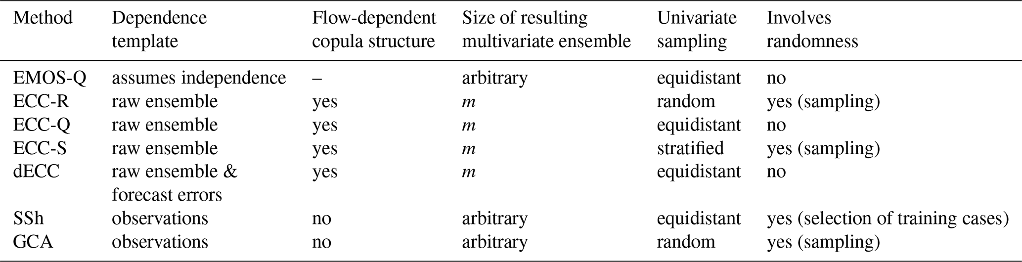
When applying univariate post-processing for each margin separately, multivariate (i.e., inter-variable, spatial, and/or temporal) dependencies across the margins are lost. These dependencies are restored in a second step. Here, we consider five different approaches to do so. An overview of selected key features is provided in Table 1. For further discussion of advantages and shortcomings, as well as comparisons of subsets of these methods, see, e.g., Schefzik et al. (2013); Wilks (2015). In the following we use z to denote univariate quantities in the individual dimensions. Z in bold print is used to represent vector-valued quantities, and Z in normal print is used for components thereof.
Table 1Overview of selected key characteristics of the multivariate post-processing methods considered in this paper.
2.2.1 Assumption of independence (EMOS-Q)
Instead of modeling the desired dependencies in any way, omitting the second step corresponds to assuming independence across the margins. To that end, a univariate sample is generated in each margin by drawing from the post-processed forecast distribution . The univariate samples are then simply combined into a corresponding vector. Following Schefzik et al. (2013), we use equidistant quantiles of at levels to generate the sample and denote this approach by EMOS-Q.
2.2.2 Ensemble copula coupling (ECC)
The basic ensemble copula coupling (ECC) approach proposed by Schefzik et al. (2013) proceeds as follows.
-
A sample , where we assume to simplify notation, of the same size m as the unprocessed ensemble is drawn from each post-processed predictive marginal distribution .
-
The sampled values are rearranged in the rank order structure of the raw ensemble; i.e., the permutation σl of the set defined by , with possible ties resolved at random, is applied to the post-processed sample from the first step in order to obtain the final ECC ensemble via
where and .
Depending on the specific sampling procedure in Step 1, we here distinguish the following different ECC variants.
-
ECC-R. The sample is randomly drawn from (and subsequently arranged in ascending order).
-
ECC-Q. The sample is constructed using equidistant quantiles of at levels :
-
ECC-S (Hu et al., 2016). First, random numbers , where for , are drawn, with 𝒰(a,b] denoting the uniform distribution on the interval (a,b]. Then, is set to the quantile of at level ui:
Besides the above sampling schemes, Schefzik et al. (2013) propose an alternative transformation approach referred to as ECC-T. This variant is in particular appealing for theoretical considerations, as it provides a link between the ECC notion and member-by-member post-processing approaches (Schefzik, 2017). However, as it may involve additional modeling steps, ECC-T is not as generic as the other schemes and thus not explicitly considered here.
2.2.3 Dual ensemble copula coupling (dECC)
Dual ECC (dECC) is an extension of ECC which aims at combining the structure of the unprocessed ensemble with a component accounting for the forecast error autocorrelation structure (Ben Bouallègue et al., 2016), proceeding as follows.
-
ECC-Q is applied in order to obtain reordered ensemble forecasts , with for .
-
A transformation based on an estimate of the error autocorrelation is applied to the bias-corrected post-processed forecast in order to obtain correction terms . Precisely, for .
-
An adjusted ensemble is derived via for .
-
ECC-Q is applied again, but now performing the reordering with respect to the rank order structure of the adjusted ensemble from Step 3 used as a modified dependence template.
2.2.4 Schaake shuffle (SSh)
The Schaake shuffle (SSh) proceeds like ECC-Q, but reorders the sampled values in the rank order structure of m past observations (Clark et al., 2004) and not with respect to the unprocessed ensemble forecasts. For a better comparison with (d)ECC, the size of SSh ensemble is restricted to equal that of the unprocessed ensemble here. However, in principle, the SSh ensemble may have an arbitrary size, provided that sufficiently many past observations are available to build the dependence template. Extensions of SSh that select past observations based on similarity are available (Schefzik, 2016; Scheuerer et al., 2017) but not explicitly considered here as their implementation is not straightforward and may involve additional modeling choices specific to the situation at hand.
The reordering-based methods considered thus far can be interpreted as non-parametric, empirical copula approaches. In particular, in the setting of Sklar's theorem, C is taken to be the empirical copula induced by the corresponding dependence template, i.e., the unprocessed ensemble forecasts in the case of ECC, the adjusted ensemble in the case of dECC, and the past observations in the case of SSh.
2.2.5 Gaussian copula approach (GCA)
By contrast, in the Gaussian copula approach (GCA) proposed by Pinson and Girard (2012) and Möller et al. (2013), the copula C is taken to be the parametric Gaussian copula. GCA can be traced back to similar ideas from earlier work in spatial statistics (e.g., Berrocal et al., 2008) and proceeds as follows.
-
A set of past observations , with , is transformed into latent standard Gaussian observations by setting
for and , where is the marginal distribution obtained by univariate post-processing. The index here refers to a training set of past observations.
-
An empirical (or parametric) (d×d) correlation matrix of the d-dimensional normal distribution in Eq. (1) is estimated from .
-
Multivariate random samples are drawn, where denotes a d-dimensional normal distribution with mean vector and estimated correlation matrix from Step 2 and for .
-
Final GCA post-processed ensemble forecast , with for , is obtained via
for and , with Φ denoting the CDF of the univariate standard normal distribution. While the size of the resulting ensemble may in principle be arbitrary, it is here set to the size m of the raw ensemble.
We consider several simulation settings to highlight different aspects and provide a broad comparison of the effects of potential misspecifications of the ensemble predictions on the performance of the various multivariate post-processing methods. The general setup of all simulation settings is as follows.
An initial training set of pairs of simulated ensemble forecasts and observations of size ninit is generated. Post-processed forecasts are then computed and evaluated over a test set of size ntest. Therefore, iterations are performed in total for all simulation settings. In the following, we set throughout.
To describe the individual settings in more detail, we here begin by first identifying the general structure of the steps that are performed in all settings. For each iteration t in both training and test sets (i.e., ), multivariate forecasts and observations are generated.
- (S1)
Generate multivariate observations and ensemble forecasts.
For all iterations t in the test set (i.e., ), the following steps are carried out.
- (S2)
Apply univariate post-processing separately in each dimension.2
- (S3)
Apply multivariate post-processing methods.
- (S4)
Compute univariate and multivariate measures of forecast performance on the test set.
Unless indicated otherwise, all simulation draws are independent across iterations. To simplify notation, we will thus typically omit the simulation iteration index t in the following.
To quantify simulation uncertainty, the above procedure is repeated 100 times for each tuning parameter combination in each setting. In the interest of brevity, we omit ECC-R, which did show substantially worse results in initial tests (see also Schefzik et al., 2013). In the following, the individual simulation settings are described in detail, and specific implementation choices are discussed.
3.1 Setting 1: multivariate Gaussian distribution
As a starting point we first consider a simulation model where observations and ensemble forecasts are drawn from multivariate Gaussian distributions.3 This setting may for example apply in the case of temperature forecasts at multiple locations considered simultaneously. The simplicity of this model allows one to readily interpret misspecifications in the mean, variance, and covariance structures.
- (S1)
For iterations , independent and identically distributed samples of observations and ensemble forecasts are generated as follows.
-
Observation: where , and for .
-
Ensemble forecasts: where , and for .
The parameters ϵ and σ introduce a bias and a misspecified variance in the marginal distributions of the ensemble forecasts. These systematic errors are kept constant across dimensions . The parameters ρ0 and ρ control the autoregressive structure of the correlation matrix of the observations and ensemble forecasts. Setting ρ0≠ρ introduces misspecifications of the correlation structure of the ensemble forecasts.
-
- (S2)
As described in Sect. 2.1, univariate post-processing is applied independently in each dimension . Here, we employ the standard Gaussian EMOS model (2) proposed by Gneiting et al. (2005). The EMOS coefficients are estimated by minimizing the mean continuous ranked probability score (CRPS; see Appendix B) over the training set consisting of the ninit initial iterations and are then used to produce out-of-sample forecasts for the ntest iterations in the test set.
- (S3)
Next, the multivariate post-processing methods described in Sect. 2.2 are applied. Implementation details for the individual methods are as follows.
-
For dECC, the estimate of the error autocorrelation is obtained from the ninit initial training iterations to compute the required correction terms for the test set.
-
To obtain the dependence template for SSh, m past observations are randomly selected from all iterations preceding the current iteration t.
-
The correlation matrix Σ required for GCA is estimated by the empirical correlation matrix based on all iterations preceding the current iteration t.
-
The verification results for all methods that require random sampling (ECC-S, SSh, GCA) are averaged over 10 independent repetitions for each iteration in the test set.
-
The multivariate Gaussian setting is implemented for d=5 and all combinations of , and . As indicated above, the simulation experiment is repeated 100 times for each of the 300 parameter combinations. If the setting from above is interpreted as a multivariate model for temperatures at multiple locations, observations from the extant literature on post-processing suggest that, typically, values of σ<1 and ρ>ρ0 would be expected in real-world datasets.
A variant of Setting 1 based on a multivariate truncated Gaussian distribution has also been investigated. Apart from a slightly worse performance of GCA, the results are similar to those of Setting 1. We thus refer to Sect. S5 of the Supplement, where details on the simulation setting and results are provided.
3.2 Setting 2: multivariate censored extreme value distribution
To investigate alternative marginal distributions employed in post-processing applications, we further consider a simulation setting based on a censored version of the generalized extreme value (GEV) distribution. The GEV distribution was introduced by Jenkinson (1955) among others, combining three different types of extreme value distributions. It has been widely used for modeling extremal climatological events such as flood peaks (e.g., Morrison and Smith, 2002) or extreme precipitation (e.g., Feng et al., 2007). In the context of post-processing, GEV distributions have for example been applied for modeling wind speed in Lerch and Thorarinsdottir (2013). Here, we consider multivariate observations and forecasts with marginal distributions given by a left-censored version of the GEV distribution which was proposed by Scheuerer (2014) in the context of post-processing ensemble forecasts of precipitation amounts.
- (S1)
For iterations samples of observations and ensemble forecasts are generated as follows. For , the marginal distributions are GEV distributions left-censored at 0,
where the distribution parameters μ (location), σ (scale), and ξ (shape) are identical across dimensions . Details on the left-censored GEV distribution are provided in Appendix A. Misspecifications of the marginal ensemble predictions are obtained by choosing different GEV parameters for observations () and forecasts (). Combined misspecifications of the three parameters result in more complex deviations of mean and variance (on the univariate level) compared to Setting 1. Typically there is a joint influence of the GEV parameters on mean and dispersion properties of the distribution. In order to exploit the complex behavior a variety of parameter combinations for observations and ensemble forecasts were considered.
To generate multivariate observations and ensemble predictions , , the so-called NORTA (normal to anything) approach is chosen; see Cario and Nelson (1997) and Chen (2001). This method allows one to generate realizations of a random vector , with specified marginal distribution functions , and a given correlation matrix . The NORTA procedure consists of three steps. In a first step a vector is generated from for a correlation matrix R∗. In a second step, u(l)=Φ(v(l)) is computed, where Φ denotes the CDF of the standard normal distribution. In a third step, is derived for , where is the inverse of . The correlation matrix R∗ is chosen in a such a way that the z(l) have the desired target correlation matrix R. Naturally, the specification of R∗ is the most involved part of this procedure. Here, we use the retrospective approximation algorithm implemented in the
RpackageNORTARA(Su, 2014). TheNORTARApackage infrequently produced error and warnings, which were not present for alternative starting values of the random number generator. Following the previous simulation settings the target correlation matrix R is chosen as for and . - (S2)
To separately post-process the univariate ensemble forecasts, we employ the EMOS method for quantitative precipitation based on the left-censored GEV distribution proposed by Scheuerer (2014). To that end we assume , such that the mean ν and the variance of the non-censored GEV distribution exist, and
where Γ denotes the gamma function and γ is the Euler–Mascheroni constant. See Appendix A for comments on mean and variance of the left-censored GEV. Following Scheuerer (2014), the parameters () are linked to the ensemble predictions via
Here, and are the arithmetic mean and the fraction of zero values of the ensemble predictions , respectively, while denotes the mean absolute difference of the ensemble predictions, i.e.,
The shape parameter ξ is not linked to the ensemble predictions, but is estimated along with the EMOS coefficients a0, a1, a2, b0, and b1. As in Scheuerer (2014), the link function refers to the parameter ν instead of μ, since it is argued that for fixed ν an increase in σ can be interpreted more naturally as an increase in uncertainty. An implementation in
Ris available in theensembleMOSpackage (Yuen et al., 2018). For our simulation, this package was not directly invoked, but the respective functions were used as a template. As described in Sect. 2.1, univariate post-processing is applied independently in each dimension . The EMOS coefficients are estimated as described above over the training set consisting of the ninit initial iterations and are then used to produce out-of-sample forecasts for the ntest iterations in the test set. - (S3)
Identical to (S3) of Setting 1, except for GCA, where we proceed differently to account for the point mass at zero. The latent standard Gaussian observations are generated by , where u is a randomly chosen value in the interval in case and in case .
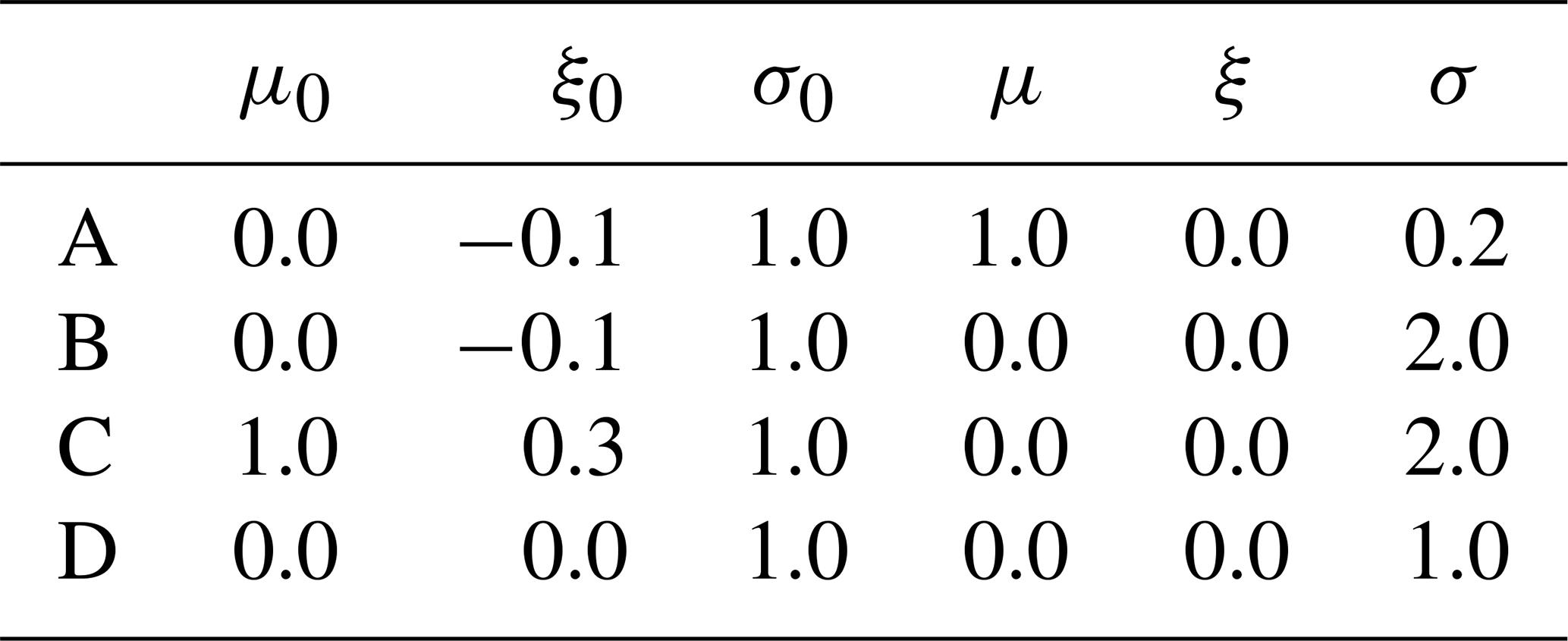
The multivariate censored extreme value setting is implemented for d=4 and four different scenarios summarized in Table 2. The choice of dimension is motivated by the fact that preliminary analyses had revealed a heavy increase in computation time and numerical problems for values of d greater than 4. In each scenario the GEV0 distribution parameters for the observations are chosen according to (), while the parameters for the ensemble predictions are chosen according to (). In both cases, the correlation matrix R from above is invoked with different choices of ρ0 and ρ from the set , giving a total of scenarios. Note that according to Scheuerer (2014) there is a positive probability for zero to occur when either ξ≤0 or ξ>0 and . The scenarios from Table 2 are chosen in such a way that either one of these two conditions is met.
The scenarios from Table 2 were not chosen to mimic real-life situations in the first place, but to emulate pronounced differences in distributions and account for a variety of misspecification types. In future research a more detailed and data-based study of the properties of the GEV0 in ensemble post-processing of precipitation is planned, which might give further insight into the correspondence (and interplay) of the GEV0 parameters to typically occurring situations for precipitation.
3.3 Setting 3: multivariate Gaussian distribution with changes over time
In the preceding simulation settings, the misspecifications of the ensemble forecasts were kept constant over the iterations within the simulation experiments. However, forecast errors of real-world ensemble predictions often exhibit systematic changes over time, for example due to seasonal effects or differences in flow-dependent predictability due to variations of large-scale atmospheric conditions. Here, we modify the multivariate Gaussian simulation setting from Sect. 3.1 to introduce changes in the mean, variance, and covariance structure of the multivariate distributions of observations and ensemble forecasts. In analogy to practical applications of multivariate post-processing, the ensemble predictions and observations may be interpreted as multivariate in terms of location or prediction horizon, with changes in the misspecification properties over time.
- (S1)
For iterations , independent samples of observations and ensemble forecasts are generated as follows.
-
Observation: where . To obtain the correlation matrix Σ0, let for and The covariance matrix S0 is scaled into the corresponding correlation matrix Σ0 using the
Rfunctioncov2cor(). -
Ensemble forecasts: where . To obtain the correlation matrix Σ we proceed as for the observations; however, we set for (i.e., ρ0 is replaced by ρ).
In contrast to Setting 1, the misspecifications in the mean and correlation structure now include a periodic component. The above setup will be denoted by Setting 3A.
Following a suggestion from an anonymous reviewer, we further consider a variant which we refer to as Setting 3B. For iterations we generate independent samples of observations and ensemble forecasts as follows.
-
Observation: where . To obtain a correlation matrix Σ(t) that varies over iterations, we set for , where the correlation parameter ρ0(t) varies over iterations according to
for . The lag-1 correlations thus oscillate between ρ0 and .
-
Ensemble forecasts: where . Similarly to the observations, we set for , where
with a from above. The correlations for the ensemble member forecasts thus oscillate between ρ and .
Settings 3A and 3B differ in the variations of the mean and covariance structure over time. For both, we proceed as follows.
-
- (S2)
As in Setting 1, we employ the standard Gaussian EMOS model (2). However, to account for the changes over iterations we now utilize a rolling window consisting of pairs of ensemble forecasts and observations from the 100 iterations preceding t as a training set to obtain estimates of the EMOS coefficients. See Lang et al. (2020) for a detailed discussion of alternative approaches to incorporate time dependence in the estimation of post-processing models.
- (S3)
The application of the multivariate post-processing methods is identical to the approach taken in Setting 1. Note that we deliberately follow the naive standard implementations (see Sect. 2.2) here to highlight some potential issues of the Schaake shuffle in this context.
Setting 3A is implemented for and all combinations of . For Setting 3B, we investigate separate sets of low (ρ0=0.25), medium (ρ0=0.5), and high (ρ0=0.75) true correlation, with corresponding choices of ρ with low (), medium (), and high () values, respectively. Further, values of , and are considered for each of these sets. As before simulation experiments are repeated 100 times for each of the parameter combinations.
In the following, we focus on comparisons of the relative predictive performance of the different multivariate post-processing methods and apply proper scoring rules for forecast evaluation. In particular, we use the energy score (ES; Gneiting et al., 2008) and variogram score of order 1 (VS; Scheuerer and Hamill, 2015) to evaluate multivariate forecast performance. Diebold–Mariano (DM; Diebold and Mariano, 1995) tests are applied to assess the statistical significance of the score differences between models. Details on forecast evaluation based on proper scoring rules and DM tests are provided in Appendix B. Note that proper scoring rules are often used in the form of skill scores to investigate relative improvements in predictive performance in the meteorological literature. Here, we instead follow suggestions of Ziel and Berk (2019), who argue that the use of DM tests is of crucial importance to appropriately discriminate between multivariate models.
While our focus here is on multivariate performance, we briefly demonstrate that the univariate post-processing models applied in the different simulation settings usually work as intended.

Figure 1Summaries of DM test statistic values based on the CRPS. ECC-Q forecasts are used as a reference model such that positive values of the test statistic indicate improvements over ECC-Q and negative values indicate deterioration of forecast skill. Boxplots summarize results from multiple parameter combinations for the simulation settings, with potential restrictions on the simulation parameters indicated in the plot title. For example, boxplots in the first panel summarize simulation results from all parameter combinations of Setting 1 (and the 100 Monte Carlo repetitions each) subject to ϵ=1. The horizontal gray stripe indicates the acceptance region of the two-sided DM test under the null hypothesis of equal predictive performance at a level of 0.05.
4.1 Univariate performance
The univariate predictive performance of the raw ensemble forecasts in terms of the CRPS is improved by the application of univariate post-processing methods across all parameter choices in all simulation settings. The magnitude of the relative improvements by post-processing depends on the chosen simulation parameters: exemplary results are shown in Fig. 1. The results for Setting 2 are omitted as they vary more and strongly depend on the simulation parameters.
ECC-Q does not change the marginal distributions; the univariate forecasts are thus identical to solely applying univariate post-processing methods in the margins separately, without accounting for dependencies. We will later refer to this as EMOS-Q. Note that for ECC-S and SSh differences in the univariate forecast distributions compared to those of ECC-Q may arise from randomly sampling the quantile levels in ECC-S and from random fluctuations due to the 10 random repetitions that were performed to account for the simulation uncertainty of those methods. However, we found the effects on the univariate results to be negligible and omit ECC-S, dECC, and SSh from Fig. 1.
For the simulation parameter values summarized there, univariate post-processing works as intended with statistically significant improvements over the raw ensemble forecasts. Note that for GCA the univariate marginal distributions are modified due to the transformation step in Eq. (4). While the quantile forecasts of ECC-Q are close to optimal in terms of the CRPS (Bröcker, 2012), (randomly sampled) univariate GCA forecasts do not possess this property, resulting in worse univariate performance compared to all other methods.
4.2 Multivariate performance
We now compare the multivariate performance of the different post-processing approaches presented in Sect. 2.2. Multivariate forecasts obtained by only applying the univariate post-processing methods without accounting for dependencies (denoted by EMOS-Q) as well as the raw ensemble predictions (ENS) are usually significantly worse and will be omitted in most comparisons below unless indicated otherwise. Additional figures with results for all parameter combinations in all settings are provided in the Supplement.
4.2.1 Setting 1: multivariate Gaussian distribution
The tuning parameter ϵ governing the bias in the mean vector of the ensemble forecasts only has very limited effects on the relative performance of the multivariate post-processing methods. To retain focus we restrict our attention to ϵ=1. Figure 2 shows results in terms of the ES for two different choices of σ, using multivariate forecasts of ECC-Q as the reference method. For visual clarity, we omit parameter combinations where either or . Corresponding results are available in the Supplement. Note that the relative forecast performance of all approaches except for dECC generally does not depend on σ. We thus proceed to discuss the remaining approaches first and dECC last.
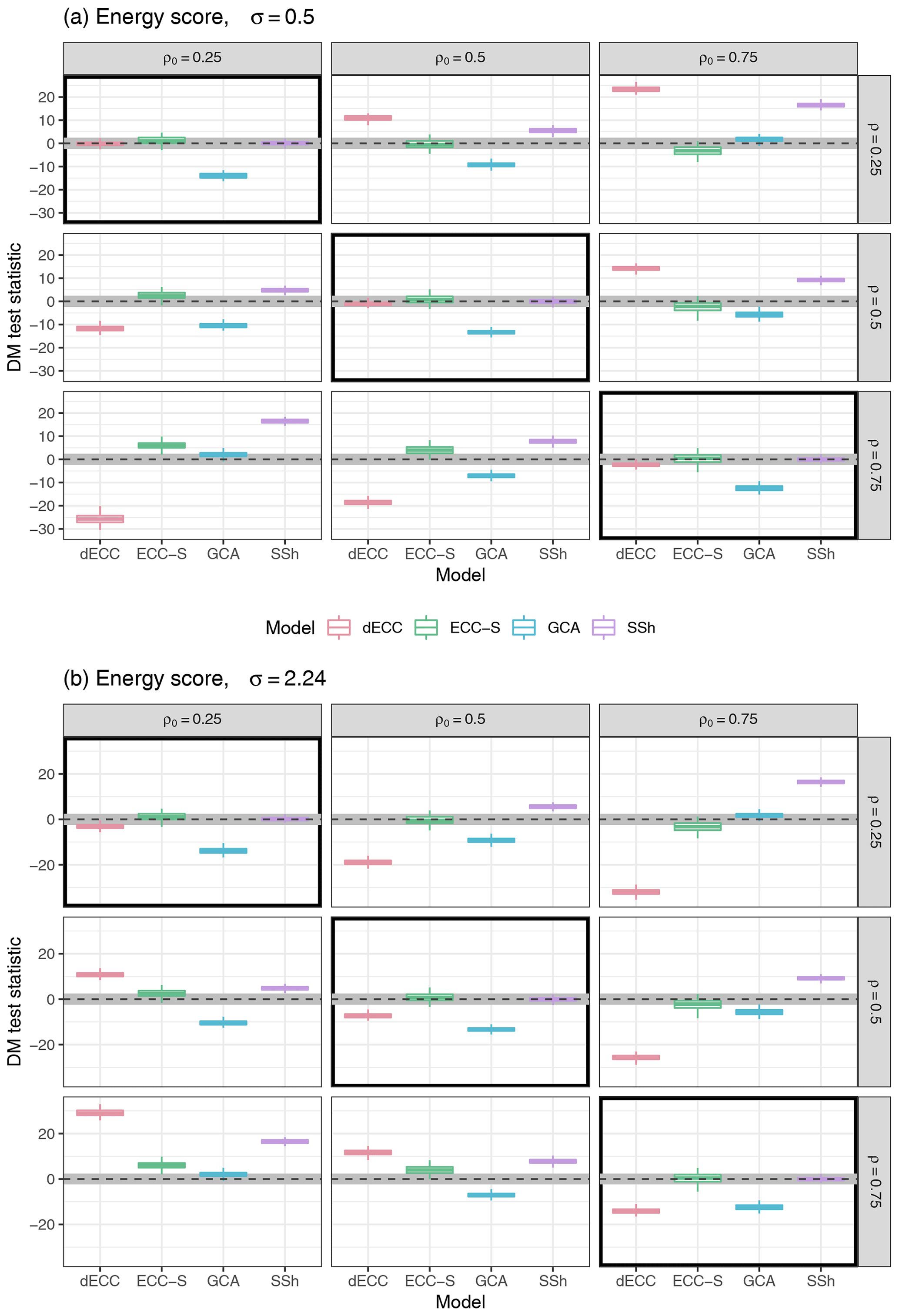
Figure 2Summaries of DM test statistic values based on the ES for Setting 1 with ϵ=1, and σ=0.5 (a) and (b). ECC-Q forecasts are used as a reference model such that positive values of the test statistic indicate improvements over ECC-Q and negative values indicate deterioration of forecast skill. Boxplots summarize results of the 100 Monte Carlo repetitions of each individual experiment. The horizontal gray stripe indicates the acceptance region of the two-sided DM test under the null hypothesis of equal predictive performance at a level of 0.05. Simulation parameter choices where the correlation structure of the raw ensemble is correctly specified (ρ=ρ0) are surrounded by black boxes.
If the correlation structure of the unprocessed ensemble forecasts is correctly specified (i.e., ρ=ρ0), no significant differences can be detected between ECC-Q, ECC-S, and SSh. In contrast, GCA (and dECC for larger values of σ) performs substantially worse. The worse performance of GCA might be due to the larger forecast errors in the univariate margins; see Sect. 4.1.
In the cases with misspecifications in the correlation structure (i.e., ρ≠ρ0), larger differences can be detected among all the methods. Notably, SSh never performs substantially worse than ECC-Q and is always among the best performing approaches. This is not surprising as the only drawback of SSh in the present context and under the chosen implementation details is the underlying assumption of time invariance of the correlation structure, which will be revisited in Setting 3. The larger the absolute difference between ρ and ρ0, the greater the improvement of SSh relative to ECC-Q. This is due to the fact that it becomes more and more beneficial to learn the dependence template from past observations rather than the raw ensemble, the less information the ensemble provides about the true dependence structure. GCA also tends to outperform ECC-Q if the differences between ρ and ρ0 are large; however, GCA always performs worse than SSh and shows significantly worse performance than ECC-Q if the misspecifications in the ensemble are not too large (i.e., if ρ and ρ0 are equal or similar).
The relative performance of ECC-S depends on the ordering of ρ and ρ0. If ρ>ρ0, ECC-S significantly outperforms ECC-Q; however, if ρ<ρ0 significant ES differences in favor of ECC-Q can be detected. For dECC, the performance further depends on the misspecification of the variance structure in the marginal distributions. If ρ>ρ0, the DM test statistic values move from positive (improvement over ECC-Q) to negative (deterioration compared to ECC-Q) values for increasing σ. By contrast, if ρ<ρ0 the values of the test statistic instead change from negative to positive for increasing σ. The differences are mostly statistically significant and indicate the largest relative improvements among all methods in cases of the largest possible differences between ρ and ρ0. However, note that for some of those parameter combinations with small ρ and large ρ0, even EMOS-Q can outperform ECC-Q and ECC-S. In these situations, the raw ensemble forecasts contain very little information about the dependence structure, and the ES can be improved by assuming independence instead of learning the dependence template from the ensemble.
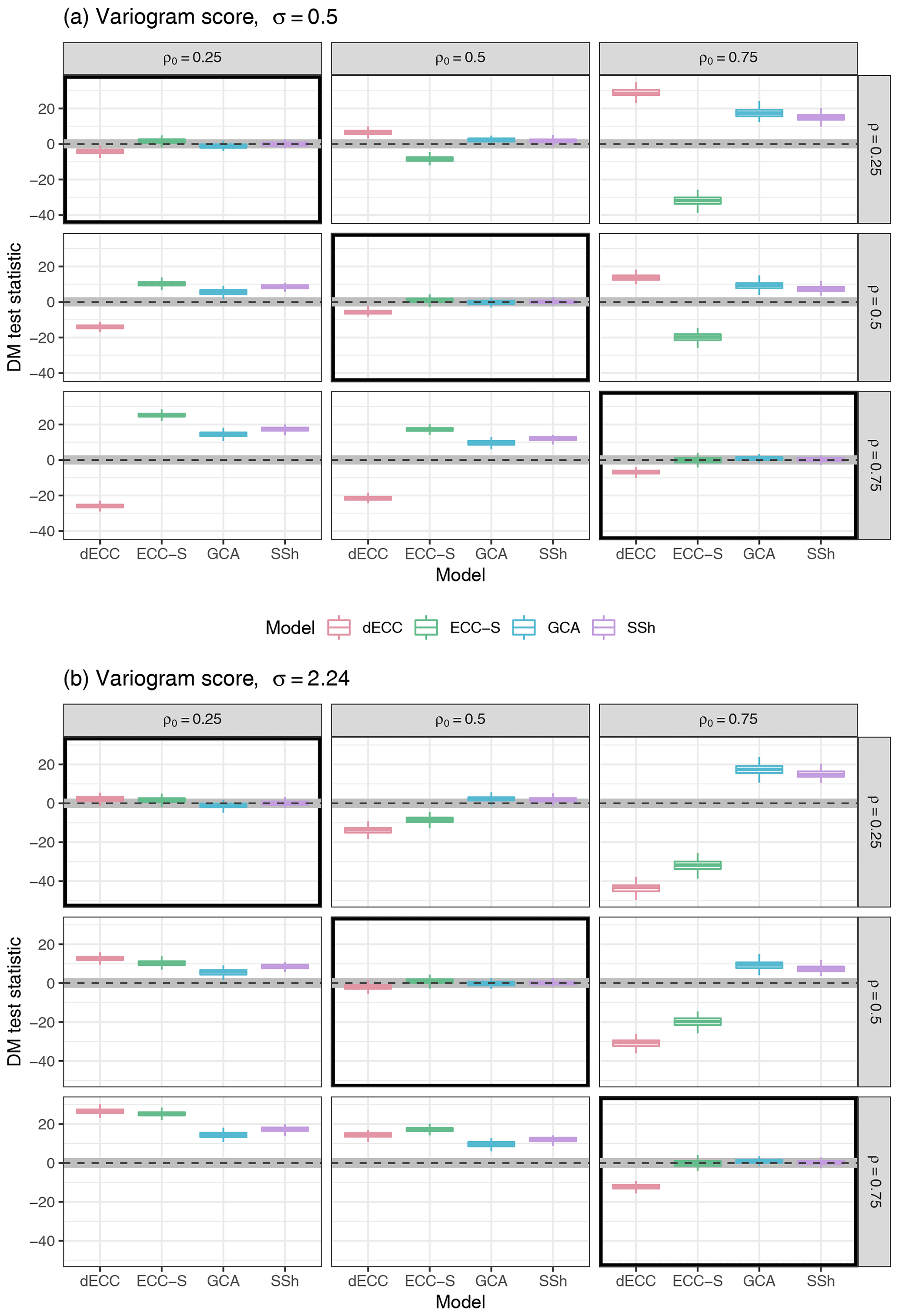
Results in terms of the VS are shown in Fig. 3. Most of the conclusions from the results in terms of the ES extend directly to comparisons based on the VS. SSh consistently remains among the best performing methods and provides significant improvements over ECC-Q unless ρ=ρ0; however, alternative approaches here outperform SSh more often. Notably, the relative performance of GCA is consistently better in terms of the VS than in terms of the ES. For example, the differences between GCA and SSh appear to generally be negligible, and GCA does not perform worse than ECC-Q for any of the simulation parameter combinations. These differences between the results for GCA in terms of ES and VS may be explained by the greater sensitivity of the VS to misspecifications in the correlation structure, whereas the ES shows a stronger dependence on the mean vector.
For ECC-S and dECC, the general dependence on values of ρ, ρ0, and σ (for dECC) is similar to the results for the ES, but the magnitude of both positive as well as negative differences to all other methods is increased. For example, it is now possible to find parameter combinations where either ECC-S or dECC (or both) substantially outperform both GCA and SSh.
The role of ensemble size m
To assess the effect of the ensemble size m on the results, additional simulations have been performed with the simulation parameters from Fig. 2 but with ensemble sizes between 5 and 100. Corresponding figures are provided in the Supplement. Overall, the relative ranking of the different methods is only very rarely affected by changes in the ensemble size. The relative differences in terms of the ES between ECC-Q and ECC-S and between ECC-Q and GCA become increasingly negligible with increasing ensemble size. Further, SSh shows improved predictive performance for larger numbers of ensemble members for ρ0<ρ in the case of the ES and for ρ0>ρ in the case of the VS. The relative performance of dECC is strongly affected by changes in m for large misspecifications in the correlation parameters. A positive effect of larger numbers of members relative to ECC-Q in terms of both scoring rules can be detected for ρ0>ρ when σ<1 and for ρ0<ρ when σ>1. In both cases, the corresponding effects are negative if the misspecification in σ is reversed.
The role of dimension d
Additional simulations were further performed with dimensions d between 2 and 50 and the simulation parameters from above. In the interest of brevity, we refer to the Supplement for corresponding figures. In terms of the ES, the results for ECC-S are largely not affected by changes in dimension, whereas the relative performance of ECC-S improves with increasing d, and minor improvements over ECC-Q can be detected even for correctly specified correlation parameters for high dimensions. For GCA, a marked deterioration of relative skill can be observed in terms of the ES, which can likely be attributed to the sampling effects discussed above. In terms of the VS, GCA partly shows the best relative performance among all methods for dimensions between 10 and 20 and performs worse in higher dimensions. The relative differences in predictive performance in favor of SSh are more pronounced in larger dimensions, in particular in cases with large misspecification of the correlation parameters. Changes in the relative performance of dECC in terms of both scoring rules for increasing numbers of dimensions are similar to those observed for increasing numbers of ensemble members.
4.2.2 Setting 2: multivariate censored GEV distributions
The four considered scenarios in Table 2 constitute different types of deviation of the ensemble from the observation properties. Results for Scenario B are given below in Fig. 4, while the corresponding figures for Scenarios A, C, and D can be found in Sect. S2.1. As the GEV0 distribution yields extreme outliers much more frequently than the Gaussian distribution in Setting 1, all figures (here and in the Supplement) show only those values that are within the 1.5× interquartile range, so that the overall comparison of the boxplots does not suffer from single extreme outliers.
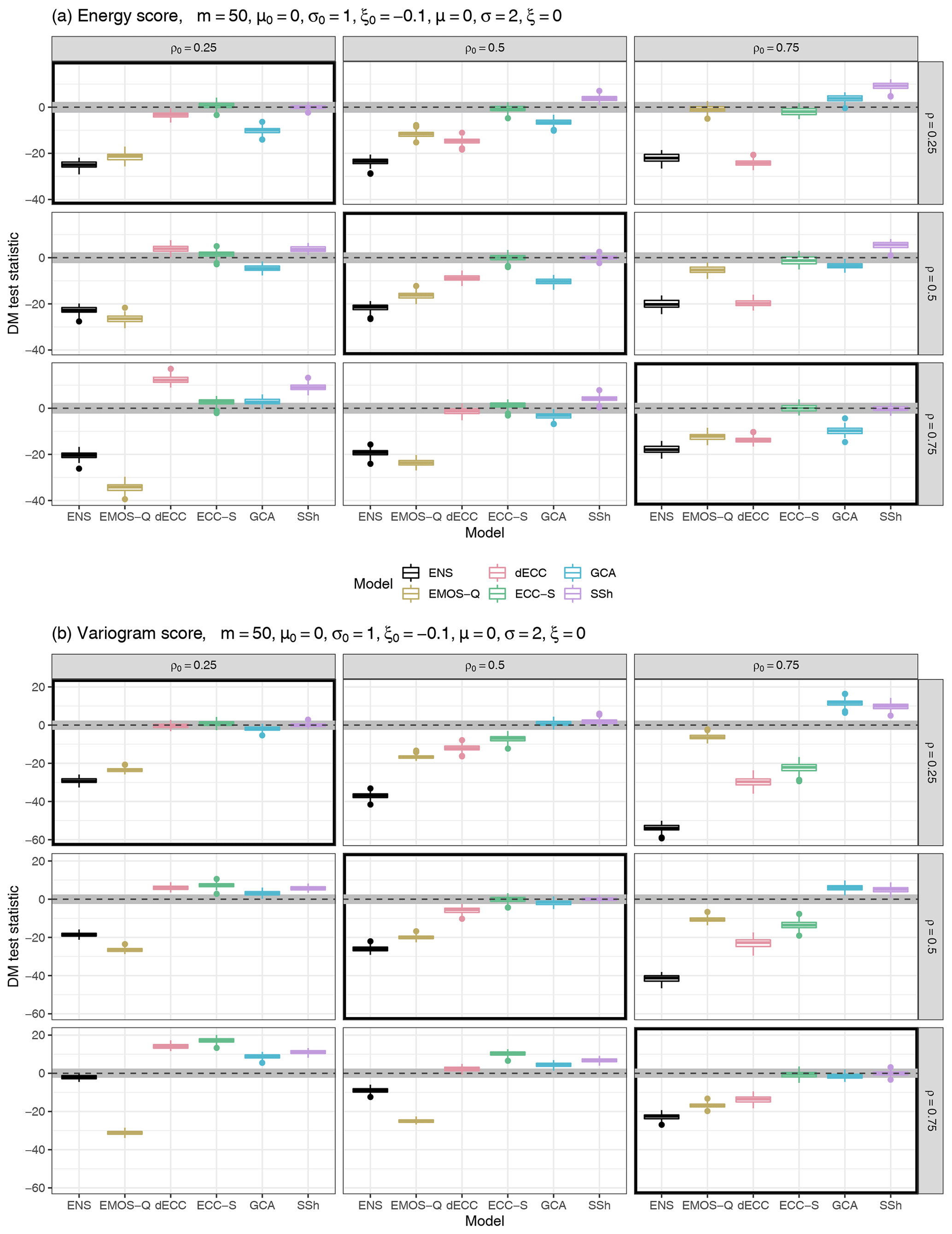
Figure 4Summaries of DM test statistic values based on the ES (a) and the VS (b) for Setting 2, Scenario B from Table 2, based on m=50 ensemble members. ECC-Q forecasts are used as a reference model such that positive values of the test statistic indicate improvements over ECC-Q and negative values indicate deterioration of forecast skill. Boxplots summarize results of the 100 Monte Carlo repetitions of each individual experiment. The horizontal gray stripe indicates the acceptance region of the two-sided DM test under the null hypothesis of equal predictive performance at a level of 0.05.
-
In Scenario B the location is correctly specified, but scale and shape are misspecified such that ensemble forecasts have both larger scale and shape, resulting in a heavier right tail and slightly higher point masses at zero. This scenario is taken as a reference among the four considered ones and shown in Fig. 4. Additional figures with results for the remaining scenarios are provided in the Supplement. Multivariate post-processing improves considerably upon the raw ensemble. ECC-Q is outperformed by SSh and GCA only when the absolute difference between ρ0 and ρ becomes larger. As before, this is likely caused by the use of past observations to determine the dependence template by GCA and SSh, which proves beneficial in comparison to ECC-Q in cases of a highly incorrect correlation structure in the ensemble. For correctly specified correlations (panels on the main diagonal in Fig. 4), the relative performance of the methods does not depend on the actual value of correlation.
-
In Scenario A the observation location parameter is shifted from 0 to a positive value for the ensemble, the observation scale is larger, and the shape is smaller than in the ensemble. Therefore, the ensemble forecasts come from a distribution with smaller spread than the observations, which is also centered away from 0 and has lower point mass at 0. In comparison to Scenario B there are more outliers, especially for ECC-S. In the case of correctly specified correlations, the performance of the methods also does not depend on the actual value of correlation as in Scenario B. Notably, EMOS-Q here performs mostly similar to the ensemble, while in the other three scenarios it typically performs worse than the ensemble if ρ>ρ0.
-
In Scenario C the observation location is larger, the scale smaller, and the shape larger than in the ensemble distribution. This results in an observation distribution with a much heavier right tail and a much larger point mass at 0 compared to the ensemble distribution. Here, post-processing models frequently offer no or only slight improvements over the raw ensemble. While ECC-Q does not always outperform the raw ensemble forecasts, SSh still shows improved forecast performance. As in the other scenarios, in the case of correctly specified correlations, the performance of the methods does not depend on the actual value of correlation.
-
In Scenario D all univariate distribution parameters are correctly specified. Therefore, the main differences in performance are imposed by the different misspecifications of the correlation structure. The main difference compared to the other scenarios is given by the markedly worse effects of not accounting for multivariate dependencies during post-processing (EMOS-Q).
In general, the methods perform differently across the four scenarios, but for most situations multivariate post-processing improves upon univariate post-processing without accounting for dependencies. Furthermore, SSh reveals a good performance in all four scenarios when ρ0 differs considerably from ρ. The performance of SSh has a tendency to improve further when the observation correlation is larger than the ensemble correlation. Within each of the four scenarios, the performance of the methods is nearly identical in cases where the correlation is correctly specified. In other words, as long as the ensemble forecasts correctly represent the correlation of the observations, the actual value of the correlation does not have an impact on the performance of a multivariate post-processing method. Above-described observations can be found in terms of both the ES and the VS.
In addition to the scenarios from Table 2, further scenario variations were considered for ρ0=0.75 and ρ=0.25, that is, for the case where ensemble correlation is too low compared to the observations. Figure 5 shows the situation where the observation location parameter is larger, the scale smaller, but the shape also smaller than in the ensemble forecasts. This contrasts with the situation in Scenario C. While in C the observations were heavier tailed with higher point mass at 0, here it is the other way round (the ensemble distribution is heavier tailed with higher point mass at 0). In accordance with Scenarios A, B, and C (where there are parameter misspecifications in the ensemble compared to the observations), EMOS-Q performs better than the raw ensemble and also better than dECC (as in B and C), while SSh and GCA perform best. However, in contrast to results in terms of the ES, GCA exhibits an even better performance compared to the other models in terms of the VS. This indicates that the VS is better able to account for the correctly specified (or by post-processing improved) correlation structure than the ES.

The role of ensemble size m
To assess the effect of the ensemble size m, additional simulations have been performed for each of the four scenarios in Table 2 with ensemble sizes between 5 and 100. Corresponding comparative figures comparing ensemble sizes m=5, 20, 50, and 100 for Scenarios A, B, C, and D are provided in Sect. S2.2. Overall, the size of the ensemble only has a minor effect on the relative performance of the multivariate methods apart from GCA, which strongly benefits from an increasing number of members across all four scenarios, specifically with regard to ES. This improvement is likely due to the sampling issues discussed above and is less pronounced in terms of the VS. As in Setting 1 the relative differences between ECC-Q and ECC-S in terms of the ES become increasingly negligible with increasing ensemble size in all considered scenarios (especially for ρ0=ρ). This phenomenon is also less pronounced for the VS. In contrast to the methods using the dependence information, the performance of EMOS-Q (not accounting for dependence) compared to ECC-Q becomes increasingly worse for an increasing number of members when measured by ES. For VS, the influence of the number of members on EMOS-Q is only small. Interestingly, the difference in performance of the raw ensemble for an increasing number of members is negligible in case the misspecification is only minor and ES is considered. In case there is no misspecification (Scenario D), the raw ensemble can slightly benefit from an increasing number of members. Similarly to the effect for ECC-Q, when measuring performance with VS, the effect on the raw ensemble is negligible. Further, it can be observed that the difference of the results between varying numbers of members is smallest for ρ0=ρ.
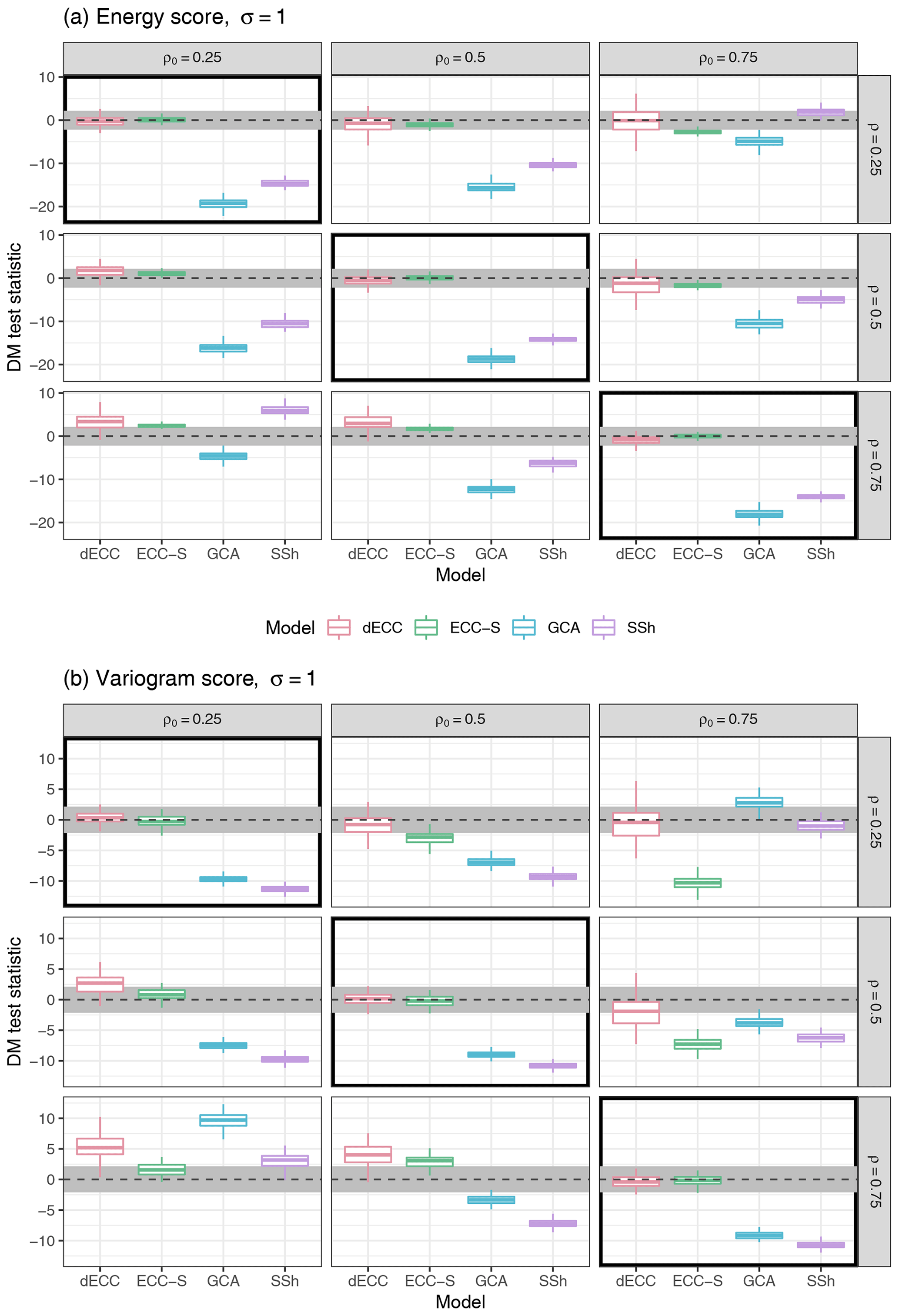
Figure 6Summaries of DM test statistic values based on the ES (a) and the VS (b) for Setting 3A with ϵ=1 and σ=1. ECC-Q forecasts are used as a reference model such that positive values of the test statistic indicate improvements over ECC-Q and negative values indicate deterioration of forecast skill. Boxplots summarize results of the 100 Monte Carlo repetitions of each individual experiment. The horizontal gray stripe indicates the acceptance region of the two-sided DM test under the null hypothesis of equal predictive performance at a level of 0.05. Simulation parameter choices where the correlation structure of the raw ensemble is correctly specified (ρ=ρ0) are surrounded by black boxes.
4.2.3 Setting 3: multivariate Gaussian distribution with changes over iterations
Figure 6 shows results in terms of ES and VS for Setting 3A. We again only show results for and refer to the Supplement for further results. The most notable differences compared to Setting 1 are that the different ECC variants here significantly outperform GCA and SSh not only for ensemble forecasts with correctly specified correlation structure, but also for small deviations of ρ from ρ0. Significant ES differences in favor of SSh are only obtained for large absolute differences of ρ and ρ0. Similar observations hold for GCA which, however, generally exhibits worse performance compared to SSh. The ES differences among the ECC variants are only minor and usually not statistically significant.
Similar conclusions apply for the VS; however, GCA generally performs better than SSh, and ECC-S provides significantly worse forecasts compared to the other ECC variants for ρ<ρ0.
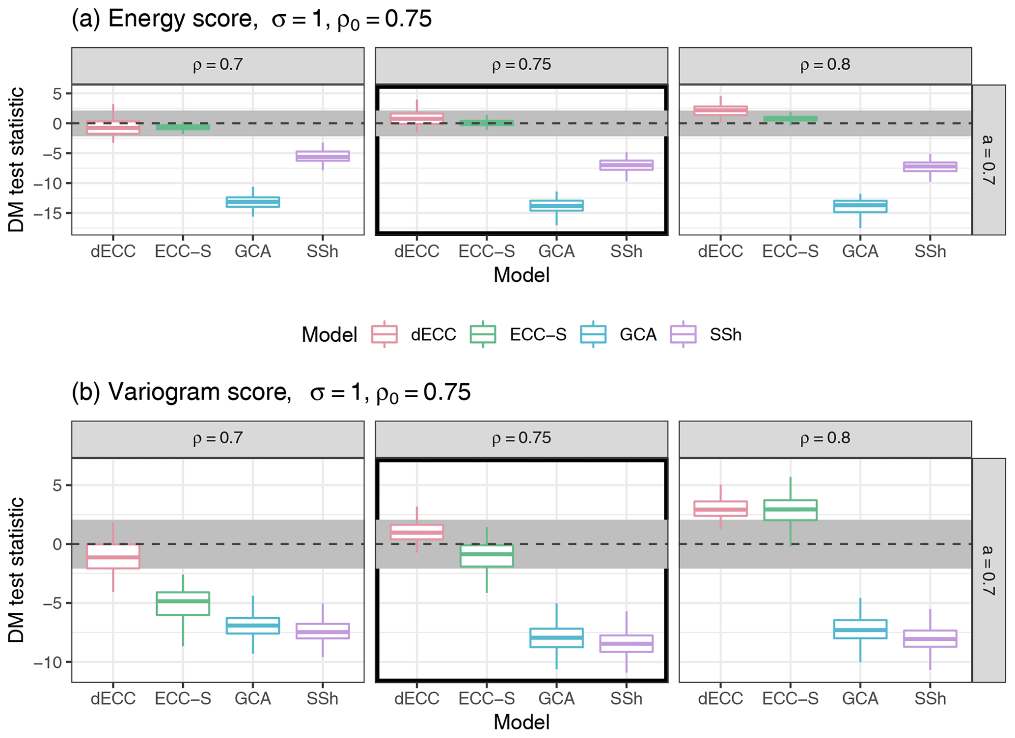
Figure 7Summaries of DM test statistic values based on the ES (a) and the VS (b) for Setting 3B for σ=1 and high values of ρ,ρ0. ECC-Q forecasts are used as a reference model such that positive values of the test statistic indicate improvements over ECC-Q and negative values indicate deterioration of forecast skill. Boxplots summarize results of the 100 Monte Carlo repetitions of each individual experiment. The horizontal gray stripe indicates the acceptance region of the two-sided DM test under the null hypothesis of equal predictive performance at a level of 0.05. Simulation parameter choices where the correlation structure of the raw ensemble is correctly specified (ρ=ρ0) are surrounded by black boxes.
Results for Setting 3B are shown in Fig. 7. Note that the columns here show different values of ρ and the row refers to a specific value of a. Similar to Setting 3A, we observe that in terms of the ES, dECC and ECC-S do not show significant differences in performance compared to ECC-Q, whereas GCA and SSh here perform worse for all parameter combinations. In terms of the VS, GCA now also performs worse than ECC-Q for all correlation parameters, whereas significantly negative and positive differences of ECC-S and dECC compared to ECC-Q can be detected for ρ<ρ0 and ρ>ρ0, respectively. Additional results for varying values of σ and a and sets of low or medium correlations are provided in the Supplement. The results generally do not depend on the choice of σ. Results for low and medium correlation parameter values are characterized by less substantial differences between the methods. In particular, it is only rarely possible to detect significant differences when comparing ECC-Q and SSh, and GCA only performs significantly worse in terms of the ES. Further, there exist more parameter combinations with improvements by ECC-S and dECC. However, note that due to the setup of Setting 3B, the variations over time in both observations and ensemble predictions will be much smaller than for high correlation parameter values. Within a fixed set of correlation parameters, the relative differences between the methods become more pronounced with increasing values of a.
Note that the main focus in both variants of Setting 3 was to demonstrate that in (potentially more realistic) settings with changes over time, naive implementations of the Schaake shuffle can perform worse than ECC variants. However, similarity-based implementations of the Schaake shuffle (Schefzik, 2016; Scheuerer et al., 2017) are available and may be able to alleviate this issue.
State-of-the-art methods for multivariate ensemble post-processing were compared in simulation settings which aimed to mimic different situations and challenges occurring in practical applications. Across all settings, the Schaake shuffle constitutes a powerful benchmark method that proves difficult to outperform, except for naive implementations in the presence of structural change (for example, time-varying correlation structures considered in Setting 3). By contrast to SSh, the Gaussian copula approach typically only provides improvements over variants of ensemble copula coupling if the parametric assumption of a Gaussian copula is satisfied or if forecast performance is evaluated with the variogram score. Results in terms of the CRPS further highlight an additional potential disadvantage in that the univariate forecast errors are larger compared to the competitors.
Not surprisingly, variants of ensemble copula coupling typically perform the better the more informative the ensemble forecasts are about the true multivariate dependence structure. A particular advantage compared to standard implementations of SSh and GCA illustrated in Setting 3 may be given by the ability to account for flow-dependent differences in the multivariate dependence structure if those are (at least approximately) present in the ensemble predictions, but not in a randomly selected subset of past observations.
There is no consistently best method across all simulation settings and potential misspecifications among the different ECC variants investigated here (ECC-Q, ECC-S, and dECC). ECC-Q provides a reasonable benchmark model and will rarely yield the worst forecasts among all ECC variants. Significant improvements over ECC-Q may be obtained by ECC-S and dECC in specific situations, including specific combinations of ensemble size and dimension. For example, dECC sometimes works well for underdispersive ensembles where the correlation is too low, whereas ECC-S may work better if the ensemble is underdispersive and the correlation is too strong. However, the results will strongly depend on the exact misspecification of the variance–covariance structure of the ensemble as well as the performance measure chosen for multivariate evaluation.
In light of the presented results it seems to be generally advisable to first test the Schaake shuffle along with ECC-Q. If structural assumptions about specific misspecifications of the ensemble predictions seem appropriate, extensions by other variants of ECC or GCA might provide improvements. However, it should be noted that the results for real-world ensemble prediction systems may be influenced by many additional factors and may differ when considering station-based or grid-based post-processing methods. The computational costs of all presented methods are not only negligible in comparison to the generation of the raw ensemble forecasts, but also compared to the univariate post-processing as no numerical optimization is required. It may thus be generally advisable to compare multiple multivariate post-processing methods for the specific dataset and application at hand.
The simulation settings considered here provide several avenues for further generalization and analysis. For example, a comparison of forecast quality in terms of multivariate calibration (Thorarinsdottir et al., 2016; Wilks, 2017) is left for future work. Further, the autoregressive structure of the correlations across dimensions may be extended towards more complex correlation functions; see, e.g., Thorarinsdottir et al. (2016, Sect. 4.2). While we only considered multivariate methods based on a two-step procedure combining univariate post-processing and dependence modeling via copulas, an extension of the comparison to parametric approaches along the lines of Feldmann et al. (2015) and Baran and Möller (2015) presents another starting point for future work. Note that within the specific choices for Setting 1, the spatial EMOS approach of Feldmann et al. (2015) can be seen as a special case of GCA.
We have limited our investigation to simulation studies only as those settings allow one to readily assess the effects of different types of misspecifications of the various multivariate properties of ensemble forecasts and observations and may thus help to guide implementations of multivariate post-processing. Further, they are able to provide a more complete picture of the effects of different types of misspecifications on the performance of the different methods than those that may be observed in practical applications. Nonetheless, an important aspect for future work is to complement the comparison of multivariate post-processing methods by studies based on real-world datasets of ensemble forecasts and observations, extending existing comparisons of subsets of the methods considered here (e.g., Schefzik et al., 2013; Wilks, 2015). However, the variety of application scenarios, methods, and implementation choices likely requires large-scale efforts, ideally based on standardized benchmark datasets. A possible intermediate step might be given by the use of simulated datasets obtained via stochastic weather generators (see, e.g., Wilks and Wilby, 1999) which may provide arbitrarily large datasets with possibly more realistic properties than the simple settings considered here.
A different perspective on the results presented here concerns the evaluation of multivariate probabilistic forecasts. In recent work Ziel and Berk (2019) argue that the use of Diebold–Mariano tests is of crucial importance for appropriately assessing the discrimination ability of multivariate proper scoring rules and find that the ES might not have as bad a discrimination ability as indicated by earlier research. The simulation settings and comparisons of multivariate post-processing methods considered here may be seen as additional simulation studies for assessing the discrimination ability of multivariate proper scoring rules. In particular, the results in Sect. 4 are in line with the findings of Ziel and Berk (2019) in that the ES does not exhibit inferior discrimination ability compared to the VS. Nonetheless, the ranking of the different multivariate post-processing methods strongly depends on the proper scoring rule used for evaluation, and further research on multivariate verification is required to address open questions, improve mathematical understanding, and guide model comparisons in applied work.
When the GEV distribution is left-censored at zero, its cumulative distribution function can be written as
for y∈𝔜, where when ξ>0, when ξ=0, and when ξ<0. This describes a three-parameter distribution family, where μ∈ℝ, σ>0, and ξ∈ℝ are location, scale, and shape of the non-censored GEV distribution, respectively.
A1 Expectation and variance
Let Y be a random variable distributed according to GEV and censored at zero to the left. From the law of total expectation,
where the second term in the sum is given by
Here, 𝕀 denotes the indicator function, g is any function of Y such that g(Y) is a random variable, and fY is the probability density function (PDF) of the non-censored GEV. By noting that , expectation and variance of the left-censored GEV can be computed from the two integrals and , the former existing when ξ<1 and the latter existing when ξ<0.5. Both integrals are not derived analytically here, but evaluated by numerical integration. In contrast to the non-censored GEV distribution, the variance of the left-censored version also depends on the parameter μ, since different choices of μ lead to different left-censored CDFs which are not merely distinguished by location. Therefore μ is a location parameter for the non-censored GEV, but not for the left-censored version.
B1 Proper scoring rules
The comparative evaluation of probabilistic forecasts is usually based on proper scoring rules. A proper scoring rule is a function
which assigns a numerical score S(F,y) to a pair of a forecast distribution F∈ℱ and a realizing observation y∈Ω. Here, ℱ denotes a class of probability distributions supported on Ω. The forecast distribution F may come in the form of a predictive CDF, a PDF, or a discrete sample as in the case of ensemble predictions. A scoring rule is called proper if
for all and strictly proper if equality holds only if F=G. See Gneiting and Raftery (2007) for a review of proper scoring rules from a statistical perspective.
The most popular example of a univariate (i.e., Ω⊂ℱ) proper scoring rule in the environmental sciences is given by the continuous ranked probability score (CRPS),
Over the past years a growing interest in multivariate proper scoring rules has accompanied the proliferation of multivariate probabilistic forecasting methods in applications across disciplines. The definition of proper scoring rules from above straightforwardly extends towards multivariate settings (i.e., Ω⊂ℱd). A variety of multivariate proper scoring rules has been proposed over the past years, usually focused on cases where multivariate probabilistic forecasts are given as samples from the forecast distributions.
To introduce multivariate scoring rules, let and let F denote a forecast distribution on ℱd given by m discrete samples from F with . Important examples of multivariate proper scoring rules include the energy score (ES; Gneiting et al., 2008),
where is the Euclidean norm on ℝd, and the variogram score of order p (VSp; Scheuerer and Hamill, 2015),
Here, wi,j is a non-negative weight that allows one to emphasize or down-weight pairs of component combinations, and p is the order of the variogram score. Following suggestions of Scheuerer and Hamill (2015), we considered p=0.5 and p=1. As none of the simulation settings indicated any substantial differences, we set p=1 throughout and denote VS1(F,y) by VS(F,y). Since the generic multivariate structure of the simulation settings does not impose any meaningful structure in pairs of components, we focus on the unweighted versions of the variogram score. Several weighting schemes have been tested but did not lead to any substantially different conclusions.
We utilize implementations provided in the R package scoringRules (Jordan et al., 2019) to compute univariate and multivariate scoring rules for forecast evaluation and post-processing model estimation.
B2 Diebold–Mariano tests
Statistical tests of equal predictive performance are frequently used to assess the statistical significance of observed score differences between models. We focus on Diebold–Mariano (DM; Diebold and Mariano, 1995) tests which are widely used in the econometric literature due to their ability to account for temporal dependencies. For applications in the context of post-processing, see, e.g., Baran and Lerch (2016).
For a (univariate or multivariate) proper scoring rule S and sets of two competing probabilistic forecasts Fi and Gi, over a test set, the test statistic of the DM test is given by
where and denote the mean score values of F and G over the test set of size ntest, respectively. In Eq. (B1), denotes an estimator of the asymptotic standard deviation of the sequence of score differences of F and G. Positive values of indicate a superior performance of G, whereas negative values indicate a superior performance of F.
Under standard regularity assumptions and the null hypothesis of equal predictive performance, asymptotically follows a standard normal distribution which allows one to assess the statistical significance of differences in predictive performance. We utilize implementations of DM tests provided in the R package forecast (Hyndman and Khandakar, 2008).
R code with implementations of all simulation settings as well as code to reproduce the results presented here and in the Supplement are available from https://doi.org/10.5281/zenodo.3826277 (Lerch et al., 2020).
The supplement related to this article is available online at: https://doi.org/10.5194/npg-27-349-2020-supplement.
All the authors jointly discussed and devised the design and setup of the simulation studies. A variant of Setting 1 was first investigated in an MSc thesis written by MG (Graeter, 2016), co-supervised by SL. SL wrote evaluation and plotting routines, implemented simulation settings 1 and 4, partially based on code and suggestions from MG and SH, and provided a simulation framework in which the variant of Setting 1 based on a multivariate truncated normal distribution (SB) and Setting 2 (AM and JG) were implemented. All the authors jointly analyzed the results and edited the manuscript, coordinated by SL.
Sebastian Lerch and Stephan Hemri are editors of the special issue on “Advances in post-processing and blending of deterministic and ensemble forecasts”. The remaining authors declare that they have no conflict of interest.
This article is part of the special issue “Advances in post-processing and blending of deterministic and ensemble forecasts”. It is not associated with a conference.
The authors thank Tilmann Gneiting and Kira Feldmann for helpful discussions. Constructive comments on an earlier version of the manuscript by Zied Ben Bouallègue and two anonymous referees are gratefully acknowledged.
This research has been supported by the Deutsche Forschungsgemeinschaft (grant nos. MO-3394/1-1 and SFB/TRR 165 “Waves to Weather”) and the Hungarian National Research, Development and Innovation Office (grant no. NN125679).
The article processing charges for this open-access
publication were covered by a Research
Centre of the Helmholtz Association.
This paper was edited by Daniel S. Wilks and reviewed by Zied Ben Bouallegue and two anonymous referees.
Allen, S., Ferro, C. A. T., and Kwasniok, F.: Regime-dependent statistical post-processing of ensemble forecasts, Q. J. Roy. Meteor. Soc., 145, 3535–3552, https://doi.org/10.1002/qj.3638, 2019. a
Baran, S. and Lerch, S.: Mixture EMOS model for calibrating ensemble forecasts of wind speed, Environmetrics, 27, 116–130, https://doi.org/10.1002/env.2380, 2016. a
Baran, S. and Möller, A.: Joint probabilistic forecasting of wind speed and temperature using Bayesian model averaging, Environmetrics, 26, 120–132, https://doi.org/10.1002/env.2316, 2015. a, b
Baran, S. and Möller, A.: Bivariate ensemble model output statistics approach for joint forecasting of wind speed and temperature, Meteorol. Atmos. Phys., 129, 99–112, https://doi.org/10.1007/s00703-016-0467-8, 2017. a
Ben Bouallègue, Z., Heppelmann, T., Theis, S. E., and Pinson, P.: Generation of Scenarios from Calibrated Ensemble Forecasts with a Dual-Ensemble Copula-Coupling Approach, Mon. Weather Rev., 144, 4737–4750, https://doi.org/10.1175/MWR-D-15-0403.1, 2016. a, b
Berrocal, V. J., Raftery, A. E., and Gneiting, T.: Probabilistic quantitative precipitation field forecasting using a two-stage spatial model, Ann. Appl. Stat., 2, 1170–1193, https://doi.org/10.1214/08-AOAS203, 2008. a
Bröcker, J.: Evaluating raw ensembles with the continuous ranked probability score, Q. J. Roy. Meteor. Soc., 138, 1611–1617, https://doi.org/10.1002/qj.1891, 2012. a
Cario, M. C. and Nelson, B. L.: Modeling and generating random vectors with arbitrary marginal distributions and correlation matrix, Tech. rep., Department of Industrial Engineering and Management Sciences, Northwestern University, 1997. a
Chaloulos, G. and Lygeros, J.: Effect of wind correlation on aircraft conflict probability, J. Guid. Control Dynam., 30, 1742–1752, https://doi.org/10.2514/1.28858, 2007. a
Chen, H.: Initialization for NORTA: Generation of random vectors with specified marginals and correlations, INFORMS J. Comput., 13, 312–331, https://doi.org/10.1287/ijoc.13.4.312.9736, 2001. a
Clark, M., Gangopadhyay, S., Hay, L., Rajagopalan, B., and Wilby, R.: The Schaake shuffle: A method for reconstructing space–time variability in forecasted precipitation and temperature fields, J. Hydrometeorol., 5, 243–262, https://doi.org/10.1175/1525-7541(2004)005<0243:tssamf>2.0.co;2, 2004. a, b
Diebold, F. X. and Mariano, R. S.: Comparing predictive accuracy, Journal of Business and Economic Statistics, 13, 253–263, https://doi.org/10.1198/073500102753410444, 1995. a, b
Feldmann, K., Scheuerer, M., and Thorarinsdottir, T. L.: Spatial postprocessing of ensemble forecasts for temperature using nonhomogeneous Gaussian regression, Mon. Weather Rev., 143, 955–971, https://doi.org/10.1175/MWR-D-14-00210.1, 2015. a, b, c
Feng, S., Nadarajah, S., and Hu, Q.: Modeling annual extreme precipitation in China using the generalized extreme value distribution, J. Meteorol. Soc. Jpn., 85, 599–613, https://doi.org/10.2151/jmsj.85.599, 2007. a
Gneiting, T. and Raftery, A. E.: Strictly Proper Scoring Rules, Prediction, and Estimation, J. Am. Stat. Assoc., 102, 359–378, https://doi.org/10.1198/016214506000001437, 2007. a
Gneiting, T., Raftery, A. E., Westveld III, A. H., and Goldman, T.: Calibrated probabilistic forecasting using ensemble model output statistics and minimum CRPS estimation, Mon. Weather Rev., 133, 1098–1118, https://doi.org/10.1175/MWR2904.1, 2005. a, b, c, d
Gneiting, T., Stanberry, L. I., Grimit, E. P., Held, L., and Johnson, N. A.: Assessing Probabilistic Forecasts of Multivariate Quantities, with an Application to Ensemble Predictions of Surface Winds, Test, 17, 211–235, https://doi.org/10.1007/s11749-008-0114-x, 2008. a, b
Graeter, M.: Simulation study of dual ensemble copula coupling, Master's thesis, Karlsruhe Institute of Technology, 2016. a
Hu, Y., Schmeits, M. J., van Andel, J. S., Verkade, J. S., Xu, M., Solomatine, D. P., and Liang, Z.: A Stratified Sampling Approach for Improved Sampling from a Calibrated Ensemble Forecast Distribution, J. Hydrometeorol., 17, 2405–2417, https://doi.org/10.1175/JHM-D-15-0205.1, 2016. a, b
Hyndman, R. J. and Khandakar, Y.: Automatic time series forecasting: the forecast package for R, J. Stat. Softw., 26, 1–22, https://doi.org/10.18637/jss.v027.i03, 2008. a
Jenkinson, A. F.: The frequency distribution of the annual maximum (or minimum) values of meteorological elements, Q. J. Roy. Meteor. Soc., 81, 158–171, https://doi.org/10.1002/qj.49708134804, 1955. a
Jordan, A., Krüger, F., and Lerch, S.: Evaluating Probabilistic Forecasts with scoringRules, J. Stat. Softw., 90, 1–37, https://doi.org/10.18637/jss.v090.i12, 2019. a
Lang, M. N., Mayr, G. J., Stauffer, R., and Zeileis, A.: Bivariate Gaussian models for wind vectors in a distributional regression framework, Adv. Stat. Clim. Meteorol. Oceanogr., 5, 115–132, https://doi.org/10.5194/ascmo-5-115-2019, 2019. a
Lang, M. N., Lerch, S., Mayr, G. J., Simon, T., Stauffer, R., and Zeileis, A.: Remember the past: a comparison of time-adaptive training schemes for non-homogeneous regression, Nonlin. Processes Geophys., 27, 23–34, https://doi.org/10.5194/npg-27-23-2020, 2020. a
Lerch, S. and Thorarinsdottir, T. L.: Comparison of non-homogeneous regression models for probabilistic wind speed forecasting, Tellus A, 65, 21206, https://doi.org/10.3402/tellusa.v65i0.21206, 2013. a
Lerch, S., Baran, S., Möller, A., Groß, J., Schefzik, R., Hemri, S., and Graeter, M.: Replication material and implementations of all methods, Zenodo, https://doi.org/10.5281/zenodo.3826277, 2020. a
Möller, A., Lenkoski, A., and Thorarinsdottir, T. L.: Multivariate probabilistic forecasting using ensemble Bayesian model averaging and copulas, Q. J. Roy. Meteor. Soc., 139, 982–991, https://doi.org/10.1002/qj.2009, 2013. a, b
Morrison, J. E. and Smith, J. A.: Stochastic modeling of flood peaks using the generalized extreme value distribution, Water Resour. Res., 38, 41-1–41-12, https://doi.org/10.1029/2001WR000502, 2002. a
Nelsen, R. B.: An Introduction to Copulas, Springer, New York, 2nd edn., 2006. a
Pinson, P. and Girard, R.: Evaluating the quality of scenarios of short-term wind power generation, Appl. Energ., 96, 12–20, https://doi.org/10.1016/j.apenergy.2011.11.004, 2012. a
Pinson, P. and Messner, J. W.: Application of postprocessing for renewable energy, in: Statistical Postprocessing of Ensemble Forecasts, edited by: Vannitsem, S., Wilks, D. S., and Messner, J. W., 241–266, Elsevier, 2018. a
R Core Team: R: A Language and Environment for Statistical Computing, R Foundation for Statistical Computing, Vienna, Austria, available at: https://www.R-project.org/ (last access: 10 June 2020), 2019. a
Raftery, A. E., Gneiting, T., Balabdaoui, F., and Polakowski, M.: Using Bayesian model averaging to calibrate forecast ensembles, Mon. Weather Rev., 133, 1155–1174, https://doi.org/10.1175/MWR2906.1, 2005. a, b
Rasp, S. and Lerch, S.: Neural Networks for Postprocessing Ensemble Weather Forecasts, Mon. Weather Rev., 146, 3885–3900, https://doi.org/10.1175/MWR-D-18-0187.1, 2018. a
Schefzik, R.: A similarity-based implementation of the Schaake shuffle, Mon. Weather Rev., 144, 1909–1921, https://doi.org/10.1175/MWR-D-15-0227.1, 2016. a, b
Schefzik, R.: Ensemble calibration with preserved correlations: unifying and comparing ensemble copula coupling and member-by-member postprocessing, Q. J. Roy. Meteor. Soc., 143, 999–1008, https://doi.org/10.1002/qj.2984, 2017. a, b
Schefzik, R. and Möller, A.: Ensemble postprocessing methods incorporating dependence structures, in: Statistical Postprocessing of Ensemble Forecasts, edited by: Vannitsem, S., Wilks, D. S., and Messner, J. W., 91–125, Elsevier, 2018. a
Schefzik, R., Thorarinsdottir, T. L., and Gneiting, T.: Uncertainty quantification in complex simulation models using ensemble copula coupling, Stat. Sci., 28, 616–640, https://doi.org/10.1214/13-STS443, 2013. a, b, c, d, e, f, g, h
Scheuerer, M.: Probabilistic quantitative precipitation forecasting using ensemble model output statistics, Q. J. Roy. Meteor. Soc., 140, 1086–1096, https://doi.org/10.1002/qj.2183, 2014. a, b, c, d, e
Scheuerer, M. and Hamill, T. M.: Variogram-Based Proper Scoring Rules for Probabilistic Forecasts of Multivariate Quantities, Mon. Weather Rev., 143, 1321–1334, https://doi.org/10.1175/MWR-D-14-00269.1, 2015. a, b, c
Scheuerer, M., Hamill, T. M., Whitin, B., He, M., and Henkel, A.: A method for preferential selection of dates in the Schaake shuffle approach to constructing spatio-temporal forecast fields of temperature and precipitation, Water Resour. Res., 53, 3029–3046, https://doi.org/10.1002/2016WR020133, 2017. a, b, c
Schuhen, N., Thorarinsdottir, T. L., and Gneiting, T.: Ensemble model output statistics for wind vectors, Mon. Weather Rev., 140, 3204–3219, https://doi.org/10.1175/MWR-D-12-00028.1, 2012. a
Sklar, A.: Fonctions de répartition à n dimensions et leurs marges, Publications de l'Institut de Statistique de l'Université de Paris, 8, 229–231, 1959. a
Su, P.: NORTARA: Generation of Multivariate Data with Arbitrary Marginals, r package version 1.0.0, available at: https://CRAN.R-project.org/package=NORTARA (last access: 10 June 2020), 2014. a
Taillardat, M., Mestre, O., Zamo, M., and Naveau, P.: Calibrated ensemble forecasts using quantile regression forests and ensemble model output statistics, Mon. Weather Rev., 144, 2375–2393, https://doi.org/10.1175/MWR-D-15-0260.1, 2016. a
Thorarinsdottir, T. L., Scheuerer, M., and Heinz, C.: Assessing the calibration of high-dimensional ensemble forecasts using rank histograms, J. Comput. Graph. Stat., 25, 105–122, https://doi.org/10.1080/10618600.2014.977447, 2016. a, b, c
Van Schaeybroeck, B. and Vannitsem, S.: Ensemble post-processing using member-by-member approaches: theoretical aspects, Q. J. Roy. Meteor. Soc., 141, 807–818, https://doi.org/10.1002/qj.2397, 2015. a
Vannitsem, S., Wilks, D. S., and Messner, J.: Statistical postprocessing of ensemble forecasts, Elsevier, 2018. a
Vannitsem, S., Bremnes, J. B., Demaeyer, J., Evans, G. R., Flowerdew, J., Hemri, S., Lerch, S., Roberts, N., Theis, S., Atencia, A., Ben Boualègue, Z., Bhend, J., Dabernig, M., De Cruz, L., Hieta, L., Mestre, O., Moret, L., Odak Plenković, I., Schmeits, M., Taillardat, M., Van den Bergh, J., Van Schaeybroeck, B., Whan, K., and Ylhaisi, J.: Statistical Postprocessing for Weather Forecasts – Review, Challenges and Avenues in a Big Data World, arXiv [preprint], abs:2004.06582, 14 April 2020. a
Wilks, D. S.: Multivariate ensemble Model Output Statistics using empirical copulas, Q. J. Roy. Meteor. Soc., 141, 945–952, https://doi.org/10.1002/qj.2414, 2015. a, b
Wilks, D. S.: On assessing calibration of multivariate ensemble forecasts, Q. J. Roy. Meteor. Soc., 143, 164–172, https://doi.org/10.1002/qj.2906, 2017. a, b, c
Wilks, D. S. and Wilby, R. L.: The weather generation game: a review of stochastic weather models, Prog. Phys. Geog., 23, 329–357, https://doi.org/10.1177/030913339902300302, 1999. a
Williams, R. M., Ferro, C. A. T., and Kwasniok, F.: A comparison of ensemble post-processing methods for extreme events, Q. J. Roy. Meteor. Soc., 140, 1112–1120, https://doi.org/10.1002/qj.2198, 2014. a
Yuen, R., Baran, S., Fraley, C., Gneiting, T., Lerch, S., Scheuerer, M., and Thorarinsdottir, T.: ensembleMOS: Ensemble Model Output Statistics, R package version 0.8.2, available at: https://CRAN.R-project.org/package=ensembleMOS (last access: 10 June 2020), 2018. a
Ziel, F. and Berk, K.: Multivariate Forecasting Evaluation: On Sensitive and Strictly Proper Scoring Rules, arXiv [preprint], abs:1910.07325, 16 October 2019. a, b, c
An alternative post-processing approach that allows one to preserve multivariate dependencies is the member-by-member method proposed by Van Schaeybroeck and Vannitsem (2015). Schefzik (2017) demonstrates that member-by-member post-processing can be interpreted as a specific variant of ensemble copula coupling and can thus be seen as belonging to this group of methods.
With the exception of Setting 3, the estimation of univariate post-processing models utilizes the initial training set only. Setting 3 covers the possibly more realistic case of variations across repetitions of the experiment.
- Abstract
- Introduction
- Post-processing of ensemble forecasts
- Simulation settings
- Results
- Discussion and conclusion
- Appendix A: Details on the left-censored generalized extreme value (GEV) distribution
- Appendix B: Evaluating probabilistic forecasts
- Code availability
- Author contributions
- Competing interests
- Special issue statement
- Acknowledgements
- Financial support
- Review statement
- References
- Supplement