the Creative Commons Attribution 4.0 License.
the Creative Commons Attribution 4.0 License.
 | 29 Nov 2023
Downscaling of surface wind forecasts using convolutional neural networks
Pierre Durand
Thierry Hedde
Near-surface winds over complex terrain generally feature a large variability at the local scale. Forecasting these winds requires high-resolution numerical weather prediction (NWP) models, which drastically increase the duration of simulations and hinder them in running on a routine basis. Nevertheless, downscaling methods can help in forecasting such wind flows at limited numerical cost. In this study, we present a statistical downscaling of WRF (Weather Research and Forecasting) wind forecasts over southeastern France (including the southwestern part of the Alps) from its original 9 km resolution onto a 1 km resolution grid (1 km NWP model outputs are used to fit our statistical models). Downscaling is performed using convolutional neural networks (CNNs), which are the most powerful machine learning tool for processing images or any kind of gridded data, as demonstrated by recent studies dealing with wind forecast downscaling. The previous studies mostly focused on testing new model architectures. In this study, we aimed to extend these works by exploring different output variables and their associated loss function. We found that there is no one approach that outperforms the others in terms of both the direction and the speed at the same time. Finally, the best overall performance is obtained by combining two CNNs, one dedicated to the direction forecast based on the calculation of the normalized wind components using a customized mean squared error (MSE) loss function and the other dedicated to the speed forecast based on the calculation of the wind components and using another customized MSE loss function. Local-scale, topography-related wind features, which were poorly forecast at 9 km, are now well reproduced, both for speed (e.g., acceleration on the ridge, leeward deceleration, sheltering in valleys) and direction (deflection, valley channeling). There is a general improvement in the forecast, especially during the nighttime stable stratification period, which is the most difficult period to forecast. The result is that, after downscaling, the wind speed bias is reduced from −0.55 to −0.01 m s−1, the wind speed MAE is reduced from 1.02 to 0.69 m s−1 (32 % reduction) and the wind direction MAE is reduced from 25.9 to 15.5∘ (40 % reduction) in comparison with the 9 km resolution forecast.
- Article
(16051 KB) - Full-text XML
- BibTeX
- EndNote


Over complex terrain, topography and near-surface processes affect low-level winds: slope winds resulting from spatial thermal differences along sloping terrain, deviation around hills, channeling in valleys, speedup on mountain crests and acceleration across gaps and passes (Whiteman, 2000). The result is that winds generally feature complex structures at the local scale. In consequence, forecasting these winds requires high-resolution (HR) numerical weather prediction (NWP) models in order to represent the complexity of the topography and its local impact on the flow. This can be achieved through dynamical downscaling, that is to say by using an HR NWP model in a limited domain forced by a lower-resolution forecast (Schmidli et al., 2018; de Bode et al., 2021). However, applying such methods over a relatively large domain and for long time periods drastically increases the duration of simulations and hinders the ability to run them on a routine basis.
Other downscaling methods can help forecasting such wind flows at limited numerical cost. TopoSCALE (Fiddes and Gruber, 2014) and WindNinja (Wagenbrenner et al., 2016) are two physically based downscaling schemes which formulate physical principles to account for the effect of a high-resolution topography on boundary-layer meteorology. Both provide wind forecast downscaling (albeit with some limitations) at a limited computational cost compared to NWP models (Fiddes and Gruber, 2014; Wagenbrenner et al., 2016; Kruyt et al., 2022). The other main downscaling approach is statistical downscaling. Contrarily to physically based models, such methods take advantage of past observations or HR forecasts, bringing about local wind information, which can help in reproducing the local-scale flow structure. Several methods have been applied to weather forecast downscaling: generalized additive models for wind components (Salameh et al., 2009), random forests for wind speed (Zamo et al., 2016) and artificial neural networks (ANNs) for wind components (Dupuy et al., 2021a) (see Vannitsem et al., 2021, for a recent overview).
Over the past decades, ANNs have become one of the most widely used machine learning methods and have transformed many fields (e.g., image recognition, automatic translation), including science. Convolutional neural networks (CNNs) (LeCun et al., 2015) are a special kind of neural network designed to extract hierarchical features from grid-like data, making them the state-of-the-art machine learning techniques for complex image processing like image super-resolution, which consists in generating an HR image from a low-resolution (LR) image (see Yang et al., 2019, and Kulkarni et al., 2022 for an overview). Therefore, CNNs appear to be a suitable tool to work with geophysical data issued from numerical models in order to extract spatial features, as well as to perform a downscaling. The atmospheric research community has already taken advantage of CNNs' abilities for diverse applications (see Reichstein et al., 2019, for an overview) including NWP output post-processing (Vandal et al., 2018; Lagerquist et al., 2019; Dupuy et al., 2021b) and statistical downscaling (see Leinonen et al., 2021, and Harris et al., 2022, for two examples on precipitation forecasts), with CNNs outperforming other traditional methods in these studies.
However, studies dealing with statistical downscaling of both wind speed and direction forecast using CNNs are rare. Höhlein et al. (2020), Miralles et al. (2022) and Le Toumelin et al. (2023a, b) used a 2D-to-2D architecture producing a downscaled 2D field from LR 2D fields issued from a NWP model. Miralles et al. (2022) used a generative adversarial network (GAN) designed to produce realistic-looking fields, while Höhlein et al. (2020) and Le Toumelin et al. (2023a, b) both used a classic U-Net architecture, although they applied different training approaches: Höhlein et al. (2020) directly trained their model using HR and LR forecasts, while Le Toumelin et al. (2023a, b) first trained their model using HR and LR output from simulations of idealized conditions (controlled atmospheric conditions and idealized topographies) and then applied it to their real-world LR forecasts. On the other hand, Dujardin and Lehning (2022) used a 2D-to-point architecture, meaning that their CNN uses 2D field data to calculate the wind at a single point (the center of the input 2D data). This singular approach derives from the ground truth data they use, which come from weather station observations, contrary to the 2D-to-2D approach where target data come from NWP models. Nevertheless, Dujardin and Lehning (2022) also produced 2D wind fields (on a grid with a horizontal resolution as fine as 50 m) by providing their model with input data centered on different locations. It has to be noted that HR and LR do not refer to the same scales in these studies. Downscaling was performed from 31 to 9 km (ratio close to 3) in Höhlein et al. (2020), from 25 to 1.1 km (ratio close to 20) in Miralles et al. (2022), from 1.1 km to 50 m (ratio close to 20) in Dujardin and Lehning (2022) and from 1.3 km to 30 m (ratio close to 40) in Le Toumelin et al. (2023a, b). Moreover, Le Toumelin et al. (2023b) and Miralles et al. (2022) only used topographical information as additional predictors to the LR wind forecast, while Höhlein et al. (2020) and Dujardin and Lehning (2022) used others meteorological parameters. Thus, meteorological phenomena that are expected to be reproduced should differ. For instance, Miralles et al. (2022), Dujardin and Lehning (2022) and Le Toumelin et al. (2023b) report improvements in the representation of the main orographic effects that are not resolved in the larger-scale data, like acceleration on the ridge and sheltering effect. Moreover, Dujardin and Lehning (2022) noted a more realistic wind deflection, while Le Toumelin et al. (2023b), as well as Miralles et al. (2022) over the Alps, found only a small impact on the direction from their downscaling.
This study aims to pursue the exploration of new strategies of wind forecast downscaling in line with the works introduced above. We present a 2D-to-2D statistical downscaling approach with the originality that wind variables are calculated in different ways, which generates different wind forecasts. We apply this strategy to WRF (Weather Research and Forecasting) wind forecasts over southeastern France (including the southwestern part of the Alps) from their original 9 km horizontal resolution to a 1 km resolution grid (Sect. 2). We evaluate the performances of the different high-resolution forecasts and analyze their advantages and disadvantages (Sect. 3). Then we present the main conclusions of the study.
2.1 WRF forecasts
The WRF NWP model (Skamarock et al., 2019) was run in a grid-nested mode, with three nested domains (Fig. 1): D1 with a 9 km horizontal resolution (152×155 grid points, i.e., 1368×1395 km), covering France and its surroundings (especially to the south and to the east); D2 with a 3 km resolution (99×99 grid points, i.e., 297×297 km); and D3 with a 1 km resolution (99×99 grid points, i.e., 99×99 km), located in southeastern France. WRF was routinely run in this operational forecast mode once a day from 24 December 2020 to 5 May 2022 for lead times up to 72 h. We only used simulations for lead times from 12 to 72 h (the first 12 h are considered to be the spin-up and are then discarded) resulting in a total of 29 036 h of outputs (after removing some dates for which D3 data are missing). More details on the WRF setup can be found in de Bode et al. (2023).
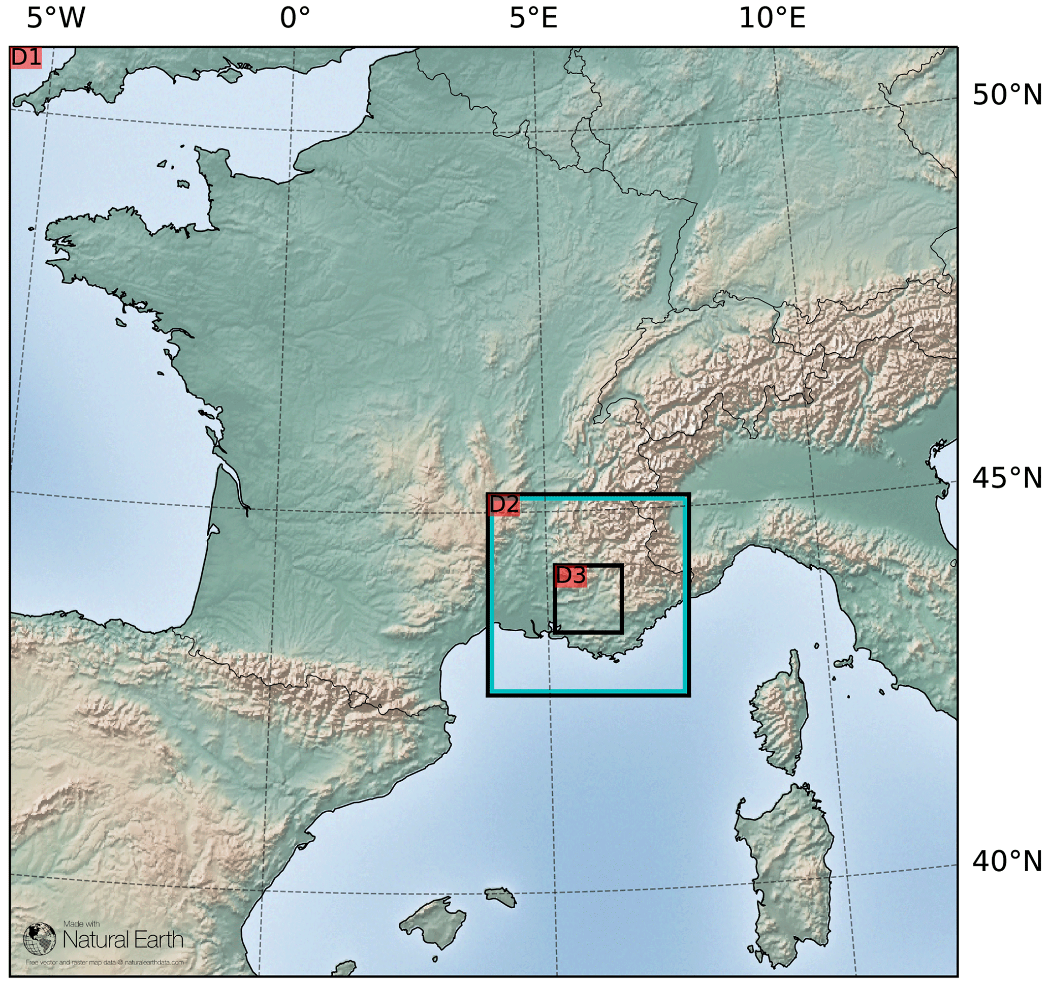
Figure 1Representation of the three nested domains of the WRF model. The blue square represents the 288×288 grid cell area described in Sect. 2.3.
2.2 Training data
The objective is to downscale the 9 km resolution WRF low-level wind forecasts (called WRF LR, for low resolution, in the following) towards a 1 km resolution over an area corresponding to the D3 domain. The 1 km WRF forecast (called WRF HR, for high resolution, in the following) is considered to be the target used to train the statistical models. The wind under consideration throughout this paper is taken at 10 m above the ground.
Wind variables, as well as many other variables, from the WRF LR forecasts are used as predictors for the CNNs: wind components (u for the eastward component, v for the northward component), wind direction (in degrees, both in the ranges of [0;360], and [180;540]) and its cosine and sine, and wind speed; basic meteorological parameters (2 m temperature and potential temperature, surface pressure, and convective and non-convective precipitation); short-wave and long-wave radiation fluxes; and stability-related variables (boundary layer height and friction velocity). Note that numerous predictors are highly influenced by the diurnal cycle (temperature, solar radiation, etc.), which justifies the fact that we did not add explicitly time-related predictors like hours in the day.
Besides, in order to incorporate the geographical context, some HR parameters, called static since they do not vary in time, such as topography (and difference between the LR and HR topography) and a land–sea mask, are added to the list of predictors. Moreover, following the recommendations of Dujardin and Lehning (2022), slope and aspect (orientation of the slope) HR fields calculated from the HR topography are added (see Fig. 2).
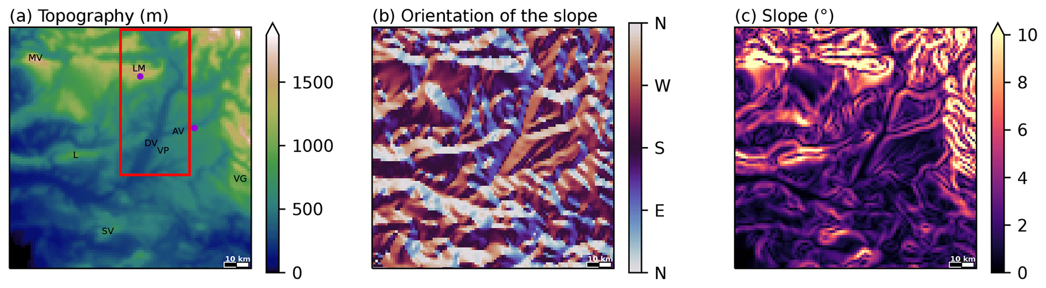
Figure 2Illustration of static predictors for the D3 domain: (a) topography (in m a.s.l.), (b) orientation of the slope and (c) local slope. The red rectangle in (a) shows the area of the plots in Figs. 6, 7 and 8. Letters refer to some topographical sites: MV for Mont Ventoux, LM for Lure mountain, L for Luberon mountain, DV for Durance valley, VP for Valensole plateau, AV for Asse valley, VG for Verdon Gorge and SV for Sainte-Victoire mountain. The two purple dots indicate the locations of the valley site and crest site depicted in Figs. 9 and 10, respectively.
Finally, we added the new predictors introduced by Dujardin and Lehning (2022), which combine wind and topography information, giving insight into wind–topography interactions. More specifically, they calculate a theoretical correction of the wind components in order to represent the speed modification caused by the exposure and sheltering to the wind, as well as the deflection caused by the relief. The reader can refer to Dujardin and Lehning (2022) for more details. Finally, we have a list of 35 predictors (see Table 1) that are all used to train the different CNNs described in the next section.
(see Dujardin and Lehning, 2022)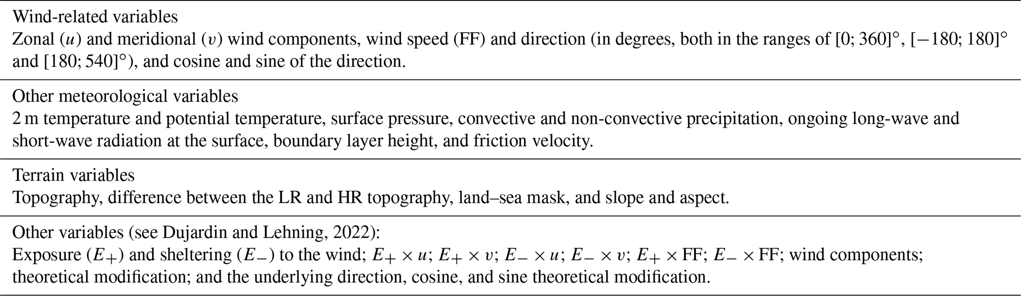
2.3 Convolutional neural network architecture
The objective of a neural network (NN) is to find a mathematical function linking a list of predictors to a list of predictands (considered to be the truth). The function is composed of neurons (a linear combination of input variables transformed by a so-called activation function) interconnected between each other and arranged in layers. Training the NN consists in fitting its function to produce results as close as possible to the truth (the reader can refer to Goodfellow et al., 2016, for more explanations).
Convolutional layers can be introduced in NN when dealing with grid-like data in order to take advantage of the information contained in spatial structures. In these layers, neurons actually correspond to a convolution function which is applied to a limited part of the grid. NNs using such layers are called convolutional neural networks (CNNs).
In this study, we used a U-Net architecture (Ronneberger et al., 2015), which is a fully convolutional network that generates images from images. Its name comes from its U-shaped architecture in which convolutional layers are separated first with pooling layers and then with transposed convolutional layers. The first phase, with pooling layers, reduces the size of images, which is known to capture the context of input images. The second phase, with transposed convolutional layers, increases the size of the contracted images, enabling a precise localization.
The architecture of the CNN used is described in Fig. 3. Before entering the U-Net, the data follow a two-step process. The LR input data are composed of 32×32 grid points with a resolution of 9 km, corresponding to the blue domain represented in Fig. 1. This domain is larger than the D3 domain in order to incorporate information on a larger spatial scale and thus give more information on the regional atmospheric conditions. These data are then interpolated on the HR grid (288×288 grid points with a resolution of 1 km using a bicubic interpolation (the red layer in Fig. 3)) in order to reduce LR grid pattern artifacts in the outputs of the CNN, following which all the predictors are standardized. We used a padding of 1 in order to produce outputs with the same size as inputs although we cropped the 288×288 outputs since we only focus on the 99 km×99 km central area corresponding to the D3 domain. In order to avoid overfitting, we added a batch normalization (Ioffe and Szegedy, 2015) and a drop out (Srivastava et al., 2014) after convolutional layers, and we introduced an early stopping that stopped the learning when the loss function calculated on an independent validation dataset did not improve over 10 successive epochs. The ReLU activation function is applied after each convolutional layer, except for the final 1×1 convolutional layer in order to produce a not-bounded regression. The mean squared error (MSE) is used as loss function. Additional modifications tested are described in the next sections. We used the PyTorch library of Python for the machine learning developments.
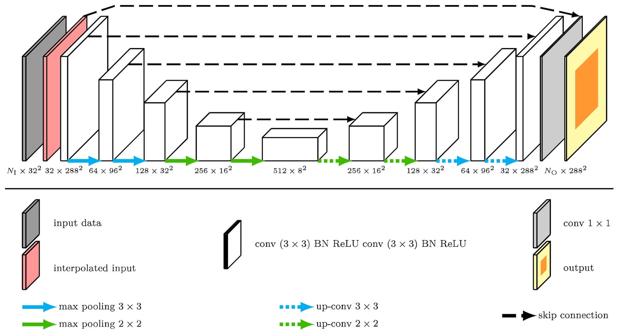
Figure 3Schematic illustrating the architecture of the CNN used in the study. BN stands for batch normalization. The numbers under the different computation blocs indicate the dimension of the data at different stages of the network at the output of the corresponding bloc. NI (=35) and NO (see Table 2) represent the number of input variables and the number of target variables, respectively. On the output, the orange area represents the crop (99×99) from the yellow part (288×288).
2.3.1 Choice of target variables
We are not only interested in the wind speed, as in most studies about wind forecast downscaling, but we also want to calculate the wind direction. However, the direction may be difficult to calculate directly because of its cyclic nature. Circular regression tools are generally based on the von Mises distribution (also called circular normal distribution), but they are challenging to optimize, even if Lang et al. (2020) developed a circular regression tool based on random forests (Breiman, 2001), which simplifies the optimization process. On the other hand, more classic regression approaches, for instance, those based on the estimation of the conditional mean (via the minimization of the mean squared error), seem inappropriate since there is no definition of the mean direction calculated directly on a set of direction values. Despite this, Le Toumelin et al. (2023a) performed a regression that calculated directly the direction, which improved their direction forecast, using a cosine distance as the loss function (see Sect. 2.3.2). We tested their approach via a specific CNN training (this model is called CNNdir hereafter).
Otherwise, the mean direction can be calculated based on its sine and cosine (or wind components in the case of wind data) values (Jammalamadaka and SenGupta, 2001). That is why it is more common to calculate the wind components when using regression tools (Dupuy et al., 2019, 2021a; Höhlein et al., 2020; Miralles et al., 2022; Dujardin and Lehning, 2022) since they carry information on both speed and direction. We apply this approach in this study. Therefore, the CNN outputs two variables aiming at representing the u and v wind components (this model is called CNNu,v hereafter).
Nevertheless, for a given error in any of the two components, the forecast error in the underlying direction varies in terms of the function of the speed (the lower the speed, the higher the error in the direction) and direction. It results that direction errors in lighter winds are artificially less penalized than direction errors in larger winds. Knowing that light winds' directions are difficult to forecast (with a deterministic model) because of their higher spatial and temporal heterogeneity, this strategy reinforces the difficulty. The normalization of the components by the wind speed, which gives the cosine and sine values of the direction (noted and ), is a way to equally penalize all wind speed conditions. We thus tried to forecast these variables (this model is called CNN), although they do not incorporate any information on the speed, which has to be computed in some other way (for instance with the CNNu,v).
2.3.2 Loss function
In our case, the MSE loss produces a negatively biased speed forecast. Dujardin and Lehning (2022) proposed a loss function, inspired by the Pinball function, which is used to make quantile regressions, in order to produce unbiased wind speed predictions when they derive from the components (Eq. 1):
with and being the CNN outputs wind components, and being the target and output speed, and τ and ϵ being two constants. Using values of τ=0.3 and ϵ=4.3 m s−1 (these values were chosen after numerous tests), we obtained an unbiased forecast (model called CNN).
In order to get consistent couples of cosine and sine values when calculating the normalized components, that is to say , we tested a loss function combining the classic MSE and the absolute distance between unity and the sum of squared normalized components (Eq. 2):
with α a weight to balance the two penalty terms. In our case, α=0.2 is the optimal value. For larger values the cosine–sine value couples were globally more consistent but at the expense of the direction forecast.
Another way to get consistent and values is to calculate one of them, for instance , and derive the other one () based on the relation. However, this formula does not give the sign of , which then has to be calculated in another way. In our test, we used the values and signs from CNN (thus, there is no additional CNN training; instead, this approach has to be seen as a postprocess of the CNN results) to calculate (Eq. 3, model called CNN hereafter). Similarly, we calculated based on the values and sign from CNN (model called CNN hereafter).
Finally, as described in the previous section, the CNNdir is trained using its own loss function (ℒdir), introduced in the study of Le Toumelin et al. (2023a):
with dir and being the target and CNN output directions, respectively. A summary of the tests performed in this study is given in Table 2.
2.4 Wind forecast evaluation
The performance was evaluated by comparing the difference between the target (deterministic 1 km WRF simulation) and the output of the various CNNs. The improvement brought by the CNNs translates as a reduction of the wind field error with respect to the initial 9 km WRF wind field error. The latter is computed on the difference between the deterministic 1 km WRF simulation and the 9 km WRF wind field projected onto the 1 km grid (on the D3 domain) with a bicubic interpolation. Therefore, in the following, WRF LR stands for the 1 km field interpolated from the 9 km WRF forecast.
To evaluate the significance of the results and considering the relatively small size of our dataset, we performed a k-fold cross validation in order to use as much data as possible during the training while evaluating the models over a large period. For each CNN model tested, four (k=4 for the cross validation) training runs were performed, each using 75 % of the dataset for training and the remaining 25 % for testing (there is no overlap of data between the four test sets, and the test and training sets are completely independent). By combining the results of the four training runs, applied to the four different test sets, we obtain a test dataset covering the entire period available. Then, we bootstrapped the test dataset, yielding a distribution for each metric, in order to evaluate their dispersion (Wilks, 2011).
We mostly focused on evaluating the wind speed and direction using classic metrics such as the mean absolute error (MAE) and the mean bias error (MBE). Moreover, we compared the accuracy of the wind speed distribution using the Earth Mover's Distance, also known as the Wasserstein distance (WD). The WD between f and , two discrete histograms with samples on N bins and normalized values (in the sense that ), is defined as follows:
where F and are the cumulative histograms of f and . For the direction distribution, we used a modified version called circular Earth Mover's Distance suited to circular variables (Rabin et al., 2008) defined as follows:
where (the definition is similar for through replacing f with ):
Finally, we evaluate the spatial heterogeneity of the wind field by calculating the standard deviation of the speed and direction fields for each of the 29 036 map samples (one value per sample). For the direction, which is a circular variable, we used the Yamartino (1984) method (Eq. 7):
with
2.5 Computational considerations
The training of each CNN on a NVIDIA GeForce GTX TITAN V graphics processing unit (GPU) lasts around 4 h, but once fitted, it takes only a few seconds to process a lead time of one simulation using one of the CNNs listed in Table 2 in the same GPU, which is valuable considering that operational LR forecasts are available several hours ahead, whereas a dynamical downscaling performed with WRF would require hours of computation.
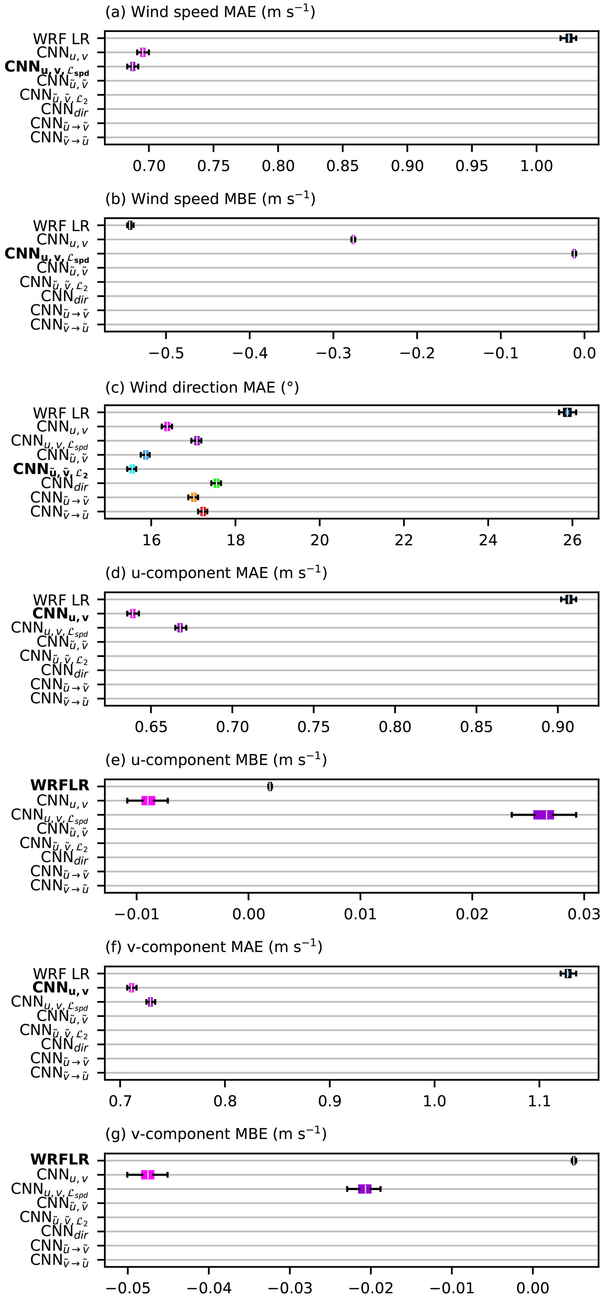
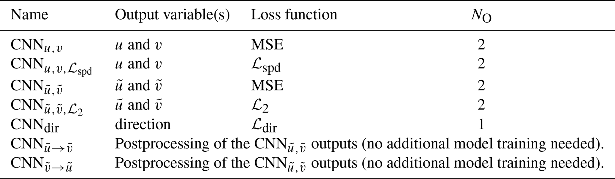
Figure 4Summary of performance for the different models – (a) wind speed MAE, (b) wind speed MBE, (c) wind direction MAE, (d) u MAE, (e) u MBE, (f) v MAE and (g) v MBE. For each metric, the best-performing model label is written in bold type.
3.1 Overall performance of the models
A summary of performance for all the downscaling models is given in Fig. 4. All the CNNs reduce the MAE of the direction and speed, as well as the wind speed bias compared to WRF LR forecasts. However, the bias in the wind components, which is close to zero in WRF LR, is slightly degraded after the downscaling but remains low for all the CNNs (in the range m s−1).
Concerning the wind speed, the CNN is better than the other CNNs, especially for the correction of the negative bias, which is reduced to −0.01 m s−1, demonstrating the ability of the ℒspd loss function to reduce the bias. However, it has one of the worst performances of all the CNNs in terms of the direction and the components (largest MAE values), meaning that the speed improvement occurs at the expense of a degradation of the forecast of the couple of components.
Concerning the direction, all the CNNs greatly improve the performance with respect to the LR forecast, with a reduction in MAE on the order of 10∘. The CNN achieves the best performance. We detail the performance of the different direction forecasts in Fig. 5. In Fig. 5a, we compare the MAEs of the direction according to the wind direction (as computed by WRF HR). The point of this figure is not to focus on the evolution of the MAE in terms of the function of the direction for a given model since many factors should be considered (for instance, the MAE is lower for the northwesterly and southeasterly winds because of the higher occurrence of high speeds for which the direction is easier to forecast). Instead, we analyze the differences, for a given direction, between the different models. The CNN and CNN are really close, while the CNNu,v reaches slightly higher values for southerly winds for unidentified reasons. But above all, the CNNdir behaves singularly, with larger MAE values for winds coming from the NW and NE quadrants, while they are close to the other CNNs for the SW and SE quadrants. This is related to an under-prediction of northerly winds, as illustrated in Fig. 5b, which could result from an artifact around the 0–360∘ numerical discontinuity in the wind direction. It seems that Le Toumelin et al. (2023a, their Fig. 4e) experienced the same issue (important underestimation of the occurrence of northerly winds), possibly with the same consequence for the wind direction MAE, which confirms that calculating the direction as a direct output is not appropriate, as already explained in Sect. 2.3.1. Besides, calculating and without any constraint on the couple they form leads to important inconsistencies ( should be equal to 1 but is underestimated most of the time; see Fig. 5c), which are partly corrected when using the ℒ2 loss (with more values close to 1), together with a slight improvement in the direction forecast. On the other hand, the post-processing of the CNN outputs in order to get and values that respect the equality (CNN and CNN) deteriorates the direction forecast, suggesting that inconsistencies between the couples of and reduce direction errors somehow. Finally, the geographical difference in MAE between the CNN and the CNNu,v (Fig. 5d) indicates that the improvement is not homogeneously spread over the domain but mainly occurs over regions featuring lighter winds on average, generally corresponding to valleys. This behavior was expected since the calculation of the normalized components artificially increases the weight of the direction errors in the lighter winds with respect to the calculation of u and v, as explained in Sect. 2.3.1.
Figure 5(a) MAE in wind direction according to the wind direction from the HR dataset. (b) Polar distributions of the directions computed by the different models. In (a) and (b), the results of CNN, CNN and CNN are not represented in order to make the figures more readable and because their performance in terms of the direction is lower. (c) Distribution of values for CNN and CNN. (d) Difference in MAE in the wind direction between CNN and CNNu,v (negative values mean that CNN performs better, while positive values mean that CNNu,v performs better).
In conclusion, there is no one CNN that outperforms the others. Compared to the classic approach (CNNu,v), the modifications improved either the direction or the speed but not at the same time. Finally, the best overall performance can be obtained by the combination of CNN for the calculation of the speed and CNN for the direction. In the following, CNN results refer to such a combination of post-processing results.
3.2 Wind field characteristics
Before evaluating the downscaling's overall performance, we illustrate the forecast improvement for two selected cases over a limited area of the D3 domain, which is interesting since it encompasses important ridges (e.g., the Lure mountain) and steep local valleys in its northern part and a smoother topography in its southern part, with the wide Durance valley crossing the area from the north towards the south (see the location of the area in Fig. 2a and its topographical characteristics in Fig. 6). The results for the two cases are presented in Figs. 7 and 8, respectively. These figures are composed of six panels split into two rows. There is a classical representation of wind forecasts in the top row (WRF LR (a), WRF HR (b) and CNN (c)) in which the wind is represented with arrows. The bottom row shows the forecast errors of WRF LR (d) and the CNN (f), as well as the correction of the CNN with respect to WRF LR (e): the longer the arrows, the larger the error and/or difference, while the color of the arrows represents the speed error and/or modification. Therefore, in panels (d) and (f) (respectively, (e)), small white arrows indicate a good forecast (respectively, a slightly modified forecast), whereas long white arrows indicate important errors (respectively, important modifications) in direction associated with low-speed errors (respectively, small modifications). Long red and blue arrows in panels (d) and (f) indicate over- and underestimated speeds associated with either a good direction forecast if the orientation of arrows in the WRF LR (panel a) or CNN (panel c) forecast is the same (modulo 180∘), as in the error of forecast (panels d or f), or a bad direction forecast otherwise. The same logic applies to panel (e) for the correction by the CNN.
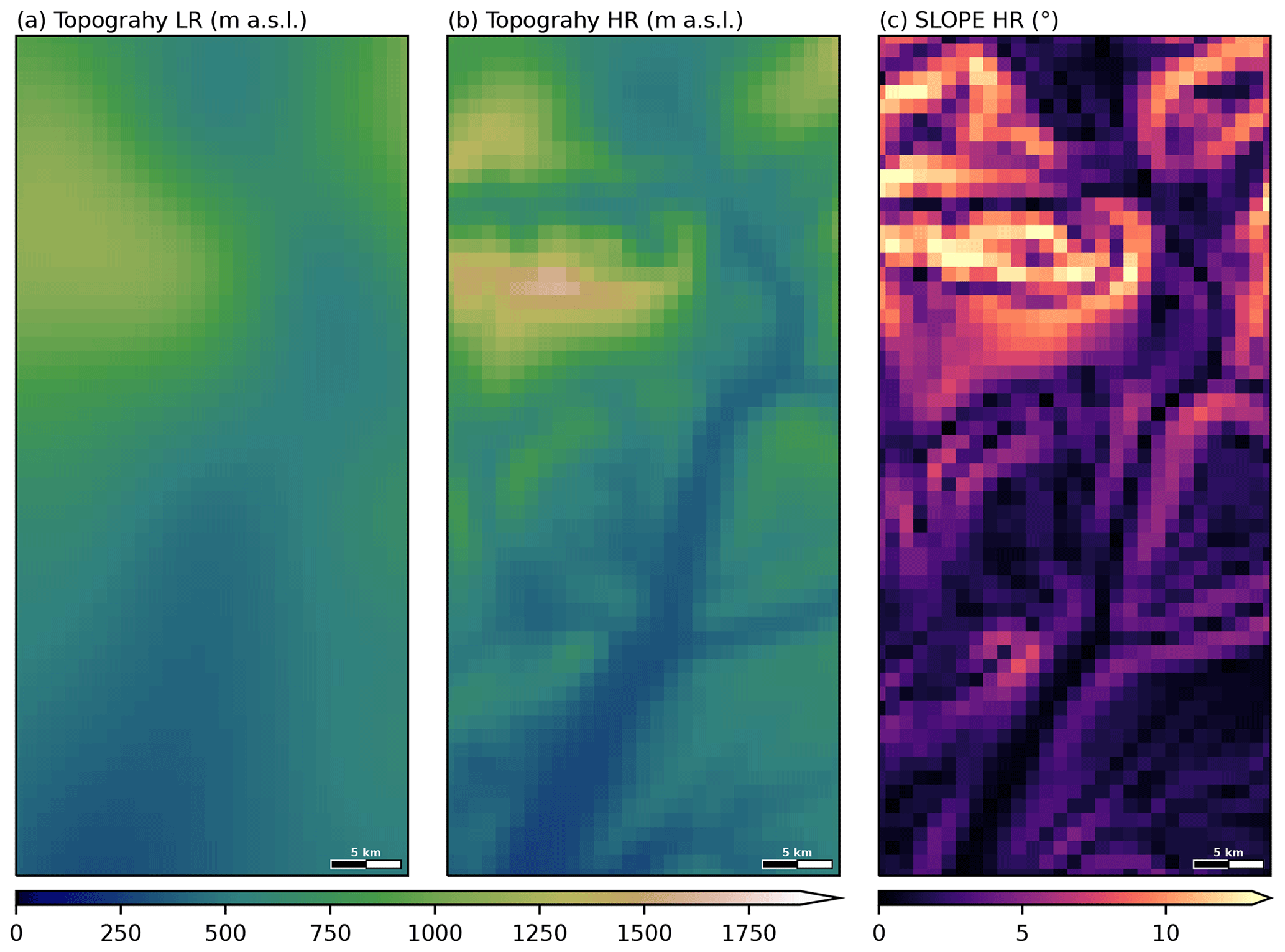
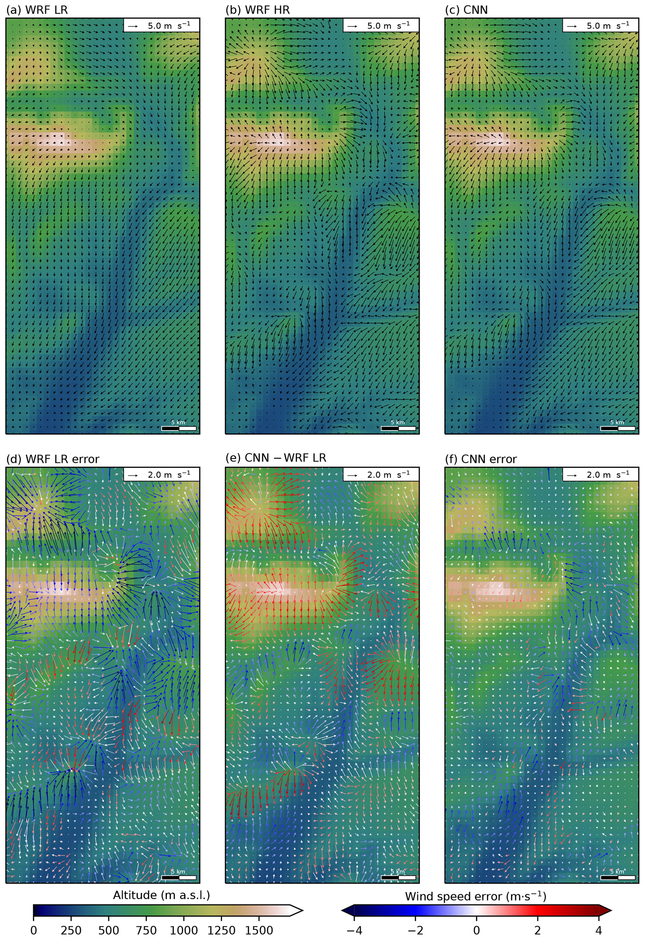
Figure 7Situation of 6 January 2021 at 07:00 UTC (simulation starting at 00:00 UTC on 5 January 2021, lead time 31 h). The area corresponds to the red rectangle in Fig. 2a. Horizontal wind computed by (a) WRF LR, (b) WRF HR and (c) the CNN. Panels (d) and (f) represent the errors corresponding to the wind fields represented in (a) and (c), respectively. Panel (e) represents the vector difference between panels (c) and (a). In panels (d), (e) and (f), the color of the arrows indicates the error or difference in wind speed.
In Fig. 7, the meteorological situation corresponds to a calm night with a weak synoptic forcing. The HR forecast wind field (Fig. 7b) has a high spatial heterogeneity for both speed and direction, resulting from typical topography-dependent features under stable stratification, such as channeled valley winds and downslope winds, e.g., in the northern part of the domain, as well as around less steep hills, e.g., in the southern part of the domain. The LR forecast (Fig. 7a) also features valley and downslope winds but in relation to its LR topography (Fig. 6a), that is to say a single wide and flared valley, bending around the only main ridge resolved in the northwest part of the area. This results in important errors in terms of direction and speed around all the unresolved topographical features (Fig. 7d). The CNN output is very different from the LR wind field over the whole area (long arrows in Fig. 7e), with important speed and/or direction modification. The downscaled wind field (Fig. 7c) appears to be very close to the HR field, with a good representation of all the topography-dependent features, which is confirmed by the errors which are generally very low over the whole area (Fig. 7f).
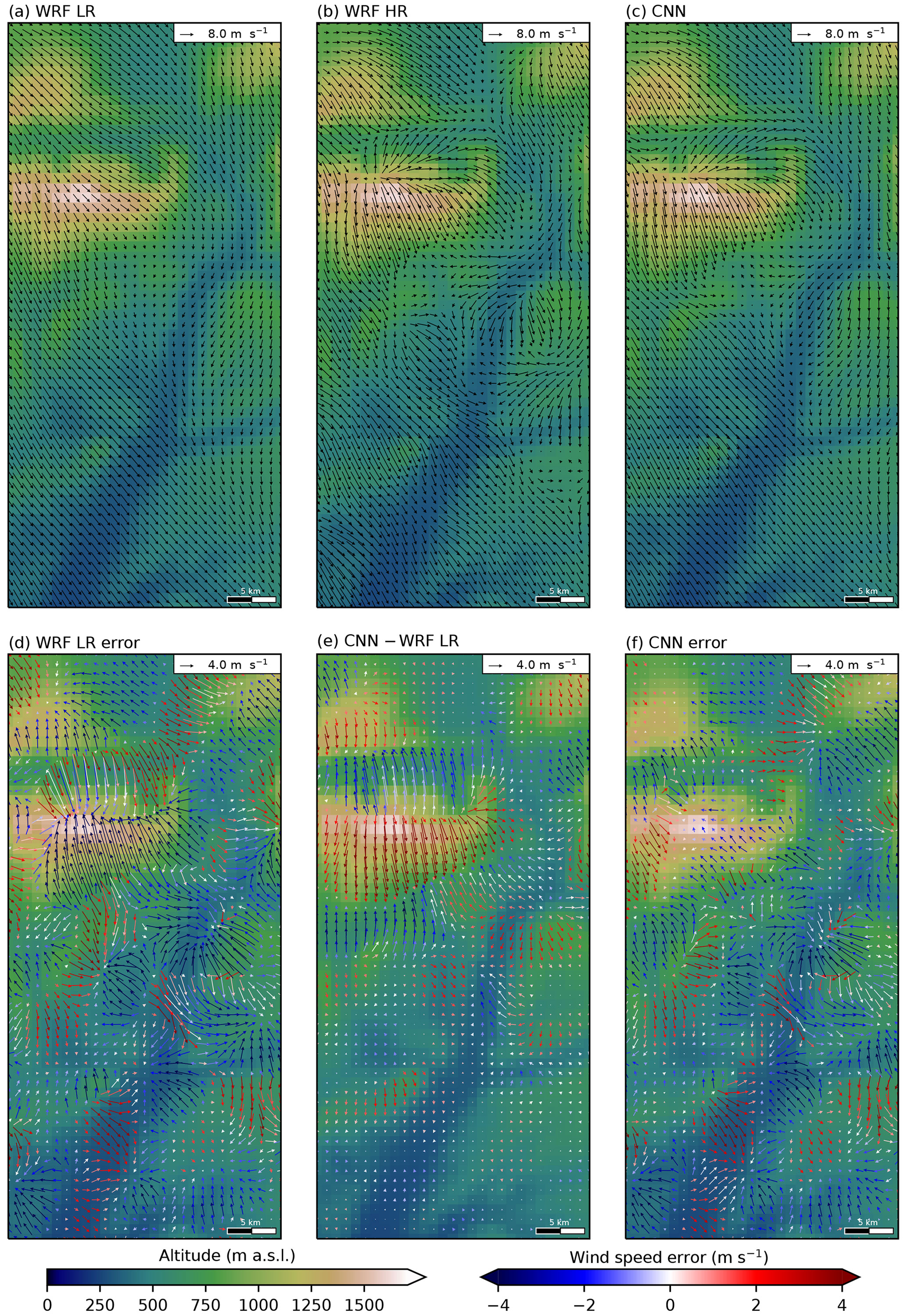
Figure 8Same as Fig. 7 (only the scales of the arrows differ) for the situation of 13 January 2021 at 13:00 UTC (simulation starting at 00:00 UTC on 11 January 2021, lead time 61 h).
The meteorological situation presented in Fig. 8 corresponds to a Mistral (regional wind) event, characterized by northwesterly winds at the synoptic scale over the area considered. Over the southern part of the domain, the HR wind field (Fig. 8b) shows a moderate variability with slight deflections and variations in speed around small-scale reliefs (acceleration over ridges and leeward deceleration). The LR forecast (Fig. 8a) does not represent these topographical features since local topography vanishes at the 9 km resolution. The wind field is therefore very homogeneous, with small direction changes and hence an overestimation of leeward speeds and an underestimation windward (Fig. 8d). The CNN only marginally corrects the LR forecast over this area (small arrows in Fig. 8e). The deflection around reliefs (Fig. 8c) and the leeward deceleration and ridge acceleration (red arrows windward and blue arrows leeward in Fig. 8e) are only partially represented, resulting in significant errors remaining after downscaling (Fig. 8f).
Over the northern part of the domain, the HR wind field (Fig. 8b) is much more impacted by the topography (which features deeper valleys and hills). It results in a flow channeling in narrow valleys, deflections around main hills and a large acceleration over the main ridges. The LR wind field (Fig. 8a) presents features constrained by the highest ridge (the Lure mountain), which is still represented even at the 9 km resolution, with a notable deflection around it, as well as a deceleration on the leeward side. However, deflection and acceleration are lower than those in the HR field, which translates as important errors in the speed over the relief (Fig. 8d). Moreover, topographic effects by small hills and valleys are not represented, which generates large direction and speed errors (Fig. 8d). The correction brought by the CNN is more important over this area (long arrows in Fig. 8e) than over the southern area, allowing one to correctly represent the topographical features present in the HR wind field.
To summarize, the CNN learned the characteristics of the interaction between wind and topography under weak synoptic forcing and under strong wind conditions even if, for the latter, the corrections over local and thin topographical elements are moderate. In the following section, we analyze whether these improvements can be generalized to the whole period.
3.3 Wind climatology at specific sites
We begin this wind climatology with the description of results for two sites featuring very different characteristics, namely a valley site (Fig. 9) and a crest site (Fig. 10). The location of these sites is indicated in Fig. 2a. We picked these two sites as illustrations because valleys and crests are the most difficult locations for wind forecasts.
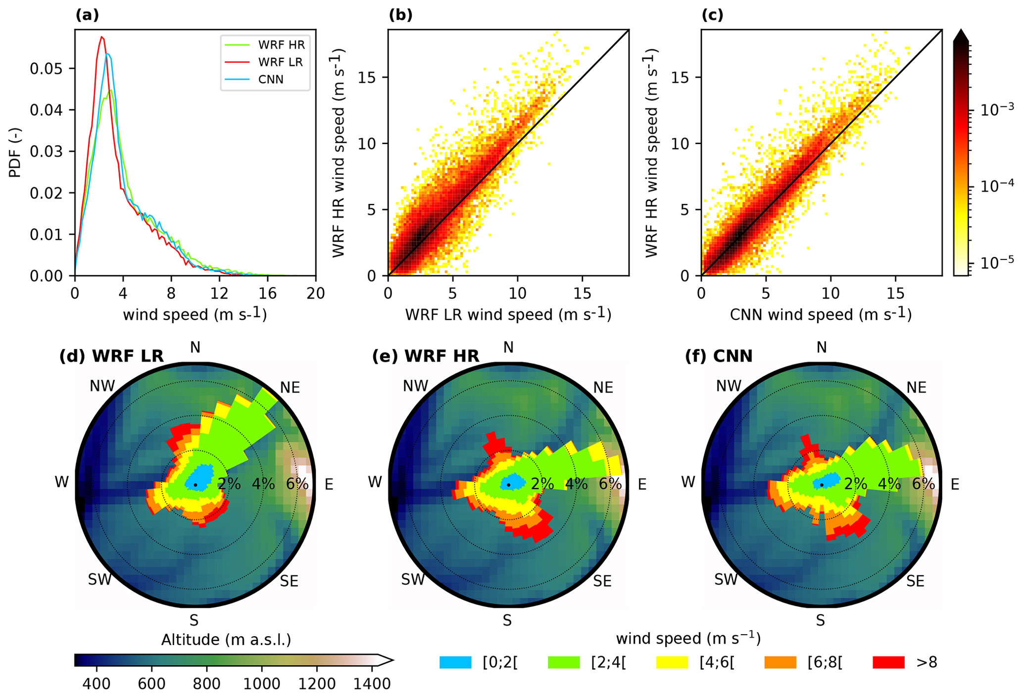
Figure 9Comparison of wind climatology (calculated for our dataset, that is to say from 24 December 2020 to 5 May 2022) between WRF HR, WRF LR and the CNN in a single grid cell in a valley (see purple dot in Fig. 2a for the exact location). (a) Comparison of wind speed probability density functions. (b) Density scatter plot comparing wind speeds from the HR and LR forecasts. (c) Same as (b) for the comparison between the HR forecast and the CNN. Panels (d), (e) and (f) show wind roses of the WRF LR, the WRF HR and the CNN, respectively. The colors of the wind roses represent the wind speed, and the background in the disks represents the topography within a radius of 15 km around the valley site.
The valley site features two different kinds of winds (Fig. 9e). Firstly, there are winds greater than 6 m s−1, which are mainly oriented northwesterly and southeasterly, corresponding to Mistral events and cloudy or rainy weather, respectively, the directions of which are not very dependent on the local topography (important large-scale forcing). These winds are well reproduced in the CNN (Fig. 9f) and reasonably well in WRF LR (Fig. 9d), although the northwesterly winds are more dispersed. Moreover, there is a negative bias in speed associated with these winds in WRF LR (Fig. 9b), which is only marginally corrected by the CNN (Fig. 9c). Secondly, there are west–southwesterly and east–northeasterly winds corresponding to up-valley and down-valley winds, respectively, which are highly dependent on the local topography. Both WRF LR and the CNN correctly predict the up-valley winds. However, WRF LR fails to predict the down-valley winds, which are rotated counterclockwise by approximately 45∘ due to the southwesterly slope of the LR topography at this place (which is consistent with explanations of Fig. 7a), contrarily to the CNN which correctly represents them. Therefore, those winds correspond to downslope winds in both models. Finally, there is an overrepresentation of winds lower than 3 m s−1 in WRF LR, which is only marginally corrected by the CNN (Fig. 9a).
The wind at the crest site features two major orientations, slightly dispersed around the northerly-to-northeasterly and southerly directions (Fig. 10e), mainly resulting from large-scale flow forcing. The WRF LR wind rose also presents a bi-modal distribution that is rotated slightly counterclockwise and has a higher scatter for the southeasterly winds (Fig. 10d). The comparison of the probability density functions of WRF LR and WRF HR (Fig. 10a) highlights a large disagreement, with an overestimation (respectively, underestimation) of the occurrence of lighter (respectively, stronger) winds in WRF LR, which is generalized to all the directions according to Fig. 10d and e. This is consistent with the results depicted in Fig. 8 (underestimation of the ridge acceleration effect). The CNN corrects both the speed and direction (Fig. 10a, c and f). The probability density functions of the CNN and WRF HR are very close, even for strong speeds (whereas WRF LR is unable to predict any wind speed over 15 m s−1 at this site), and the corresponding wind roses look very similar for all directions.
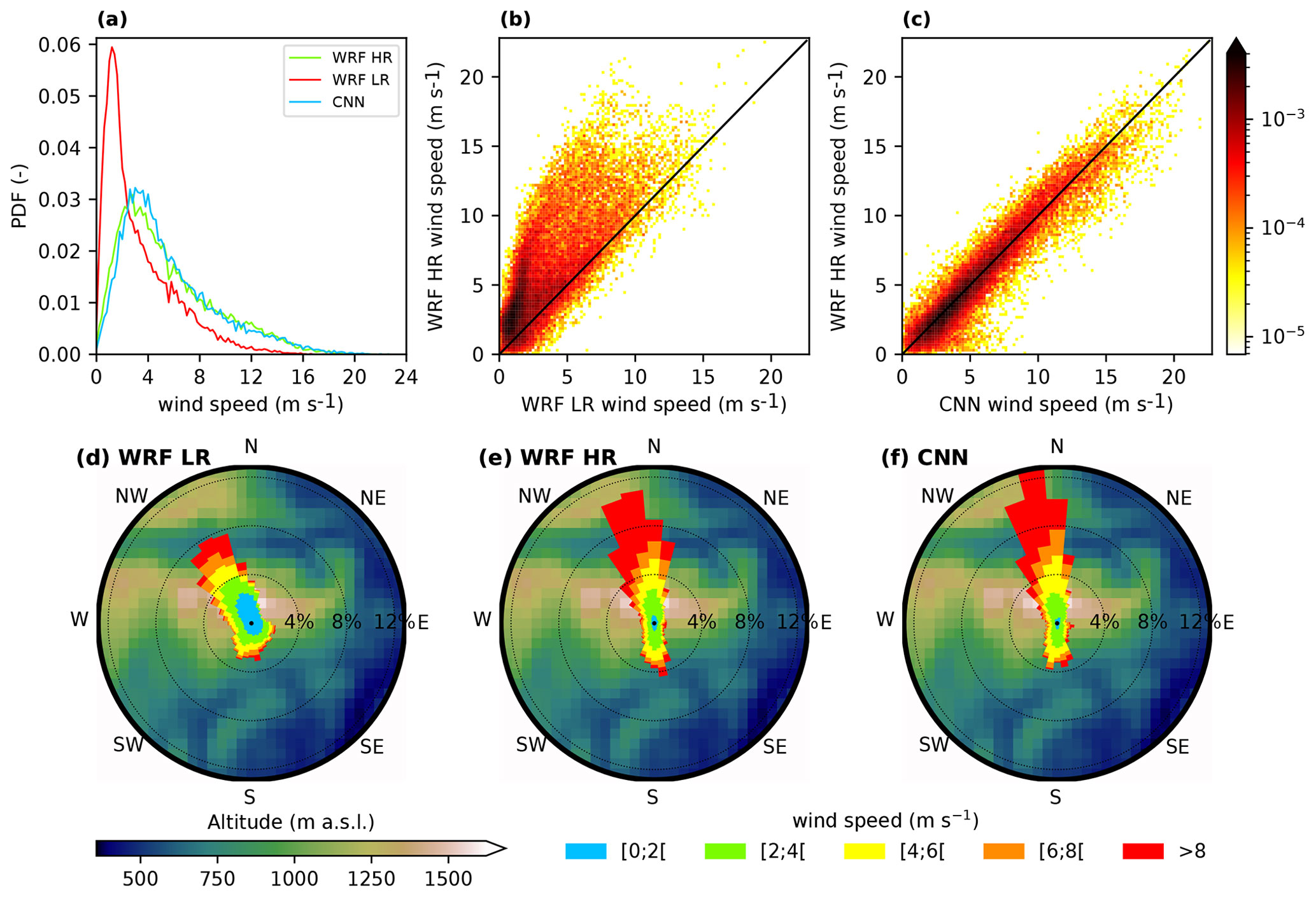
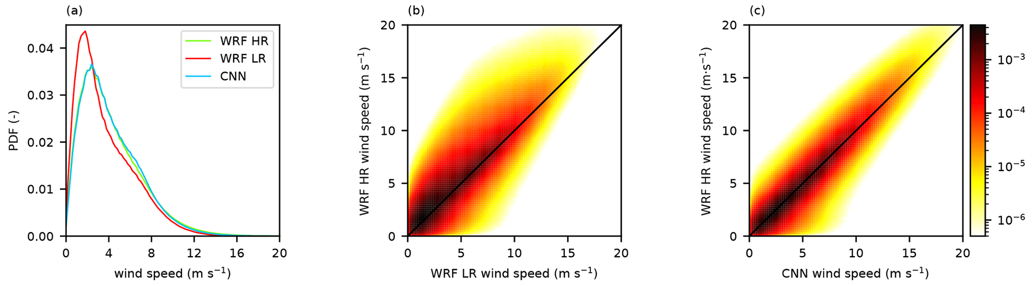
Based on those results, it seems that some of the conclusions made upon the analysis of Figs. 7 and 8 (better representation of the ridge acceleration and the channeling in valleys) can be generalized to the whole period. Moreover, there is a global improvement of the wind speed climatology over the whole domain (Fig. 11). The probability density functions for the CNN and WRF HR are very close (Fig. 11a), while for WRF LR, winds under 3 m s−1 were too frequent (and therefore winds over 3 m s−1 were too rare). The scatter plots (Fig. 11b and c) also demonstrate a better agreement after downscaling, with a concentration of data around the x=y line. We will now investigate whether the results illustrated in Figs. 9 and 10 could be generalized to the other areas of the domain.
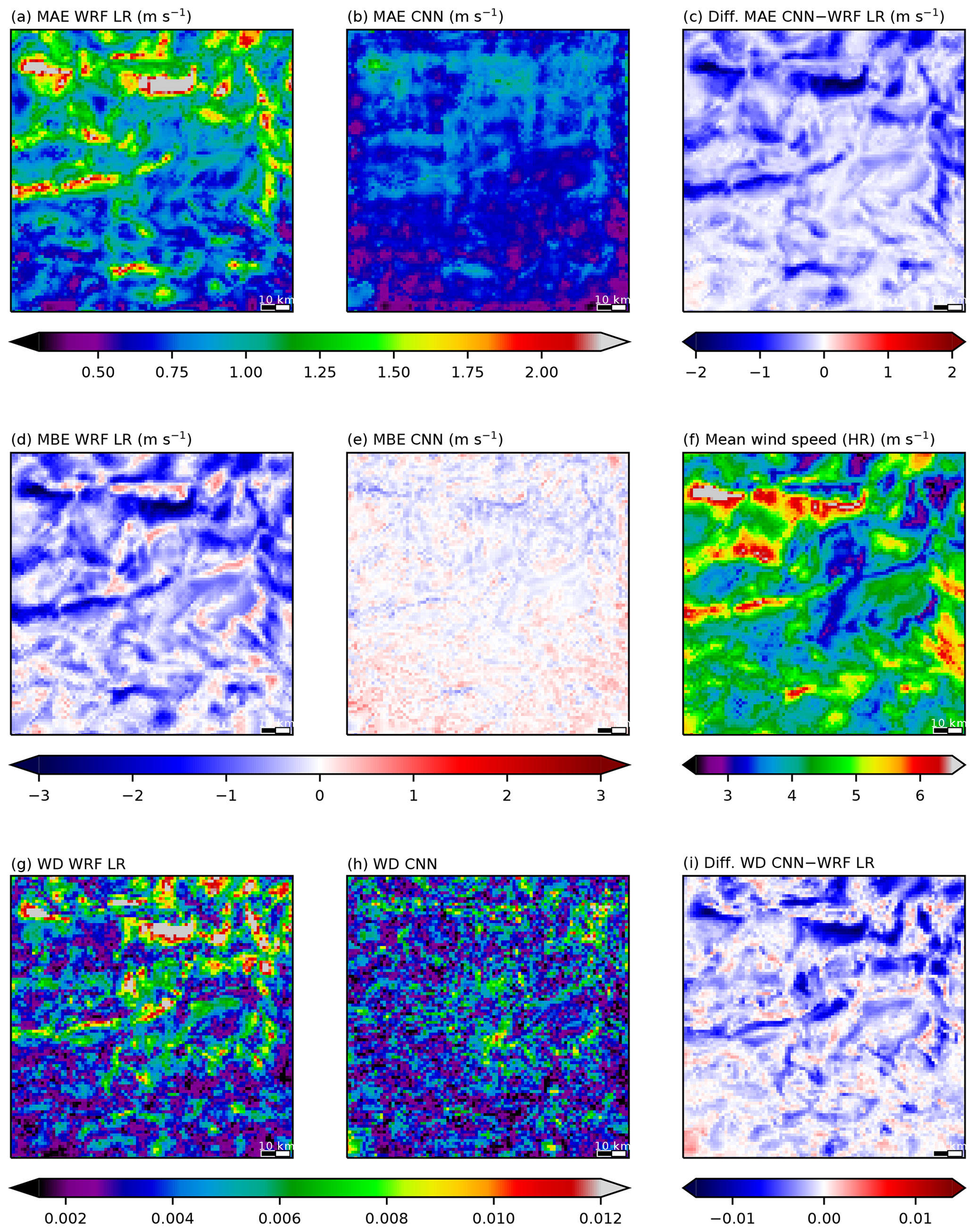
Figure 12Summary of wind speed metrics averaged over the whole period available (from 24 December 2020 to 5 May 2022). Mean absolute error (MAE, a, b), mean bias error (MBE, d, e) and Wasserstein distance (WD, g, h) for the WRF LR forecast and the CNN, respectively. Panels (c) and (i) show the modification brought about by the CNN with respect to WRF LR (negative values for improvements) in terms of the MAE and WD, respectively. Panel (f) shows the mean wind speed calculated from the HR forecast.
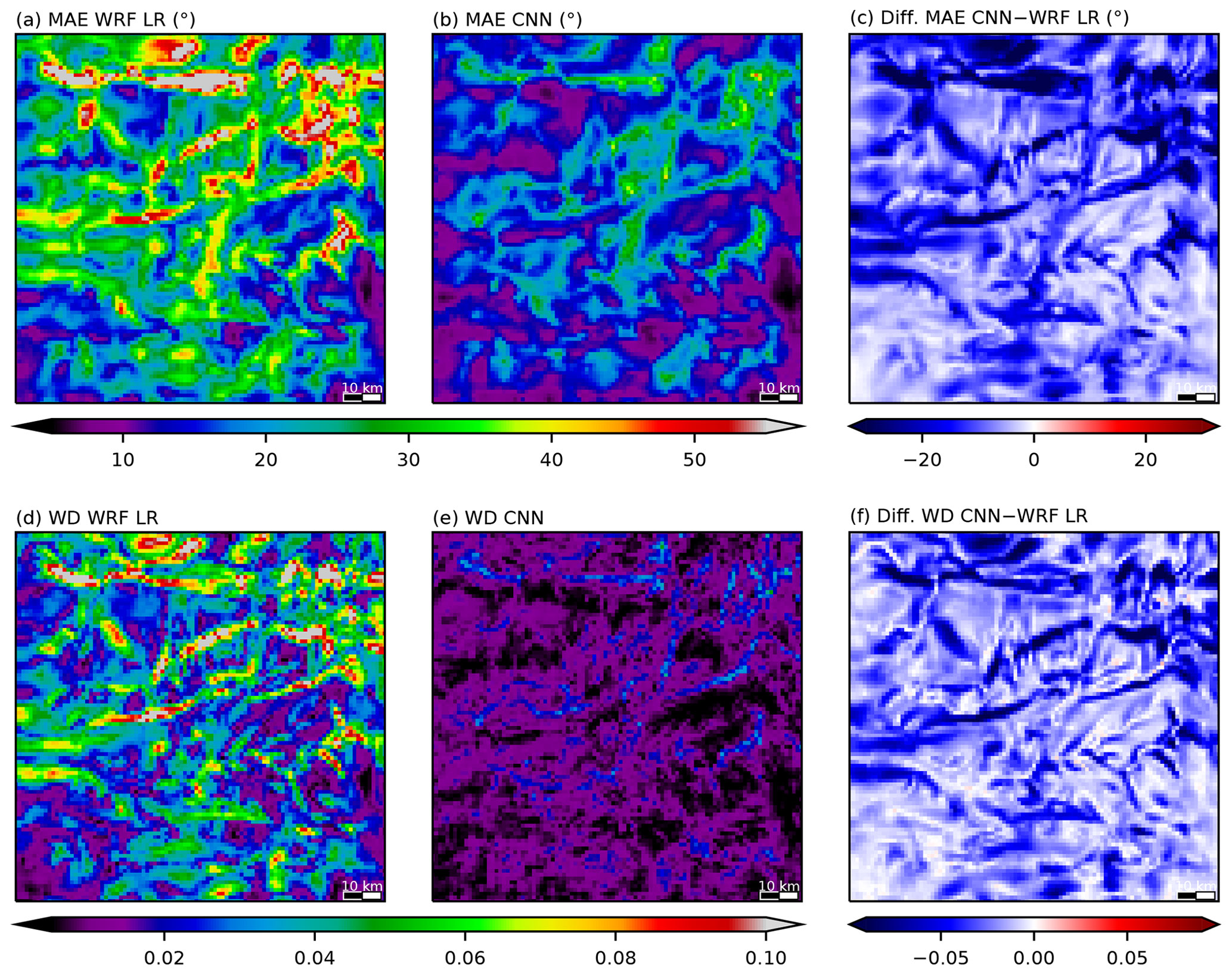
Figure 13Same as Fig. 12 for wind direction metrics and restricted to the MAE (a, b, c) and the WD (d, e, f).
First of all, the mean speed (over the whole period of simulation) from the HR WRF forecast (Fig. 12f) features some expected patterns related to the topography, such as maxima over the highest topographical elements (ridge acceleration) and minima in valleys (sheltering). The WRF LR mean speed is generally underestimated over a large part of the domain (Fig. 12d), resulting in a global MBE of −0.55 m s−1 (see Fig. 4b), with the largest negative biases corresponding to crests. Indeed, the ridge acceleration (see the mean wind speed maxima from WRF HR in Fig. 12f over the Mont Ventoux, the Lure mountain, the Luberon mountain, etc.) is underestimated in WRF LR, resulting in large negative bias values (Fig. 12d). This is consistent with the results over the crest site depicted in Fig. 10. The CNN is able to reproduce the features of the mean wind speed since the MBE is low over most of the domain (Fig. 12e), resulting in a global MBE close to zero (see Fig. 4b).
In WRF LR, the largest MAE values are related to the largest topographic features: high mountains for the speed, where the ridge acceleration is the most important (Fig. 12a), and valleys for the direction, where the channeling cannot be represented without a fine description of the topography (Fig. 13a). The CNN either reduces or at least does not degrade the MAE over the main part of the domain (the only exception being in the southwestern corner, which corresponds to a pond area) for both the speed and direction, with larger improvements (in dark blue in Figs. 12c and 13c) corresponding to regions originally featuring the largest errors in WRF LR.
The WD results indicate that, in WRF LR, the wind climatology is the worst either over the crests for the speed (Fig. 12g), resulting from the large underestimation of ridge acceleration, or in the valleys for the direction (Fig. 13g), resulting from a lack of channeling, which is consistent with the MAE results. The improvement in wind direction brought about by the CNN is translated into a very similar appearance of the MAE (Fig. 13c) or WD (Fig. 13f) field. For the wind speed, there is no similar consensus between the two metrics: the overall structures of the improvement field resemble each other for the MAE (Fig. 12c) and WD (Fig. 12i), but there are local differences, with some spots even reflecting a degradation of the performance evaluated by the WD, as revealed by a few red cells in Fig. 12i. Note that the corresponding MAEs (Fig. 12c) are not degraded at these places. Therefore, from a climatological point of view, WRF LR has mostly a direction issue in valleys and mostly a speed issue over crests, which is consistent with the results of Figs. 9 and 10, and these shortcomings are well corrected by the CNN.
3.4 Diurnal cycle
In this section, we examine how the different metrics evolve according to the time elapsed since the launch of the daily simulations. The results, shown in Fig. 14, represent the average of all the simulations used. Concerning WRF LR, the MAE exhibits a clear diurnal cycle for both the speed (Fig. 14a) and the direction (Fig. 14c), with higher values during the night. This can be explained by the fact that, under stable nocturnal conditions, flows are highly dependent on the local topography, resulting in a high spatial heterogeneity (green lines in Fig. 14b and d for the speed and direction, respectively). After downscaling, the MAE is reduced for all times, and its diurnal cycle remains, although its magnitude is reduced due to a greater improvement during the nighttime when the higher errors were encountered. The nocturnal evolution of the MAE generally exhibits two maxima, at the evening and morning transitions (even if this effect is smoothed on the graphic due to seasonal effect), except for the MAE of the direction in WRF LR, which increases slightly towards its maxima reached at the morning transition. Morning and evening transitions are known to be highly difficult periods to forecast, especially for wind parameters which can experience a high temporal variability, which could explain these error maxima.
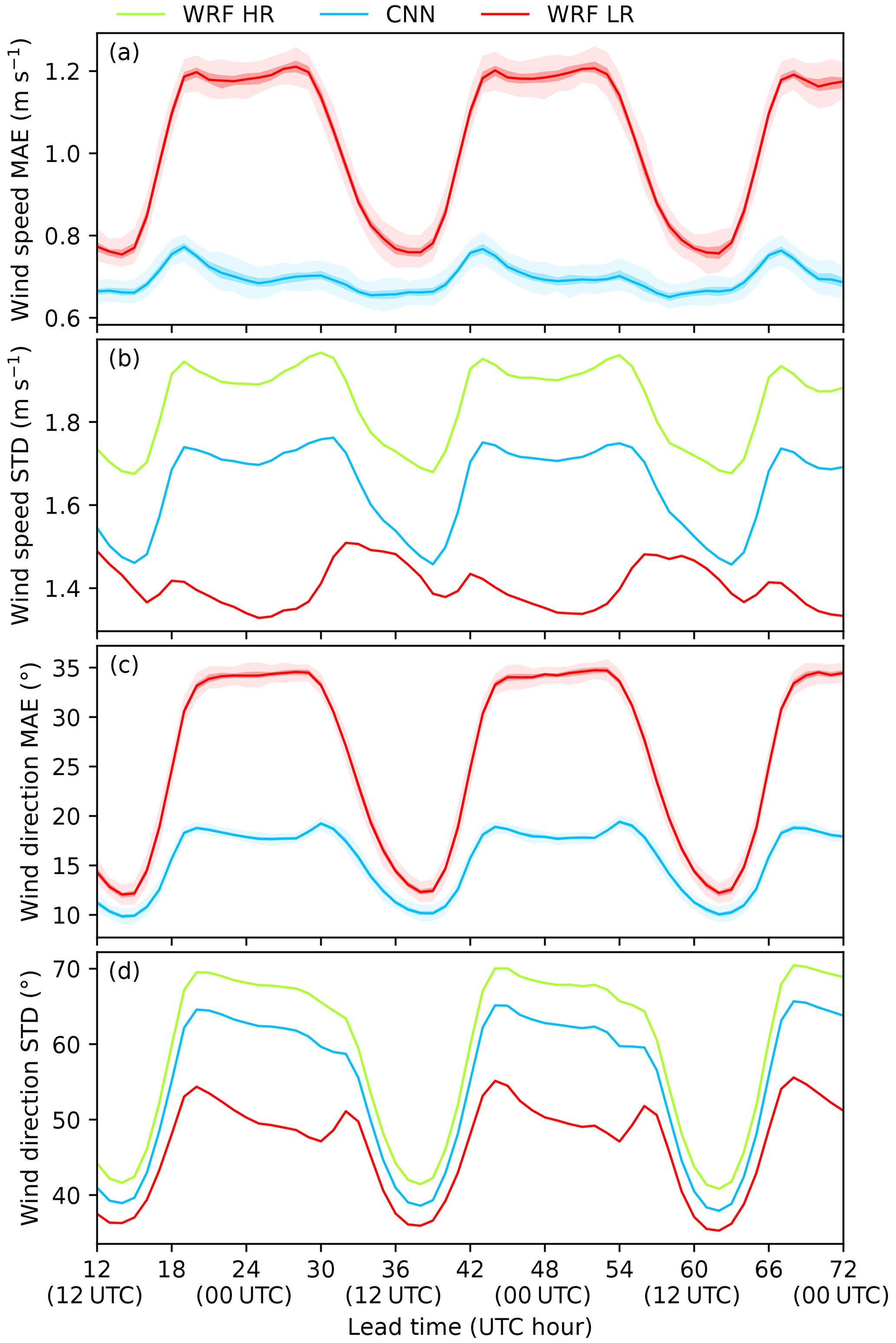
Figure 14Evolution of the MAE for the speed (a) and direction (c) for lead times from 12 to 72 h of the WRF LR forecast (in red) and the CNN (in blue). In these panels, the solid line represents the median value, the dark area is the 25th to 75th quantile interval, and the light areas are the whiskers according to the boxplot construction based on the bootstrap distribution, as explained in Sect. 2.4. Panels (b) and (d) represent the time evolution of the heterogeneity (see Sect. 2.4) for the speed and the direction, respectively.
Note that the lower spatial heterogeneity values encountered in WRF LR in comparison with those in WRF HR, which is consistent with the results presented on Figs. 7 and 8, were expected since the local topography is not resolved in this simulation. The CNN increases the spatial heterogeneity in comparison with WRF LR (also consistent with Figs. 7 and 8) but not enough to reach the values of the HR forecast, demonstrating that the downscaled forecast is still too smooth. A way to improve this issue would be to use a GAN, which is a specific kind of CNN designed to produce very realistic fields (see, for example, Miralles et al., 2022).
CNNs are becoming the most popular deep learning tool, and their specialization for extracting spatial information is well suited to use in atmospheric sciences. Recent studies demonstrated their ability to downscale wind forecasts. In this study, we aimed to move forward in this question by exploring different strategies for downscaling low-level wind forecasts using CNNs, especially regarding the output variables and their associated loss function.
The downscaling was applied to WRF wind forecasts over southeastern France (including the southwestern part of the Alps) from its original 9 km resolution onto a 1 km resolution grid. The 1 km resolution data used for training consist of a series of WRF simulations over a 99 km ×99 km domain, launched for each day of a 16-month period.
Among the approaches tested (i.e., computing the wind components, the normalized components or the wind direction using the MSE loss function in its classical version or with specific adaptations), there is not one that outperforms the others for both the direction and the speed at the same time. Nevertheless, combining two different CNNs dedicated to the direction and speed forecast yields the better overall performance. The best direction forecast is derived from the normalized components, which we found to be more accurate when the loss function is customized by adding a penalty term designed to produce a more physically consistent couple of components. The best speed forecast is derived from the wind components using a modified MSE loss function designed to remove the speed bias, even if the performance for the individual components is degraded.
In comparison with the initial 9 km resolution forecast, the CNN reduced the wind speed bias from −0.55 to −0.01 m s−1, the wind speed MAE from 1.02 to 0.69 m s−1 and the wind direction MAE from 25.9 to 15.5∘. Moreover, some typical topographical features, poorly represented in the LR forecast, are well reproduced in the downscaled wind fields, both for speed (ridge acceleration, leeward deceleration, sheltering in valleys) and direction (deflection, valley channeling). Regarding the diurnal cycle, there is a general improvement in the forecast, especially during the nighttime, stable stratification period, which is the most difficult to simulate. Finally, the downscaling creates a spatial heterogeneity in the wind fields but not at the same level as in the HR forecast. In the future, this issue could be solved by using generative networks, which are specifically designed to produce realistic fields, but with the risk of impacting the overall performance.
We will extend this study by evaluating the performance of the method presented in this paper when applying it over areas other than those where the CNNs have been trained. The first tests already performed have shown an improvement over the initial low-resolution wind fields, although this improvement is much less than that obtained over the area of the present study.
The CNN code has been developed in Python using the Pytorch library. Further information about its content and availability can be obtained from the corresponding author.
No observation data were used in this study. The WRF simulations were run with the open WRF model, version 4.1.2. The outputs of the low- as well as high-resolution simulations (about 3Tb) are stored at CEA. Further information can be obtained from Thierry Hedde (thierry.hedde@cea.fr).
FD developed and implemented the CNN-based models, performed the analyses and wrote the initial version of the paper. PD and TH contributed to the analyses and the writing. TH performed the WRF simulations.
The contact author has declared that none of the authors has any competing interests.
Publisher’s note: Copernicus Publications remains neutral with regard to jurisdictional claims made in the text, published maps, institutional affiliations, or any other geographical representation in this paper. While Copernicus Publications makes every effort to include appropriate place names, the final responsibility lies with the authors.
We thank the Laboratoire d'Aérologie for its support, particularly with regard to GPU computing resources.
This research has been supported by the Commissariat à l'Énergie Atomique et aux Énergies Alternatives (grant no. MRISQ).
This paper was edited by Stéphane Vannitsem and reviewed by two anonymous referees.
Breiman, L.: Random forests, Mach. Learn., 45, 5–32, https://doi.org/10.1023/A:1010933404324, 2001. a
de Bode, M., Hedde, T., Roubin, P., and Durand, P.: Fine-Resolution WRF Simulation of Stably Stratified Flows in Shallow Pre-Alpine Valleys: A Case Study of the KASCADE-2017 Campaign, Atmosphere, 12, 1063, https://doi.org/10.3390/atmos12081063, 2021. a
de Bode, M., Hedde, T., Roubin, P., and Durand, P.: A Method to Improve Land Use Representation for Weather Simulations Based on High-Resolution Data Sets-Application to Corine Land Cover Data in the WRF Model, Earth Space Sci., 10, e2021EA002123, https://doi.org/10.1029/2021EA002123, 2023. a
Dujardin, J. and Lehning, M.: Wind-Topo: Downscaling near-surface wind fields to high-resolution topography in highly complex terrain with deep learning, Q. J. Roy. Meteor. Soc., 148, 1368–1388, https://doi.org/10.1002/qj.4265, 2022. a, b, c, d, e, f, g, h, i, j, k, l
Dupuy, F., Duine, G.-J., Durand, P., Hedde, T., Roubin, P., and Pardyjak, E.: Local-Scale Valley Wind Retrieval Using an Artificial Neural Network Applied to Routine Weather Observations, J. Appl. Meteorol. Clim., 58, 1007–1022, https://doi.org/10.1175/JAMC-D-18-0175.1, 2019. a
Dupuy, F., Duine, G.-J., Durand, P., Hedde, T., Pardyjak, E., and Roubin, P.: Valley Winds at the Local Scale: Correcting Routine Weather Forecast Using Artificial Neural Networks, Atmosphere, 12, 128, https://doi.org/10.3390/atmos12020128, 2021a. a, b
Dupuy, F., Mestre, O., Serrurier, M., Kivachuk Burdá, V., Zamo, M., Cabrera-Gutiérrez, N. C., Bakkay, M. C., Jouhaud, J.-C., Mader, M.-A., and Oller, G.: ARPEGE Cloud Cover Forecast Postprocessing with Convolutional Neural Network, Weather Forecast., 36, 567–586, https://doi.org/10.1175/WAF-D-20-0093.1, 2021b. a
Fiddes, J. and Gruber, S.: TopoSCALE v.1.0: downscaling gridded climate data in complex terrain, Geosci. Model Dev., 7, 387–405, https://doi.org/10.5194/gmd-7-387-2014, 2014. a, b
Goodfellow, I., Bengio, Y., and Courville, A.: Deep Learning, MIT Press, http://www.deeplearningbook.org (last access: 2 November 2023), 2016. a
Harris, L., McRae, A. T. T., Chantry, M., Dueben, P. D., and Palmer, T. N.: A Generative Deep Learning Approach to Stochastic Downscaling of Precipitation Forecasts, J. Adv. Model. Earth Sy., 14, e2022MS003120, https://doi.org/10.1029/2022MS003120, 2022. a
Höhlein, K., Kern, M., Hewson, T., and Westermann, R.: A comparative study of convolutional neural network models for wind field downscaling, Meteorol. Appl., 27, e1961, https://doi.org/10.1002/met.1961, 2020. a, b, c, d, e, f
Ioffe, S. and Szegedy, C.: Batch Normalization: Accelerating Deep Network Training by Reducing Internal Covariate Shift, Proceedings of the 32nd International Conference on Machine Learning, 7–9 July 2015, Lille, France, 448–456, 2015. a
Jammalamadaka, S. R. and SenGupta, A.: Topics in Circular Statistics, World Sci., 1, 1–24, https://doi.org/10.1142/4031, 2001. a
Kruyt, B., Mott, R., Fiddes, J., Gerber, F., Sharma, V., and Reynolds, D.: A Downscaling Intercomparison Study: The Representation of Slope- and Ridge-Scale Processes in Models of Different Complexity, Front. Earth Sci., 10, 789332, https://doi.org/10.3389/feart.2022.789332, 2022. a
Kulkarni, A., Shivananda, A., and Sharma, N. R.: Image Super-Resolution, Apress, Berkeley, CA, 261–295, https://doi.org/10.1007/978-1-4842-8273-1_8, 2022. a
Lagerquist, R., McGovern, A., and Gagne II, D. J.: Deep Learning for Spatially Explicit Prediction of Synoptic-Scale Fronts, Weather Forecast., 34, 1137–1160, https://doi.org/10.1175/WAF-D-18-0183.1, 2019. a
Lang, M. N., Schlosser, L., Hothorn, T., Mayr, G. J., Stauffer, R., and Zeileis, A.: Circular Regression Trees and Forests with an Application to Probabilistic Wind Direction Forecasting, J. Roy. Stat. Soc. C-App., 69, 1357–1374, https://doi.org/10.1111/rssc.12437, 2020. a
Le Toumelin, L., Gouttevin, I., Galiez, C., and Helbig, N.: A two-folds deep learning strategy to correct and downscale winds over mountains, Nonlin. Processes Geophys. Discuss. [preprint], https://doi.org/10.5194/npg-2023-10, in review, 2023a. a, b, c, d, e, f, g
Le Toumelin, L., Gouttevin, I., Helbig, N., Galiez, C., Roux, M., and Karbou, F.: Emulating the Adaptation of Wind Fields to Complex Terrain with Deep Learning, Artificial Intelligence for the Earth Systems, 2, e220034, https://doi.org/10.1175/AIES-D-22-0034.1, 2023b. a, b, c, d, e, f, g
LeCun, Y., Bengio, Y., and Hinton, G.: Deep learning, Nature, 521, 436–444, https://doi.org/10.1038/nature14539, 2015. a
Leinonen, J., Nerini, D., and Berne, A.: Stochastic Super-Resolution for Downscaling Time-Evolving Atmospheric Fields With a Generative Adversarial Network, IEEE T. Geosci. Remote, 59, 7211–7223, https://doi.org/10.1109/TGRS.2020.3032790, 2021. a
Miralles, O., Steinfeld, D., Martius, O., and Davison, A. C.: Downscaling of Historical Wind Fields over Switzerland Using Generative Adversarial Networks, Artificial Intelligence for the Earth Systems, 1, e220018, https://doi.org/10.1175/AIES-D-22-0018.1, 2022. a, b, c, d, e, f, g, h
Rabin, J., Delon, J., and Gousseau, Y.: Circular Earth Mover's Distance for the comparison of local features, in: 2008 19th International Conference on Pattern Recognition, Tampa, FL, USA, 8–11 December 2008, 1–4, https://doi.org/10.1109/ICPR.2008.4761372, 2008. a
Reichstein, M., Camps-Valls, G., Stevens, B., Jung, M., Denzler, J., Carvalhais, N., and Prabhat: Deep learning and process understanding for data-driven Earth system science, Nature, 566, 195–204, https://doi.org/10.1038/s41586-019-0912-1, 2019. a
Ronneberger, O., Fischer, P., and Brox, T.: U-Net: Convolutional Networks for Biomedical Image Segmentation, CoRR, arXiv [preprint], https://doi.org/10.48550/arXiv.1505.04597, 18 May 2015. a
Salameh, T., Drobinski, P., Vrac, M., and Naveau, P.: Statistical downscaling of near-surface wind over complex terrain in southern France, Meteorol. Atmos. Phys., 103, 253–265, https://doi.org/10.1007/s00703-008-0330-7, 2009. a
Schmidli, J., Böing, S., and Fuhrer, O.: Accuracy of Simulated Diurnal Valley Winds in the Swiss Alps: Influence of Grid Resolution, Topography Filtering, and Land Surface Datasets, Atmosphere, 9, 196, https://doi.org/10.3390/atmos9050196, 2018. a
Skamarock, W. C., Klemp, J. B., Dudhia, J., Gill, D. O., Liu, Z., Berner, J., Wang, W., Powers, J. G., Duda, M. G., Barker, D. M., and Huang, X.: A description of the advanced research WRF model version 4, National Center for Atmospheric Research: Boulder, CO, USA, 145, 550, https://doi.org/10.5065/1dfh-6p97, 2019. a
Srivastava, N., Hinton, G., Krizhevsky, A., Sutskever, I., and Salakhutdinov, R.: Dropout: A Simple Way to Prevent Neural Networks from Overfitting, J. Mach. Learn. Res., 15, 1929–1958, 2014. a
Vandal, T., Kodra, E., Ganguly, S., Michaelis, A., Nemani, R., and Ganguly, A. R.: Generating High Resolution Climate Change Projections through Single Image Super-Resolution: An Abridged Version, in: Proceedings of the Twenty-Seventh International Joint Conference on Artificial Intelligence, IJCAI-18, International Joint Conferences on Artificial Intelligence Organization, Stockholm, Sweden 13–19 July 2018, 5389–5393, https://doi.org/10.24963/ijcai.2018/759, 2018. a
Vannitsem, S., Bremnes, J. B., Demaeyer, J., Evans, G. R., Flowerdew, J., Hemri, S., Lerch, S., Roberts, N., Theis, S., Atencia, A., Bouallègue, Z. B., Bhend, J., Dabernig, M., Cruz, L. D., Hieta, L., Mestre, O., Moret, L., Plenković, I. O., Schmeits, M., Taillardat, M., den Bergh, J. V., Schaeybroeck, B. V., Whan, K., and Ylhaisi, J.: Statistical Postprocessing for Weather Forecasts: Review, Challenges, and Avenues in a Big Data World, B. Am. Meteorol. Soc., 102, E681–E699, https://doi.org/10.1175/BAMS-D-19-0308.1, 2021. a
Wagenbrenner, N. S., Forthofer, J. M., Lamb, B. K., Shannon, K. S., and Butler, B. W.: Downscaling surface wind predictions from numerical weather prediction models in complex terrain with WindNinja, Atmos. Chem. Phys., 16, 5229–5241, https://doi.org/10.5194/acp-16-5229-2016, 2016. a, b
Whiteman, C. D.: Mountain Meteorology: Fundamentals and Applications, Oxford University Press, https://doi.org/10.1093/oso/9780195132717.001.0001, 2000. a
Wilks, D.: Chapter 8 – Forecast Verification, in: Statistical Methods in the Atmospheric Sciences, edited by: Wilks, D. S., vol. 100 of International Geophysics, Academic Press, 301–394, https://doi.org/10.1016/B978-0-12-385022-5.00008-7, 2011. a
Yamartino, R. J.: A Comparison of Several “Single-Pass” Estimators of the Standard Deviation of Wind Direction, J. Appl. Meteorol. Clim. 23, 1362–1366, https://doi.org/10.1175/1520-0450(1984)023<1362:ACOSPE>2.0.CO;2, 1984. a
Yang, W., Zhang, X., Tian, Y., Wang, W., Xue, J.-H., and Liao, Q.: Deep Learning for Single Image Super-Resolution: A Brief Review, IEEE T. Multimedia, 21, 3106–3121, https://doi.org/10.1109/TMM.2019.2919431, 2019. a
Zamo, M., Bel, L., Mestre, O., and Stein, J.: Improved Gridded Wind Speed Forecasts by Statistical Postprocessing of Numerical Models with Block Regression, Weather Forecast., 31, 1929–1945, https://doi.org/10.1175/WAF-D-16-0052.1, 2016. a