Quantitative comparison of causal inference methods for climate tipping points

Causal inference methods present a statistical approach to the analysis and reconstruction of dynamic systems as observed in nature or in experiments. Climate tipping points are likely present in several core components of the Earth system, such as the Greenland ice sheet or the Atlantic Meridional Overturning Circulation (AMOC), and are characterized by an abrupt and irreversible degradation under sustained global temperatures above their corresponding thresholds. Causal inference methods may provide a promising way to study the interactions of climate tipping elements, which are currently highly uncertain due to limitations in model-based approaches. However, the data-driven analysis of climate tipping elements presents several challenges, e.g., with regard to nonlinearity, delayed effects and confoundedness. In this study, we quantify the accuracy of three commonly used multivariate causal inference methods with regard to these challenges and find unique advantages of each method: The Liang–Kleeman Information Flow (LKIF) is preferable in simple settings with limited data availability, the Peter–Clark Momentary Conditional Independence (PCMCI) provides the most control, e.g., to integrate expert knowledge, and the Granger Causality for State Space Models is advantageous for large datasets and delayed interactions. In general, data sampling intervals should be aligned with the interaction delays, and the inclusion of a confounder (like global temperatures) is crucial to deal with the nonlinear response to (climate) forcing. Based on these findings and given their data masking capabilities, we apply the LKIF and PCMCI methods to reanalysis data to detect tipping point interactions between the AMOC and Arctic summer sea ice, which imply a bidirectional stabilizing interaction, in agreement with physical mechanisms. Our results therefore contribute robust evidence to the study of interactions of the AMOC and the cryosphere.

1 Introduction

Tipping points have been identified in several core elements of the Earth system, such as the polar ice sheets and the Atlantic Meridional Overturning Circulation (AMOC) (Lenton et al., 2008; Armstrong McKay et al., 2022). These elements are expected to enter tipping processes through destabilizing feedback effects once a respective threshold in forcing has been crossed, directly or indirectly, due to global warming. This threshold-based tipping dynamic is referred to as bifurcation-induced tipping. Noise or the rate of forcing may also lead to a tipping process (Ashwin et al., 2012; Klose et al., 2024). A tipping process is defined by its self-reinforcing dynamics, i.e., even if temperature levels are stabilized above the threshold, the element continuously degrades into a different stable state. This degradation thus becomes difficult to reverse even at lower temperatures, once a tipping point has been crossed for a significant amount of time. For instance, for the Greenland ice sheet, a tipping process would be characterized by continuous melting due to melt elevation feedback, among other factors (Boers and Rypdal, 2021), which would increase global sea levels by several meters (Morlighem et al., 2017). The AMOC is considered to be forced by freshwater (van Westen et al., 2024b; Swingedouw et al., 2022) and warming (Drijfhout et al., 2025; Laridon et al., 2025) in its northern convection regions, and could experience a significant weakening or shutdown due to its salt advection feedback (Vanderborght et al., 2025; Caesar et al., 2018; Boers, 2021; Ditlevsen and Ditlevsen, 2023), with severe consequences for the climate of the Northern Hemisphere and beyond (Jackson et al., 2015; van Westen et al., 2024b; Orihuela-Pinto et al., 2022).

The resilience of tipping elements has thus become a crucial subject within climate science, communication and the surrounding area of policy. Their relevance is underlined by the dedicated chapter on tipping points in the upcoming IPCC report (AR7, Chap. 8: “Abrupt changes, low-likelihood high impact events and critical thresholds, including tipping points, in the Earth system”), large collaborative projects like the Global Tipping Points report (Lenton et al., 2025), and by the recognition of tipping points in the study of economic and social climate change impacts (Trust et al., 2025; Stoerk et al., 2025).

Interactions among tipping elements may further deteriorate the resilience of tipping elements under global warming. The current literature mostly identifies destabilizing interactions (Wunderling et al., 2024), e.g., meltwater of the Greenland ice sheet would weaken the AMOC (Swingedouw et al., 2022; Klose et al., 2024). Research on these tipping point interactions is still in an early stage and even lacking entirely for several hypothesized tipping element interactions. However, some initial work has been conducted using Earth system models of intermediate complexity (EMIC) (Willeit et al., 2023; Kaufhold et al., 2025; Sinet et al., 2025), as fully complex Earth system models are only starting to represent elements like ice sheets and vegetation dynamically.

Statistical methods may be suitable to detect significant directed interactions between variables in dynamic systems. Applying these methods to time series data of (potentially) interacting tipping elements may provide a promising data-driven approach to estimate tipping point interactions without the usage of climate models. Correlation tests are frequently used to analyze variable relationships or interactions, but they do not provide a sufficient theoretical foundation to derive directional causality. Multivariate causal inference methods provide a theoretical derivation of causality from statistical measures and consider networks of variables and their interactions. Several such methods have been developed in the past decades for different assumptions about the underlying processes (Runge et al., 2019a; Camps-Valls et al., 2023). Previous studies have often tested or compared methods under idealized settings with regard to sample availability (Docquier et al., 2024), interaction strength (Runge et al., 2019b; Liang et al., 2025) and/or network complexity (Nogueira et al., 2022; Assaad et al., 2022). Results of causal analysis can also inform the structure or parameterization of models (Debeire et al., 2025). The application of causal methods to model data may in turn serve as an evaluation of the accuracy of the macroscopic behavior emerging from a model (Nowack et al., 2020).

Causal analysis has so far only been applied to climate tipping points directly in a study where the Peter–Clark Momentary Conditional Independence (PCMCI) method was used to detect a stabilizing interaction from the AMOC to the Southern Amazon rainforest (Högner et al., 2025). However, so far there is no systematic assessment of different causal methods applied to synthetic data that displays nonlinear behavior resembling the dynamics of tipping elements and that can be designed to exhibit characteristics typical for Earth observation data.

With this study, we aim to estimate the reliability and robustness of three causal methods in the context of climate tipping elements, which pose some specific challenges:

• As the period of modern observations is short compared to the timescales of tipping elements, the number of available samples is low, often below 1000 (Högner et al., 2025; Kretschmer et al., 2016)

• Interactions between analyzed elements may be weak or highly delayed due to the atmospheric or oceanic transport required to propagate interaction effects (Di Capua et al., 2023)

• Large and dense networks of variables may be of special interest, e.g., due to regional tipping patterns (Runge et al., 2015)

• Global warming influences all climate tipping elements, bringing them closer to their tipping thresholds. Such a background effect may complicate causal analysis by introducing a (potentially nonlinear and noisy) trend to the states of tipping elements.

We therefore conduct experiments to explore the role of the sample size, strength and delay of interactions, and the size, density and confoundedness of the interaction network in the prediction of the network by causal methods. We compare three causal inference methods, selected for their wide use in the literature and their capacity for multivariate analysis in limited datasets (e.g., in contrast to neural network methods, which require much larger datasets): The Liang–Kleeman Information Flow (LKIF) (Liang, 2021), the Peter–Clark Momentary Conditional Independence (PCMCI) (Runge et al., 2019b), and the State Space Granger Causality (GCSS) (Barnett and Seth, 2015). We generate data from a network model of differential equations and rate the detection capabilities of each method quantitatively by comparing the statistically significant detected links with the true constellation of interactions in the underlying model. We derive three core recommendations from our results, which should provide some guidance on the application of causal methods to climate tipping points, especially with regard to the required assumptions on data and the underlying physical system.

We further conduct an applied experiment to demonstrate the usage of the analyzed causal methods on a tipping point interaction between the AMOC and Arctic summer sea ice (ASSI). Freshwater influx and surface temperatures are considered important factors for AMOC stability (Weijer et al., 2019; Petit et al., 2020). Previous results on the interaction of Arctic sea ice and the AMOC are ambiguous (Weijer et al., 2022), as freshwater from Arctic sea ice melt may weaken the AMOC by decreasing buoyancy in the convection regions (Li et al., 2021; Liu and Fedorov, 2022), while sea ice melt may also increase heat loss of the sea surface, thus increasing the buoyancy (Wu et al., 2021). Our interaction study contributes a data-driven perspective to this open question. We conduct appropriate data preprocessing steps (detrending, deseasonalising, spatial filtering), and include Arctic temperatures as a potential confounder. Further, our experiment demonstrates and discusses the selection of PCMCI as the most suitable causal inference method based on application constraints.

This paper is structured as follows: Sect. 2 describes the methodology of our experiments, the utilized causal methods and the data generation process. In Sect. 3, we present the results of our comparative experiments on synthetic data under various conditions expected to be present in physical tipping elements. In Sect. 4, we discuss the results and derive recommendations for the application of causal methods in the study of climate tipping points and their interactions. An applied experiment is presented in Sect. 5, where we apply our recommendations to a hypothesized interaction between the AMOC and ASSI. Section 6 provides conclusions and outlooks for further work.

2 Methods and Data

For our model experiments, data are generated from a network model of nonlinear dynamic equations. The generated time series data are fed into three causal algorithms, each of which determines a graph of significant interactions. Lastly, the predicted graph is compared to the true network model used for data generation as an evaluation of detection accuracy. Figure 1 visualizes this approach. In the following, we first introduce the data generation model, then describe each of the utilized causal methods and their underlying concepts of causality. Lastly, we introduce the metrics of detection accuracy used in the experiments.

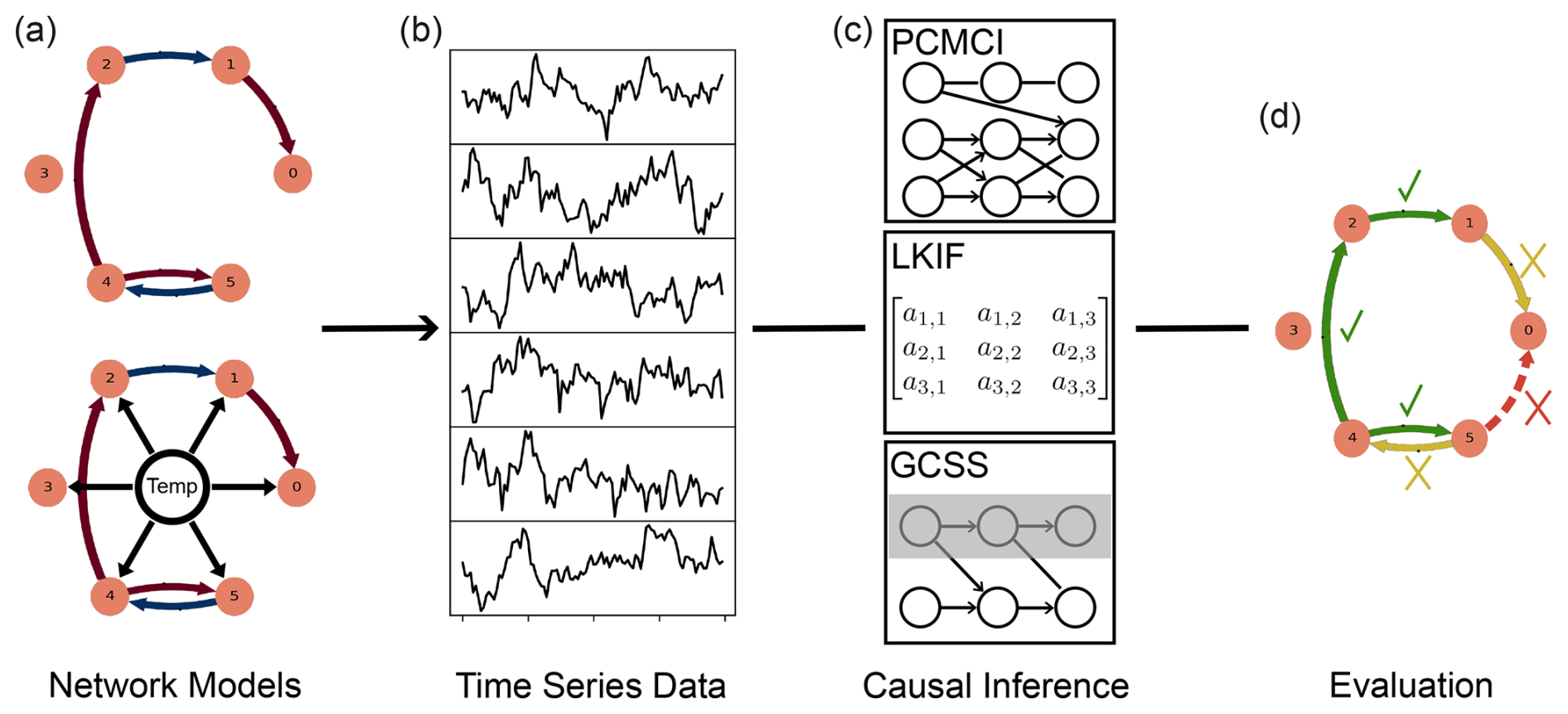
Figure 1 Conceptual overview of the methodological approach. (a) A network of interacting nonlinear dynamic systems generates (b) time series data for each variable. (c) Three causal methods are applied to the data to detect interactions, (d) their results are then checked against the ground truth network for accuracy evaluation. The chosen visualizations of methods in (c) are abstractions of their underlying modeling approach. In (d), green arrows indicate true positives, yellow arrows indicate false negatives, the red arrow indicates a false positive.

2.1 Data

Synthetic data are generated from a set of cubic stochastic differential equations (SDEs) each of which can exhibit a fold bifurcation, i.e., a tipping process once a certain threshold is crossed. More specifically, the cubic form is commonly used for an abstract system with hysteresis between two distinct equilibria (Wunderling et al., 2021; Bdolach et al., 2025). Each variable x_i evolves over time t as:

$$\begin{array}{}\text{(1)}& \begin{array}{rl}{\displaystyle }\dot{x_i}\left(t\right)=& {\displaystyle }-x_i(t{)}^{\mathrm{3}}+x_i(t)+c(t)\\ {\displaystyle }& {\displaystyle }+\sum _{j\ne i}{s}_{j,i}\left(x_j\right(t-\mathit{\tau })-\mathrm{1})+\mathit{\sigma }d{W}_i.\end{array}\end{array}$$

Nonlinearity is imposed on the dynamics of the variable itself through the cubic term $-x_i^{\mathrm{3}}$, with hysteresis due to the positive sign of x_i(t). The term ${\sum }_{j\ne i}{s}_{j,i}\left(x_j\right(t-\mathit{\tau })-\mathrm{1})$ introduces linear interactions between variables at a coupling strength s_j,i. Interactions may be delayed by a fixed τ (which is zero by default), resulting in a delayed differential equation (DDE). The Wiener noise dW_i is generated separately for each variable and scaled by σ. The variable c introduces time-dependent external forcing, in models of climate tipping elements this may resemble climate forcing. As c equally influences all state variables x_i, it can be referred to as a confounder. In the following experiments, c(t)=0 unless specified otherwise. At t=0, each variable is initialized to the stable equilibrium at x_i=1, with the other equilibrium at $x_i=-\mathrm{1}$. Once the sum of c, all interactions and noise crosses the threshold of $-\sqrt{\frac{\mathrm{4}}{\mathrm{27}}}$, only the negative stable equilibrium remains and the tipping process into this state starts (Klose et al., 2020).

The interactions between cubic models are conceptualized as the edges in a graph network model, with the cubic SDEs as nodes, see Fig. 1a. We manually designed networks of different sizes and densities, where a dense system has a higher connectivity of nodes, with a focus on feedback loops. We also chose the signs of interactions (i.e., negative or positive interactions) such that the resulting systems are stable under all parameterizations used in the following experiments. The manually designed systems can be found in Fig. A1, from which we derived systems of other sizes, see Appendix A.

2.2 Causal Inference Methods

We present three commonly used causal inference methods, namely the PCMCI, the LKIF and the GCSS methods, each with a different underlying concept of causality. We selected these methods as they share several compelling properties detailed in the following. Their performance converges at sample sizes we deem realistic for real-world applications and they are established in the literature. All methods can handle multivariate systems, either through fitting of vectorized models or through the inclusion of confounder variables in otherwise bivariate statistical tests. Every method also implements time-lagged causality detection by extending the dimensionality and therefore requires a maximal time delay at which interactions should be detected. For our analysis, the main task of the utilized methods is the identification of significant causal links from time series, this task is also referred to as causal discovery. All methods provide statistical significance tests at some confidence level α, indicating the error rate. Although the estimation of causal effect strengths is highly relevant to the interpretation of results, the different concepts of causality employed by these methods do not allow for a quantitative comparison of the accuracy of the strength estimations. In Appendix B, we provide a mathematical derivation and explanation of how these methods can be fitted to the data generated from the nonlinear dynamic systems of Eq. (1).

2.2.1 Peter–Clark Momentary Conditional Independence (PCMCI)

The PCMCI algorithm was introduced by Runge et al. (2019b) and combines the Peter–Clark (PC) algorithm with a momentary conditional independence (MCI) test. It has been successfully applied to various areas of climate science, including tipping points (Högner et al., 2025), atmospheric (Di Capua et al., 2024), oceanic (Falkena et al., 2025), cryosphere (Kromer and Trusel, 2023) and atmosphere–ocean interactions (Docquier et al., 2024).

In the PC phase of the algorithm, conditional independence tests are applied iteratively between a variable and past time steps of other variables, conditioned on an iteratively growing set of the most significant causal parents of the target variable. Once each variable has reached a stable set of causal parents, the MCI phase conducts final tests conditioned on the causal parents of both variables involved in a hypothesized causal link. Although the conditional independence tests appear to be pairwise in the strict sense, they provide multivariate analysis through the iterative changes to conditional variables: The method starts from a fully connected graph of interactions (between all variables, each at all analyzed time shifts), and then prunes false positives in the PC phase. The network is therefore optimized only by the iterative selection of conditional variables. On the other hand, the pairwise tests allow for a granular treatment of variables:

• Known causal connections can be imposed, or interactions can be prohibited if they are considered unrealistic or impossible.

• Sections of the data can be left out (masking), e.g., for missing samples or restriction to certain time periods.

• Masking can be applied exclusively when a variable is tested as a causal parent (or causal child, or conditional variable).

In this work, we utilize the PCMCI+ version of the algorithm, an extension that includes contemporaneous links (Runge, 2020). The underlying conditional independence test can also be chosen according to domain knowledge. In this study, we analyze the linear partial correlation test as it is the least computationally intensive, but nonlinear or model-agnostic tests are also available for usage with PCMCI (Runge, 2020), a comparison to other independence tests can be found in Appendix D. The significance level is applied to every independence test throughout the iterative phase and only provides an orientation about the significance of the final result, rather than an exact estimate of the error rate.

2.2.2 Liang–Kleeman Information Flow (LKIF)

The Liang–Kleeman Information Flow (LKIF) has only been applied to climate research very recently, with application to the cryosphere (Docquier et al., 2022) and land–atmosphere interactions (Zhou et al., 2024; Shao et al., 2024). A comparative study by Docquier et al. (2024) found similar reliability of PCMCI and LKIF under idealized settings. The LKIF method takes an information-theoretic approach to causality, by which the contribution of entropy from one variable to another constitutes its causal effect (Liang, 2021).

In practice, a low complexity model is fitted to the time series data. From this model, the entropy contribution is derived in the style of an intervention experiment, i.e., it is measured how the entropy of variables would change if one variable was missing from the model. The LKIF method is implemented with a linear SDE model, from which entropy transfers can be derived analytically (Liang, 2021).

$$\begin{array}{}\text{(2)}& \dot{\mathit{X}}=\mathbf{A}\mathit{X}+\mathit{b}+\mathit{\sigma }d\mathit{W}\end{array}$$

with X as the state vector, b a constant offset vector, σdW the increments of a vector of Wiener processes, and the coupling matrix A, which informs the causal structure of the process. While information flow analysis could also be applied to other structures of SDEs, such a derivation and implementation lies beyond the scope of this work.

Time lag analysis is implemented by extending the analyzed set of variables with time-shifted versions of the existing variables, up to some maximum time lag. Thus, the information flow from a time-lagged variable to the present state of other variables can be determined with the existing approach. For a causal link to be considered as detected in our evaluation it is sufficient to be statistically significant at any time lag.

2.2.3 Granger Causality for State Space Models (GCSS)

The Granger Causality for State Space Models (GCSS) method has so far seen little recognition in climate research, instead it has been widely used in the analysis of neural dynamics (Binns et al., 2025; Yue et al., 2025; Barnett and Seth, 2016). Granger Causality (GC) states that a variable is causal to another if its existence helps to predict the affected variable. Like for LKIF, the measurement of GC can be thought of as an intervention experiment, where one variable is removed and other variables are predicted less accurately because of it.

Barnett and Seth apply GC to a state space model (Barnett and Seth, 2015), which consists of an observation and a hidden process. It is time-discrete and able to describe vector-autoregressive processes with moving average components, i.e., a direct effect of past noise on current time steps. The state space model is fitted to the data using Canonical Correlations Analysis.

$$\begin{array}{}\text{(3)}& \begin{array}{rl}{\mathit{x}}_{t+\mathrm{1}}& =\mathbf{A}{\mathit{x}}_t+{\mathit{u}}_t\text{Hidden State Transition}\\ {\mathit{y}}_t& =\mathbf{C}{\mathit{x}}_t+{\mathit{v}}_t\text{Observation}\end{array}\end{array}$$

The vector of latent space variables x develops in discrete time steps t independently of the observations, while the vector of observation variables y is determined by the latent space variables and noise. The transition matrix A determines the causal structure of the latent process, which is then projected to the observation space by C. Variables u_t, v_t describe white process and observation noise.

While the chosen GCSS implementation does not provide information on the time distribution of causal effects, its hidden state dimension allows for an implicit time shifted analysis: The model can keep track of older values of some variable x_i,t by fitting a variable to behave as $x_{j,t+\mathrm{1}}=x_{i,t}$, thereby giving access to the value of x_i,t at one time step later and so on. If the maximal time lag of interactions is known, the maximal hidden state dimension can be determined accordingly. We implement a χ²-test for significance as suggested by the authors (Barnett and Seth, 2016, 2019), and scale its degrees of freedom with the dimension of input data (i.e., variable count).

2.3 Metrics

For easy comparison, we use a single metric that contains information on true and false positives (TP/FP) and true and false negatives (TN/FN). The Matthews Correlation Coefficient (MCC) is considered a good candidate for such a combined metric in comparison to other frequently used metrics and is equal to the phi coefficient in binary classification (Chicco and Jurman, 2020) and is thus related to the χ²-statistic as $\text{MCC}=\sqrt{\frac{{\mathit{\chi }}^{\mathrm{2}}}{n}}$(Everitt and Skrondal, 2010). The inclusion of all four basic metrics (TP, FP, TN, FN) avoids biases towards denser or less dense systems: In a network with a sparser graph matrix, the absolute number of false positives would likely increase (assuming a constant false positive rate), but other popular metrics like the F1 score do not include true negatives, while the MCC rewards true positives and true negatives symmetrically. The MCC is defined using the abbreviations for the basic metrics above:

$$\begin{array}{}\text{(4)}& \mathrm{\text{MCC}}={\displaystyle \frac{\text{TP}\cdot \text{TN}-\text{FP}\cdot \text{FN}}{\sqrt{(\text{TP}+\text{FP})\cdot (\text{TP}+\text{FN})\cdot (\text{TN}+\text{FP})\cdot (\text{TN}+\text{FN})}}}.\end{array}$$

An MCC score of one indicates perfect predictions, while a score of zero indicates no predictive power of the method (i.e., as good as random choices of positives and negatives), and minus one is the lowest score for predictions exactly opposite to the ground truth.

For more detailed analysis, we also provide true and false positive rates, which are calculated as follows:

$$\begin{array}{}\text{(5)}& \begin{array}{rl}\text{TPR}& ={\displaystyle \frac{\text{TP}}{\text{TP}+\text{FN}}}\\ \text{FPR}& ={\displaystyle \frac{\text{FP}}{\text{FP}+\text{TN}}}.\end{array}\end{array}$$

3 Results

For the following experiments, we use a default configuration of data and method parameters that we deem realistic for a setting in the analysis of climate tipping elements, and physical systems more broadly. We first vary several core parameters of the data generation, namely the number of provided samples, the coupling strength and the interaction delays, all of which may vary in applications to observational data. We further vary the network structure in terms of density, the number of variables and the inclusion of a global confounder variable, which may increase the complexity for the involved methods. Where a parameter is not varied explicitly, it is fixed to its default value listed in Table C1 in Appendix C. For each parameter varied in an experiment, its range is given as well. The default model network contains six variables with a low density of interactions, as visualized in Fig. A1c. One variable does not interact at all, the remaining variables are connected through five causal links. The network does not show tipping dynamics unless specified in the following experiments. Every experiment is run 100 times and we determine our metrics for each run, then show the average and standard deviation of those scores.

Supplementary results on different conditional independence tests for PCMCI are provided in Appendix D, a comparison of runtimes of the causal methods is found in Appendix E. Sensitivity tests to noise scale, sampling time steps and detailed network layout are provided in Appendix G.

3.1 Results for Data Parameters

Figure 2a shows a sharp rise in accuracy between 100 and 1000 provided samples for all methods, with LKIF being more reliable than the other two methods in this order of magnitude of available samples. For larger numbers of samples, the GCSS method yields nearly perfect prediction scores, while LKIF and PCMCI remain at MCCs around 0.8 and 0.6, respectively.

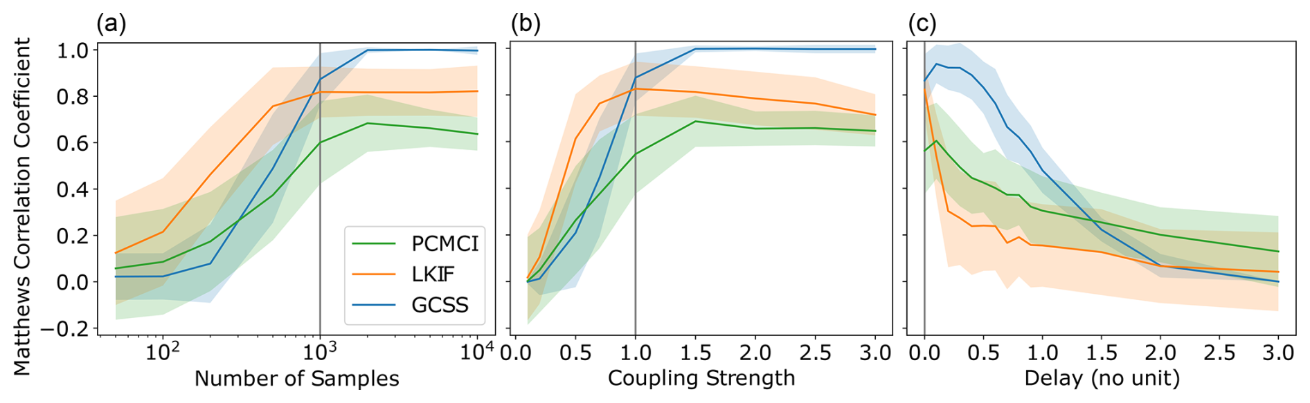
Figure 2 Relationship between prediction scores of the algorithms and basic data parameters: (a) number of samples, (b) coupling strength and (c) delay length (default: 1000 samples, coupling strength 1, no delay). Grey vertical lines indicate default values. Shaded areas indicate one standard deviation.

The scores for varying coupling strengths between the variables develop in a similar way (Fig. 2b): At low coupling strengths between 0.5 and 1, the LKIF method shows the best performance of the three methods, for higher coupling strengths the GCSS method predicts interactions perfectly again, both PCMCI and LKIF remain with imperfect scores for any coupling strength. While these results may appear abstract due to the lack of a dimension unit of the coupling strength, its magnitude can be illustrated with its impact on signals: The sampling rate of 10 samples per time unit means that the time-discrete approximation of the system (Eq. B2) results in a linear interaction coefficient that is ten times smaller, i.e., for a coupling strength of 0.5, the linear interaction coefficient is 0.05. Given the identical noise scale of all variables, a coupling strength of 0.5 would therefore imply a signal-to-noise ratio of $\frac{\mathrm{1}}{\mathrm{20}}$ for the detection of this causal interaction.

The results in Fig. 2a and b demonstrate the tradeoff made by the GCSS method, which comes with a moderately higher data intensity (and lower tolerance for ambiguity, w.r.t. coupling strength), but achieves nearly perfect results under ideal circumstances. The strict model assumptions for LKIF can explain its early convergence at high but imperfect accuracy, i.e., very few parameters need to be fitted (which leads to good results with few samples), but they lack explanatory power to capture the data entirely, no matter how many samples are provided.

When a delay is applied to all interactions (see Eq. 1), performance drops rapidly for the LKIF algorithm even at a delay of 0.1 time units, i.e., one sample, see Fig. 2c. The PCMCI algorithm experiences a gradual decrease in prediction accuracy. The GCSS method can handle small delays very well, and only becomes less reliable from a delay of five samples onwards. These qualitative differences can be explained by the underlying assumptions: The LKIF model derives time-lagged causality from a shift of input time series, which can only account for unidirectional time shifts, but not delayed feedback loops. The time-discrete methods of PCMCI and GCSS perform better for time lags. We consider it likely that GCSS provides higher explanatory power due to its state space model. The additional abstraction of a latent process effectively provides noise filtering and flexible time lag handling, which also comes at higher data intensity to achieve the scores seen in Fig. 2c.

3.2 Results for Network Configurations

Figure 3 shows results for the different networks of variables separately for each method. The corresponding manually designed systems can be found in Fig. A1 and vary in the number of variables and the density of edges in the graph, i.e., the number of interactions relative to the number of nodes. The GCSS method shows a large decrease in performance for larger networks, irrespective of the density. GCSS consistently shows slightly higher detection capabilities for networks of low density (see Fig. 3c). LKIF and PCMCI only show a slight decreasing trend in prediction scores for higher numbers of variables. LKIF detects networks of high density more accurately (see Fig. 3b), while PCMCI is ambiguous in this regard, as it scores better on networks of low density than of high density for small numbers of variables, but high density networks seem to converge at slightly higher scores for higher numbers of variables (see Fig. 3a).

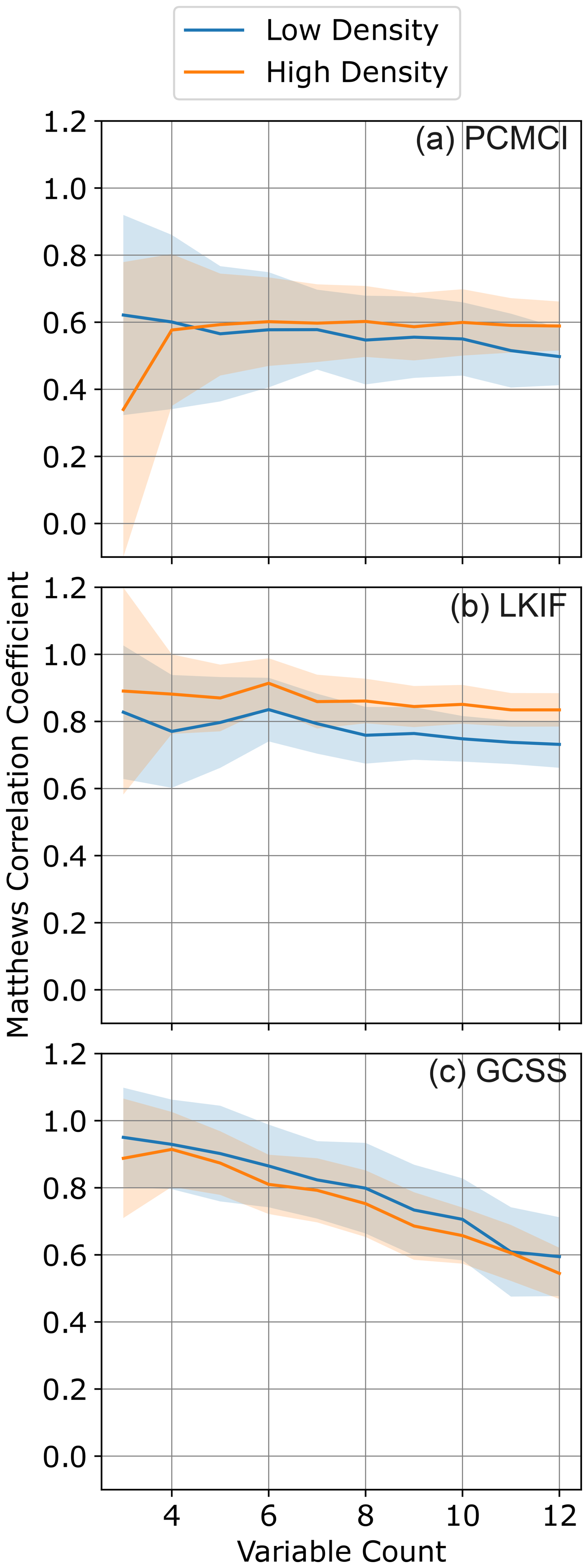
Figure 3 Prediction capabilities of the (a) PCMCI, (b) LKIF, and (c) GCSS methods for varying number of variables and interactions in the underlying model system.

In these and other tests, we observed that the optimal choice of a significance level α for any method depends heavily on the given network size and density as well as on other data parameter choices. Therefore, using a different α than in the experiment may yield a qualitatively different accuracy landscape. However, our choice of α=0.05 is based on its common choice in the literature to ensure reasonable confidence.

3.3 Results on External Forcing

In the final experiment, we apply an external forcing to all variables, driving them closer to a tipping point. When this forcing variable is not included in the causal analysis, the forcing effects may wrongfully show up as an interaction between other variables. The forcing parameter c in Eq. (1) is time-dependent (with t≥0), rising linearly for 50 units of time, and staying constant for the remaining 50 units of time at some maximum value c_lim. At the highest forcing strength f, given on the x axis of Fig. 4, this maximum value matches the bifurcation point of the cubic equation without interactions and noise, so that tipping is enforced. The fast dynamics of the system ensure that no rate-induced tipping occurs.

$$\begin{array}{}\text{(6)}& c\left(t\right)=\left\{\begin{array}{ll}\frac{c_{\text{lim}}}{\mathrm{50}}\cdot t& \text{if }t<\mathrm{50}\\ c_{\text{lim}}& \text{else}\end{array}\right.,c_{\text{lim}}=-\sqrt{{\displaystyle \frac{\mathrm{4}}{\mathrm{27}}}}\cdot f\end{array}$$

The forcing parameter c could resemble the impact of global warming on climate tipping elements. This variable is also referred to as a confounder, as it influences all time series without necessarily being part of the causal analysis. We then compare the detection scores between the exclusion and inclusion of the confounder in the causal analysis.

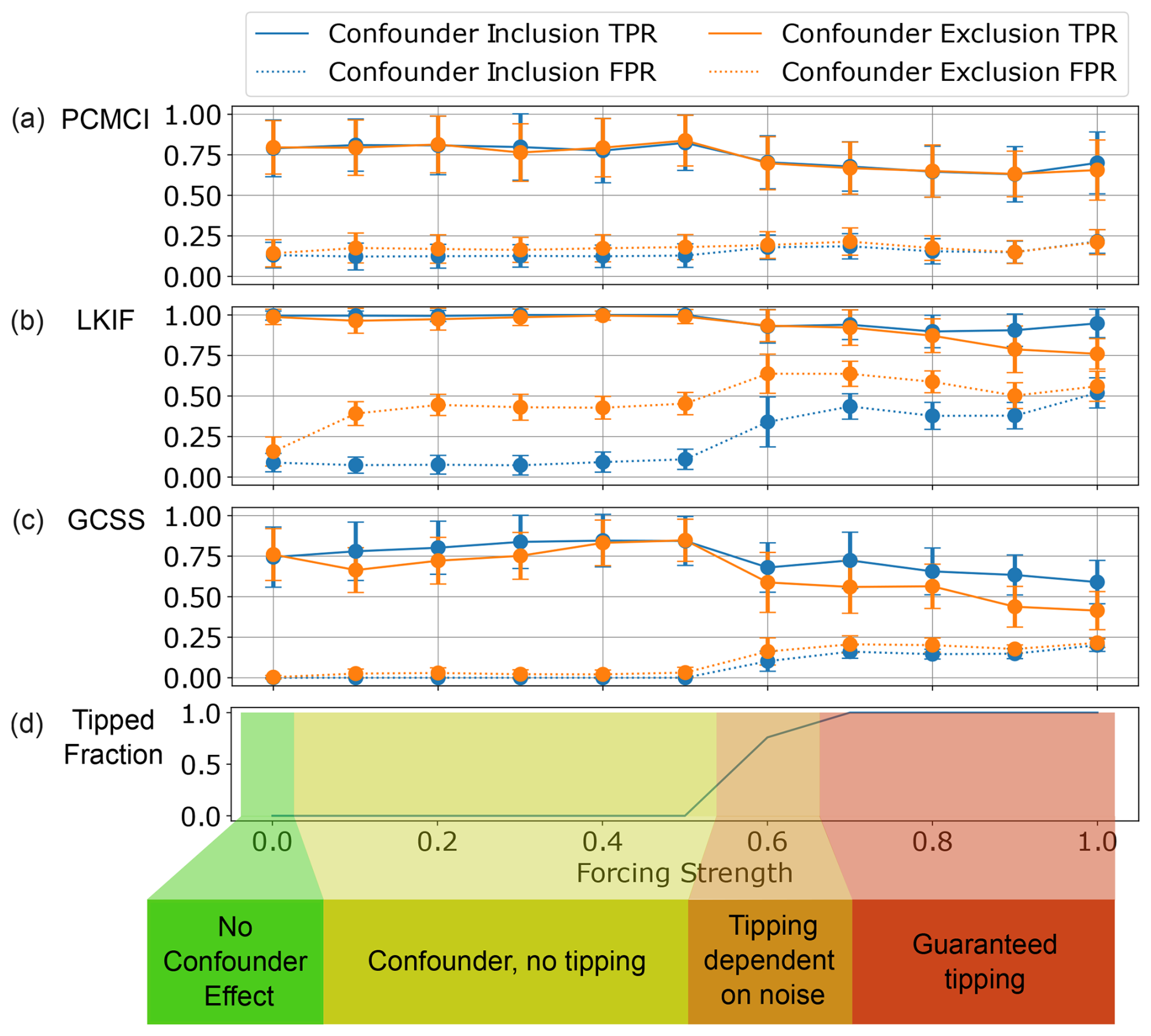
Figure 4 The influence of confounders on the detection of tipping point interactions. (a–c) Prediction capabilities under increasing confounder strength, with true and false positive rates for causal analysis including and excluding the confounder variable, respectively. Vertical lines indicate one standard deviation. (d) Fraction of time series that show tipping processes, as noise plays a larger role around the threshold. Shading indicates the color-coded confounding scenario.

As shown in Fig. 4, when the confounder is excluded from analysis and weak forcing is applied (i.e., below any tipping points), the false positive rate of the LKIF algorithm rises by more than one standard deviation in comparison to the absence of forcing. However, when the forcing variable is included in the causal analysis, the introduction of weak forcing does not have a significant influence on the false positive rate of LKIF. Similarly, the true positive rate of GCSS drops upon introduction of forcing for an excluded confounder, but remains unchanged if the confounder is included in the causal analysis. Notably, the PCMCI method does not show any clear trends from the inclusion of a forcing variable.

When a tipping point is crossed (forcing strength ≥0.6, right hand side in Fig. 4), one or more variables undergo abrupt tipping processes into their alternative stable states. Due to the interactions between tipping elements in this model, the forcing strength required to tip at least one element is lower than for an isolated element (which would tip at a forcing level of 1). In Eq. (1), the previous equilibrium around x=1 ceases to exist as the function values become strictly negative for any x>0 due to the strong effect of c(t).

All methods show a significant decrease in true positives when tipping events are present in the data. For LKIF and GCSS, we also detect a rise in false positives. Regardless of the inclusion of the confounder, a false positive rate >25 % for LKIF sheds doubt on any results under such a setting. Especially in applications to physical systems, which are expected to have relatively sparse causal interactions, a false positive rate of 25 % may produce more false positives than true positives in absolute terms. For GCSS and PCMCI, the low rate of true positives also would make it difficult to draw robust conclusions from an experiment under such conditions. While PCMCI is the least affected by confounding and it can compete with the other methods in scenarios with tipping events, its baseline performance still limits the confidence in its results in all presented scenarios.

4 Discussion

In general, our results on the relationship of sample count and detection capabilities are encouraging for the usage of these methods, even under settings with limited data availability, e.g., around 500 samples (Fig. 2a). Similarly, one can expect to reliably detect causal relationships with a coupling strength of 0.7 or more using the LKIF method (Fig. 2b). Notably, the GCSS method is a very reliable choice for settings with either large sample counts or strong causal interactions, which could make it more interesting for e.g., analysis of time series from long runs of climate models. The MCC scores achieved in these synthetic cases reveal clear trends, but may overestimate the performance in applied experiments due to the idealized identical timescales of all involved systems and our choice of default parameters close to the convergence conditions of all methods.

In the following, we derive two recommendations on data selection (1a, b), and one on the choice of a causal method (2). The results on interaction delays (Fig. 2c) call attention to the importance of time scales in the application to physical systems. Every physical interaction of tipping elements operates at some time delay, simply in order to transfer information through various means (e.g., transport of heat, pressure, precipitation, salinity, etc.). Given our presented results on the influence of time delays on detection capabilities, we give the following recommendation:

Recommendation 1a: The sampling rate of observations should match the scale of time delays of interactions. The chosen sampling rate should also not be multiple orders of magnitude smaller than the internal timescale of the involved systems, see Appendix G.

A possible explanation for the large performance drop of LKIF under delays is its strict assumption of an underlying SDE, i.e., a time-delayed effect (representable by a DDE) cannot be reproduced inside the model. Even though the input time series are shifted in time for time-lag analysis, such shifts cannot reproduce delays in feedback loops. The good detection capability of GCSS is likely caused by its larger model complexity. It explicitly allows for the representation of delayed variables, and computes the significance of a variable's causal effects across all time lags.

The assumption of stationarity is crucial to the linearization of the chosen dynamical system, as described in Appendix B. In the analysis of climate tipping points, one has to assume a violation of the stationarity assumption given that the expected levels of warming in the next decades could be sufficient to cross multiple tipping points (Armstrong McKay et al., 2022).

Recommendation 1b: In the presence of a destabilizing forcing variable, the inclusion of this forcing variable in causal analysis is strongly recommended. Even for a nonlinear system response to forcing, this inclusion mitigates any negative effects of forcing on prediction capabilities, as long as the analyzed dynamic systems do not enter a tipping process (Fig. 4). The inclusion of the confounder is less crucial to the performance of the PCMCI and GCSS methods than to the LKIF method. We do not recommend any of the discussed causal methods if a tipping process is present in analyzed data, assuming similar other parameters in terms of network size, sample count and coupling strength.

Throughout the experiments, the different methods showed respective strengths and weaknesses. We summarize them here in order to give advice on the choice of a causal method in a concise manner.

Recommendation 2: The choice of a causal method fitting to the known conditions is crucial for successful causal analysis. Two methods have concrete niches for their application: The GCSS method is advisable to be used if one can assume significantly delayed causal effects, and for settings with large sample counts, few variables and/or strong interactions. The PCMCI method offers the largest flexibility and should be used when domain knowledge needs to be integrated into causal analysis, e.g., prohibiting impossible links or masking data. The LKIF method offers the best performance in most cases that do not fall under any of the above constraints. Note that the usage of multiple of the presented methods can serve as a robustness test under conditions that do not fall clearly into any category.

Previous assessments of PCMCI (with the partial correlation test) confirmed its weaknesses in nonlinear settings (Delforge et al., 2022; Liang et al., 2025). Our results also highlight a significant difference between the performance of PCMCI and LKIF in most parameter settings, which extends a previous comparison study by Docquier et al. (2024), which found a more similar performance of the two methods in linear systems and for larger numbers of samples. Our results confirm the difficulties with time lags for the LKIF method identified in the former study. The existing literature provides ambiguous results on the connection between the number of samples and prediction performance, with some studies showing a relatively small increase in prediction scores for growing sample size (Assaad et al., 2022), others show trends that are similar to our results, but often with better scores at low numbers of samples (Runge, 2020; Liang et al., 2025). We consider it likely that this difference is due to the choice of linear, time-discrete models and larger interaction coefficients in these studies.

5 Application to Climate Tipping Points

We demonstrate the application of causal inference methods to climate tipping points on the interactions between the AMOC and Arctic summer sea ice (ASSI). We apply PCMCI and LKIF, as both can restrict analysis to seasonal sections of time series. Data masking is not possible with GCSS in a straightforward way as the method fits its state space model to the entire time series at once, so gaps or masked segments would require multiple model fits. Even though ASSI is not considered a tipping element of the climate system (Lenton et al., 2025), abrupt shifts in ASSI have been detected in recent studies on CMIP6 models (Terpstra et al., 2025; Angevaare and Drijfhout, 2025), indicating at least a nonlinear relationship between forcing levels and sea ice coverage. The ASSI extent has decreased drastically due to global warming over the past decades, and an ice-free Arctic in summer is projected to occur by 2050 (Jahn et al., 2024).

The current literature is mostly based on model experiments and suggests a stabilizing effect of a weakening AMOC on Arctic sea ice on annual to decadal timescales due to the reduced northward heat transport of the AMOC (Mahajan et al., 2011; Docquier and Koenigk, 2021; Weijer et al., 2022). The effect of Arctic sea ice decline on the AMOC is subject to multiple, partly competing explanations: The increasing amount of freshwater from sea ice melt is considered to have a destabilizing effect on the AMOC (Li et al., 2021; Liu and Fedorov, 2022; van Westen et al., 2024a). On the other hand, the larger area of exposed sea surface may lead to an increase in heat loss (Wu et al., 2021) and therefore a stronger convection in the winter, or an increase in radiative warming (Sévellec et al., 2017; Jenkins and Dai, 2022), which would weaken convection.

For our data–driven analysis, we use a sea surface temperature (SST) fingerprint of the AMOC established by Caesar et al. (2018) based on ERA5 data (Hersbach et al., 2023) as previously used in data-driven causal analysis by Högner et al. (2025), and reanalysis data of Arctic sea ice concentration (E.U. CMEMS, 2024b) based on the neXtSIM model (Williams et al., 2021). We aggregate the Arctic sea ice concentration over a 180° slice (90° W to 90° E), i.e., on the side facing the Atlantic, and we only include cells above the 66th percentile of variation of sea ice concentration, as these show the strongest interaction signal (e.g., the meltwater flux would be strongest from these cells), see Appendix F.

Arctic sea ice variability is largely driven by atmospheric temperatures in the Arctic (Olonscheck et al., 2019) and oceanic heat transport (Docquier et al., 2022). In turn, Arctic sea ice concentration plays a major role in the regional climate of the Arctic (Carvalho and Wang, 2020). A reduction in ASSI was found to explain temperature increases especially in autumn and winter (Huo et al., 2025). To rule out a potential confounding effect of temperature conditions in the Arctic on both Arctic sea ice and the AMOC, we use an aggregate of sea surface temperature and ice surface temperature data of the Arctic Ocean (E.U. CMEMS, 2024a). All variables are detrended and we remove seasonal trends, i.e., for each sample point, the average value of its month is subtracted.

As mentioned, the most drastic effects of global warming on Arctic sea ice are observed in summer. Additionally, the described physical mechanism of meltwater influx from Arctic sea ice to the AMOC also warrants a focus on the summer season of Arctic sea ice. We therefore restrict analysis to the period from March to September, i.e., the months from the maximum to the minimum of Arctic sea ice extent (Stroeve and Notz, 2018). This is possible in PCMCI and LKIF by masking data, i.e., certain time periods of data are ignored in causal analysis. For the PCMCI method, we can further define these masks to be applied only to the causal parent, i.e., we search for causal effects originating in the summer months. Therefore our analysis may only detect interactions from ASSI to the AMOC, but may include effects of the AMOC on Arctic sea ice changes later in the year, depending on the estimated effect delay. For clarity, we consistently refer to this masked sea ice concentration as ASSI in the context of the causal analysis. The LKIF method simply drops all masked samples.

Given a relatively short observation period of 31 years, it is infeasible to conduct analysis on annual data. In order to still capture the inherent time scales of oceanic and cryospheric processes (following recommendation 1a), we decide on a monthly timescale. Our analysis therefore deals with a sample count of 217 samples for LKIF, while PCMCI may involve delays of up to 5 months (beyond the mask on the causal parent), resulting in the full 372 valid samples (in causal children and conditional variables). Following our results in Fig. 2a, we are sufficiently confident to draw consistent conclusions with additional robustness tests (see Fig. F1b–e), although a higher sample count would reduce uncertainty.

With the PCMCI method, our causal analysis reveals a bidirectional interaction between ASSI and the AMOC, see Fig. 5. The effect of the AMOC on ASSI is found to be stabilizing, i.e., a weakening of the AMOC would increase ASSI concentration. The ASSI concentration is found to have two effects on the AMOC at different time delays, the stronger one is a stabilizing effect on the AMOC with a delay of one month, i.e., a loss of ASSI would strengthen the AMOC after one month. Additionally, PCMCI shows a weaker and more delayed destabilizing link (time lag of five months, see arrow labels in Fig. 5). Extended experiments with other sea surface temperature datasets support the robustness of all detected links, with the exception of the five-month destabilizing link, see Appendix F. These links are considered stabilizing in the sense that the degradation of one element increases the tipping resilience of the other, affected element. However, the full circular interaction still implies a destabilizing loop (i.e., a weaker AMOC leads to more ASSI, which leads to an even weaker AMOC).

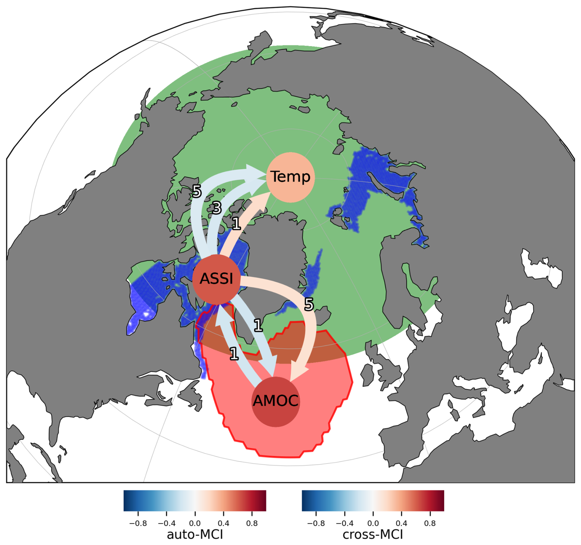
Figure 5 Causal network between ASSI (blue), the AMOC (red), and Arctic temperatures (green), as detected by the PCMCI method. A bidirectional stabilizing interaction of ASSI and the AMOC is found, while a confounding effect of Arctic temperatures is refuted. The arrow shading indicates the sign and significance derived by PCMCI. Note that the highest effect strength for the interaction from ASSI to the Arctic temperatures is found at a lag of three months, implying an inversely proportional effect.

The LKIF method (Fig. F1a) also shows a link from the AMOC to ASSI, implying an information transfer of 9.5 %. It does not detect any further causal links. However, we have several reasons to consider PCMCI the more reliable approach in this application example:

• LKIF considers a significantly lower amount of samples in its analysis.

• There are inherent delays in the underlying physical mechanisms, which may make PCMCI more reliable, see Fig. 2c.

• Such delays are further supported by the findings of PCMCI, with delays up to 5 months.

We therefore focus our further analysis on the results of the PCMCI method. With PCMCI, we find a causal effect from ASSI to the Arctic temperatures. Effects are found at delays of one, three and five months, of which the delay at three months is the strongest by a factor of five. This effect confirms the literature findings by which a decline in ASSI increases Arctic temperatures. Although the causal effect of temperatures on Arctic sea ice area, as detected in Docquier et al. (2022) in March and September, is not detected in this experiment, the integration of Arctic surface temperatures underlines that our detected effects occur between ASSI concentration and the AMOC rather than between sea and ice surface temperatures in the Arctic (as measured by the Arctic temperature variable) and the North Atlantic (as measured by the AMOC fingerprint).

With a causal strength estimation method (linear mediation, see Runge et al., 2015), we can estimate that the stabilizing effect from the AMOC to ASSI would result in an increase of 0.1 percent points in ASSI concentration for every 1 Sverdrup (Sv) of AMOC weakening. Given that model and observation estimates of the AMOC strength vary between 15 and 25 Sv (van Westen et al., 2025; Drijfhout et al., 2025; Frajka-Williams et al., 2019), this effect would be very weak even in the case of a shutdown of the AMOC.

In the other direction, the strength estimation for the stabilizing link from ASSI to the AMOC implies that for every ten percent points of ASSI concentration loss, the AMOC would be strengthened by 0.61 Sv one month later. The destabilizing link at five months delay would imply a weakening of the AMOC by 0.14 Sv for the same loss of ASSI. The contradictory direction of these links may be explained by the competing physical effects on different timescales: The freshwater influx destabilizing the AMOC may take several months due to the required oceanic transport, while increased heat loss of surface waters to the atmosphere is a more immediate effect of reduced sea ice concentration and may explain the stabilizing link found here.

In this applied example of two of the three tested algorithms, a data-driven analysis of interactions between ASSI and the AMOC on time scales of months, we find indications for all three interaction effects suggested in the literature:

• A weakening of the AMOC would stabilize ASSI due to a reduced northward heat transport (Mahajan et al., 2011; Docquier and Koenigk, 2021; Weijer et al., 2022). This effect is confirmed by PCMCI and LKIF.

• Loss of ASSI may stabilize the AMOC, as increasingly exposed ocean surfaces may lose more heat to the atmosphere (Wu et al., 2021).

• The freshwater influx from melting ASSI may destabilize the AMOC, although likely on larger timescales (Li et al., 2021; Liu and Fedorov, 2022; van Westen et al., 2024a). Model results are therefore in agreement with the high delay detected by the PCMCI method for this effect. The effect may also be explained by radiative warming of exposed ocean surface (Sévellec et al., 2017; Jenkins and Dai, 2022).

GCSS is not suited to be applied to this example, because it does not offer the option of systematically masking the data, and thus, wanting to understand seasonally constrained interactions, cannot be applied here. LKIF lacks several causal effects, as it struggles to detect delayed effects and implements masking in a way that drastically reduces available sample size. With PCMCI, delays and data masking do not affect detection power as much (Fig. 2c), and a stable causal network is detected. While our results on nonlinear synthetic data suggest intermediate reliability of PCMCI for the given number of samples (Fig. 2a), the literature suggests much better performance of PCMCI in linear systems (Docquier et al., 2024; Runge, 2020). Therefore, the weaker nonlinearity or even linearity of ASSI may explain the high robustness of our results and their agreement with physical effects described in the literature. A potential limitation of this study is the lack of a detected causal effect of Arctic temperatures on ASSI concentration as suggested in the literature (Olonscheck et al., 2019). This could be explained by the bidirectionality and short timescales involved, as indicated in sensitivity experiments (Fig. F3), and may offer an opportunity for future work, preferably with data series of smaller timesteps (e.g., weekly).

The strength estimation of effects derived from our causal analysis likely underestimates the magnitude of the interactions, mainly because much of them may happen on slower time scales, as suggested by model studies (Mahajan et al., 2011; Li et al., 2021; Liu and Fedorov, 2022), which we are not able to analyze due to limited data availability on longer time scales. The short delays on monthly time scales assessed here, can only capture relatively fast parts of the (assumed) physical interactions, leaving more delayed and more continuous interactions (e.g., the meltwater fluxes from different regions of the Arctic Ocean arriving in different months), as well as long-term responses out of the picture. The detected short-term impact of ASSI on the AMOC is thus an impact on sea surface temperatures, as measured by the AMOC fingerprints, which in turn drive convection strength mainly in winter and on larger timescales (Petit et al., 2020).

Furthermore, the impact of an AMOC weakening on oceanic heat transport appears to be nonlinear, i.e., while the current cold anomaly in the North Atlantic is largely constrained to the subpolar gyre region (Caesar et al., 2018), projections of an AMOC shutdown predict sea surface temperatures to drop massively across the Arctic and subpolar seas (van Westen et al., 2024b), which may well have a larger effect on Arctic sea ice than a linear extrapolation of current observations would imply.

In future analyses, the inclusion of larger time scales could add to the already observed effect strength, however, this would require using data from ESMs. For a detailed picture of the causal structure under AMOC weakening, this would require experiments that extend past 2100. Model data is generally an interesting future field to apply causal analysis to tipping processes and interactions.

6 Conclusions

All three causal inference methods analyzed in this paper can be reliable tools for the detection of interactions of climate tipping elements. However, we determined several conditions for sufficient reliability that need to be considered for their application. Researchers should take adequate care that sufficient sample sizes are available, while sampling on a time scale roughly matching expected interaction delays. Strong nonlinearities in data, e.g., from tipping processes, reduce the reliability of the methods significantly. The choice of a causal method is crucial and depends to a large degree on known conditions: The GCSS method appears most useful in large datasets with few variables, or if significant delay effects can be expected. The LKIF method is most reliable for application cases on the lower end of data availability and interaction strengths, while the PCMCI method shows weaker detection power across most parameterizations, but offers enhanced flexibility for the inclusion of expert knowledge.

Although this work covers several common challenges in real data, the behavior of physical systems remains more complex than the idealized models we analyzed. Such phenomena include processes on multiple time scales of systems and their interactions, or seasonality and regime dependence in data. Further research could identify approaches and recommendations on causal analysis in the presence of tipping events or how expert knowledge can be integrated into causal analysis to tackle the additional complexity of physical systems.

In an applied experiment, we utilized the PCMCI method to detect a bidirectional stabilizing interaction between the ASSI and the AMOC on reanalysis data. Despite constraints in terms of data availability, we find that these interactions resemble the physical effects suggested by domain experts and model experiments. Due to a lack of long-term observational data on Arctic sea ice, we consider it the most promising approach for further investigations to apply the presented causal methods to data from ESMs to explore the role of time scales and regime shifts under global warming on these interactions.

Overall, these results encourage the usage of causal inference methods for climate tipping elements under careful consideration of the data availability and assumptions on the observed processes.

Appendix A: Interaction Networks

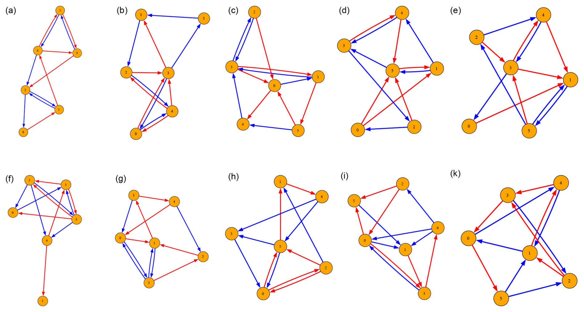
Figure A1 shows six network systems that were manually designed with a focus on stability in the absence of forcing (c=0 in Eq. 1). Networks of sizes between two shown sizes are derived by removing nodes from the next larger network, starting with the node with the highest index. The default network used in the experiments in this study is shown in panel c.

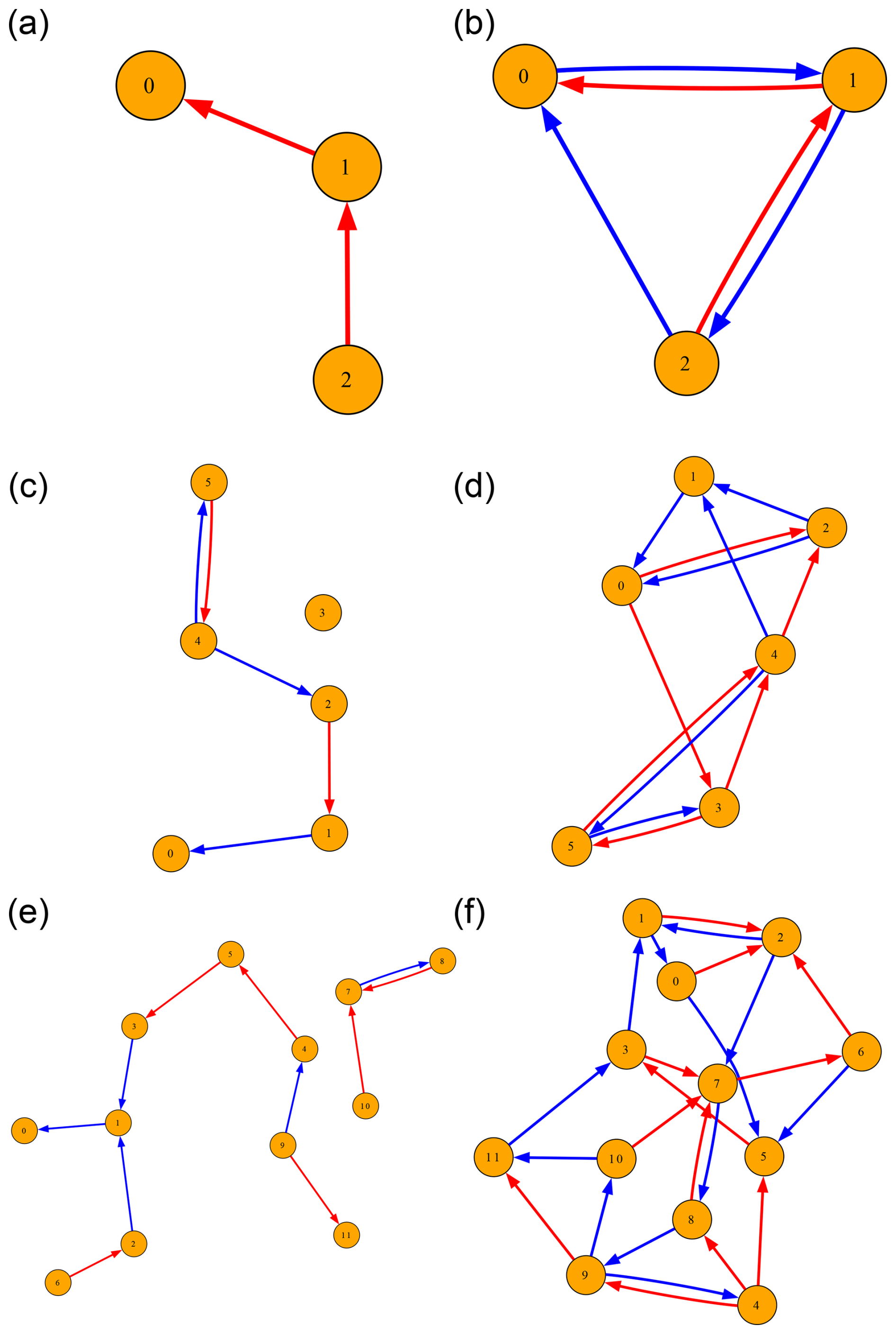
Figure A1 The different systems used for synthetic data generation, with varying numbers of variables and two density levels (where a, c, e are sparse systems, and b, d, f are dense). Red edges indicate positive interaction strength, blue edges indicate negative interaction strength.

Appendix B: Fitting Models to Data

Both the LKIF and the GCSS method are based on explicitly fitting a model to the input data, each of which assumes linearity in some form. As we use PCMCI with the partial correlation test, the method implicitly assumes a linear impact of interactions on variables, too. Therefore none of the models assumed by these methods fit exactly to the synthetic data generation model with a cubic differential equation. However, two additional assumptions about the data generation process can fix this issue.

• Firstly, if the system is stationary, i.e., no forcing is applied and the system is in equilibrium from the start, then the system can be approximated by a linearization around the equilibrium (i.e., a first-order Taylor expansion). Equation (1) in its linearized form around x=1 with c=0 and τ=0 thus becomes:

  $$\begin{array}{}\text{(B1)}& \dot{\mathrm{\Delta }{x}_i}=-\mathrm{2}\mathrm{\Delta }{x}_i+\sum _{j\ne i}{s}_{j,i}\mathrm{\Delta }{x}_j+\mathit{\sigma }d{W}_i,\end{array}$$

  where $\mathrm{\Delta }{x}_i=x_i-\mathrm{1}$ describes the deviation of a variable from its equilibrium. Note that this model aligns with the model employed by the LKIF algorithm. However, large noise may move the state out of the proximity of the equilibrium that is approximated well. Additionally, the interactions between variables technically violate the stationarity assumption (i.e., noise in one variable can move the equilibrium of another variable around which its linearization was conducted).

• Secondly, time discretization is required to numerically integrate the model. The GCSS method further explicitly assumes a time-discrete process for the underlying data. Any linear ordinary differential equation can be approximated by a time-discrete vector autoregressive process. We denote the derivation with the Euler–Maruyama scheme.

  $$\begin{array}{}\text{(B2)}& \begin{array}{rl}{\displaystyle }\mathrm{\Delta }{x}_{i,t+\mathrm{\Delta }t}=& {\displaystyle }\mathrm{\Delta }{x}_{i,t}+\mathrm{\Delta }t(-\mathrm{2}\mathrm{\Delta }{x}_{i,t}+\sum _{j\ne i}{s}_{j,i}\mathrm{\Delta }{x}_{j,t})\\ {\displaystyle }& {\displaystyle }+\mathit{\sigma }\mathrm{\Delta }{W}_{i,t},\end{array}\end{array}$$

  with $\mathrm{\Delta }{W}_{i,t}\sim \mathcal{N}(\mathrm{0},\mathrm{\Delta }t)$. With a suitable choice of Δt, this procedure can approximate the original process with arbitrary accuracy. This linear, time-discrete model transformation aligns with the model of GCSS, and fulfills the model assumptions of PCMCI. Since there is an inherent delay effect between the values of a causal parent and a causal child in a linear differential equation, we choose Δt=0.1 for our experiments as a tradeoff between accuracy and this implicit delay length.

Appendix C: Parameterization of Synthetic Data Generation

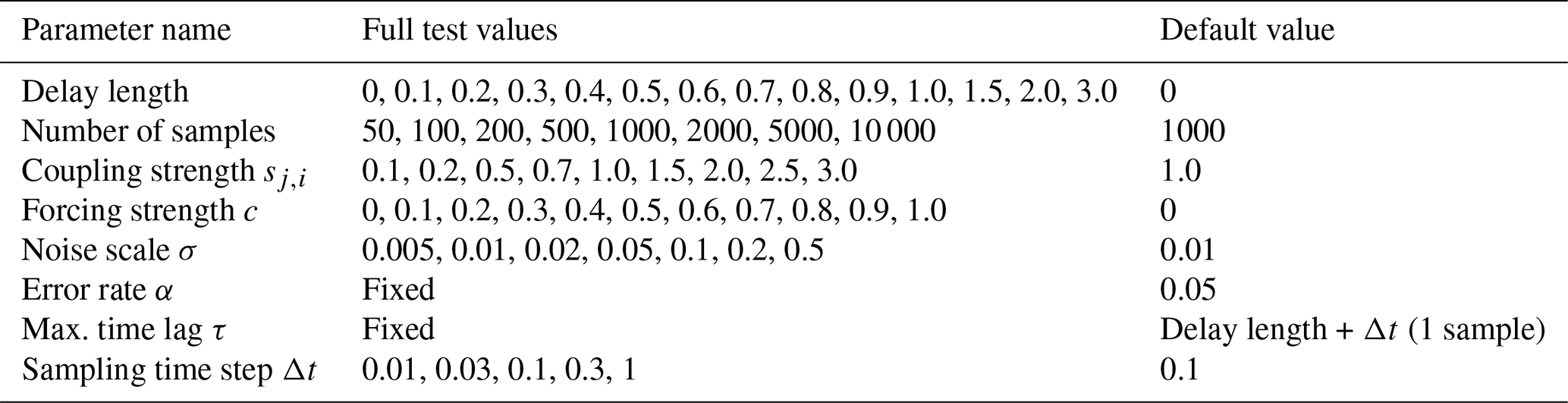
Table C1 lists the parameters of the synthetic data generation and of the causal inference methods (error rate and max. time lag) in their full ranges for the corresponding experiments and their default values where they are not varied explicitly.

Table C1 Parameters used in the experiments with their corresponding ranges.

Appendix D: Conditional Independence Tests in PCMCI

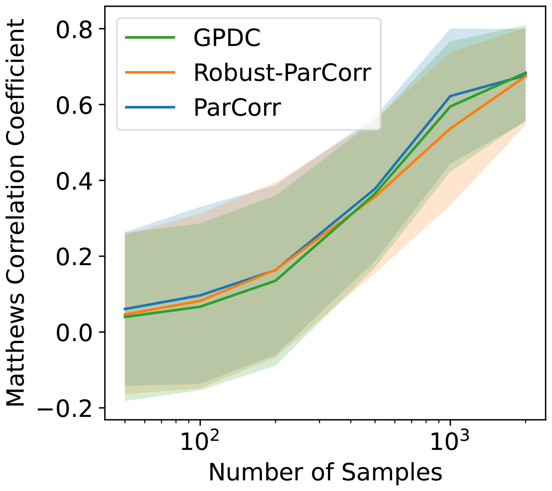
As the PCMCI method provides several different conditional independence tests, Fig. D1 displays the results of the sampling experiment (from Fig. 2a) with the robust partial correlation test, which normalizes the distribution of samples to fulfill the assumptions of partial correlation tests more closely, and with the nonlinear Gaussian process distance correlation (GPDC) test (Runge et al., 2019b). As the GPDC test is significantly more computationally intensive, we only conduct this experiment with up to 2000 samples.

The differences in detection scores between the analyzed conditional independence tests is very small and lies within half a standard deviation, with the partial correlation test yielding a slightly higher MCC.

Figure D1 MCC scores of PCMCI with three different conditional independence tests.

Appendix E: Runtimes of Causal Methods

When applied to a small number of variables as in this study, all presented causal algorithms can be run on standalone hardware for singular executions. Here we present statistics of their runtime over 100 runs at the default settings of Table C1 on the PIK high performance computer system, using AMD EPYC 9554 Genoa processors at 3.1 GHz.

The GCSS algorithm performs with a very consistent runtime of about 10⁻² s, while the LKIF method shows large outliers with higher runtimes, but a median runtime even lower than that of GCSS. PCMCI (with the partial correlation test) is the slowest algorithm and takes more than 0.1 s per run.

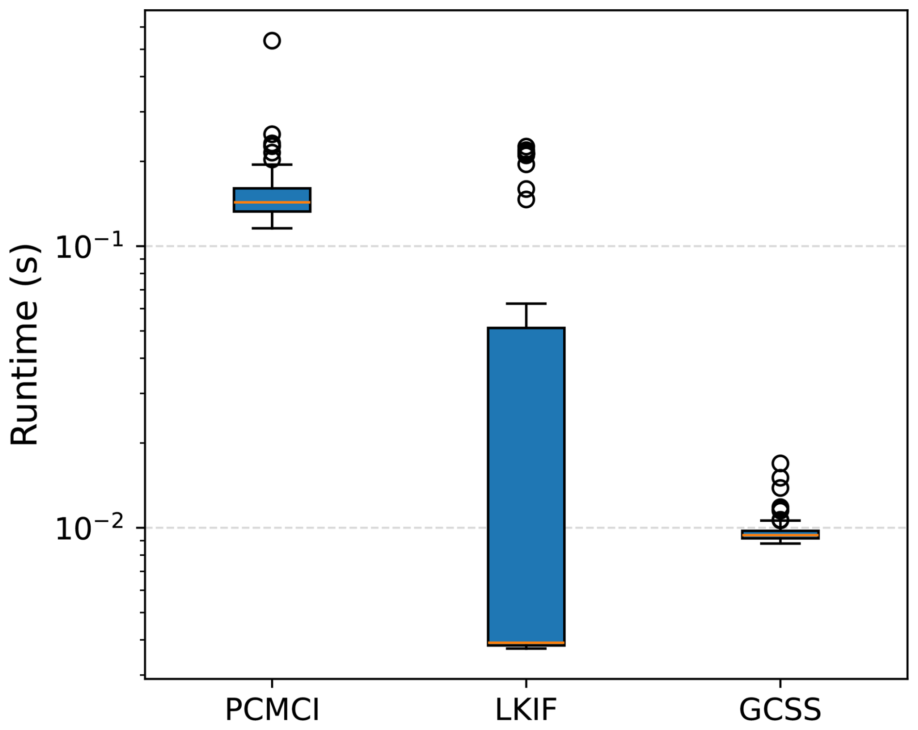
Figure E1 The runtime statistics of the presented causal methods. The orange line indicates the median, the blue bar mark values between the 25th and 75th percentile, and whiskers extend to the outermost data point that is within 1.5 times the interquartile range (i.e., the size of the blue bar). Outliers beyond the whiskers are represented by circles.

Appendix F: Extended Experiments on ASSI and AMOC

We conduct further experiments to test the robustness of the detected interactions between ASSI and the AMOC. Firstly, the LKIF method is applied, and confirms only the link from the AMOC to ASSI, see Fig. F1a. Secondly, several alternative data sources for sea surface temperatures are used to determine the AMOC fingerprint as established by Caesar et al. (2018): Data from HadCRUT5 (Morice et al., 2021), HadISST4 (Kennedy et al., 2019), COBE-SST2 (Hirahara et al., 2014) and ERSSTv5 (Huang et al., 2017) are aggregated and preprocessed in the same manner as the ERA5 data in the main part of this study. These datasets were prepared in Högner et al. (2025) and are used here unchanged. While the HadCRUT5, HadISST4 and ERSSTv5 datasets are related through their usage of partly identical raw datasets (Morice et al., 2021), ERA5 and COBE-SST2 data are fully independent of those (Thorne et al., 2026). The causal analysis shows highly similar results for all but the HadCRUT5 data set, see Fig. F1b–e. While the slower and weaker destabilizing link from ASSI to the AMOC is not confirmed by these robustness tests, they provide strong evidence that the main mechanisms identified in our experiment are robust to observational noise and differences in reanalysis procedures.

In the discussion of the experiment, we refute the hypothesis that the Arctic temperatures have a confounding effect on the AMOC and ASSI. Here, we test the robustness of the interaction between the remaining two variables. When the Arctic temperatures are left out of the causal analysis, interactions between the AMOC and ASSI remain identical in signs and strength, see Fig. F2.

We further test the robustness to different aggregations of ASSI concentration. In the main experiment, we set a threshold at the 66th percentile to integrate several important sites of Arctic sea ice formation and flux. Figure F3 shows results of causal analysis without such a filter, and cutting off at the 50th, 75th and 90th percentile. We can observe that the destabilizing impact of the AMOC is found for all settings except for the unfiltered aggregation. The 50 % aggregation finds only the slow effect of sea ice on the AMOC, while the 75 % and 90 % experiments show only the fast effect. The signs of the effects are consistent across all configurations, and every effect described in the main experiment is found in at least two other configurations. A directed effect of Arctic temperatures on ASSI is not detected in any configurations, although the unfiltered results find an ambiguous contemporaneous interaction. We conclude that the chosen 66th percentile boundary appears as a good tradeoff, where all three signals are clearly identifiable.

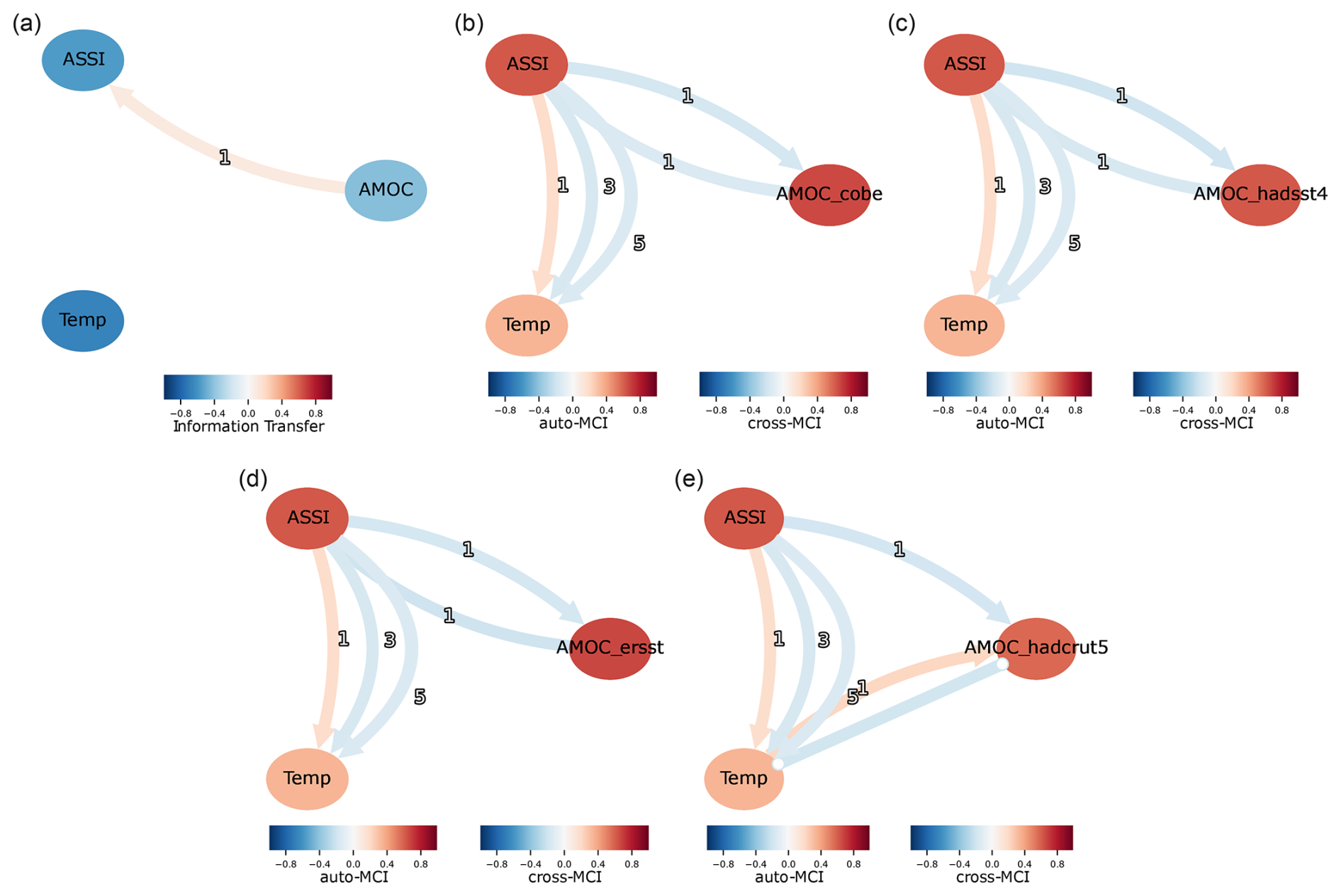
Figure F1 The causal networks as determined by (a) the LKIF method, (b–e) the PCMCI method for varying sea surface temperature datasets and corresponding AMOC indices.

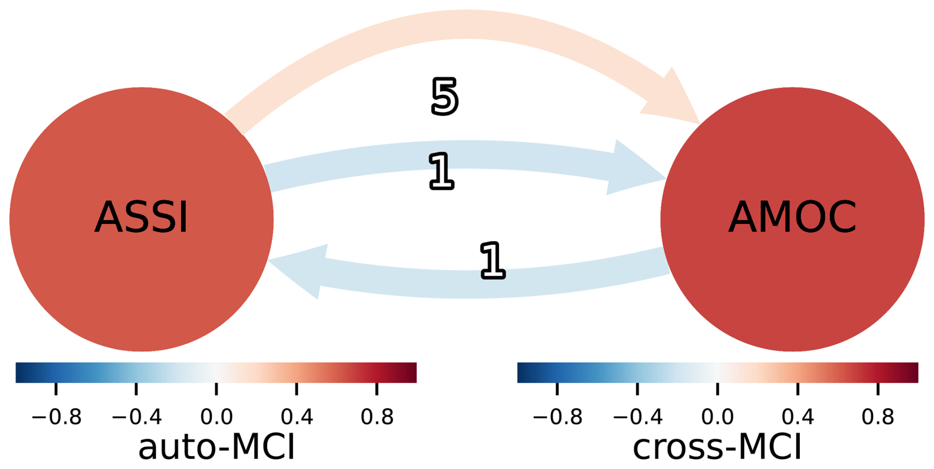
Figure F2 The causal network of the applied experiment (Fig. 5) without Arctic temperatures shows identical results.

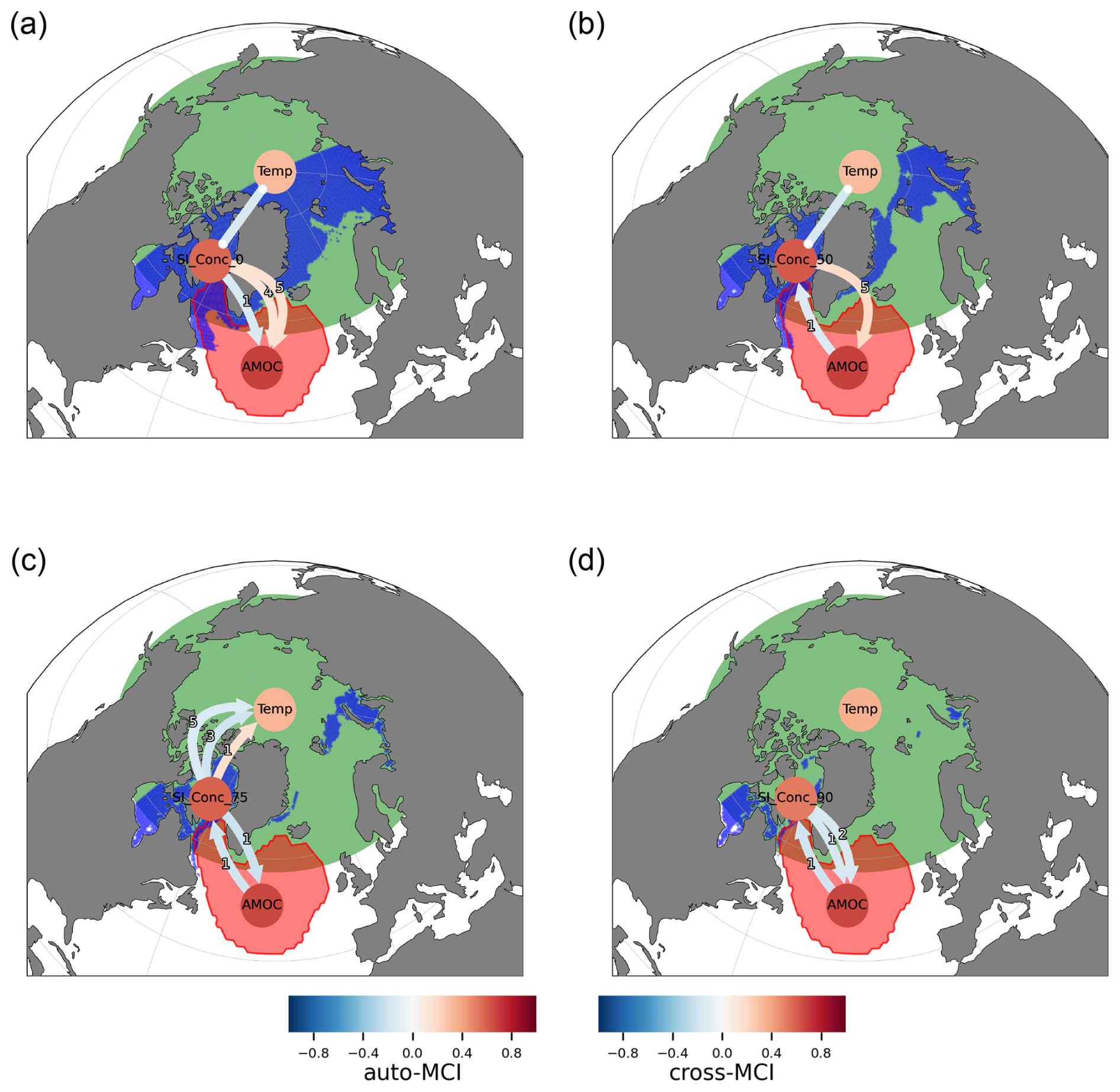
Figure F3 Causal inference results matching Fig. 5 for (a) full aggregation of sea ice, and aggregation of regions within the (b) 50th, (c) 75th, (d) 90th percentile of sea ice variance. The respective resulting aggregation areas are indicated in blue shading. The interaction of ASSI concentration and Arctic temperatures in (a), (b) is contemporaneous and thus with ambiguous direction.

Appendix G: Sensitivity Analyses for Noise Strength, Timesteps and Network Structure

The Wiener noise applied to each variable is scaled by a fixed σ, see Eq. (1). While the default value was set to 0.01 in previous experiments, here, we analyze the impact of the noise scale between 0.005–0.5 on prediction accuracy. Figure G1a implies no trend or impact of noise on the accuracy of any of the three causal inference methods up to a noise scale of σ=0.2. At a noise scale of 0.5, we observed noise-induced tipping events, which can explain the drop in performance in all methods. The remaining parameters are set to their default values for this experiment, and no forcing is applied.

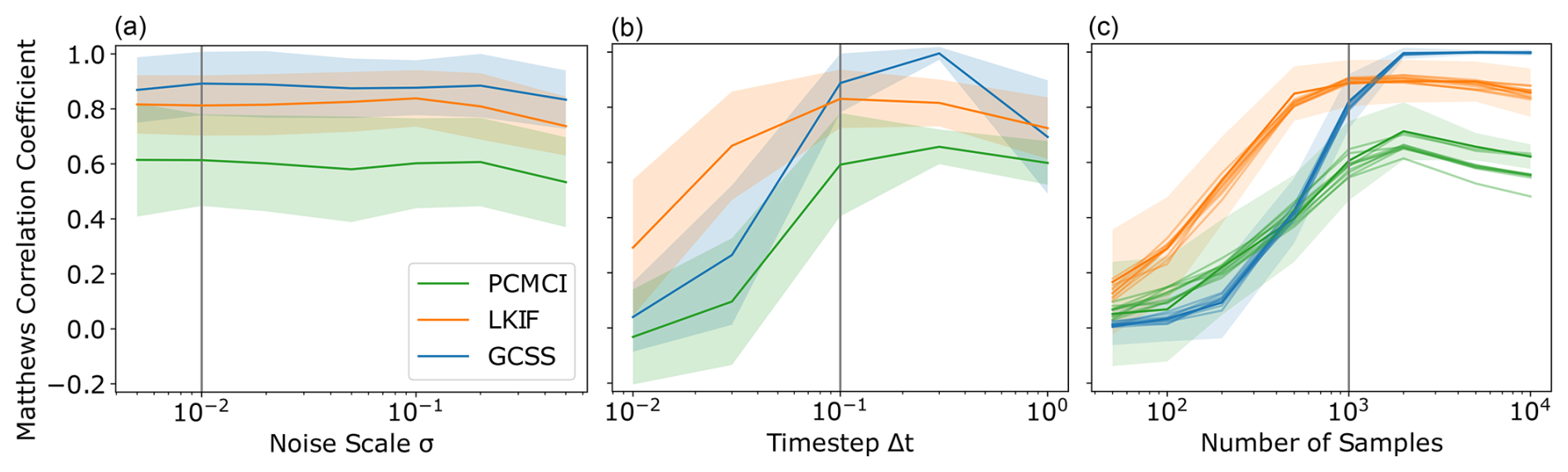
Figure G1 MCC scores in sensitivity tests for (a) the noise scale σ, and (b) the sampling timestep Δt. (c) MCC scores for randomized network structures under a changing number of samples, where each line corresponds to a single network. The high density network used in the study (Fig. A1d) is shown in full lines with shaded area indicating one standard deviation. Results on randomly generated networks of the same density are shown in shaded lines. In all panels, grey vertical lines indicate the respective default values.

Further, we test the sensitivity of results to the choice of Δt in the time discretization as described in Appendix B in the range of an order of magnitude in both directions. The results can be seen in Fig. G1b and show that the order of magnitude 0.1 is advantageous compared to smaller and larger Δt values, and results may only be improved slightly for GCSS with a slightly larger timestep. In applications to observational data, the intrinsic timescale of a system is usually not known in advance, thus optimizing the size of the timestep is not realistic in applied experiments.

For the manually designed networks in Fig. A1, we conduct another experiment to test the robustness of our results. As the default network (Fig. A1c) is designed rather specifically to contain one feedback loop and one non-interacting node, we instead conduct the analysis for the dense graph with six variables (Fig. A1d). We randomly generate 10 further network graphs, each with the same number of edges and feedback loops (12 edges, 11 cycles), with half of the edges weighted negative and positive, respectively. The new graphs are shown in Fig. G2. The resulting systems do not exhibit tipping events in the following experiment. We run the same experiment as in Fig. 2a of the main manuscript on the number of samples for each new network graph and show the results in Fig. G1c. The performances on similar randomly generated networks indeed stay within one standard deviation of the scores on the original network for all numbers of samples. For a number of networks, PCMCI performs worse for 5000 or more samples. This further supports the case for GCSS to be strongly preferable for high numbers of samples.

Figure G2 Random dense networks with 6 nodes, 12 edges and 11 cycles, as for the network shown in Fig. A1d used in the main manuscript.