Ensemble Kalman-guided model predictive path integral control for spatially localized suppression of extremes in chaotic geophysical flows

The possibility of influencing extreme weather phenomena has been discussed for decades; however, it remains far from operational practice, and there is still no established framework for designing small, spatially localized perturbations that can reliably steer chaotic geophysical flows. In this study, we propose a hybrid control method, termed ensemble-Kalman-guided model predictive path integral control (EKG-MPPI), which combines ensemble Kalman control (EnKC) with model predictive path integral (MPPI) control. Within a control simulation experiment framework, an ensemble Kalman filter is first used for state estimation, after which EnKC computes a candidate perturbation by treating the control objective as a pseudo-observation. An adaptive thresholding procedure then enforces spatial sparsity, so that the EnKC perturbation identifies candidate actuator locations and their nominal amplitudes. This information is embedded into the mean and covariance of Gaussian proposal distributions for MPPI, which subsequently refines the perturbation through sampling-based optimization with nonlinear rollouts, without linearizing the dynamics or computing gradients. Numerical experiments with the Lorenz-96 model and the surface quasi-geostrophic (SQG) model demonstrate that EKG-MPPI can suppress extremes in state variables and regional wind speed more effectively than EnKC alone, while using comparable or smaller control inputs. These results highlight EKG-MPPI as a promising building block for simulation-based assessment of localized intervention strategies in geophysical flows.

1 Introduction

The idea of deliberately influencing extreme weather phenomena, such as tropical cyclones (TCs), has been discussed for decades. However, it remains far from operational practice and there is still no established framework for designing small, spatially localized interventions with predictable effects. For example, Project STORMFURY attempted to weaken maximum wind speeds by artificially inducing convection around the TC eyewall, but its lack of effectiveness was reported by Willoughby et al. (1985). More recently, several studies have explored potential intervention mechanisms primarily in numerical modeling settings: based on simulations by Zhang et al. (2007), Cotton et al. (2007) discussed the possibility that mineral dust injection could suppress TC development, and Saharan dust has been shown to exert a strong influence on TCs. Furthermore, Latham et al. (2012) investigated TC weakening via sea-surface-temperature reduction, and Jacobson and Kempton (2014) demonstrated in simulations that arrays of offshore wind turbines can suppress near-surface wind speeds. A comprehensive review of these proposed approaches, together with feasibility and governance considerations, is provided by Miller et al. (2023). While these studies identify candidate actuators such as aerosols, mineral dust, and wind turbines, achieving concrete objectives (e.g., a substantial reduction in maximum wind speed) requires more than selecting an actuator type. It also calls for a mathematical framework that systematically optimizes where, when, and how strongly perturbations should be applied. This need is particularly acute because realistic anthropogenic influences are inherently local, weak, and intermittent. Therefore, it is crucial to devise methods that can efficiently identify “small perturbations” that can nevertheless meaningfully steer the evolution of chaotic geophysical flows, at least in simulation-based assessment settings.

An early step in this direction was taken by Henderson et al. (2005), who applied four-dimensional variational data assimilation (4D-Var), widely used in numerical weather prediction, to derive optimal initial perturbations for mitigating damage from tropical cyclones. This approach assumes that perturbations are applied only at the initial time. In contrast, Miyoshi and Sun (2022) proposed a framework in which small perturbations are applied continuously and adaptively. This concept, referred to as control simulation experiments (CSEs), has subsequently been employed and extended in later studies, including Kawasaki and Kotsuki (2024) and Ouyang et al. (2023), and has emerged as a practical approach for systematically evaluating the feasibility and potential side effects of candidate intervention strategies.

More recently, Sawada (2024b) introduced ensemble Kalman control (EnKC), which leverages the EnKF/EnKS framework to compute control increments by assimilating the control objective as a pseudo–observation, and demonstrated its effectiveness in numerical experiments with the Lorenz-63 model. Building on this, Sawada (2024a) proposed a strategy to reduce the magnitude of EnKC control inputs and to enforce spatial sparsity, with demonstrations in the Lorenz-96 model. While these studies Sawada (2024b, a) indicate that EnKC can identify effective perturbations, its computation relies on an approximate linearization of the dynamics over the prediction horizon, motivating strategies that can more fully exploit nonlinear dynamics.

To address the linearization limitation of EnKC while retaining a derivative-free formulation, we combine EnKC with model predictive path integral (MPPI) control. Like EnKC, MPPI is derivative-free; however, it evaluates candidate perturbations through nonlinear forward rollouts rather than linearized dynamics. At the same time, MPPI can be sample-inefficient when informative prior knowledge about the control distribution is unavailable, particularly in high-dimensional control spaces Power and Berenson (2022). We therefore introduce EnKC-guided MPPI (EKG-MPPI), which uses the sparse perturbations obtained from EnKC to construct an informative sampling distribution for MPPI. In this way, EnKC provides ensemble-based candidate perturbations that encode where control is likely to be effective and their nominal magnitude, while MPPI refines them via sampling-based optimization under the full nonlinear model without computing gradients. We demonstrate the effectiveness of the proposed method through numerical experiments with the Lorenz-96 model and the surface quasi-geostrophic (SQG) model.

This paper makes three contributions: (i) we propose EKG-MPPI, a hybrid framework that couples EnKC-based sparse actuation proposals with MPPI-based nonlinear refinement; (ii) we provide an explicit algorithmic formulation of EKG-MPPI, including a practical procedure for embedding EnKC-derived actuator locations and amplitudes into Gaussian sampling distributions for MPPI; and (iii) through numerical experiments with the Lorenz-96 and SQG models, we show that EKG-MPPI suppresses target extremes more strongly than EnKC while using comparable or smaller control inputs.

2 Preliminary Knowledge

This section reviews the Ensemble Kalman filter/control and Model Predictive Path Integral control.

2.1 Ensemble Kalman Filter (EnKF)

Let us first review the EnKF. Consider a discrete-time state–space system

$$\begin{array}{}\text{(1)}& {\displaystyle }{\mathit{x}}_t=M\left({\mathit{x}}_{t-\mathrm{1}}\right)+{\mathit{q}}_{t-\mathrm{1}},\text{(2)}& {\displaystyle }{\mathit{y}}_t^{\mathrm{o}}=\mathbf{H}\left({\mathit{x}}_t\right)+{\mathit{r}}_t,\end{array}$$

where x_t denotes the state vector, M the forecast model, q_t−1 the model error or the system noise, ${\mathit{y}}_t^{\mathrm{o}}$ the observation vector, H the observation operator, and r_t the observation error or the measurement noise. At an assimilation time t, the EnKF updates the model forecast by approximately minimizing the quadratic cost function

$$\begin{array}{}\text{(3)}& \begin{array}{rl}J\left({\mathit{x}}_t\right)& ={\displaystyle \frac{\mathrm{1}}{\mathrm{2}}}{\left({\mathit{x}}_t-{\stackrel{\mathrm{‾}}{\mathit{x}}}_t^{\mathrm{b}}\right)}^{\top }{\mathbf{P}}_{\mathrm{b}}^{-\mathrm{1}}\left({\mathit{x}}_t-{\stackrel{\mathrm{‾}}{\mathit{x}}}_t^{\mathrm{b}}\right)\\ & +{\displaystyle \frac{\mathrm{1}}{\mathrm{2}}}{\left({\mathit{y}}_t^{\mathrm{o}}-\mathbf{H}\left({\mathit{x}}_t\right)\right)}^{\top }{\mathbf{R}}^{-\mathrm{1}}\left({\mathit{y}}_t^{\mathrm{o}}-\mathbf{H}\left({\mathit{x}}_t\right)\right),\end{array}\end{array}$$

where ${\stackrel{\mathrm{‾}}{\mathit{x}}}_t^{\mathrm{b}}$ and P_b are the ensemble mean and background error covariance, and R is the observation error covariance matrix. The analysis ensemble $\mathit{\{}{\mathit{x}}_t^{a\left(i\right)}{\mathit{\}}}_{i=\mathrm{1}}^N$ is obtained by applying the EnKF update

$$\begin{array}{}\text{(4)}& {\displaystyle }{\mathit{x}}_t^{a\left(i\right)}={\mathit{x}}_t^{f\left(i\right)}+\mathbf{K}\left({\mathit{y}}_t^{o\left(i\right)}-\mathbf{H}\left({\mathit{x}}_t^{f\left(i\right)}\right)\right),\text{(5)}& {\displaystyle }\mathbf{K}={\mathbf{P}}_{\mathrm{b}}{\mathbf{H}}^{\top }{\left({\mathbf{HP}}_{\mathrm{b}}{\mathbf{H}}^{\top }+\mathbf{R}\right)}^{-\mathrm{1}},\end{array}$$

where ${\mathit{x}}_t^{f\left(i\right)}$ and ${\mathit{x}}_t^{a\left(i\right)}$ denote the ith forecast and analysis ensemble members, respectively, and H denotes the matrix representation of the (possibly linearized) observation operator H. In practice, the products P_bH^⊤ and HP_bH^⊤ are computed using ensemble statistics, so that the full covariance matrix P_b need not be formed explicitly. This ensemble representation enables the EnKF to handle high-dimensional systems efficiently. To mitigate sampling errors arising from the use of a finite ensemble, covariance localization is commonly employed. The localized Kalman gain is written as

$$\begin{array}{}\text{(6)}& \mathbf{K}=\mathit{\rho }\circ {\mathbf{P}}_{\mathrm{b}}{\mathbf{H}}^{\top }{\left(\mathit{\rho }\circ \left({\mathbf{HP}}_{\mathrm{b}}{\mathbf{H}}^{\top }\right)+\mathbf{R}\right)}^{-\mathrm{1}},\end{array}$$

where ∘ denotes the Schur (element-wise) product and

$$\begin{array}{}\text{(7)}& \mathit{\rho }=\exp [-d(i,j)/L]\end{array}$$

is a smooth correlation function defined in terms of the distance d(i,j) between grid points and a localization length scale L. This localization suppresses spurious long-range correlations, thereby improving the stability and accuracy of the EnKF updates.

Closely related to the EnKF is the ensemble Kalman smoother (EnKS), which extends the filter in time by estimating the state over an assimilation window using both past and future observations. Operationally, the EnKS can be implemented by propagating an ensemble forward with EnKF updates at each observation time and then applying a backward smoothing step that uses ensemble-based cross-covariances between states at different times and the observations. Readers interested in further details of the EnKF/EnKS family are referred to Houtekamer and Zhang (2016) for a comprehensive review.

2.2 Ensemble Kalman Control (EnKC)

EnKC builds directly on the EnKF and EnKS framework to formulate and solve an optimal control problem for various state-space (dynamical) systems. After the EnKF analysis at time t, let $\mathit{\{}{\mathit{x}}_t^{a\left(i\right)}{\mathit{\}}}_{i=\mathrm{1}}^N$ denote the analysis ensemble, with mean ${\stackrel{\mathrm{‾}}{\mathit{x}}}_t^{\mathrm{a}}$ and error covariance P_a. Over a prediction horizon T_EnKC, EnKC considers the quadratic cost function

$$\begin{array}{}\text{(8)}& \begin{array}{rl}{J}_{\mathrm{c}}\left({\mathit{x}}_t\right)& ={\displaystyle \frac{\mathrm{1}}{\mathrm{2}}}{\left({\mathit{x}}_t-{\stackrel{\mathrm{‾}}{\mathit{x}}}_t^{\mathrm{a}}\right)}^{\top }{\mathbf{P}}_a^{-\mathrm{1}}\left({\mathit{x}}_t-{\stackrel{\mathrm{‾}}{\mathit{x}}}_t^{\mathrm{a}}\right)\\ & +{\displaystyle \frac{\mathrm{1}}{\mathrm{2}}}{\left({\mathit{r}}_{t+T_{\text{EnKC}}}-{\mathbf{H}}_{\mathrm{c}}\left({\mathit{x}}_{t+T_{\text{EnKC}}}\right)\right)}^{\top }\\ & \times {\mathbf{R}}_{\mathrm{c}}^{-\mathrm{1}}\left({\mathit{r}}_{t+T_{\text{EnKC}}}-{\mathbf{H}}_{\mathrm{c}}\left({\mathit{x}}_{t+T_{\text{EnKC}}}\right)\right),\end{array}\end{array}$$

subject to the model dynamics

$$\begin{array}{}\text{(9)}& {\mathit{x}}_{k+\mathrm{1}}=M\left({\mathit{x}}_k\right),k=t,\mathrm{\dots },t+T_{\text{EnKC}}-\mathrm{1}.\end{array}$$

Here, ${\mathit{r}}_{t+T_{\text{EnKC}}}$ is a prescribed reference (target) vector at time t+T_EnKC, H_c maps the state variables to the control criteria (e.g., a regional average or maximum of a physical quantity), R_c is a user-defined weight (pseudo–observation error covariance), and ${\stackrel{\mathrm{‾}}{\mathit{x}}}_t^{\mathrm{a}}$ denotes the analysis ensemble mean. The first term penalizes the size of the perturbation to the initial analysis state, while the second term penalizes the mismatch between the predicted future state and the control objective. Assuming that the dynamics over the prediction horizon are approximately linear, the minimizer of J_c can be obtained by applying an EnKS. In this formulation, the reference vector ${\mathit{r}}_{t+T_{\text{EnKC}}}$ is assimilated as a “pseudo–observation” with error covariance R_c. The resulting EnKS analysis at time t,

$$\begin{array}{}\text{(10)}& {\mathit{x}}_t^{\mathrm{c}}={\stackrel{\mathrm{‾}}{\mathit{x}}}_t^{\mathrm{a}}+\mathbf{K}\left({\mathit{r}}_{t+T_{\text{EnKC}}}-{\mathbf{H}}_{\mathrm{c}}\left({\mathit{x}}_{t+T_{\text{EnKC}}}^{\mathrm{a}}\right)\right),\end{array}$$

yields the optimal perturbation ${\mathit{x}}_t^{\mathrm{c}}-{\stackrel{\mathrm{‾}}{\mathit{x}}}_t^{\mathrm{a}}$ to be applied to the system. The Kalman gain K is computed from the cross–covariance between the analysis ensemble at time t and the ensemble prediction at t+T_EnKC, and from the covariance of the projected prediction, in direct analogy with standard EnKF/EnKS formulations.

The EnKC algorithm can be summarized as follows:

1. Apply EnKF with real observations to obtain the analysis ensemble at time t.

2. From the analysis ensemble, perform ensemble forecasting up to t+T_EnKC and project the predicted states onto the control criteria via H_c.

3. Run EnKS, assimilating ${\mathit{r}}_{t+T_{\text{EnKC}}}$ as a pseudo–observation with error covariance R_c, and obtain the perturbation ${\mathit{x}}_t^{\mathrm{c}}-{\stackrel{\mathrm{‾}}{\mathit{x}}}_t^{\mathrm{a}}$.

4. Add this perturbation to the real system and to all analysis ensemble members, thereby updating the controlled “nature” and its ensemble representation.

5. Propagate the updated ensemble to the next data assimilation time. The resulting forecast serves as the new background for the next EnKF cycle, thus completing the loop and returning to Step 1.

In this way, EnKC integrates ensemble data assimilation and model predictive control by treating the control objective as a pseudo–observation within an EnKS framework, and by interpreting the resulting analysis increment as the optimal small perturbation to steer the system toward the desired future state. The control perturbation estimated by EnKC (Sawada, 2024a), ${\mathit{x}}_t^{\mathrm{c}}-{\stackrel{\mathrm{‾}}{\mathit{x}}}_t^{\mathrm{a}}$, has the same dimension as the full model state. In practical applications such as weather modification, however, it is unrealistic to apply perturbations to all state variables at every control step. It is therefore desirable to enforce spatial sparsity so that only a limited number of grid points (or regions) are actively perturbed, which naturally aligns with the interpretation of actuators placed at specific locations. Ideally, such sparsity can be promoted by augmenting the EnKC cost function with an ℓ₀-norm penalty:

$$\begin{array}{}\text{(11)}& \begin{array}{rl}{J}_{\mathrm{c}}\left({\mathit{x}}_t\right)& ={\displaystyle \frac{\mathrm{1}}{\mathrm{2}}}{\left({\mathit{x}}_t-{\stackrel{\mathrm{‾}}{\mathit{x}}}_t^{\mathrm{a}}\right)}^{\top }{\mathbf{P}}_a^{-\mathrm{1}}\left({\mathit{x}}_t-{\stackrel{\mathrm{‾}}{\mathit{x}}}_t^{\mathrm{a}}\right)\\ & +{\displaystyle \frac{\mathrm{1}}{\mathrm{2}}}{\left({\mathit{r}}_{t+T_{\text{EnKC}}}-{\mathbf{H}}_{\mathrm{c}}\left({\mathit{x}}_{t+T_{\text{EnKC}}}\right)\right)}^{\top }\\ & \times {\mathbf{R}}_{\mathrm{c}}^{-\mathrm{1}}\left({\mathit{r}}_{t+T_{\text{EnKC}}}-{\mathbf{H}}_{\mathrm{c}}\left({\mathit{x}}_{t+T_{\text{EnKC}}}\right)\right)\\ & +{\mathit{\lambda }}_{\mathrm{s}}\Vert {\mathit{x}}_t-{\stackrel{\mathrm{‾}}{\mathit{x}}}_t^{\mathrm{a}}{\Vert }_{\mathrm{0}},\end{array}\end{array}$$

where $\Vert \cdot {\Vert }_{\mathrm{0}}$ counts the number of nonzero elements (i.e., ℓ₀-norm) and λ_s controls the strength of the sparsity constraint. However, direct minimization of this objective is computationally demanding for high-dimensional systems, so an empirical yet effective strategy is adopted.

Following the idea of Schneider et al. (2022), we impose sparsity on the EnKC-estimated perturbation by applying a thresholding operator to its components. Specifically, after computing the standard EnKC update, we apply a thresholding operator T(θ) to each entry of ${\mathit{x}}_t^{\mathrm{c}}-{\stackrel{\mathrm{‾}}{\mathit{x}}}_t^{\mathrm{a}}$ so that small-magnitude components are discarded as noise and only sufficiently large perturbations are retained:

$$\begin{array}{}\text{(12)}& T\left(\mathit{\theta }\right)=\left\{\begin{array}{ll}\mathrm{0},& \text{if}\left|\mathit{\theta }\right|<\sqrt{\mathrm{2}{\mathit{\lambda }}_{\mathrm{s}}},\\ \mathit{\theta },& \text{otherwise}.\end{array}\right.\end{array}$$

While Schneider et al. (2022) treated $\sqrt{\mathrm{2}{\mathit{\lambda }}_{\mathrm{s}}}$ as a fixed hyperparameter, the present study adopts an adaptive formulation in which the threshold depends on the amplitude of the EnKC-derived perturbation at each control step. More precisely, the threshold parameter is updated as

$$\begin{array}{}\text{(13)}& \sqrt{\mathrm{2}{\mathit{\lambda }}_{\mathrm{s}}}=\mathrm{\Lambda }max\left|{\mathit{x}}_t^{\mathrm{c}}-{\stackrel{\mathrm{‾}}{\mathit{x}}}_t^{\mathrm{a}}\right|.\end{array}$$

where Λ is a user-specified coefficient that controls the enforced sparsity. This adaptive thresholding allows the sparsity level to automatically adjust to the magnitude of the EnKC-derived perturbations, thereby concentrating actuator effort on only the most influential grid points. In particular, choosing Λ=1 retains only the grid point with the largest perturbation, which is consistent with the actuator-placement interpretation in which localized increments indicate candidate actuator locations.

2.3 Model Predictive Path Integral Control (MPPI)

We next summarize the MPPI control framework. MPPI is a sample-based model predictive control (MPC) method grounded in probabilistic inference (Williams et al., 2018). MPPI considers the following nonlinear dynamical system:

$$\begin{array}{}\text{(14)}& {\mathit{x}}_{t+\mathrm{1}}=M({\mathit{x}}_t,{\mathit{u}}_t).\end{array}$$

At each time step, MPPI optimizes an open-loop control sequence over a finite horizon of length T. Let $\mathit{U}=({\mathit{u}}_{\mathrm{0}},{\mathit{u}}_{\mathrm{1}},\mathrm{\dots },{\mathit{u}}_{T-\mathrm{1}})$ denote the mean control sequence. MPPI introduces stochastic exploration by sampling control sequences $\mathit{V}=({\mathit{v}}_{\mathrm{0}},{\mathit{v}}_{\mathrm{1}},\mathrm{\dots },{\mathit{v}}_{T-\mathrm{1}})$ from a Gaussian distribution centered at U:

$$\begin{array}{}\text{(15)}& \mathit{q}(\mathit{V}\mid \mathit{U},\mathbf{\Sigma })=\prod _{\mathit{\tau }=\mathrm{0}}^{T-\mathrm{1}}\mathcal{N}({\mathit{v}}_{\mathit{\tau }};{\mathit{u}}_{\mathit{\tau }},\mathbf{\Sigma }),\end{array}$$

where $\mathbf{\Sigma }\in {\mathbb{R}}^{n_{\mathrm{u}}\times n_{\mathrm{u}}}$ is a user-specified positive definite covariance matrix. Equivalently, one may write ${\mathit{v}}_{\mathit{\tau }}={\mathit{u}}_{\mathit{\tau }}+{\mathit{ϵ}}_{\mathit{\tau }}$ with ${\mathit{ϵ}}_{\mathit{\tau }}\sim \mathcal{N}(\mathbf{0},\mathbf{\Sigma })$. Given a sampled control sequence V, the system is rolled out according to ${\mathit{x}}_{\mathit{\tau }+\mathrm{1}}=M({\mathit{x}}_{\mathit{\tau }},{\mathit{v}}_{\mathit{\tau }})$ (starting from the current state), and we define the total trajectory cost functional as

$$\begin{array}{}\text{(16)}& S\left(\mathit{V}\right)=\mathrm{\Phi }\left({\mathit{x}}_T\right)+\sum _{\mathit{\tau }=\mathrm{0}}^{T-\mathrm{1}}L({\mathit{x}}_{\mathit{\tau }},{\mathit{v}}_{\mathit{\tau }}).\end{array}$$

Under this setup, the stochastic optimal control problem at each time step is

$$\begin{array}{}\text{(17)}& {\mathit{U}}^{*}=\arg \underset{\mathit{U}\in \mathcal{U}}{min}{\mathbb{E}}_{\mathit{V}\sim \mathit{q}(\mathit{V}\mid \mathit{U},\mathbf{\Sigma })}\left[S\left(\mathit{V}\right)\right].\end{array}$$

MPPI can be derived via a variational free-energy bound. Let p(V) denote a base (prior) distribution over control sequences (typically chosen as a Gaussian), and define the free energy

$$\begin{array}{}\text{(18)}& F=-\mathit{\lambda }\log {\mathbb{E}}_{\mathit{V}\sim p}\left[\exp \left(-{\displaystyle \frac{S\left(\mathit{V}\right)}{\mathit{\lambda }}}\right)\right].\end{array}$$

Then, for any distribution r(V), the following inequality holds:

$$\begin{array}{}\text{(19)}& F\le {\mathbb{E}}_{\mathit{V}\sim \mathit{r}}\left[S\right(\mathit{V}\left)\right]+\mathit{\lambda }{D}_{\text{KL}}(\mathit{r}\Vert p),\end{array}$$

where D_KL is the Kullback–Leibler divergence. The minimizer of the right-hand side of Eq. (19) is the optimal distribution

$$\begin{array}{}\text{(20)}& {\mathit{q}}^{*}\left(\mathit{V}\right)={\displaystyle \frac{\mathrm{1}}{\mathit{\eta }}}\exp \left(-{\displaystyle \frac{S\left(\mathit{V}\right)}{\mathit{\lambda }}}\right)p\left(\mathit{V}\right),\end{array}$$

and substituting $\mathit{r}\left(\mathit{V}\right)={\mathit{q}}^{*}\left(\mathit{V}\right)$ into Eq. (19) yields equality (see Williams et al., 2018, for details). In practice, MPPI restricts r(V) to a Gaussian family with fixed covariance Σ and optimizes only the mean U. This corresponds to the KL projection

$$\begin{array}{}\text{(21)}& \widehat{\mathit{U}}=\arg \underset{\mathit{U}\in \mathcal{U}}{min}{D}_{\text{KL}}\left({\mathit{q}}^{*}\Vert \mathit{q}(\mathit{V}\mid \mathit{U},\mathbf{\Sigma })\right),\end{array}$$

whose minimizer satisfies, for fixed Σ,

$$\begin{array}{}\text{(22)}& \widehat{\mathit{U}}={\mathbb{E}}_{\mathit{V}\sim {\mathit{q}}^{*}}\left[\mathit{V}\right].\end{array}$$

Since direct sampling from q^* is intractable, we estimate Eq. (22) by Monte Carlo sampling with importance weights. When samples $\mathit{\{}{\mathit{V}}_k{\mathit{\}}}_{k=\mathrm{1}}^K$ are drawn from the base distribution p(V), Eq. (22) can be written as a normalized weighted average:

$$\begin{array}{}\text{(23)}& \widehat{\mathit{U}}\approx \sum _{k=\mathrm{1}}^K\stackrel{\mathrm{‾}}{\mathit{\omega }}\left({\mathit{V}}_k\right){\mathit{V}}_k,\end{array}$$

with log-weights and normalized weights

$$\begin{array}{}\text{(24)}& {\displaystyle }\mathit{\omega }\left({\mathit{V}}_k\right)& {\displaystyle }=-{\displaystyle \frac{\mathrm{1}}{\mathit{\lambda }}}S\left({\mathit{V}}_k\right),\text{(25)}& {\displaystyle }\stackrel{\mathrm{‾}}{\mathit{\omega }}\left({\mathit{V}}_k\right)& {\displaystyle }={\displaystyle \frac{\exp \left(\mathit{\omega }\right({\mathit{V}}_k\left)\right)}{{\sum }_{j=\mathrm{1}}^K\exp \left(\mathit{\omega }\right({\mathit{V}}_j\left)\right)}}.\end{array}$$

(If samples are drawn from a proposal distribution g(V)≠p(V), the weights are modified by the standard importance-sampling factor $p\left({\mathit{V}}_k\right)/g\left({\mathit{V}}_k\right)$.)

Typically, only the first element of the optimized control sequence $\widehat{\mathit{U}}$ is applied as the control input at each time step, after which the horizon is shifted forward and the procedure is repeated. As can be seen from Eq. (23) through Eq. (25), the weights for all samples can be computed in parallel, allowing efficient implementation on GPUs. Moreover, MPPI does not require gradient information of the dynamics or cost function and can be implemented using only forward simulations of the model.

3 EKG-MPPI: Proposed hybrid control method

3.1 Overall framework

EnKC provides a principled framework for determining small yet effective perturbations at each control step. However, EnKC computes the control increment by (approximately) linearizing the system dynamics over a finite prediction horizon, and its performance may therefore deteriorate when the dynamics are strongly nonlinear. To overcome this limitation, we propose a hybrid control scheme, termed EnKC-guided MPPI (EKG-MPPI), which combines EnKC with MPPI. In contrast to EnKC, MPPI evaluates candidate perturbations via nonlinear forward rollouts and thus can handle nonlinear dynamics without linearization. Nevertheless, as pointed out by Power and Berenson (2022), MPPI may suffer from poor sampling efficiency when applied without informative prior knowledge of the control distribution. This issue is particularly severe in high-dimensional geophysical systems, where the control space is large and naive sampling may fail to discover effective perturbations under a realistic computational budget.

EKG-MPPI addresses this issue by using the EnKC perturbation as prior information for MPPI. Intuitively, EnKC provides a sparse and physically informed guess of (i) where the system is most sensitive and (ii) how strongly it should be perturbed. We embed this information into the mean and variance (or covariance) of Gaussian sampling distributions, from which MPPI draws candidate actuator locations and magnitudes. MPPI then refines the perturbation through sampling-based optimization based on nonlinear rollouts, without any linearization or gradient computation.

The proposed EKG-MPPI scheme is implemented within the CSE framework, and the overall workflow is summarized in Fig. 1. At each data-assimilation time, we first apply the EnKF to assimilate observations and estimate the current state (Step 1). We then run EnKC using the analysis ensemble to obtain a sparse perturbation (Step 2). This perturbation is interpreted as a candidate actuator configuration and mapped to the parameters of Gaussian sampling distributions for actuator location and control magnitude. MPPI samples multiple candidate control inputs from these distributions, evaluates their performance over a prediction horizon, and computes a weighted average to obtain the final control input (Steps 3–4). In the CSE framework, the model trajectory obtained by integrating the forecast model without any control perturbation is referred to as the nature run, which serves as a proxy for the true atmosphere. The computed control is applied both to the nature run and to the analysis ensemble, after which the forecast–assimilation–control loop continues to the next time step.

Figure 1 Block diagram of the proposed EKG-MPPI.

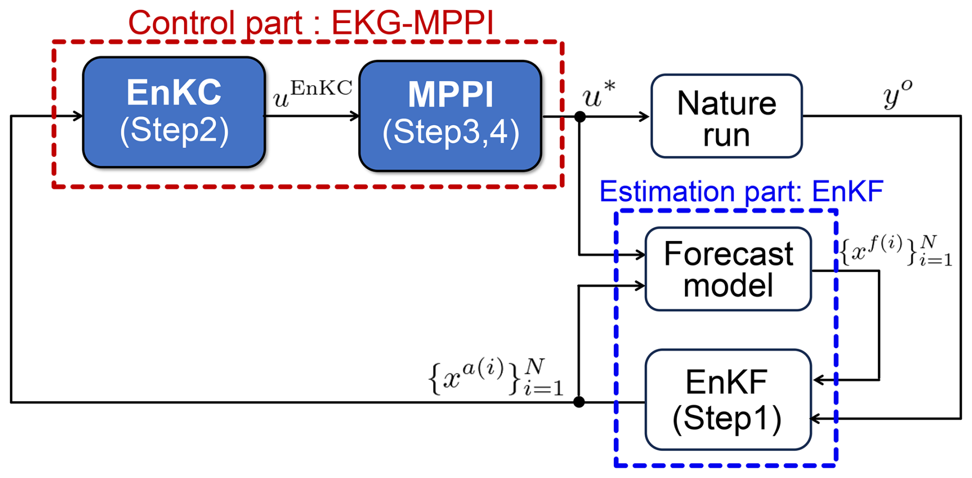
3.2 Algorithmic steps (Step 1–5)

In this section we describe the EKG-MPPI procedure at a single control time t. We denote the ensemble size by N and the current analysis ensemble by $\mathit{\{}{\mathit{x}}_t^{a\left(i\right)}{\mathit{\}}}_{i=\mathrm{1}}^N$.

Step 1: EnKF state estimation

As in standard CSE studies, accurate estimation of the system state is a prerequisite for effective control. At each assimilation time t, we apply the EnKF to assimilate the available observations ${\mathit{y}}_t^{\mathrm{o}}$ and update the forecast ensemble. The EnKF update is given in Sect. 2.1 and yields the analysis ensemble $\mathit{\{}{\mathit{x}}_t^{a\left(i\right)}{\mathit{\}}}_{i=\mathrm{1}}^N$. We then compute the analysis ensemble mean

$$\begin{array}{}\text{(26)}& {\stackrel{\mathrm{‾}}{\mathit{x}}}_t^{\mathrm{a}}={\displaystyle \frac{\mathrm{1}}{N}}\sum _{i=\mathrm{1}}^N{\mathit{x}}_t^{a\left(i\right)},\end{array}$$

which serves as the current state estimate used to initialize the subsequent control computation.

Step 2: EnKC-based control perturbation

In the second step, we apply EnKC (Sect. 2.2) to compute a control perturbation that will serve as prior information for MPPI. EnKC minimizes the quadratic cost function in Eq. (8) via an EnKS, interpreting the control objective as a pseudo–observation. The resulting control perturbation ${\mathit{x}}_t^{\mathrm{c}}-{\stackrel{\mathrm{‾}}{\mathit{x}}}_t^{\mathrm{a}}$ is then sparsified by the adaptive thresholding procedure described in Sect. 2.2. Among the information contained in the sparsified control vector, the key components for localized intervention are (i) the indices of its nonzero entries, which indicate candidate actuator locations, and (ii) the corresponding magnitudes, which represent nominal control amplitudes at those locations. To simplify the presentation, we set Λ=1 in Eq. (13), so that only the grid point with the largest perturbation remains nonzero. The resulting sparse control vector is denoted by ${\mathit{u}}_t^{\text{EnKC}}$, and encodes both the actuator location and its nominal control magnitude to be exploited by MPPI.

Step 3: EnKC-informed sampling of actuator location and magnitude

The third step embeds the information contained in ${\mathit{u}}_t^{\text{EnKC}}$ into the sampling distributions from which MPPI draws candidate control inputs. In this study, we parameterize each candidate actuator configuration by its location and magnitude. Let μ_loc,t and Σ_loc,t denote the mean and variance (scalar in the single-actuator case) that determine the sampling distribution of actuator locations, and let μ_mag,t and Σ_mag,t denote the corresponding quantities for the control magnitude. We define

$$\begin{array}{}\text{(27)}& \begin{array}{rlrl}{\displaystyle }& {\displaystyle }{\mathit{\mu }}_{\text{loc},t}=f_{\text{loc}}\left({\mathit{u}}_t^{\text{EnKC}}\right),& {\displaystyle }& {\displaystyle }{\mathbf{\Sigma }}_{\text{loc},t}=g_{\text{loc}}\left({\mathit{u}}_t^{\text{EnKC}}\right),\\ {\displaystyle }& {\displaystyle }{\mathit{\mu }}_{\text{mag},t}=f_{\text{mag}}\left({\mathit{u}}_t^{\text{EnKC}}\right),& {\displaystyle }& {\displaystyle }{\mathbf{\Sigma }}_{\text{mag},t}=g_{\text{mag}}\left({\mathit{u}}_t^{\text{EnKC}}\right),\end{array}\end{array}$$

where f_loc and f_mag map the EnKC output to the means of the sampling distributions for the actuator location and magnitude, respectively, and g_loc and g_mag define the corresponding sampling variances used by MPPI. Using the parameters in Eq. (27), we draw K_MPPI samples of actuator locations and magnitudes,

$$\begin{array}{}\text{(28)}& \begin{array}{rl}{\displaystyle }& {\displaystyle }{l}_{t,i}\sim \mathcal{G}(l\mid {\mathit{\mu }}_{\text{loc},t},{\mathbf{\Sigma }}_{\text{loc},t}),\\ {\displaystyle }& {\displaystyle }{m}_{t,i}\sim \mathcal{G}(m\mid {\mathit{\mu }}_{\text{mag},t},{\mathbf{\Sigma }}_{\text{mag},t}),i=\mathrm{1},\mathrm{2},\mathrm{\dots },{\mathbf{K}}_{\text{MPPI}},\end{array}\end{array}$$

where $\mathcal{G}(\cdot \mid \mathit{\mu },\mathbf{\Sigma })$ denotes a Gaussian distribution. Because actuator locations correspond to discrete grid indices, we round l_t,i to the nearest integer and clip it to the valid index range; with a slight abuse of notation, we denote the resulting index again by l_t,i. Each pair $(l_{t,i},m_{t,i})$ specifies one candidate actuator configuration for MPPI.

Step 4: MPPI rollout and importance weighting

In the fourth step, we evaluate the sampled actuator configurations via MPPI rollouts and compute their importance weights. Let ${\mathit{x}}_t={\stackrel{\mathrm{‾}}{\mathit{x}}}_t^{\mathrm{a}}$ denote the current state estimate (i.e., the state from which MPPI rolls out). Let n_u denote the dimension of the control input, and let ${\mathit{e}}_{\mathrm{\ell }}\in {\mathbb{R}}^{n_{\mathrm{u}}}$ be the ℓth standard basis vector. For each sample $(l_{t,i},m_{t,i})$, we construct a sparse control vector

$$\begin{array}{}\text{(29)}& {\mathit{u}}_{t,i}=m_{t,i}{\mathit{e}}_{l_{t,i}}.\end{array}$$

Starting from ${\mathit{x}}_{t,\mathrm{0}}^{\left(i\right)}={\mathit{x}}_t$, we propagate the system over the MPPI prediction horizon T_MPPI as

$$\begin{array}{}\text{(30)}& {\displaystyle }& {\displaystyle }{\mathit{x}}_{t,\mathrm{1}}^{\left(i\right)}=M\left({\mathit{x}}_{t,\mathrm{0}}^{\left(i\right)},{\mathit{u}}_{t,i}\right),\text{(31)}& {\displaystyle }& {\displaystyle }{\mathit{x}}_{t,\mathit{\tau }+\mathrm{1}}^{\left(i\right)}=M\left({\mathit{x}}_{t,\mathit{\tau }}^{\left(i\right)},\mathbf{0}\right),\mathit{\tau }=\mathrm{1},\mathrm{2},\mathrm{\dots },T_{\text{MPPI}}-\mathrm{1},\end{array}$$

where 0 denotes the zero control input. That is, the perturbation is applied only at the first rollout step, and no further input is provided during the remaining rollout. This reflects the single-step actuation setting used in our CSEs and also reduces the effective dimension of the control space, thereby improving sampling efficiency.

Let $S({\mathit{u}}_{t,i},{\mathit{x}}_t,M)$ be a state-dependent cost functional that quantifies the performance of the ith control sample. In our implementation, the EnKC-informed Gaussian distribution in Step 3 is used as the base distribution of MPPI, and therefore no importance-sampling correction term is required. The (unnormalized) log-weight is computed as

$$\begin{array}{}\text{(32)}& \mathit{\omega }\left({\mathit{u}}_{t,i}\right)=-{\displaystyle \frac{\mathrm{1}}{\mathit{\lambda }}}S({\mathit{u}}_{t,i},{\mathit{x}}_t,M),\end{array}$$

where λ is the temperature parameter in MPPI. The normalized weight is then computed as

$$\begin{array}{}\text{(33)}& {\stackrel{\mathrm{‾}}{w}}_{t,i}={\displaystyle \frac{\exp \left(\mathit{\omega }\right({\mathit{u}}_{t,i}\left)\right)}{{\sum }_{k=\mathrm{1}}^{{\mathbf{K}}_{\text{MPPI}}}\exp \left(\mathit{\omega }\right({\mathit{u}}_{t,k}\left)\right)}}.\end{array}$$

Finally, we first compute the weighted-average control vector

$$\begin{array}{}\text{(34)}& {\stackrel{\mathrm{̃}}{\mathit{u}}}_t=\sum _{i=\mathrm{1}}^{{\mathbf{K}}_{\text{MPPI}}}{\stackrel{\mathrm{‾}}{w}}_{t,i}{\mathit{u}}_{t,i},\end{array}$$

and then project it to a single-actuator (1-sparse) control by keeping only the largest-magnitude component:

$$\begin{array}{}\text{(35)}& {\displaystyle }& {\displaystyle }{l}_t^{\ast }=\arg \underset{\mathrm{\ell }}{max}\left|{\stackrel{\mathrm{̃}}{\mathit{u}}}_t\right(\mathrm{\ell }\left)\right|,\text{(36)}& {\displaystyle }& {\displaystyle }{\mathit{u}}_t^{\ast }={\stackrel{\mathrm{̃}}{\mathit{u}}}_t\left(l_t^{\ast }\right){\mathit{e}}_{l_t^{\ast }}.\end{array}$$

Algorithm 1 EKG-MPPI algorithm.

Require:

initial analysis ensemble $\mathit{\{}{\mathit{x}}_{\mathrm{0}}^{a\left(i\right)}{\mathit{\}}}_{i=\mathrm{1}}^N$; localization scale L; observation-error covariance matrix R; forecast model M; observation operator H; operator that maps the state variables to the control criteria H_c; control-weight matrix R_c; EnKC prediction horizon T_EnKC; MPPI prediction horizon T_MPPI; sparsity coefficient Λ; state-cost functional S; embedding functions $f_{\text{loc}},g_{\text{loc}},f_{\text{mag}},g_{\text{mag}}$; number of MPPI samples K_MPPI; temperature parameter λ; total number of assimilation steps T_sim.

1:

for $t=\mathrm{1},\mathrm{2},\mathrm{\dots },T_{\text{sim}}$ do

2:

Obtain observation ${\mathit{y}}_t^{\mathrm{o}}$.

3:

$\mathit{\{}{\mathit{x}}_t^{a\left(i\right)}{\mathit{\}}}_{i=\mathrm{1}}^N\leftarrow \mathbf{EnKF}\left(\mathit{\{}{\mathit{x}}_{t-\mathrm{1}}^{a\left(i\right)}{\mathit{\}}}_{i=\mathrm{1}}^N,{\mathit{y}}_t^{\mathrm{o}},L,\mathbf{R},M,\mathbf{H}\right)$.

4:

Compute the analysis ensemble mean ${\stackrel{\mathrm{‾}}{\mathit{x}}}_t^{\mathrm{a}}\leftarrow \frac{\mathrm{1}}{N}{\sum }_{i=\mathrm{1}}^N{\mathit{x}}_t^{a\left(i\right)}$.

5:

${\mathit{u}}_t^{\text{EnKC}}\leftarrow \mathbf{EnKC}\left(\mathit{\{}{\mathit{x}}_t^{a\left(i\right)}{\mathit{\}}}_{i=\mathrm{1}}^N,T_{\text{EnKC}},\mathrm{\Lambda },{\mathbf{R}}_{\mathrm{c}},M,{\mathbf{H}}_{\mathrm{c}}\right)$.

6:

Compute μ_loc,t, Σ_loc,t, μ_mag,t, Σ_mag,t according to Eq. (27).

7:

for $i=\mathrm{1},\mathrm{2},\mathrm{\dots },{\mathbf{K}}_{\text{MPPI}}$ do

8:

Sample $l_{t,i}\sim \mathcal{G}\left(l\mid {\mathit{\mu }}_{\text{loc},t},{\mathbf{\Sigma }}_{\text{loc},t}\right)$,
$m_{t,i}\sim \mathcal{G}\left(m\mid {\mathit{\mu }}_{\text{mag},t},{\mathbf{\Sigma }}_{\text{mag},t}\right)$.

9:

Construct a sparse control vector ${\mathit{u}}_{t,i}\leftarrow m_{t,i}{\mathit{e}}_{l_{t,i}}$, where e_ℓ denotes the ℓth standard basis vector.

10:

Evaluate the cost $S({\mathit{u}}_{t,i},{\stackrel{\mathrm{‾}}{\mathit{x}}}_t^{\mathrm{a}},M)$ and compute the (unnormalized) log-weight ω(u_t,i) using Eq. (32).

11:

end for

12:

Normalize the weights ${\stackrel{\mathrm{‾}}{w}}_{t,i}$ using Eq. (33).

13:

Compute the weighted-average control vector ${\stackrel{\mathrm{̃}}{\mathit{u}}}_t\leftarrow {\sum }_{i=\mathrm{1}}^{{\mathbf{K}}_{\text{MPPI}}}{\stackrel{\mathrm{‾}}{w}}_{t,i}{\mathit{u}}_{t,i}$.

14:

Select the actuator location $l_t^{\ast }\leftarrow \arg {max}_{\mathrm{\ell }}\left|{\stackrel{\mathrm{̃}}{\mathit{u}}}_t\right(\mathrm{\ell }\left)\right|$.

15:

Set the single-actuator control ${\mathit{u}}_t^{\ast }\leftarrow {\stackrel{\mathrm{̃}}{\mathit{u}}}_t\left(l_t^{\ast }\right){\mathit{e}}_{l_t^{\ast }}$.

16:

Apply ${\mathit{u}}_t^{\ast }$ to the nature run and update each analysis ensemble member via ${\mathit{x}}_t^{a\left(i\right)}\leftarrow {\mathit{x}}_t^{a\left(i\right)}+{\mathit{u}}_t^{\ast },i=\mathrm{1},\mathrm{\dots },N$.

17:

Advance the forecast model M to the next assimilation time.

18:

end for

Step 5: Feedback

In the final step, the optimal control ${\mathit{u}}_t^{\ast }$ computed in Eq. (36) is applied both to the nature run and to each member of the analysis ensemble, i.e.

$$\begin{array}{}\text{(37)}& {\mathit{x}}_t^{a\left(i\right)}\leftarrow {\mathit{x}}_t^{a\left(i\right)}+{\mathit{u}}_t^{\ast },i=\mathrm{1},\mathrm{2},\mathrm{\dots },N.\end{array}$$

The updated ensemble is then advanced by the forecast model until the next assimilation time, at which point the procedure returns to Step 1.

3.3 Pseudocode of EKG-MPPI

The EKG-MPPI procedure described above can be summarized by Algorithm 1, where EnKF (line 3) denotes the ensemble Kalman filter used for state estimation and EnKC (line 5) denotes the ensemble Kalman control scheme that computes sparse optimal perturbations as described in Sect. 2.2.

3.4 Single-step setting and motivation for MPPI

In the current implementation, the control perturbation is applied only at the first rollout step, and no further input is provided during the remaining horizon. The resulting optimization problem at each control decision is therefore effectively single-step. This approach is adopted as a proof of concept for localized intervention in chaotic flows and also reduces the effective dimension of the control space, thereby improving sampling efficiency. Nevertheless, we retain the MPPI formulation because rollout evaluation and importance-weight computation can be performed in parallel for a batch of samples, which is advantageous when forward simulation is the dominant computational cost. In addition, the same algorithmic framework extends naturally to multi-step control sequences and multiple actuators. To examine whether this choice remains competitive even in the present single-step setting, we provide a direct comparison with a standalone Bayesian optimization (BO) baseline (for details, see Sect. 4.1.2 and Appendix A).

4 Numerical Experiments

We demonstrate the effectiveness of EKG-MPPI through numerical experiments using the Lorenz-96 model and the SQG model.

4.1 Lorenz-96 model

Following the methodology of Sun et al. (2023) and Sawada (2024a), we conduct a control simulation experiment (CSE) aimed at mitigating extreme values in the Lorenz-96 system (Lorenz, 1995). The Lorenz-96 system is governed by

$$\begin{array}{}\text{(38)}& \begin{array}{rl}{\displaystyle }& {\displaystyle \frac{\mathrm{d}{X}_k}{\mathrm{d}t}}=(X_{k+\mathrm{1}}-X_{k-\mathrm{2}})X_{k-\mathrm{1}}-X_k+F,\\ {\displaystyle }& {\displaystyle }k\in \mathit{\{}\mathrm{1},\mathrm{2},\mathrm{\dots },\mathbf{K}\mathit{\}},\end{array}\end{array}$$

where K=40 in this study, and the external forcing parameter is set to F=8.0. Cyclic boundary conditions are imposed such that the indices are taken modulo K, i.e. $X_{k+\mathbf{K}}=X_k$. Equation (38) is numerically integrated using the fourth-order Runge–Kutta method with a time step of Δt=0.05. We perform numerical simulations over 160 600 model time steps. During the first 14 600 time steps, neither EnKC nor EKG-MPPI is applied; only EnKF is used to synchronize the estimated state with the uncontrolled nature run (spin-up period). Control is activated for the remaining 146 000 time steps, during which EnKF, EnKC, and EKG-MPPI are all executed. All diagnostics reported below are computed over this controlled period.

4.1.1 EnKC vs. EKG-MPPI

In this Section, we evaluate the effectiveness of the proposed EKG-MPPI method in comparison with EnKC. The hyperparameter settings for the two methods are as follows. For EnKC, observations are assumed to be available at every other grid point. The observation-error covariance matrix R is set to the identity matrix. The ensemble size is N=40, and the localization length scale is L=2. The prediction horizon is set to T_EnKC=0.2, corresponding to four time steps. The state threshold is set to ${\mathit{r}}_{t+T_{\text{EnKC}}}=\mathrm{12}$. The pseudo-observation matrix is defined so that grid points whose predicted states at time t+T_EnKC exceed the threshold are selected as observation points. The control-weight matrix R_c is set to 10⁻⁴.

For EKG-MPPI, the EnKC-related parameters are set identically to those of EnKC. In addition, the temperature parameter is set to λ=0.25, the number of samples is K_MPPI=40, and the MPPI prediction horizon is set to T_MPPI=4. The embedding functions in Eq. (27) are specified as

$$\begin{array}{}\text{(39)}& \begin{array}{rl}& f_{\text{loc}}\left({\mathit{u}}_t^{\text{EnKC}}\right)=\text{argnz}\left({\mathit{u}}_t^{\text{EnKC}}\right),\\ & g_{\text{loc}}\left({\mathit{u}}_t^{\text{EnKC}}\right)=\mathrm{5.0},\\ & f_{\text{mag}}\left({\mathit{u}}_t^{\text{EnKC}}\right)={\mathit{u}}_t^{\text{EnKC}}\left(f_{\text{loc}}\left({\mathit{u}}_t^{\text{EnKC}}\right)\right),\\ & g_{\text{mag}}\left({\mathit{u}}_t^{\text{EnKC}}\right)=\mathrm{0.1},\end{array}\end{array}$$

where argnz (⋅) returns the index of the nonzero entry of its argument. For the initial solution of MPPI, we adopt the perturbations obtained by EnKC, as represented by f_loc and f_mag. The running state-cost function is defined as

$$\begin{array}{}\text{(40)}& S\left({\mathit{x}}_t\right)=\Vert max({\mathit{x}}_t-\mathrm{12},\mathrm{0}){\Vert }_{\mathrm{1}}.\end{array}$$

Under these settings, we conducted 10 simulations with different random seeds. For each method, we computed the mean and standard deviation over the 10 runs of (i) the number of state components exceeding the threshold value of 12 and (ii) the control-input magnitude. The results are summarized in Table 1. EKG-MPPI achieved a lower extreme-event count (7622±146) than EnKC (7820±142), while also requiring a smaller control-input magnitude (0.166±0.002 for EKG-MPPI versus 0.191±0.001 for EnKC).

Table 1 Comparison of EKG-MPPI and EnKC in the Lorenz-96 control simulation experiment. The second column reports the extreme-event count, defined as $\mathit{\#}\mathit{\left\{}\right(t,k):X_{t,k}\ge \mathrm{12}\mathit{\}}$, where #{⋅} denotes set cardinality. The third column reports the input magnitude, defined as $\frac{\mathrm{1}}{N_{\text{ctrl}}}\sum _{t\in {\mathcal{T}}_{\text{ctrl}}}\sum _k\left|{\mathit{u}}_{t,k}\right|$, where 𝒯_ctrl denotes the set of time steps at which control is applied during the simulation horizon T_sim, and $N_{\text{ctrl}}=\left|{\mathcal{T}}_{\text{ctrl}}\right|$. All values are shown as mean ± standard deviation over 10 simulations with different random seeds.

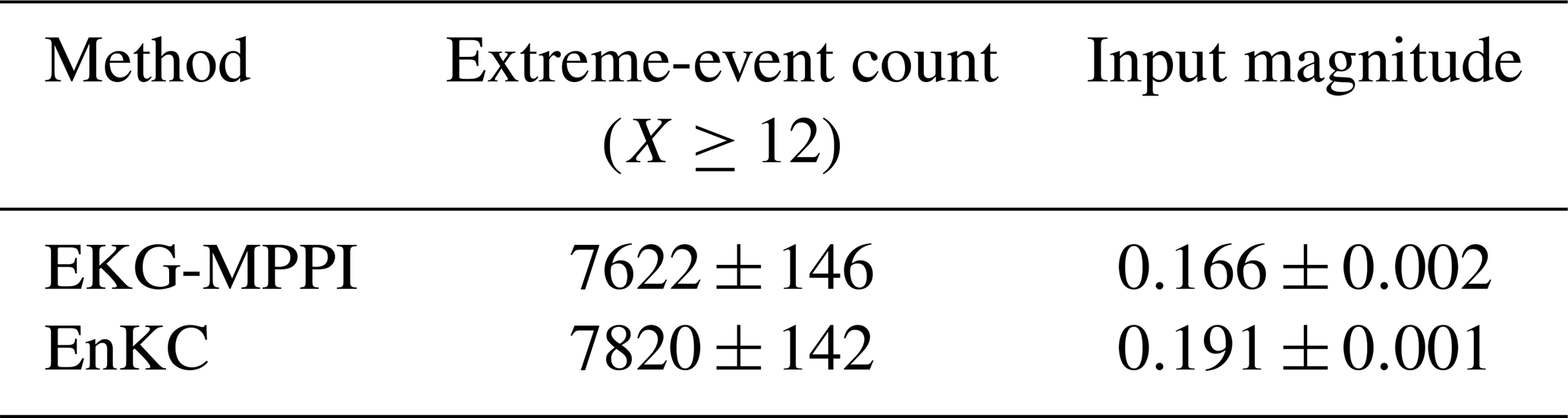
These results demonstrate that EKG-MPPI outperforms EnKC in terms of both suppressing extreme events and reducing control effort. We attribute the improvement over EnKC to the nonlinear evaluation introduced in the MPPI refinement stage.

4.1.2 Comparison with Bayesian optimization in the single-step setting

Since the control perturbation is applied only at the first rollout step, the optimization performed at each control decision reduces to the selection of a single localized perturbation. Bayesian optimization (BO) is a standard framework for sample-efficient optimization of expensive black-box functions (see, e.g., Shahriari et al., 2016), and thus it provides a natural baseline for the present single-step setting. We therefore compare EKG-MPPI with a standalone BO controller to assess whether the MPPI-based formulation remains advantageous even in this simplified setting. For a fair comparison, the BO baseline optimizes the same single-step control parameterization as EKG-MPPI, using the same prediction horizon and the same state-cost function.

The objective function used by the BO baseline is designed to balance the severity of extreme events against the intervention cost. Specifically, the cost function is defined as

$$\begin{array}{}\text{(41)}& c({\mathit{x}}_t,{\mathit{u}}_t)=\sum _{i=\mathrm{1}}^{T_{\text{BO}}}\sum _{j=\mathrm{1}}^{\mathbf{K}}max\left({\mathit{x}}_{t+i}^{\left(j\right)}-{\mathit{r}}_{\text{th}},\mathrm{0}\right)+\mathit{\alpha }\Vert {\mathit{u}}_t{\Vert }_{\mathrm{1}},\end{array}$$

where ${\mathit{x}}_{t+i}^{\left(j\right)}$ denotes the jth component of the predicted state, K is the state dimension, and T_BO is the prediction horizon. The state trajectory is obtained by propagating the model dynamics as

$$\begin{array}{}\text{(42)}& \begin{array}{rl}{\displaystyle }{\mathit{x}}_{t+\mathrm{1}}& {\displaystyle }=M({\mathit{x}}_t+{\mathit{u}}_t),\\ {\displaystyle }{\mathit{x}}_{t+i}& {\displaystyle }=M\left({\mathit{x}}_{t+i-\mathrm{1}}\right),i=\mathrm{2},\mathrm{\dots },T_{\text{BO}}.\end{array}\end{array}$$

The first term measures the cumulative exceedance above the threshold over the prediction horizon, while the second term penalizes the intervention magnitude. The parameter α controls the trade-off between intervention effectiveness and intervention cost. We employ the Expected Improvement (EI) acquisition function Jones et al. (1998), set the search interval to $[-\mathrm{1},\mathrm{1}]$, use α=1, and perform 7 BO iterations at each control decision. Although this is a modest BO budget, it already leads to a substantially larger computation time per decision than that of EKG-MPPI; see Table 3 for the runtime comparison.

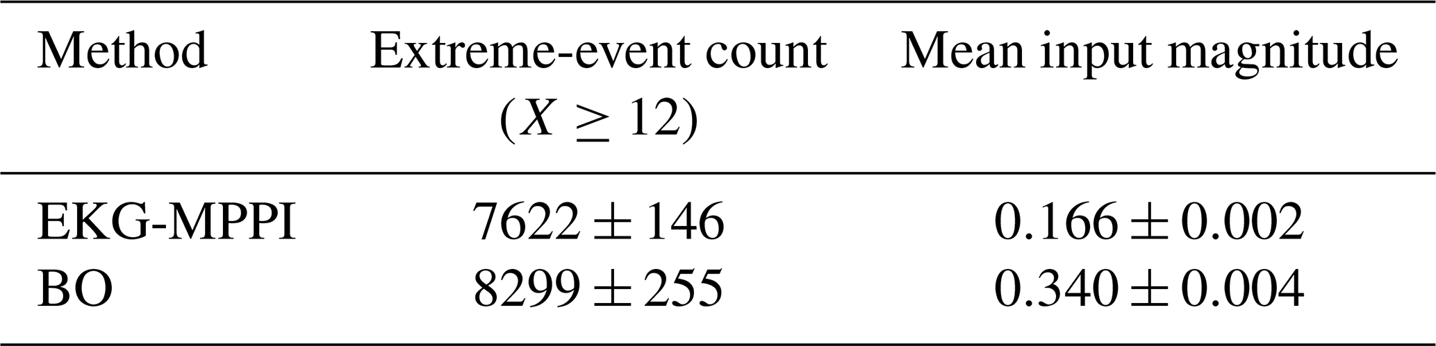
Table 2 summarizes the results. As in Sect. 4.1.1, the experiments are repeated over 10 different random seeds. EKG-MPPI yields fewer extreme events than BO (7622±146 vs. 8299±255) and a smaller mean control-input magnitude (0.166±0.002 vs. 0.340±0.004). These results indicate that EKG-MPPI remains effective in the present single-step setting, outperforming the standalone BO baseline in both reported metrics. For completeness, Appendix A reports the corresponding comparison between standalone BO and vanilla MPPI under the same single-step setting.

Table 2 Comparison between EKG-MPPI and a standalone BO baseline in the single-step Lorenz-96 control setting. The second and third columns report the extreme-event count and the mean input magnitude, respectively, defined in the same manner as in Table 1.

4.1.3 BO-informed prior vs. EnKC-informed prior in MPPI

To further examine the prior design used in EKG-MPPI, we introduce an additional baseline, denoted BO-MPPI, in which Bayesian optimization is used to estimate the intervention location and magnitude that define the prior supplied to MPPI. Unlike the standalone BO baseline in Sect. 4.1.2, the purpose of this comparison is not to contrast BO with EKG-MPPI. Rather, because BO-MPPI and EKG-MPPI share the same MPPI refinement stage, this comparison isolates the effect of the prior used to guide MPPI. BO-MPPI therefore serves as an ablation baseline for the prior construction.

For the BO component of BO-MPPI, the optimization iterations and the search interval for the intervention are set in the same way as in Sect. 4.1.2. The hyperparameters of EKG-MPPI are set as in Sect. 4.1.1. Under these settings, for each $\mathit{\lambda }\in \mathit{\{}\mathrm{0.1},\mathrm{1.0},\mathrm{10}\mathit{\}}$, we conduct experiments by varying the BO-MPPI parameter α over $\mathit{\{}\mathrm{0.01},\mathrm{0.1},\mathrm{1},\mathrm{10},\mathrm{100}\mathit{\}}$. For ease of visualization, both the average intervention magnitude and the intervention-effectiveness metric are rescaled; see Appendix B for details.

Figure 2 compares EKG-MPPI and BO-MPPI for $\mathit{\lambda }\in \mathit{\{}\mathrm{0.1},\mathrm{1.0},\mathrm{10}\mathit{\}}$. In each panel, the EKG-MPPI result is located below the empirical lower envelope, i.e., the Pareto-like trade-off curve, formed by the BO-MPPI results obtained by varying α. This indicates that, for a comparable level of intervention effectiveness, EKG-MPPI achieves a smaller average intervention magnitude than BO-MPPI. In other words, the EnKC-informed prior yields a more favorable trade-off between intervention effectiveness and control magnitude than the BO-informed prior across the tested values of λ. These results suggest that the advantage of EKG-MPPI is robust to the choice of λ rather than being driven by a particular hyperparameter setting.

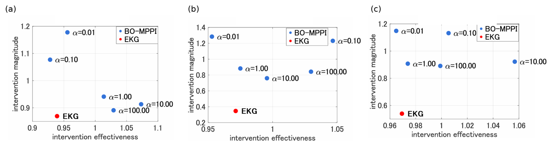
Figure 2 Comparison between BO-MPPI and EKG-MPPI for different values of λ: (a) λ=0.1, (b) λ=1.0, and (c) λ=10.

4.1.4 Sensitivity analysis of EKG-MPPI hyperparameters

We next examine the sensitivity of EKG-MPPI to its two main hyperparameters: the temperature parameter λ and the number of MPPI samples K_MPPI. We vary λ over $\mathit{\{}\mathrm{10},\mathrm{1},\mathrm{0.1},\mathrm{0.01},\mathrm{0.001}\mathit{\}}$ and K_MPPI over $\mathit{\{}\mathrm{5},\mathrm{10},\mathrm{20},\mathrm{40},\mathrm{80}\mathit{\}}$. For each configuration, we record the number of threshold exceedances, the mean control-input magnitude, and the number of time steps at which control is applied. The results are shown in Fig. 3.

Figure 3 shows a clear overall tendency: decreasing λ increases the mean control-input magnitude while reducing the frequency of control application. In MPPI, λ determines how strongly the importance weights concentrate on low-cost samples. Smaller values of λ therefore produce more peaked weights and drive the update toward more aggressive perturbations identified in the sampled rollouts. In EKG-MPPI, the sampling distribution is centered on the EnKC-informed proposal ${\mathit{u}}_t^{\mathrm{EnKC}}$. A smaller λ thus induces a stronger shift away from this EnKC-guided proposal toward samples with particularly low rollout cost. This tendency becomes more pronounced when λ is very small (e.g., 0.01 or 0.001). In that regime, increasing K_MPPI tends to further increase the mean control-input magnitude and decrease the control frequency. A plausible explanation is that a larger sample set more often contains rare but highly effective perturbations; when λ is small, the weight update becomes strongly concentrated on such samples, thereby amplifying the resulting control magnitude. Figure 3 also indicates that smaller λ and larger K_MPPI generally reduce the number of threshold exceedances, suggesting stronger suppression of extremes. At the same time, the mean input magnitude exhibits a non-monotonic dependence on λ, with the smallest value occurring around λ=1 in the present experiment. Although one might expect a larger value such as λ=10 to yield smaller inputs, an excessively large λ produces diffuse weights and hence overly conservative updates. Such conservative control may allow extremes to persist, which can in turn require larger or more sustained interventions later.

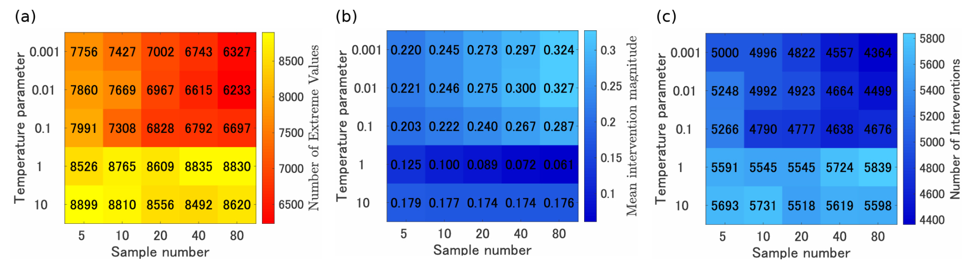
Figure 3 Hyperparameter configuration maps displaying the effects of varying λ and sample size on control outcomes: (a) number of threshold exceedances, (b) mean control-input magnitude, and (c) number of time steps at which control is applied.

4.1.5 Computation time

We next compare the computation time of EnKC, BO, BO-MPPI, and EKG-MPPI. For EnKC, BO and EKG-MPPI, the parameter settings are the same as those in Sect. 4.1.1 and in Sect. 4.1.2. For BO-MPPI, the search interval for the intervention is set to $[-\mathrm{1.0},\mathrm{1.0}]$, and the number of BO iterations is set to 7. At each control decision, we measure the time required to compute the control input and summarize it by its mean and standard deviation. The results are listed in Table 3. For EKG-MPPI, the mean runtime per control decision is $(\mathrm{6.30}\pm \mathrm{5.23})\times {\mathrm{10}}^{-\mathrm{5}}\mathrm{s}$ for the EnKC part and $(\mathrm{3.24}\pm \mathrm{1.17})\times {\mathrm{10}}^{-\mathrm{4}}\mathrm{s}$ for the MPPI rollout and weight computation, giving a total mean runtime of $\mathrm{3.87}\times {\mathrm{10}}^{-\mathrm{4}}\mathrm{s}$ per decision. Thus, approximately 16 % of the runtime is attributable to the EnKC part and 84 % to the MPPI part. This indicates that the dominant computational cost in EKG-MPPI arises from rollout evaluation rather than from construction of the EnKC-informed prior. The additional overhead introduced by the prior estimation is therefore modest in the present setting. Table 3 also shows that EKG-MPPI is substantially faster than BO-MPPI. The mean runtime of BO-MPPI is 0.216±0.104 s per control decision, whereas the total mean runtime of EKG-MPPI is $\mathrm{3.87}\times {\mathrm{10}}^{-\mathrm{4}}\mathrm{s}$, making BO-MPPI approximately 5.6×10² times slower in the present experiment. Moreover, the total runtime of EKG-MPPI is much shorter than one model time step, Δt=0.05, indicating that the method is computationally feasible for the present online-control setting. Finally, the present experiment uses K_MPPI=40 samples. Under ideal parallel execution, the MPPI component could in principle be reduced to approximately one-fortieth of its current runtime, i.e., about $\mathrm{8.1}\times {\mathrm{10}}^{-\mathrm{6}}\mathrm{s}$. This observation further suggests that EKG-MPPI is well suited to parallel hardware when forward rollout evaluation dominates the computational cost.

Table 3 Mean computation time per control decision (mean ± standard deviation). For EKG-MPPI, the runtime is decomposed into the EnKC-based prior construction part and the MPPI rollout/weight computation part.

4.2 Surface quasi-geostrophic model

The quasi-geostrophic (QG) model is a standard framework for describing mesoscale barotropic and baroclinic dynamics; for a comprehensive review, see Vallis (2017). The surface quasi-geostrophic (SQG) model is derived from the QG model under the assumption of uniform interior potential vorticity. A key feature of the SQG model is that the surface buoyancy acts as an active tracer from which the horizontal velocity field is diagnosed. All numerical experiments follow the setup and parameter values in Resseguier et al. (2017).

4.2.1 SQG dynamics and diagnostic velocity

Let b(x,t) denote the surface buoyancy on a doubly periodic domain $\mathit{x}=(\mathit{x},\mathit{y})\in {\mathbb{T}}^{\mathrm{2}}$. In the SQG model, b evolves as an active tracer and the velocity is diagnosed from b via a streamfunction ψ:

$$\begin{array}{}\text{(43)}& {\displaystyle }& {\displaystyle }{\partial }_{t}b+\mathit{v}\cdot \mathrm{\nabla }b=\mathcal{D}\left(b\right)+f,\text{(44)}& {\displaystyle }& {\displaystyle }\mathit{v}={\mathrm{\nabla }}^{⟂}\mathit{\psi }=(-{\partial }_y\mathit{\psi },{\partial }_x\mathit{\psi }),\text{(45)}& {\displaystyle }& {\displaystyle }b=(-\mathrm{\Delta }{)}^{\mathrm{1}/\mathrm{2}}\mathit{\psi }.\end{array}$$

Here 𝒟(b) denotes a dissipation operator and f is an external forcing term. Equivalently, in Fourier space, $\widehat{\mathit{\psi }}\left(\mathit{k}\right)=\left|\mathit{k}{|}^{-\mathrm{1}}\widehat{b}\right(\mathit{k})$ for k≠0, with the mean mode set to zero; see Resseguier et al. (2017) for numerical implementation details. We discretize b on a 128×128 grid and denote the vectorized buoyancy field at discrete time t by x_t∈ℝⁿ with n=128². Let $M_{\mathrm{0}}:{\mathbb{R}}^n\to {\mathbb{R}}^n$ be the one-step forecast model corresponding to the numerical time integrator of Eq. (43) (including the SQG inversion in Eq. 45):

$$\begin{array}{}\text{(46)}& {\mathit{x}}_{t+\mathrm{1}}=M_{\mathrm{0}}\left({\mathit{x}}_t\right).\end{array}$$

It is assumed that the surface buoyancy can be controlled via a small, spatially localized increment. Accordingly, we model the actuation as an additive perturbation applied at the control time t:

$$\begin{array}{}\text{(47)}& {\mathit{x}}_t^{+}={\mathit{x}}_t+{\mathit{u}}_t,\end{array}$$

followed by the uncontrolled model integration. Thus, the controlled forecast model M used in Step 4 (Sect. 3.2) is defined by

$$\begin{array}{}\text{(48)}& M({\mathit{x}}_t,{\mathit{u}}_t)=M_{\mathrm{0}}({\mathit{x}}_t+{\mathit{u}}_t),M({\mathit{x}}_t,\mathrm{0})=M_{\mathrm{0}}\left({\mathit{x}}_t\right).\end{array}$$

This is consistent with the single-step actuation setting assumed in Step 4 (Sect. 3.2), where the perturbation is applied only at the first rollout step and no further input is provided during the remaining rollout. We consider a single localized actuator at each control time. Let ${\mathit{l}}_{\mathit{t}}=(i_t,j_t)$ denote the actuator location on the 128×128 grid and m_t∈ℝ its magnitude. Let ${\mathit{e}}_{{\mathit{l}}_{\mathit{t}}}\in {\mathbb{R}}^n$ be the standard basis vector corresponding to grid point l_t (i.e., a Kronecker delta on the vectorized grid). The control input is then

$$\begin{array}{}\text{(49)}& {\mathit{u}}_t=m_t{\mathit{e}}_{{\mathit{l}}_{\mathit{t}}}.\end{array}$$

In the EKG-MPPI/MPPI sampling step, l_t is sampled in ℝ² and then rounded to the nearest integer grid index and clipped to the valid range in each coordinate, following the same discretization convention as in Sect. 3.2. Given a buoyancy state x_t, we diagnose the streamfunction and velocity using Eq. (44) through Eq. (45), and define the wind-speed magnitude field as

$$\begin{array}{}\text{(50)}& w\left({\mathit{x}}_t\right)\left(\mathit{x}\right)=\Vert \mathit{v}\left({\mathit{x}}_t\right)\left(\mathit{x}\right){\Vert }_{\mathrm{2}}.\end{array}$$

Let Ω_tar denote a prescribed target region (a set of grid points). Our control objective is to suppress wind speed within Ω_tar, and we define the running state-cost function as

$$\begin{array}{}\text{(51)}& S\left({\mathit{x}}_t\right)=\text{target}\left(w\right({\mathit{x}}_t\left)\right),\end{array}$$

where target (⋅) aggregates wind speed within Ω_tar (e.g., regional mean or maximum). See Resseguier et al. (2017) for numerical details of the SQG inversion and the diagnostic computation of w(⋅).

4.2.2 Simulation Results

To compare the control performance of EKG-MPPI and EnKC, we conduct control simulations on a 128×128 grid map under eight different target regions: $[\mathrm{85},\mathrm{95}]\times [\mathrm{85},\mathrm{95}]$, $[\mathrm{85},\mathrm{95}]\times [\mathrm{90},\mathrm{100}]$, $[\mathrm{85},\mathrm{95}]\times [\mathrm{95},\mathrm{105}]$, $[\mathrm{90},\mathrm{100}]\times [\mathrm{85},\mathrm{95}]$, $[\mathrm{90},\mathrm{100}]\times [\mathrm{90},\mathrm{100}]$, $[\mathrm{90},\mathrm{100}]\times [\mathrm{95},\mathrm{105}]$, $[\mathrm{95},\mathrm{105}]\times [\mathrm{85},\mathrm{95}]$ and $[\mathrm{95},\mathrm{105}]\times [\mathrm{90},\mathrm{100}]$. Hereafter, these experiments are referred to as exp1 through exp8. For each scenario, five simulations are conducted using different random seeds, resulting in a total of 40 simulations. The mean and standard deviation of the maximum wind speed and the average intervention amount are then computed for comparison. The total number of simulation steps in each run is set to 10 118, which corresponds to approximately 10 d of real time. For EnKC, the ensemble size is set to N=40, the prediction horizon is set to T_EnKC=500 steps (approximately 12 h), and the control weight is set to 10. For EKG-MPPI, the number of samples is set to K_MPPI=40, and the prediction horizon is also set to 500 steps. The embedding function into the prior distribution is defined as follows:

$$\begin{array}{}\text{(52)}& \begin{array}{rl}& f_{\text{loc}}\left({\mathit{u}}_t^{\text{EnKC}}\right)=\text{argnz}\left({\mathit{u}}_t^{\text{EnKC}}\right),\\ & g_{\text{loc}}\left({\mathit{u}}_t^{\text{EnKC}}\right)=\mathrm{10.0},\\ & f_{\text{mag}}\left({\mathit{u}}_t^{\text{EnKC}}\right)={\mathit{u}}_t^{\text{EnKC}}\left(f_{\text{loc}}\left({\mathit{u}}_t^{\text{EnKC}}\right)\right),\\ & g_{\text{mag}}\left({\mathit{u}}_t^{\text{EnKC}}\right)={∥{\mathit{u}}_t^{\text{EnKC}}∥}_{\mathrm{1}}^{\mathrm{2}},\end{array}\end{array}$$

The state cost function for EKG-MPPI is defined as follows:

$$\begin{array}{}\text{(53)}& S\left({\mathit{x}}_t\right)=max\left(\text{target}\right(w\left({\mathit{x}}_t\right))-w_{\text{th}},\mathrm{0})\end{array}$$

where w(⋅) is a function that converts the buoyancy state x_t into the corresponding wind speed, and target (⋅) is a function that computes the magnitude of the wind speed within the target region. Here w_th denotes the wind speed threshold, and in this study we set w_th=2. For details of the function w(⋅), the reader is referred to Resseguier et al. (2017).

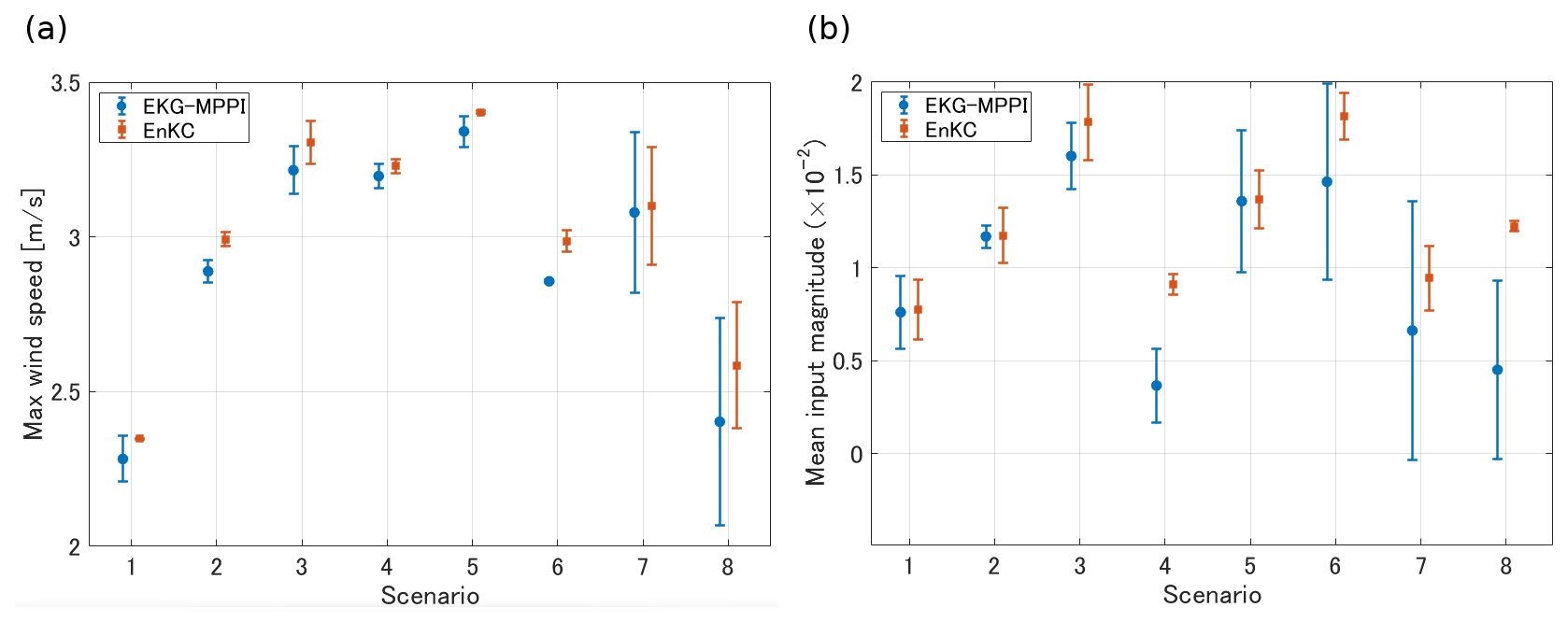
Figure 4 Mean and standard deviation of (a) the maximum wind speed and (b) the mean input magnitude for each scenario. Smaller values indicate better performance in terms of extreme-event suppression and control effort, respectively. The panels display raw values for each scenario rather than percentage differences.

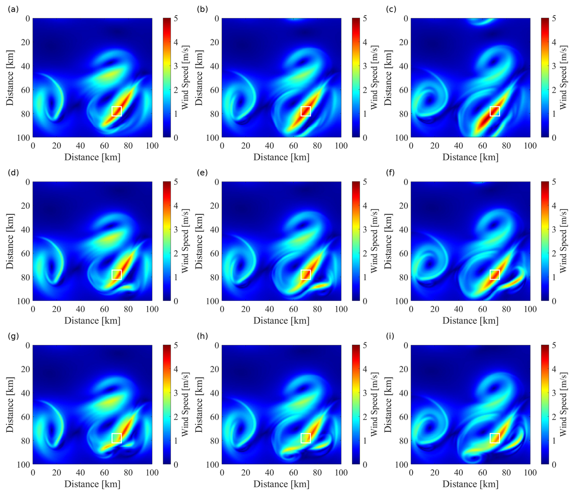
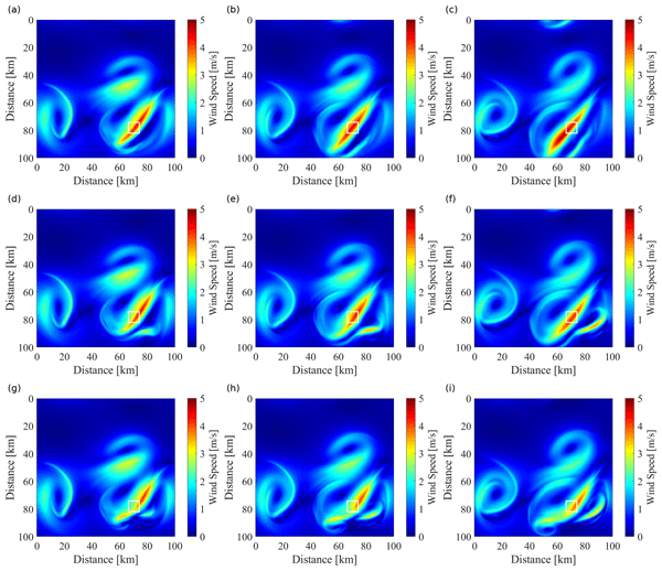
Figure 5 Wind-speed fields for the target region $[\mathrm{85},\mathrm{95}]\times [\mathrm{95},\mathrm{105}]$. Panels (a–c), (d–f), and (g–i) show the no-control, EnKC, and EKG-MPPI cases, respectively; the three columns correspond to days 4, 5, and 6. The white rectangle denotes the target region for wind-speed suppression.

The results are shown in Fig. 4. Focusing on the mean maximum wind speed and the mean intervention magnitude, we observe that EKG-MPPI achieves effective wind-speed suppression with smaller interventions in almost all scenarios. In particular, EKG-MPPI attains lower maximum wind speeds in the target region than EnKC (Fig. 4a), while requiring smaller mean control magnitudes (Fig. 4b). One reason why EKG-MPPI demonstrates superior control performance compared to EnKC is that EKG-MPPI leverages prior information provided by EnKC to perform MPPI with high sample efficiency, enabling the computation of control inputs that explicitly account for the nonlinear dynamics of the atmospheric system. On the other hand, the standard deviation of the intervention magnitude tends to be larger for EKG-MPPI. A possible reason is the additional exploration introduced by the sampling process in the MPPI component. In large-scale systems such as atmospheric dynamics, control performance is likely to vary significantly depending on the quality of the sampled intervention sequences, which can lead to larger variability in the required control effort. Another interesting observation is that the standard deviation of the maximum wind speed is particularly large in Scenarios 7 and 8. A possible reason is that, in these scenarios, it takes a relatively long time from the beginning of the simulation for the wind speed to intensify. As a result, the effects of interventions at each time step may accumulate over time, leading to more complex behavior of the atmospheric field.

For clarity, Fig. 5 shows visualizations of the no-control, EnKC, and EKG-MPPI simulations for the target region $[\mathrm{85},\mathrm{95}]\times [\mathrm{95},\mathrm{105}]$. Panels (a)–(c) show that strong winds occur in the target region in the absence of control. Panels (d)–(f) show that EnKC suppresses the wind speed relative to the no-control case, although localized regions of strong wind remain. Panels (g)–(i) show that EKG-MPPI achieves stronger wind-speed suppression in the target region than EnKC.

5 Conclusions

We developed EnKC-guided MPPI (EKG-MPPI), a hybrid control scheme that uses EnKC to obtain a sparse candidate perturbation and then refines it by MPPI using nonlinear forward rollouts. The EnKC output is used to shape the sampling distribution in MPPI, so that exploration is concentrated around plausible actuator locations and magnitudes instead of relying on uninformed sampling.

In the Lorenz-96 control simulation experiment, EKG-MPPI reduced the extreme-event count relative to EnKC while requiring a smaller input magnitude. Specifically, for X≥12, the extreme-event count decreased from 7820±142 for EnKC to 7622±146 for EKG-MPPI, while the input magnitude decreased from 0.191±0.001 to 0.166±0.002. In the SQG experiments over eight target regions, EKG-MPPI also achieved lower maximum wind speeds in the target region than EnKC, while using smaller mean control magnitudes.

The current implementation assumes localized actuation (a single or very sparse actuator) and applies the perturbation as a one-step input within each MPPI rollout, and it does not yet impose hard physical constraints. Future work will address multi-actuator and multi-step actuation, constraint-aware formulations, and evaluation metrics that explicitly quantify non-target impacts and robustness to model/observation uncertainty, in addition to improving computational efficiency for higher-dimensional models.

Appendix A: Standalone BO vs. vanilla MPPI

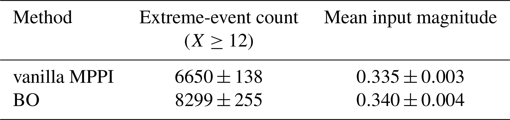
For completeness, we report here the comparison between standalone BO and vanilla MPPI in the same single-step Lorenz-96 setting as in Sect. 4.1.2. This appendix is included as a supplementary reference for the single-step setting. The parameter settings of vanilla MPPI are almost the same as those used for EKG-MPPI in Sect. 4.1.1. However, unlike EKG-MPPI, vanilla MPPI does not use EnKC-informed prior information for the intervention location or magnitude. Accordingly, the sampling distributions for the intervention location and intervention magnitude are fixed to 𝒩(0,20.0) and 𝒩(0,0.5), respectively. The parameter settings of BO are the same as those used in Sect. 4.1.2. As in Sect. 4.1.2, the experiments were repeated over 10 simulations with different random seeds, and we report the mean and standard deviation of each metric.

The results are summarized in Table A1. Vanilla MPPI yields fewer extreme events than standalone BO while requiring a comparable mean input magnitude. For reference, EKG-MPPI in Table 1 yields 7622±146 threshold exceedances with a mean input magnitude of 0.166±0.002, whereas vanilla MPPI yields 6650±138 threshold exceedances with a mean input magnitude of 0.335±0.003. Thus, in the present setting, vanilla MPPI achieves a lower threshold-exceedance count, whereas EKG-MPPI requires approximately half the mean control-input magnitude. These results indicate a trade-off between extreme-event suppression and control effort. Even without EnKC-informed guidance, vanilla MPPI therefore remains a competitive baseline in the present single-step setting.

Table A1 Comparison between vanilla MPPI and a standalone BO baseline in the single-step Lorenz-96 control setting. The second and third columns report the extreme-event count and the mean input magnitude, respectively, defined in the same manner as in Table 1. All values are shown as mean ± standard deviation over 10 simulations with different random seeds.

Appendix B: Rescaling used for visualization

To facilitate visual comparison in the two-dimensional performance–control plots, we rescale both the average intervention magnitude and the threshold-exceedance count (the horizontal-axis performance metric) by the corresponding mean over the five BO-MPPI runs for the same fixed value of λ. This rescaling is used only for visualization. Because each quantity is divided by a reference mean rather than mapped to the interval [0,1], we refer to the resulting quantities as rescaled (or mean-scaled) values rather than normalized values. All qualitative comparisons reported in the text are unchanged when the original, unscaled metrics are used. For each fixed λ, let $\mathcal{A}=\mathit{\{}\mathrm{100},\mathrm{10},\mathrm{1},\mathrm{0.1},\mathrm{0.01}\mathit{\}}$. Let m_EKG and m_α denote the average intervention magnitudes obtained by EKG-MPPI and BO-MPPI, respectively. We define the BO-MPPI reference mean by

$$\begin{array}{}\text{(B1)}& {\stackrel{\mathrm{‾}}{m}}_{\text{BO}}={\displaystyle \frac{\mathrm{1}}{\mathrm{5}}}\sum _{\mathit{\alpha }\in \mathcal{A}}{m}_{\mathit{\alpha }},\end{array}$$

and the corresponding rescaled quantities by

$$\begin{array}{}\text{(B2)}& {\stackrel{\mathrm{̃}}{m}}_{\text{EKG}}={\displaystyle \frac{m_{\text{EKG}}}{{\stackrel{\mathrm{‾}}{m}}_{\text{BO}}}},{\stackrel{\mathrm{̃}}{m}}_{\mathit{\alpha }}={\displaystyle \frac{m_{\mathit{\alpha }}}{{\stackrel{\mathrm{‾}}{m}}_{\text{BO}}}}.\end{array}$$

Similarly, let e_EKG and e_α denote the threshold-exceedance counts used on the horizontal axis. We define

$$\begin{array}{}\text{(B3)}& {\stackrel{\mathrm{‾}}{\mathit{e}}}_{\text{BO}}={\displaystyle \frac{\mathrm{1}}{\mathrm{5}}}\sum _{\mathit{\alpha }\in \mathcal{A}}{\mathit{e}}_{\mathit{\alpha }},\end{array}$$

and

$$\begin{array}{}\text{(B4)}& {\stackrel{\mathrm{̃}}{\mathit{e}}}_{\text{EKG}}={\displaystyle \frac{{\mathit{e}}_{\text{EKG}}}{{\stackrel{\mathrm{‾}}{\mathit{e}}}_{\text{BO}}}},{\stackrel{\mathrm{̃}}{\mathit{e}}}_{\mathit{\alpha }}={\displaystyle \frac{{\mathit{e}}_{\mathit{\alpha }}}{{\stackrel{\mathrm{‾}}{\mathit{e}}}_{\text{BO}}}}.\end{array}$$

Values below 1 therefore indicate performance better than the BO-MPPI mean for the same λ on the corresponding axis. Smaller horizontal values indicate fewer threshold exceedances, and smaller vertical values indicate a smaller average intervention magnitude. Since each axis is rescaled by a common positive constant within each panel, this transformation does not change the within-panel ordering or Pareto dominance relations; it only changes the axis units for visualization.