Noise-scaled accuracy of the ensemble Kalman filter with an instability-based minimum ensemble size

The ensemble Kalman filter (EnKF) is widely used for state estimation in chaotic dynamical systems, including atmospheric and oceanic flows. One of the fundamental questions is how many samples are required for accurate long-term performance of the EnKF. In this study, we introduce a notion of time-asymptotic filter accuracy based on the scaling of the analysis error with respect to the observation noise level. This formulation provides a qualitative distinction between convergent and divergent filtering behavior, beyond standard criteria based on time-averaged RMSE at a fixed noise level. We investigate the minimum ensemble size m^* required for this filter accuracy and relate it to intrinsic instability of dynamical systems. Using the Lyapunov exponents (LEs), which quantify asymptotic exponential growth rates of infinitesimal perturbations, we characterize degrees of instability by the number of positive exponents N₊. Because spanning the unstable directions by a limited ensemble is essential for long-term accuracy, we propose an ensemble spin-up and downsizing strategy. Numerical experiments with the EnKF applied to the Lorenz 96 model indicate that the minimum ensemble size required for this filter accuracy satisfies $m^{*}=N_{+}+\mathrm{1}$. These results provide a practical guideline for ensemble-size selection based on a priori dynamical information and bridge idealized theoretical requirements with feasible numerical implementations via the ensemble downsizing method.

1 Introduction

Many geophysical systems, including the motions of the atmosphere and ocean, are modeled as dissipative dynamical systems whose trajectories converge to compact attractors. These dynamics often exhibit chaotic behavior, characterized by sensitivity to initial conditions, which renders long-term forecasts unreliable (Kalnay, 2002). Therefore, quantifying the degree of instability in chaotic dynamics is essential. One approach to characterizing such instability is through tangent-linear approximations of dynamical systems, known as Lyapunov analysis. The degree of instability is quantified by the Lyapunov exponents (LEs), which characterize the asymptotic exponential rates of separation of nearby trajectories. These rates are defined through the evolution of infinitesimal perturbations governed by the linearized dynamics along a reference trajectory (Eckmann and Ruelle, 1985; Legras and Vautard, 1996). For autonomous continuous-time dynamical systems, such as autonomous ordinary differential equations, at least one of the LEs is zero, corresponding to perturbations parallel to the vector field (Haken, 1983). At each point on the attractor, the tangent space is decomposed into unstable, neutral, and stable subspaces, spanned by basis vectors with positive, zero, and negative exponential rates in the infinite time limit. We focus on the dimensions of these subspaces. The numbers of positive and non-negative LEs are denoted by N₊ and N₀, respectively. By definition, it follows that $N_{\mathrm{0}}\ge N_{+}$.

We consider Bayesian data assimilation for state estimation in chaotic dynamical systems, where noisy observations are obtained at discrete time steps. The ensemble Kalman filter (EnKF, Evensen, 2009) is widely used for this purpose. It estimates uncertainty in the forecast using an ensemble of state vectors and updates the mean and covariance via Bayes' rule. We focus on a deterministic version, the ensemble transform Kalman filter (ETKF, Bishop et al., 2001). The ensemble covariance, C_t, characterizes forecast uncertainty through its eigenpairs, with the eigenvalues quantifying the magnitude of variability and the eigenvectors specifying the principal directions along which this variability occurs. In the analysis step, corrections are applied more strongly in directions with higher forecast uncertainty. In general, the rank of the ensemble covariance C_t is less than the ensemble size m, i.e., $\mathrm{rank}\left({\mathbf{C}}_t\right)\le m-\mathrm{1}$. Moreover, in geophysical applications, m is limited because each ensemble member incurs a high computational cost. Therefore, it is crucial to estimate uncertain directions with a limited ensemble. If the ETKF underestimates an unstable direction, the state estimation error is not sufficiently corrected and grows to the size of the attractor. This phenomenon is known as filter divergence and must be avoided. To mitigate this problem, covariance inflation artificially increases the ensemble spread to compensate for underestimated uncertainty, thereby helping to prevent filter divergence. Note that inflation cannot remedy an insufficient ensemble size that fails to span the unstable directions. Another numerical technique is localization (Hamill et al., 2001; Hunt et al., 2007), which reduces the influence of distant observations by damping spurious long-range correlations in the ensemble covariance. Although localization can reduce the required ensemble size for practical applications, we do not consider it in order to isolate and analyze the relationship between ensemble size and the degrees of instability.

Mathematical studies of filtering algorithms often focus on the long-term accuracy (Kelly et al., 2014; Kelly and Stuart, 2019; Takeda and Sakajo, 2024; Biswas and Branicki, 2024; Sanz-Alonso and Waniorek, 2025). The central objective is to show that the squared error SE_t remains of order r² when the observation noise level r is sufficiently small compared with the attractor size, namely,

$$\begin{array}{}\text{(1)}& \lim {\sup }_{t\to \mathrm{\infty }}\mathbb{E}\left[{\mathrm{SE}}_t\right]=O\left(r^{\mathrm{2}}\right)\end{array}$$

for sufficiently small r, where the expectation is taken with respect to the probability distributions of the observation noise and the initial ensemble. We refer to this property as (r-asymptotic) filter accuracy. When we evaluate filter performance, compared with the standard RMSE-based criterion at a fixed noise level r, the present formulation based on Eq. (1) has the following notable features:

1. By Jensen’s inequality, the expectation of the SE dominates the squared expectation of the RMSE (up to a factor of the state dimension N_x), that is, 𝔼[SE_t]≥N_x(𝔼[RMSE_t])², which provides a stronger guarantee for filter performance.

2. The observation noise level r is treated as an asymptotic parameter, which facilitates rigorous mathematical analysis and enables a qualitative distinction between convergent and divergent filtering behavior based on the scaling with respect to r.

Takeda and Sakajo (2024) analyzed the ETKF for dissipative dynamical systems and proved filter accuracy under the large-ensemble condition $m\ge N_x+\mathrm{1}$, provided that sufficient inflation is applied. Since such an ensemble size is impractical in high-dimensional applications, a central question is whether filter accuracy can be achieved with a substantially smaller ensemble size determined by the intrinsic instability of the underlying dynamics.

Under more idealized assumptions, González-Tokman and Hunt (2013) investigated a lower bound on m for the ETKF. They proved that for discrete-time dynamical systems, if $m\ge N_{+}+\mathrm{1}$, the analysis error is bounded by the order of the observation noise. The proof relies on the following assumptions: the noise is sufficiently small; the initial ensemble is close to the true state and concentrated on the unstable subspace. Their analysis has two limitations: it applies only to discrete-time systems without zero LEs; the assumptions on the initial ensemble are not practically verifiable. Seminal studies (Trevisan and Uboldi, 2004; Trevisan et al., 2010; Trevisan and Palatella, 2011) investigated the use of the unstable subspace in data assimilation, known as Assimilation in Unstable Subspace (AUS). Related studies (Gurumoorthy et al., 2017; Bocquet et al., 2017; Bocquet and Carrassi, 2017; Grudzien et al., 2018a, b) analyzed the behavior of the (ensemble) Kalman filters and smoothers in relation to the unstable subspaces. These works mainly consider systems that include neutral directions and argue that correcting the state in the N₀-dimensional unstable-neutral subspace is crucial for filter performance. We now focus on results directly related to the ETKF. Theoretical analyses for linear systems have established that the forecast and analysis error covariance matrices of the EnKF asymptotically concentrate in the unstable-neutral subspace. In particular, Bocquet et al. (2017); Bocquet and Carrassi (2017) proved rigorously that, in the linear case, the error covariance matrix becomes asymptotically rank-deficient with rank at most N₀, and that an ensemble size of at least N₀+1 is required to properly represent the error covariance matrix. They also present numerical results by the ETKF for the Lorenz 96 model (Lorenz, 1996) with 40 variables. For instance, in Fig. 8 of Bocquet and Carrassi (2017), the time-averaged RMSE of the ETKF is shown as a function of the ensemble size m for the observation noise covariance matrix R=I. This figure shows that the RMSE is small relative to the observation noise level (∼ 1) when $m\ge N_{\mathrm{0}}+\mathrm{1}$, supporting the theoretical findings in Bocquet et al. (2017). Similar findings are reported in Bocquet (2011) for the same model and Carrassi et al. (2022) for the Quasi-Geostrophic model (Reinhold and Pierrehumbert, 1982) and the Modular Arbitrary-Order Ocean-Atmosphere Model (De Cruz et al., 2016). In these studies, the required ensemble size for accuracy can vary depending on the observation noise level, typically fixed to r=1.0.

The objective of this study is to clarify the relationship between the minimum ensemble size required for filter accuracy and the degrees of dynamical instability, under idealized conditions on the inflation factor and the observation noise level. Accordingly, we adopt a definition of filter accuracy based on its asymptotic behavior with respect to the observation noise level, as given in Eq. (1). Motivated by the studies reviewed above, and under the working assumption that the influence of neutral directions on filter accuracy becomes negligible in the joint long-time and small-noise limits, we revisit the conjecture that the minimum ensemble size for the r-asymptotic filter accuracy is given by

$$\begin{array}{}\text{(2)}& m^{*}=N_{+}+\mathrm{1}.\end{array}$$

In the numerical experiments presented in this study, we use dynamical systems with a single zero LE, so that $N_{\mathrm{0}}=N_{+}+\mathrm{1}$. More generally, it holds that $N_{+}+\mathrm{1}\le N_{\mathrm{0}}$ for continuous-time dynamical systems. Even in such cases, we still conjecture that the minimum ensemble size is $m^{*}=N_{+}+\mathrm{1}$. Therefore, we use N₊ rather than N₀ to represent the minimum ensemble size throughout the paper. To examine this conjecture within the formulation of the r-asymptotic filter accuracy, we conduct numerical experiments with the ETKF applied to the Lorenz 96 model with 40 variables. We estimate the minimum ensemble size m^* so that the asymptotic analysis error is bounded by the order of the observation noise when an appropriate multiplicative inflation factor is chosen. We then compare this value with the dimension of the unstable subspace N₊, computed via Lyapunov analysis. In our experiments, we also introduce an ensemble downsizing method for the ETKF: we begin with a sufficiently large ensemble size, $m=N_x+\mathrm{1}$, and reduce it to a smaller size after a fixed spin-up time. This procedure is intended to produce a small yet efficient ensemble, with its mean close to the true state and its perturbations aligned with the unstable subspace, thus approximately realizing the idealized initial conditions assumed in González-Tokman and Hunt (2013). Although the target model considered is the same as that in Bocquet and Carrassi (2017), our objective differs in that we focus on the reformulated minimum ensemble size based on the accuracy criterion as Eq. (1). Numerical investigations from this perspective are important because they define and qualitatively clarify the ensemble size below which filter divergence of the ETKF cannot be avoided, even when accurate observations and appropriate inflation are used. Moreover, establishing an error bound by order of the observation noise enables further mathematical analysis of the ETKF. Our approach is applicable when the LEs of the target dynamical system can be estimated, and it offers practical guidance for selecting ensemble size in high-dimensional ETKF applications.

Our main contributions are summarized as follows:

1. By adopting the reformulated r-asymptotic filter accuracy, we provide a qualitative criterion that distinguishes between divergent and accurate filtering behavior based on noise scaling, rather than relying on time-averaged RMSE at a fixed noise level.

2. We propose an ensemble spin-up and downsizing method that enables a practical realization of ensembles aligned with the unstable subspace, bridging idealized theoretical assumptions and feasible numerical implementations.

3. Through numerical experiments with the ETKF applied to the Lorenz 96 model, we provide evidence that the minimum ensemble size required for r-asymptotic filter accuracy scales with the number of unstable directions as $m^{*}=N_{+}+\mathrm{1}$, rather than N₀+1 with sufficiently small r or other observation conditions.

The remainder of the paper is organized as follows. In Sect. 2, we introduce the basics of Lyapunov analysis. In Sect. 3, we define the ETKF with the ensemble downsizing method. In Sect. 4, we present the numerical results with the Lorenz 96 model, combining Lyapunov analysis and the ETKF. In Sect. 5, we summarize our results and outline future directions.

2 Characterizing the degrees of instability in dynamics

2.1 The Lyapunov exponents and their computation

Let N_x∈ℕ. We consider the dynamics governed by

$$\begin{array}{}\text{(3)}& {\displaystyle \frac{\mathrm{d}}{\mathrm{d}t}}\mathit{x}\left(t\right)=\mathit{f}\left(\mathit{x}\right(t\left)\right),t>\mathrm{0}\end{array}$$

with $\mathit{x}\left(\mathrm{0}\right)={\mathit{x}}_{\mathrm{0}}\in {\mathbb{R}}^{N_x}$, where $\mathit{f}:{\mathbb{R}}^{N_x}\to {\mathbb{R}}^{N_x}$ is a smooth vector field. To study the instability of the dynamics, we examine the evolution of a perturbation $\mathit{\delta }\mathit{x}\left(t\right)\in {\mathbb{R}}^{N_x}$, defined as the difference between two trajectories separated by $\mathit{\delta }{\mathit{x}}_{\mathrm{0}}\in {\mathbb{R}}^{N_x}$ at t=0. Assuming that δx(t) is sufficiently small and smooth, its evolution is approximated by the linearization of Eq. (3):

$$\begin{array}{}\text{(4)}& {\displaystyle \frac{\mathrm{d}}{\mathrm{d}t}}\mathit{\delta }\mathit{x}\left(t\right)={\mathbf{J}}_{\mathit{f}}\left(\mathit{x}\right(t\left)\right)\mathit{\delta }\mathit{x}\left(t\right),t>\mathrm{0}\end{array}$$

with δx(0)=δx₀, where J_f(x(t)) denotes the Jacobian matrix of f at x=x(t). Equation (4) is referred to as the tangent linear model. Let $\mathbf{\Phi }(t,{\mathit{x}}_{\mathrm{0}})\in {\mathbb{R}}^{N_x\times N_x}$ denote the fundamental matrix solution to Eq. (4) with $\mathbf{\Phi }(\mathrm{0},{\mathit{x}}_{\mathrm{0}})={\mathbf{I}}_{N_x}$. The unique solution is then

$$\begin{array}{}\text{(5)}& \mathit{\delta }\mathit{x}\left(t\right)=\mathbf{\Phi }(t,{\mathit{x}}_{\mathrm{0}})\mathit{\delta }{\mathit{x}}_{\mathrm{0}},t\ge \mathrm{0}.\end{array}$$

The matrix Φ(t,x₀) encodes the deformation and amplification of infinitesimally small perturbations. For the singular values ${\mathit{\sigma }}_{\mathrm{1}}\left(\mathbf{\Phi }\right(t,{\mathit{x}}_{\mathrm{0}}\left)\right)\ge {\mathit{\sigma }}_{\mathrm{2}}\left(\mathbf{\Phi }\right(t,{\mathit{x}}_{\mathrm{0}}\left)\right)\ge \mathrm{\dots }\ge {\mathit{\sigma }}_{N_x}\left(\mathbf{\Phi }\right(t,{\mathit{x}}_{\mathrm{0}}\left)\right)>\mathrm{0}$ of Φ(t,x₀), we define

$$\begin{array}{}\text{(6)}& {\mathit{\lambda }}_j(t,{\mathit{x}}_{\mathrm{0}})={\displaystyle \frac{\mathrm{1}}{t}}\log {\mathit{\sigma }}_j\left(\mathbf{\Phi }\right(t,{\mathit{x}}_{\mathrm{0}}\left)\right)\in \mathbb{R},j=\mathrm{1},\mathrm{\dots },N_x.\end{array}$$

For each j, the singular vector ${\mathit{v}}_j\in {\mathbb{R}}^{N_x}$ associated with σ_j exponentially grows or decays at rate λ_j over [0,t] under the tangent linear model, i.e.,

$$\begin{array}{}\text{(7)}& \Vert \mathbf{\Phi }(t,{\mathit{x}}_{\mathrm{0}}){\mathit{v}}_j\Vert =e^{{\mathit{\lambda }}_{j}t}\Vert {\mathit{v}}_j\Vert ,\end{array}$$

where $\Vert \cdot \Vert$ is the Euclidean norm. Thus, the deformation of the initial perturbation δx₀ is expressed as exponential growth/decay along the directions v_j. Taking the limit t→∞, we obtain the asymptotic rates

$$\begin{array}{}\text{(8)}& {\mathit{\lambda }}_j\left({\mathit{x}}_{\mathrm{0}}\right)=\underset{t\to \mathrm{\infty }}{lim}{\mathit{\lambda }}_j(t,{\mathit{x}}_{\mathrm{0}})\in \mathbb{R},j=\mathrm{1},\mathrm{\dots },N_x,\end{array}$$

known as the Lyapunov exponents (LEs). The existence of these limits is guaranteed by Oseledets' Multiplicative Ergodic Theorem (Oseledets, 1968; Barreira and Pesin, 2002). If the dynamics Eq. (3) is ergodic, the LEs are uniquely determined regardless of the choice of x₀ belonging to an invariant subset of ${\mathbb{R}}^{N_x}$. For autonomous continuous-time dynamical systems of the form Eq. (3), at least one exponent is zero, λ_j=0, corresponding to a perturbation parallel to the vector field δx(t)=f(x(t)) (Haken, 1983). If the dynamics admits a positive exponent λ₁>0, there exists at least one unstable direction in which perturbations grow exponentially, i.e., the dynamics is chaotic. According to Sect. 1, we define the following dimension to quantify the degrees of freedom of unstable perturbations:

$$\begin{array}{}\text{(9)}& N_{+}=\mathit{\#}\mathit{\{}j\in \mathit{\{}\mathrm{1},\mathrm{\dots },N_x\mathit{\}}\mid {\mathit{\lambda }}_j>\mathrm{0}\mathit{\}}.\end{array}$$

See Legras and Vautard (1996) for a more comprehensive introduction to LEs and their associated vectors.

We estimate the LEs numerically using the standard algorithm based on QR decomposition, as detailed in Algorithm 1 (Sandri, 1996; von Bremen et al., 1997). To implement this algorithm, we require a vector field $\mathit{f}:{\mathbb{R}}^{N_x}\to {\mathbb{R}}^{N_x}$, its Jacobian ${\mathbf{J}}_{\mathit{f}}\in {\mathbb{R}}^{N_x\times N_x}$, an initial state ${\mathit{x}}_{\mathrm{0}}\in {\mathbb{R}}^{N_x}$, an ODE integrator IntegrateODE, a time step size Δt>0 and a number of iterations n∈ℕ. For the ODE integrator, we use the fourth-order Runge-Kutta method. The state x and the perturbations V are integrated together as an extended state S, where each is treated as a component of S; for example, S[2]=V.

Algorithm 1 Computing LEs using QR decomposition (Sandri, 1996; von Bremen et al., 1997).

Require:

f, J_f, x₀, IntegrateODE, Δt, n

Ensure:

$\mathbf{S}=(\mathit{x},\mathbf{V}),\mathbf{F}\left(\mathbf{S}\right)=\left(\mathit{f}\right(\mathit{x}),{\mathbf{J}}_{\mathit{f}}(\mathit{x}\left)\mathbf{V}\right)$

1:

$\mathbf{S}\leftarrow ({\mathit{x}}_{\mathrm{0}},{\mathbf{I}}_{N_x})$

2:

$LE\leftarrow \mathbf{0}\in {\mathbb{R}}^{N_x}$

3:

for i=1 to n do

4:

$\mathbf{S}\leftarrow \mathrm{IntegrateODE}(\mathbf{F},\mathbf{S},\mathrm{\Delta }t)$

5:

$\mathbf{Q},\mathbf{R}\leftarrow \mathrm{QR}\left(\mathbf{S}\right[\mathrm{2}\left]\right)$

6:

S[2]←Q

7:

$LE\leftarrow LE+\log \left(\right|\mathrm{diag}\left(\mathbf{R}\right)\left|\right)$

8:

end for

9:

return  $LE/\left(n\mathrm{\Delta }t\right)$

2.2 The Lorenz 96 model

For N_x∈ℕ number of variables, external forcing F∈ℝ and the state vector $\mathit{x}=(x^{\mathrm{1}},\mathrm{\dots },x^{N_x}{)}^{\top }\in {\mathbb{R}}^{N_x}$, the Lorenz 96 model (Lorenz, 1996) is given by

$$\begin{array}{}\text{(10)}& {\displaystyle \frac{\mathrm{d}{x}^i}{\mathrm{d}t}}=(x^{i+\mathrm{1}}-x^{i-\mathrm{2}})x^{i-\mathrm{1}}-x^i+F,i=\mathrm{1},\mathrm{\dots },N_x\end{array}$$

with $x^{-\mathrm{1}}=x^{N_x-\mathrm{1}}$, $x^{\mathrm{0}}=x^{N_x}$ and $x^{N_x+\mathrm{1}}=x^{\mathrm{1}}$. This is a spatio-temporal chaotic model on a one-dimensional periodic domain and often used in data assimilation algorithms. We use this model to show examples of chaotic dynamics with various degrees of instability by changing the parameter F.

3 The ensemble Kalman filter with the ensemble downsizing method

3.1 The filtering problem and the ensemble transform Kalman filter

We consider a discrete-time filtering problem for the dynamics Eq. (3) with noisy observations. Let t_n=nτ, $n=\mathrm{0},\mathrm{1},\mathrm{2},\mathrm{\dots }$, denote the observation times with a fixed interval τ>0. We define the flow map ${\mathbf{\Psi }}_{\mathit{\tau }}:{\mathbb{R}}^{N_x}\to {\mathbb{R}}^{N_x}$ such that Ψ_τ(x₀)=x(τ), where x(t) is the solution to Eq. (3) with x(0)=x₀. This yields the discrete-time dynamical system

$$\begin{array}{}\text{(11)}& {\mathit{x}}_n=\mathbf{\Psi }\left({\mathit{x}}_{n-\mathrm{1}}\right),n=\mathrm{1},\mathrm{2},\mathrm{\dots },\end{array}$$

where Ψ=Ψ_τ and x_n=x(t_n). The observations are obtained at each t_n as

$$\begin{array}{}\text{(12)}& {\mathit{y}}_n=\mathbf{H}{\mathit{x}}_n+{\mathit{\eta }}_n,n=\mathrm{1},\mathrm{2},\mathrm{\dots },\end{array}$$

where $\mathbf{H}\in {\mathbb{R}}^{N_y\times N_x}$ is the observation matrix, and ${\mathit{\eta }}_n\sim \mathcal{N}(\mathbf{0},\mathbf{R})$ is a Gaussian observation noise with a symmetric positive definite covariance matrix $\mathbf{R}\in {\mathbb{R}}^{N_y\times N_y}$. To estimate the state x_n from the observations $\mathit{\{}{\mathit{y}}_{\mathrm{1}},\mathrm{\dots },{\mathit{y}}_n\mathit{\}}$, we employ the ensemble Kalman filter (EnKF, Evensen, 2009), which approximates the mean and covariance of the filtering distribution with an ensemble of state vectors. The EnKF consists of the forecast and analysis steps. In the forecast step, each ensemble member evolves according to the model dynamics as

$$\begin{array}{}\text{(13)}& {\mathit{x}}_n^{\mathrm{f}\left(k\right)}=\mathbf{\Psi }\left({\mathit{x}}_{n-\mathrm{1}}^{\mathrm{a}\left(k\right)}\right),k=\mathrm{1},\mathrm{\dots },m,\end{array}$$

where m∈ℕ is the ensemble size, and the superscripts f and a denote forecast and analysis, respectively. In the analysis step, the ensemble is updated using Bayes' rule restricted to the Gaussian setting. We employ a particular analysis scheme called the ensemble transform Kalman filter (ETKF, Bishop et al., 2001). The ETKF updates the mean and perturbation part of the ensemble as

$$\begin{array}{}\text{(14)}& {\displaystyle }{\stackrel{\mathrm{‾}}{\mathit{x}}}_n^{\mathrm{a}}={\stackrel{\mathrm{‾}}{\mathit{x}}}_n^{\mathrm{f}}+{\mathbf{K}}_n\left({\mathit{y}}_n-\mathbf{H}{\stackrel{\mathrm{‾}}{\mathit{x}}}_n^{\mathrm{f}}\right),\text{(15)}& {\displaystyle }{\mathbf{V}}_n^{\mathrm{a}}={\mathbf{V}}_n^{\mathrm{f}}{\mathbf{T}}_n,\end{array}$$

where ${\stackrel{\mathrm{‾}}{\mathit{x}}}_n^{\mathrm{f}}=\frac{\mathrm{1}}{m}{\sum }_{k=\mathrm{1}}^m{\mathit{x}}_n^{\mathrm{f}\left(k\right)}$, ${\mathbf{V}}_n^{\mathrm{f}}=[{\mathit{x}}_n^{f\left(\mathrm{1}\right)}-{\stackrel{\mathrm{‾}}{\mathit{x}}}_n^{\mathrm{f}},\mathrm{\dots },{\mathit{x}}_n^{f\left(m\right)}-{\stackrel{\mathrm{‾}}{\mathit{x}}}_n^{\mathrm{f}}]\in {\mathbb{R}}^{N_x\times m}$, ${\mathbf{K}}_n={\mathbf{C}}_n^{\mathrm{f}}{\mathbf{H}}^{\top }({\mathbf{HC}}_n^{\mathrm{f}}{\mathbf{H}}^{\top }+\mathbf{R}{)}^{-\mathrm{1}}$ is the Kalman gain, ${\mathbf{C}}_n^{\mathrm{f}}={\mathbf{V}}_n^{\mathrm{f}}({\mathbf{V}}_n^{\mathrm{f}}{)}^{\top }/(m-\mathrm{1})$ is the forecast covariance, and ${\mathbf{T}}_n\in {\mathbb{R}}^{m\times m}$ is a transform matrix defined as

$$\begin{array}{}\text{(16)}& {\mathbf{T}}_n={\left({\mathbf{I}}_m+{\displaystyle \frac{\mathrm{1}}{m-\mathrm{1}}}({\mathbf{V}}_n^{\mathrm{f}}{)}^{\top }{\mathbf{H}}^{\top }{\mathbf{R}}^{-\mathrm{1}}{\mathbf{HV}}_n^{\mathrm{f}}\right)}^{-\mathrm{1}/\mathrm{2}},\end{array}$$

where the matrix square root is chosen to be symmetric positive definite. Finally, the analysis ensemble members are reconstructed as

$$\begin{array}{}\text{(17)}& {\mathit{x}}_n^{\mathrm{a}\left(k\right)}={\stackrel{\mathrm{‾}}{\mathit{x}}}_n^{\mathrm{a}}+{\mathit{v}}_n^{\mathrm{a}\left(k\right)},k=\mathrm{1},\mathrm{\dots },m,\end{array}$$

where ${\mathit{v}}_n^{\mathrm{a}\left(k\right)}$ denotes the kth column of ${\mathbf{V}}_n^{\mathrm{a}}$.

As mentioned in Sect. 1, the forecast ensemble is corrected more strongly in directions with higher uncertainty, as represented by the forecast covariance ${\mathbf{C}}_n^{\mathrm{f}}$. However, the rank of ${\mathbf{C}}_n^{\mathrm{f}}$ is at most m−1 with m ensemble members. As well as this rank deficiency, the ensemble covariance suffers from the underestimation of variance due to the limited ensemble size. To mitigate these issues, we employ multiplicative covariance inflation:

$$\begin{array}{}\text{(18)}& {\mathbf{V}}_n^{\mathrm{f}}\leftarrow \mathit{\alpha }{\mathbf{V}}_n^{\mathrm{f}},\end{array}$$

where α≥1 is the inflation factor.

To evaluate the long-term performance of the filter along the context of rigorous error analysis (Kelly et al., 2014; Kelly and Stuart, 2019; Takeda and Sakajo, 2024; Biswas and Branicki, 2024; Sanz-Alonso and Waniorek, 2025), we define filter accuracy as follows. Assume $\mathbf{R}=r^{\mathrm{2}}{\mathbf{I}}_{N_y}$ with r>0. The EnKF achieves filter accuracy if there exists a constant c>0, independent of r, such that

$$\begin{array}{}\text{(19)}& \lim {\sup }_{n\to \mathrm{\infty }}\mathbb{E}\left[{\mathrm{SE}}_n\right]=\lim {\sup }_{n\to \mathrm{\infty }}\mathbb{E}[\Vert {\mathit{x}}_n-{\stackrel{\mathrm{‾}}{\mathit{x}}}_n^{\mathrm{a}}{\Vert }^{\mathrm{2}}]\le c{r}^{\mathrm{2}}\end{array}$$

for sufficiently small r, where the expectation is taken with respect to the probability distributions of the observation noise and the initial ensemble. We reformulate the minimum ensemble size m^* for the ETKF based on this definition of filter accuracy as the smallest m∈ℕ such that the ETKF achieves filter accuracy Eq. (19) with an appropriate choice of the inflation factor α>1. As explained in Sect. 1, this formulation differs from the standard criterion using the RMSE with a fixed r in two aspects. First, the filter accuracy in Eq. (19) implies that the time-average of the expectation of RMSE is the order of r. But, the converse is not necessarily true due to Jensen's convex inequality. Thus, Eq. (19) provides a stronger guarantee for filter performance than the standard criterion (see Appendix A for more details). Second, the observation noise level r is treated as an asymptotic parameter, which makes rigorous mathematical analysis easier and qualitatively distinguishes between divergent and accurate filtering behavior using the dependency on r. Owing to this formulation, we can clearly define the minimum ensemble size m^* and simplify the analysis of its relationship with the geometric properties of the instability of dynamics.

3.2 The ensemble downsizing method

To generate an ensemble with its mean close to the true state and its perturbations aligned with the unstable subspace, we introduce an ensemble downsizing method. We begin with a sufficiently large ensemble size, m₀, and reduce it to a smaller size, m, at a fixed spin-up time, n=N_spinup. We call the period before n=N_spinup the ensemble spin-up period. In the ensemble downsizing method, we apply the singular value decomposition (SVD) to the ensemble perturbation, $\mathbf{V}\in {\mathbb{R}}^{N_x\times m_{\mathrm{0}}}$, and retain only the leading m modes. This procedure is detailed in Algorithm 2. We suppose that the SVD algorithm returns the singular values in decreasing order and the associated singular vectors accordingly. For a matrix A, we use MATLAB-style indexing notation: $\mathbf{A}[:,\mathrm{1}:m]$ denotes the submatrix formed by the first m columns of A, and $\mathbf{A}[\mathrm{1}:m,\mathrm{1}:m]$ denotes the leading m×m principal submatrix.

Algorithm 2 The ensemble downsizing method by the singular value decomposition.

Require:

$\mathbf{X}\in {\mathbb{R}}^{N_x\times m_{\mathrm{0}}}$, m<m₀

Ensure:

$\mathbf{X}=\stackrel{\mathrm{‾}}{\mathit{x}}+\mathbf{V}$

1:

$\mathbf{U},\mathbf{\Sigma },\mathit{\_}\leftarrow \mathrm{SVD}\left(\mathbf{V}\right)$

2:

$\mathbf{V}\leftarrow \mathbf{U}[:,\mathrm{1}:m]\mathbf{\Sigma }[\mathrm{1}:m,\mathrm{1}:m]$

3:

return  $\stackrel{\mathrm{‾}}{\mathit{x}}+\mathbf{V}$

The resulting ETKF with the multiplicative covariance inflation Eq. (18) and the ensemble downsizing method is summarized in Algorithm 3.

Algorithm 3 The ETKF with multiplicative covariance inflation and ensemble downsizing.

Require:

Ψ, H, R, $({\mathit{y}}_n{)}_{n=\mathrm{1}}^N$, ${\mathbf{X}}_{\mathrm{0}}\in {\mathbb{R}}^{N_x\times m_{\mathrm{0}}}$, α>1, N_spinup<N, m<m₀

Ensure:

$\mathbf{X}=({\mathit{x}}^{\left(k\right)}{)}_{k=\mathrm{1}}^{m^{\prime }}$

1:

X←X₀

2:

$m^{\prime }\leftarrow m_{\mathrm{0}}$

3:

for n=1 to N do

4:

# Forecast step

5:

for k=1 to m^′ do

6:

x^f(k)←Ψ(x^a(k))

7:

end for

8:

${\stackrel{\mathrm{‾}}{\mathit{x}}}^{\mathrm{f}}\leftarrow \frac{\mathrm{1}}{m^{\prime }}{\sum }_{k=\mathrm{1}}^{m^{\prime }}{\mathit{x}}^{\mathrm{f}\left(k\right)}$

9:

${\mathbf{V}}^{\mathrm{f}}\leftarrow [{\mathit{x}}^{f\left(\mathrm{1}\right)}-{\stackrel{\mathrm{‾}}{\mathit{x}}}^{\mathrm{f}},\mathrm{\dots },{\mathit{x}}^{f\left(m^{\prime }\right)}-{\stackrel{\mathrm{‾}}{\mathit{x}}}^{\mathrm{f}}]$

10:

# Covariance inflation

11:

V^f←α V^f

12:

${\mathbf{C}}^{\mathrm{f}}\leftarrow {\mathbf{V}}^{\mathrm{f}}({\mathbf{V}}^{\mathrm{f}}{)}^{\top }/(m^{\prime }-\mathrm{1})$

13:

# Analysis step

14:

$\mathbf{K}\leftarrow {\mathbf{C}}^{\mathrm{f}}{\mathbf{H}}^{\top }({\mathbf{HC}}^{\mathrm{f}}{\mathbf{H}}^{\top }+\mathbf{R}{)}^{-\mathrm{1}}$

15:

${\stackrel{\mathrm{‾}}{\mathit{x}}}^{\mathrm{a}}\leftarrow {\stackrel{\mathrm{‾}}{\mathit{x}}}^{\mathrm{f}}+\mathbf{K}({\mathit{y}}_n-\mathbf{H}{\stackrel{\mathrm{‾}}{\mathit{x}}}^{\mathrm{f}})$

16:

$\mathbf{T}\leftarrow ({\mathbf{I}}_{m^{\prime }}+\frac{\mathrm{1}}{m^{\prime }-\mathrm{1}}({\mathbf{V}}^{\mathrm{f}}{)}^{\top }{\mathbf{H}}^{\top }{\mathbf{R}}^{-\mathrm{1}}{\mathbf{HV}}^{\mathrm{f}}{)}^{-\mathrm{1}/\mathrm{2}}$

17:

V^a←V^fT

18:

$\mathbf{X}\leftarrow {\stackrel{\mathrm{‾}}{\mathit{x}}}^{\mathrm{a}}+{\mathbf{V}}^{\mathrm{a}}$

19:

X_n←X

20:

# Ensemble downsizing

21:

if n=N_spinup then

22:

$\mathbf{X}\leftarrow \mathrm{EnsembleDownsizing}(\mathbf{X},m)$

23:

$m^{\prime }\leftarrow m$

24:

end if

25:

end for

26:

return  $({\mathbf{X}}_n{)}_{n=\mathrm{1}}^N$

See Tippett et al. (2003) for an efficient implementation of the analysis step.

4 Numerical results

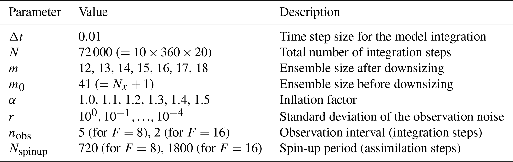
To verify our conjecture that the minimum ensemble size for filter accuracy of the ETKF based on Eq. (19) is $m^{*}=N_{+}+\mathrm{1}$, we perform numerical experiments with the Lorenz 96 model. Throughout this section, we set N_x=40, $\mathbf{H}={\mathbf{I}}_{N_x}$ and $\mathbf{R}=r^{\mathrm{2}}{\mathbf{I}}_{N_x}$, where r>0 is a parameter representing the standard deviation of the observation noise. We consider two settings for the external forcing: F=8, 16. For each setting, we compute the LEs and estimate N₊ using Algorithm 1. Then, we apply the ETKF with the ensemble downsizing method (Algorithm 3) to the Lorenz 96 model. We summarize the common parameters for the ETKF experiments in Table 1. The initial ensemble X₀ is defined as ${\mathbf{X}}_{\mathrm{0}}=({\mathit{x}}_{\mathrm{0}}^{\left(k\right)}{)}_{k=\mathrm{1}}^{m_{\mathrm{0}}}$ with ${\mathit{x}}_{\mathrm{0}}^{\left(k\right)}\sim \mathcal{N}({\mathit{x}}_{\mathrm{0}},\mathrm{25}{\mathbf{I}}_{N_x})$, where ${\mathit{x}}_{\mathrm{0}}\in {\mathbb{R}}^{N_x}$ is uniformly sampled from the true trajectory.

Table 1 Common parameters for the ETKF experiments.

To evaluate the filter accuracy of the ETKF, we use the SE as in Eq. (19). To approximate the expectation 𝔼, we compute parallel simulations for n_seeds random seeds to generate the observation noises. Then, we take the maximum after n=N_∞ to approximate lim sup_n→∞. This procedure leads to

$$\begin{array}{}\text{(20)}& \begin{array}{rl}\lim {\sup }_{n\to \mathrm{\infty }}& \mathbb{E}[\Vert {\mathit{x}}_n-{\stackrel{\mathrm{‾}}{\mathit{x}}}_n^{\mathrm{a}}{\Vert }^{\mathrm{2}}]\approx \underset{n\ge N_{\mathrm{\infty }}}{max}{\displaystyle \frac{\mathrm{1}}{n_{\mathrm{seeds}}}}\\ & \sum _{i=\mathrm{1}}^{n_{\mathrm{seeds}}}\Vert {\mathit{x}}_n-{\stackrel{\mathrm{‾}}{\mathit{x}}}_n^{\mathrm{a}}\left({\mathit{\omega }}_i\right){\Vert }^{\mathrm{2}},\end{array}\end{array}$$

where ${\stackrel{\mathrm{‾}}{\mathit{x}}}_n^{\mathrm{a}}\left({\mathit{\omega }}_i\right)$ is the analysis mean of a sample path with the ith random seed. We use $N_{\mathrm{\infty }}=N/\mathrm{2}$ and n_seeds=10 to compute Eq. (20). On the other hand, we use the RMSE to visualize the time series of the analysis error for a sample run.

4.1  F=8

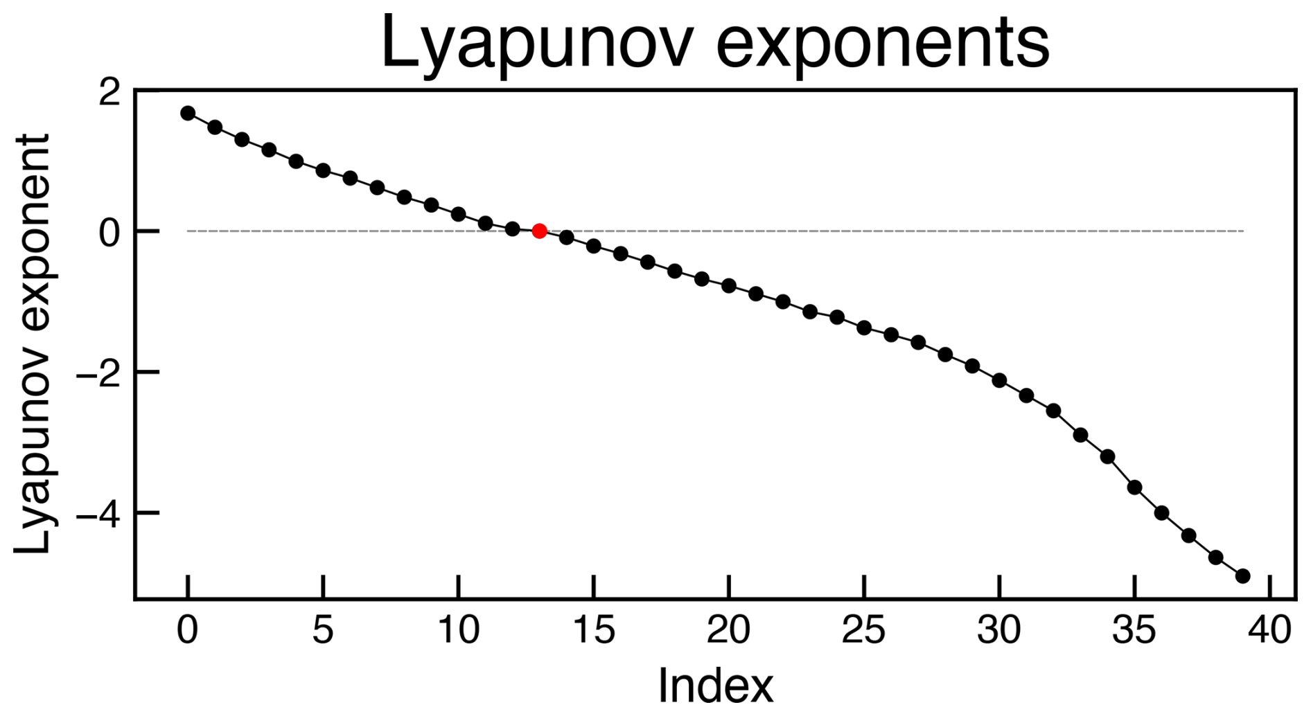
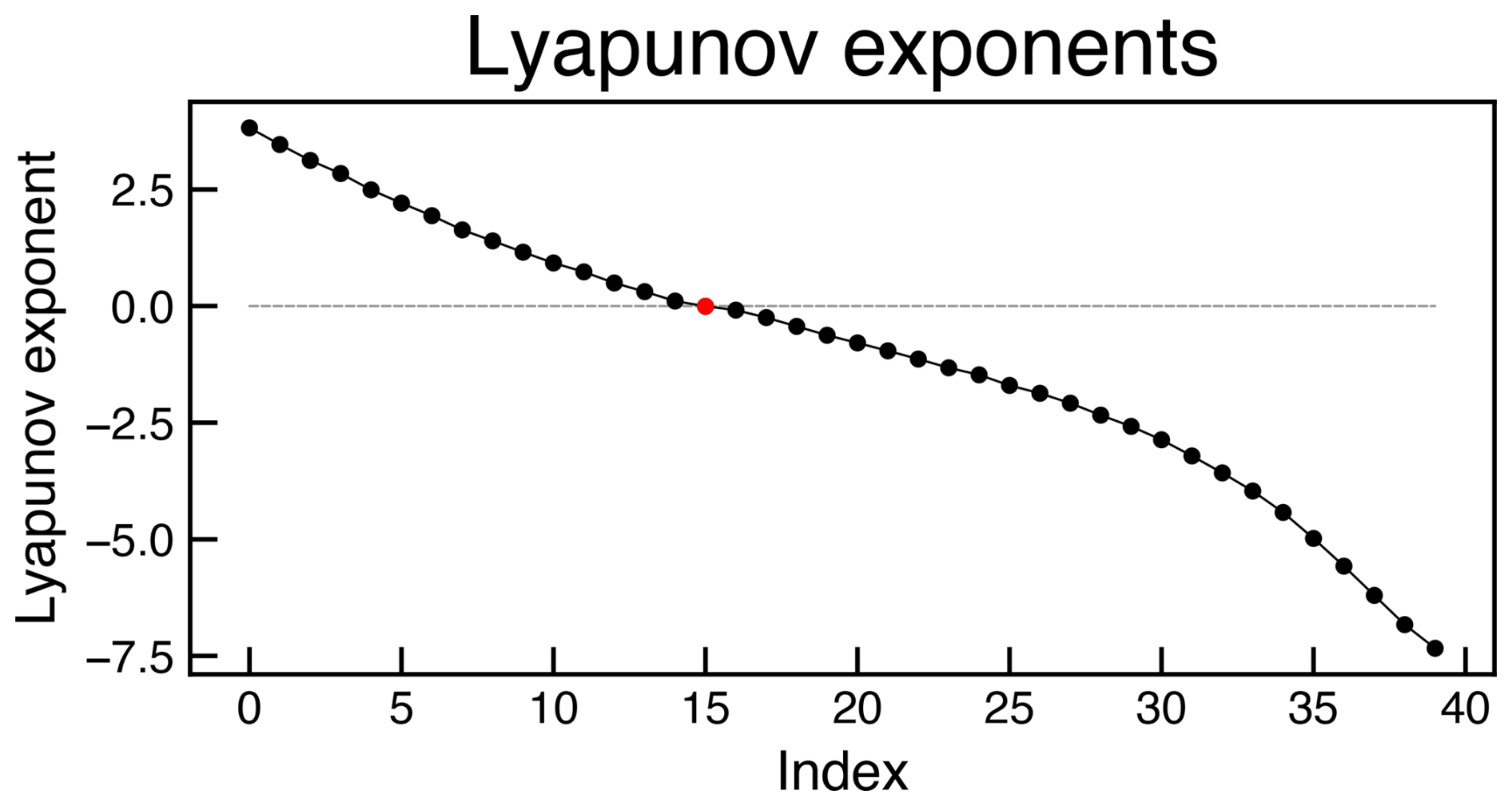
We first set F=8, a typical parameter for which the Lorenz 96 model exhibits chaotic behavior. The LEs are computed using Algorithm 1 with Δt=0.001 and n=10⁶ (Fig. 1). In the computation, we define the index of the zero exponent as the minimizer of $i\to \left|{\mathit{\lambda }}_i\right|$. This yields $N_{+}=\mathrm{13}$ and the largest LE λ₁≈1.67.

Figure 1 The LEs of the Lorenz 96 model with $(J,F)=(\mathrm{40},\mathrm{8})$. The zero exponent λ₁₄=0 is indicated in red.

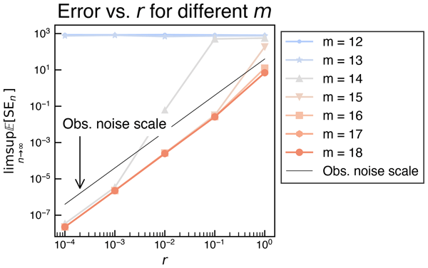
In this section, we set the observation time interval 0.05 (i.e., n_obs=5). We reduce the ensemble size after N_spinup=720 assimilation steps. For each pair (r,m), we vary the inflation factor α to find the optimal value that minimizes the SE defined in Eq. (20). The results are shown in Fig. 2 with log-log plots of the SE against r for different m. If m is larger than or equal to $N_{+}+\mathrm{1}=\mathrm{14}$, the SE is bounded by the order of r², indicating that the ETKF achieves filter accuracy. Conversely, if m is smaller than 14, the SE stays around O(1) even for small r, indicating that the ETKF does not achieve filter accuracy. Accordingly, our formulation of the filter accuracy Eq. (19) qualitatively distinguishes between divergent and accurate filtering behavior and evaluates the minimum ensemble size as $m^{*}=N_{+}+\mathrm{1}=\mathrm{14}$ in this setting. In particular, in the border case m=14, the ensemble spin-up works effectively under the small r assumption because the SE is larger than the order of r² for relatively large r but becomes comparable to it for small r. To allow for a relaxed condition of using large r with m=14, we examine an alternative condition, a short time interval, for practical settings with fixed r in Appendix B.

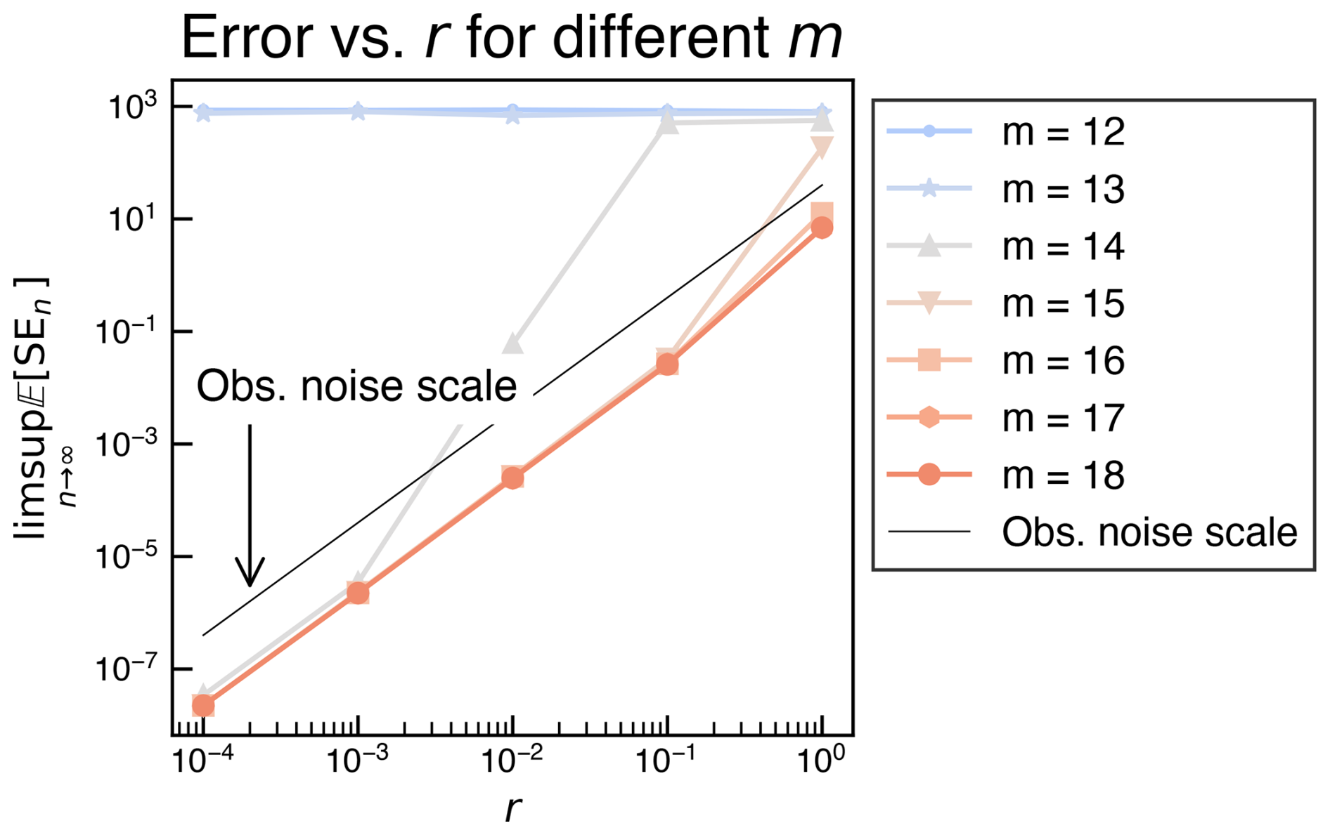
Figure 2 Log-log plots of the SE vs. r for different ensemble sizes m after the downsizing. The black line indicates the order of r², corresponding to the observation noise scale. The Lorenz 96 model with F=8 ($N_{+}=\mathrm{13}$) is used.

We then conduct a longer experiment (N=720 000) to investigate the dependence of the RMSE on the spin-up period N_spinup with a single random seed to generate the observation noise. We set $r={\mathrm{10}}^{-\mathrm{4}}$ and m=14, which avoids filter divergence in the experiment for Fig. 2. For N_spinup=0 and 720, we show the time series of the RMSE with various α in Fig. 3. In Fig. 3a, all series of the RMSE quickly decay to values with the order of r. Moreover, the filter remains stable over a long assimilation period. In Fig. 3b, the RMSE with α=1.5 decays to a small value. The time required for the RMSE to decay is much longer than that in Fig. 3a. A potential explanation for this phenomenon is the slow decay of the uncertainty in the neutral direction. Since we focus on the time asymptotic accuracy, this phenomenon is not further investigated in this study. From these results, we conclude that the ensemble spin-up and downsizing method effectively saves the computational time to generate a small ensemble sustaining filter accuracy, which is crucial in more high-dimensional applications.

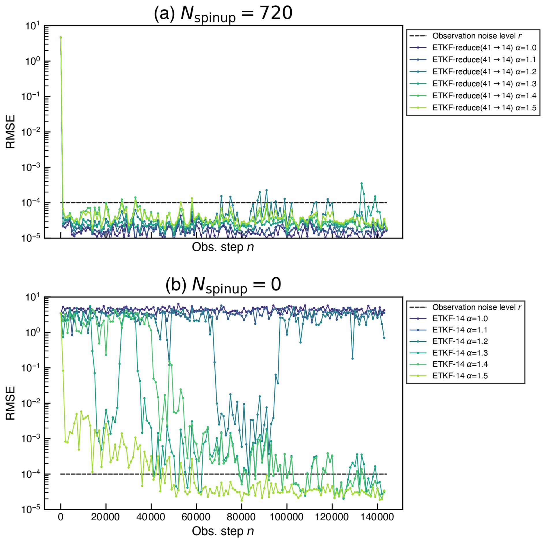
Figure 3 The time series of the RMSE with $r={\mathrm{10}}^{-\mathrm{4}}$, m=14 and various $\mathit{\alpha }=\mathrm{1.0},\mathrm{\dots },\mathrm{1.5}$ for (a) N_spinup=720 and (b) N_spinup=0. The dashed line indicates the level r.

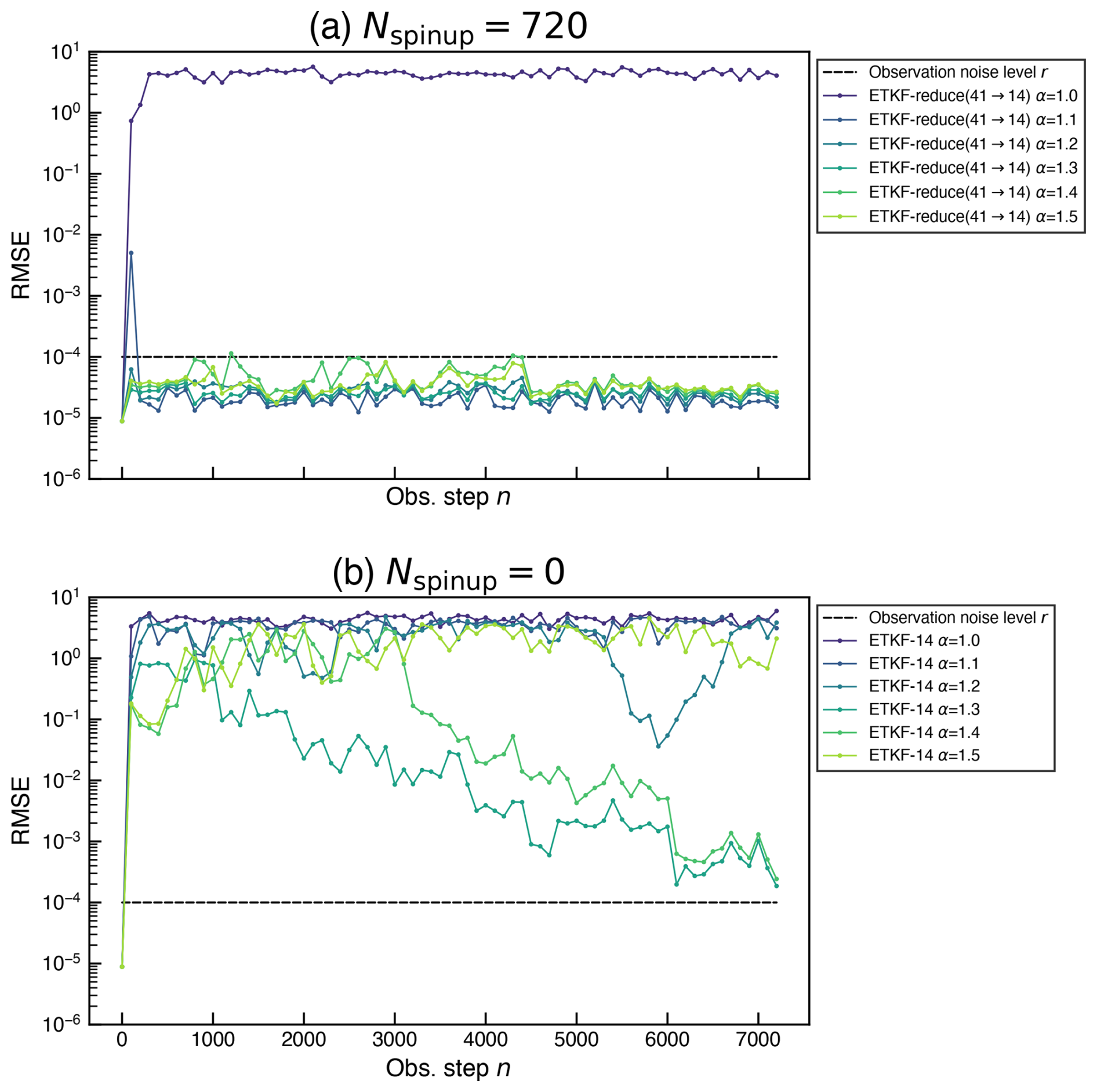
We then investigate the effect of the ensemble spin-up on the ensemble alignment with the unstable subspace. The integration time is N=360 000 and a single random seed is used to generate the observation noise. To clarify the effect of the ensemble downsizing method related to the unstable subspace, we perform experiments with initial ensemble which has accurate mean close to the true state and inaccurate perturbations not aligned in the unstable subspace. Specifically, the initial ensemble ${\mathbf{X}}_{\mathrm{0}}\in {\mathbb{R}}^{N_x\times m}$ is generated as

$$\begin{array}{}\text{(21)}& \begin{array}{rl}{\mathbf{X}}_{\mathrm{0}}& =[{\stackrel{\mathrm{‾}}{\mathit{x}}}_{\mathrm{0}}+{\mathit{v}}_{\mathrm{0}}^{\left(k\right)}{]}_{k=\mathrm{1}}^m,{\stackrel{\mathrm{‾}}{\mathit{x}}}_{\mathrm{0}}\sim \mathcal{N}({\mathit{x}}_{\mathrm{0}},\mathrm{0.01}\mathbf{R}),\\ & {\mathit{v}}_{\mathrm{0}}^{\left(k\right)}\sim \mathcal{N}(\mathbf{0},\mathrm{0.01}\mathbf{R})\end{array}\end{array}$$

for some m∈ℕ. This construction yields that the expected initial RMSE is the order of 0.1r, but the alignment of the ensemble perturbations with the unstable subspace is not guaranteed. Figure 4 shows the time series of the RMSE with $r={\mathrm{10}}^{-\mathrm{4}}$, m=14, various $\mathit{\alpha }=\mathrm{1.0},\mathrm{\dots },\mathrm{1.5}$ for (a) N_spinup=720 and (b) N_spinup=0. While the RMSE with the ensemble spin-up and downsizing method in Fig. 4a sustains the order of r for almost all α, the RMSE without the ensemble spin-up immediately diverges for all α and then decays very slowly for only some α. These results distinguish the ETKF with the ensemble spin-up and downsizing method from the one without it in terms of sustaining filter accuracy with inaccurate initial perturbations not aligned with the unstable subspace. To capture the unstable subspace of nonlinear dynamical systems, accurate state estimation is necessary but not sufficient since the unstable subspace depends on the state. The result in Fig. 4 implies that the ensemble spin-up method can assist not only the convergence of the ensemble mean to the true state but also the alignment of the ensemble perturbations with the unstable subspace.

Figure 4 The time series of the RMSE with $r={\mathrm{10}}^{-\mathrm{4}}$, m=14, various $\mathit{\alpha }=\mathrm{1.0},\mathrm{\dots },\mathrm{1.5}$ for (a) N_spinup=720 and (b) N_spinup=0. The accurate initial ensemble is given by Eq. (21). The dashed line indicates the level r.

4.2  F=16

To verify that $m^{*}=N_{+}+\mathrm{1}$ also holds with different value of N₊, we set F=16 and compute the LEs as in the previous section, shown in Fig. 5. This yields $N_{+}=\mathrm{15}$ and the largest LE λ₁≈3.82.

Figure 5 The LEs of the Lorenz 96 model with $(J,F)=(\mathrm{40},\mathrm{16})$. The zero exponent λ₁₆=0 is indicated in red.

We set the observation time interval 0.02 (i.e., n_obs=2) in this section. Since we control the interval using n_obs in the experiments, the value is determined by the largest integer n_obs with which the approximated error expansion n_obsλ₁Δt in the forecast step for F=16 does not exceed that with n_obs=5 for F=8. Indeed, if we write these quantities for F as $n_{\mathrm{obs}}^{\left(F\right)}$ and ${\mathit{\lambda }}_{\mathrm{1}}^{\left(F\right)}$, the error expansion with each F is approximated as

$$\begin{array}{c}{\displaystyle }{n}_{\mathrm{obs}}^{\left(\mathrm{8}\right)}{\mathit{\lambda }}_{\mathrm{1}}^{\left(\mathrm{8}\right)}\mathrm{\Delta }t\approx \mathrm{5}\cdot \mathrm{1.67}\cdot \mathrm{0.01}=\mathrm{8.35},\\ {\displaystyle }{n}_{\mathrm{obs}}^{\left(\mathrm{16}\right)}{\mathit{\lambda }}_{\mathrm{1}}^{\left(\mathrm{16}\right)}\mathrm{\Delta }t\approx \mathrm{2}\cdot \mathrm{3.82}\cdot \mathrm{0.01}=\mathrm{7.64}.\end{array}$$

We compute the SE in the same manner as in the previous section with N=72 000 integration steps and N_spinup=1800 assimilation steps, which yields the same integration steps before the ensemble downsizing method. The dependence of the SE on r for different m is shown in Fig. 6. As in the previous section, $m\ge N_{+}+\mathrm{1}=\mathrm{16}$ gives filter accuracy, while m<16 does not. Therefore, the minimum ensemble size for filter accuracy is $m^{*}=N_{+}+\mathrm{1}=\mathrm{16}$.

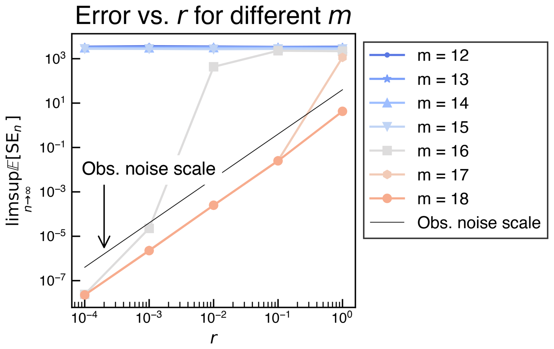
Figure 6 Log-log plots of the SE vs. r for different ensemble sizes m after the downsizing. The black line indicates the order of r², corresponding to the observation noise scale. The Lorenz 96 model with F=16 ($N_{+}=\mathrm{15}$) is used.

5 Conclusions

We reformulated the minimum ensemble size for filter accuracy of the EnKF based on the r-asymptotic filter accuracy Eq. (19), and investigated its relationship with the instability of dynamics characterized by the LEs. To obtain the effective small ensemble sustaining the filter accuracy, we proposed the ensemble spin-up and downsizing method for the EnKF generating an ensemble aligned with the unstable subspace of the dynamics. Through numerical experiments with the ETKF applied to the Lorenz 96 model, we verified our conjecture that the minimum ensemble size for the filter accuracy is $m^{*}=N_{+}+\mathrm{1}$, where N₊ is the number of positive LEs (Figs. 1, 5). In particular, our formulation qualitatively distinguishes between divergent and accurate filtering behavior through the observation noise scaling. This estimate of m^* is valid for the multiple external forcing F in the Lorenz 96 model (Figs. 2 and 6), and the filter remains stable over long assimilation periods (Fig. 3). Even without an ensemble spin-up period, the filter accuracy is achieved (Fig. 3). The ensemble downsizing method has an advantage in the border case $m=m^{*}$ as the error decays quickly with it while the error decays very slowly without it, which is a practical advantage of this method. Since our results depend on the choice of the inflation factor, we recommend employing an adaptive inflation scheme such as the EnKF-N (Bocquet, 2011) to avoid manual tuning.

In this study, the estimate of the minimum ensemble size $m^{*}=N_{+}+\mathrm{1}$ has been verified only for systems with a single zero LE. In general, there may exist multiple zero LEs, which can lead to a larger difference between N₊ and N₀. Further studies are needed to verify whether the estimate $m^{*}=N_{+}+\mathrm{1}$ holds in such cases. Suitable dynamical systems for this purpose include Hamiltonian systems with multiple zero LEs or the Modular Arbitrary-Order Ocean-Atmosphere Model (De Cruz et al., 2016) which exhibits many negative LEs close to zero as discussed in (Carrassi et al., 2022). Additionally, an explicit quantitative analysis of the alignment between ensemble covariance eigenvectors and Lyapunov vectors is an important topic, left for future work. This analysis will clarify the mechanism of the ensemble alignment within the spin-up period and enhance the validity of the ensemble downsizing method. The other future direction is to evaluate the minimum ensemble size with localization, in which we need to define “local degrees of instability” associated with a localization radius.

Appendix A: Comparison of error evaluation criteria

Mathematical studies for filters often focus on the long-term behavior of the analysis error (Kelly et al., 2014; Kelly and Stuart, 2019; Takeda and Sakajo, 2024; Biswas and Branicki, 2024; Sanz-Alonso and Waniorek, 2025) and aim to establish the bound known as time-asymptotic filter accuracy, which is defined as Eq. (19) in the manuscript. It aims to bound the expectation of the squared error

$${\mathrm{SE}}_n=\mathbb{E}[\Vert {\mathit{x}}_n-{\stackrel{\mathrm{‾}}{\mathit{x}}}_n^{\mathrm{a}}{\Vert }^{\mathrm{2}}].$$

Here, we compare this criterion with the commonly used RMSE. The expectation of the RMSE at time t_n is defined as

$${\mathrm{RMSE}}_n=\mathbb{E}\left[{\displaystyle \frac{\Vert {\mathit{x}}_n-{\stackrel{\mathrm{‾}}{\mathit{x}}}_n^{\mathrm{a}}\Vert }{\sqrt{N_x}}}\right].$$

From Jensen's convex inequality, we have

$$N_x{\mathrm{RMSE}}_n^{\mathrm{2}}=\mathbb{E}{\left[\Vert {\mathit{x}}_n-{\stackrel{\mathrm{‾}}{\mathit{x}}}_n^{\mathrm{a}}\Vert \right]}^{\mathrm{2}}\le \mathbb{E}[\Vert {\mathit{x}}_n-{\stackrel{\mathrm{‾}}{\mathit{x}}}_n^{\mathrm{a}}{\Vert }^{\mathrm{2}}]={\mathrm{SE}}_n.$$

This implies that small values of the expectation of the squared error lead to small RMSE values in expectation, but not vice versa. In addition, supremum over time in the asymptotic limit is larger than or equal to the time-averaged value in general. Hence, the criterion Eq. (19) is stronger than the time-averaged RMSE criterion.

Appendix B: RMSE with a small observation interval

In Fig. 2, the SE with m=14 (i.e., $m=N_{+}+\mathrm{1}$) is of order 10³ and exceeds the O(r²) scaling for large r (around 10⁰). Although this does not contradict the condition for filter accuracy, such a large observation noise level can be found in practical applications. We consider an alternative condition of a short observation time interval to achieve filter accuracy. Hence, in the following experiments, we apply the ETKF with m=14 to the Lorenz 96 model with $(N_x,F)=(\mathrm{40},\mathrm{8.0})$ for large observation noise r=1.0 and a short observation interval 0.001 (i.e., n_obs=1 and Δt=0.001). We set N=720 000 integration time steps and n_seeds=10 for approximating the expectation. We plot the time series of 𝔼[SE_n] in Fig. B1. Compared to the SE with m=14 and r=1 shown in Fig. 2, the supremum of the SE in Fig. B1 is substantially reduced, from values of order 10³ to values only slightly larger than N_xr²=40. This result implies that a small observation interval improves accuracy to the order of the observation noise r, even when r is large.

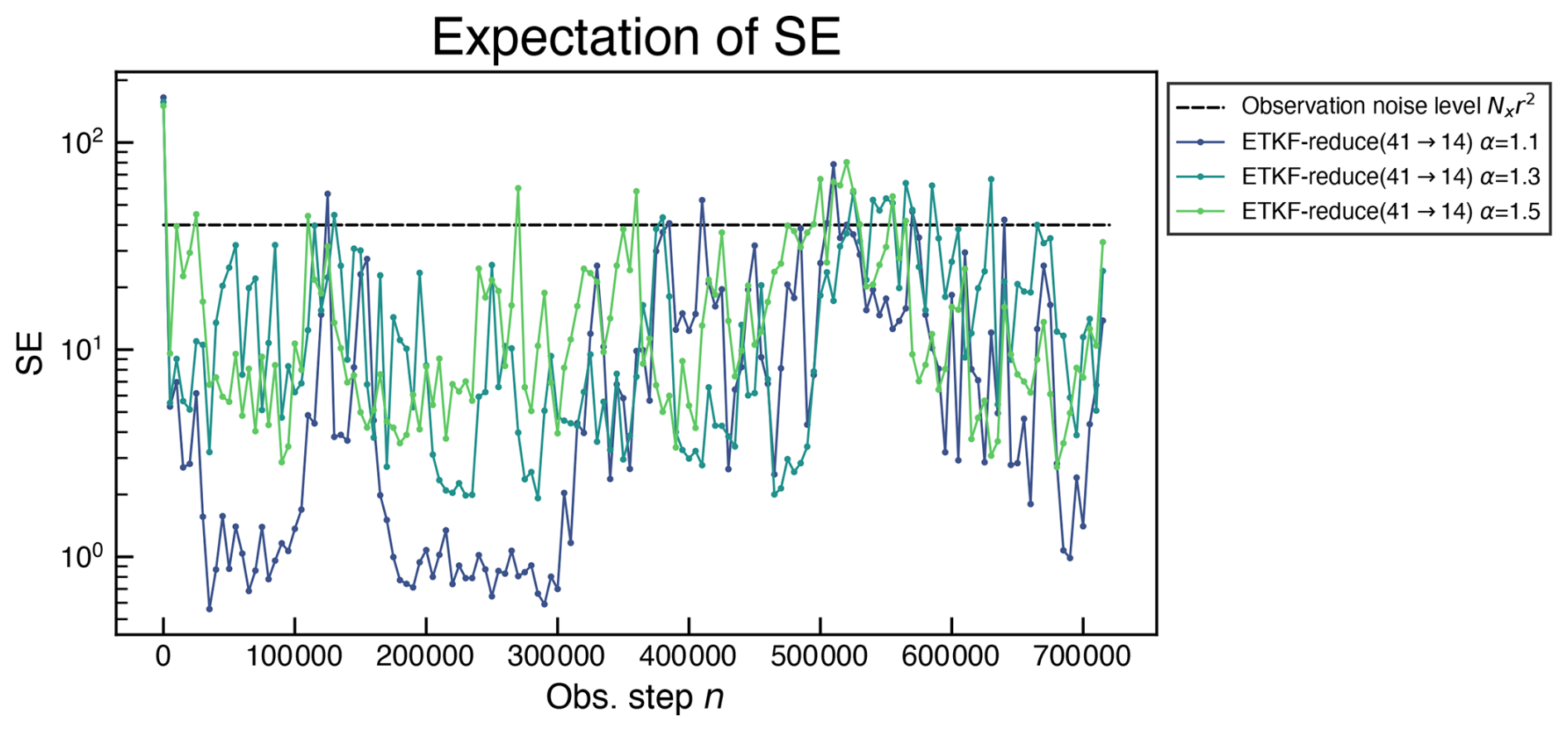
Figure B1 The time series of the SE with r=1.0, m=14, n_obs=1, Δt=0.001, and various α. The dashed line indicates the level N_xr².