The stochastic skeleton model for the Madden–Julian Oscillation with time-dependent observation-based forcing

We analyze solutions to the stochastic skeleton model, a minimal non-linear oscillator model for the Madden–Julian Oscillation (MJO). This model has been recognized for its ability to reproduce several large-scale features of the MJO. In previous studies, the model's forcings were predominantly chosen to be mathematically simple and time-independent. Here, we present solutions to the model with time-dependent observation-based forcing functions. Our results show that the model, with these more realistic forcing functions, successfully replicates key characteristics of MJO events, such as their lifetime, extent, and amplitude, whose statistics agree well with observations. However, we find that the seasonality of MJO events and the spatial variations in the MJO properties are not well reproduced. Having implemented the model in the presence of time-dependent forcings, we can analyze the impact of temporal variability at different timescales. In particular, we study the model's ability to reflect changes in MJO characteristics under the different phases of El Niño–Southern Oscillation (ENSO). We find that it does not capture significant differences in the studied characteristics of MJO events in response to differences in conditions during El Niño, La Niña, and neutral ENSO.

1 Introduction

The Madden–Julian Oscillation (MJO; Madden and Julian, 1972) is the dominant component of intraseasonal variability in the tropics (Woolnough, 2019). It is a planetary-scale wave envelope of smaller-scale convective processes, slowly propagating eastward along the Equator, with a period of 40 to 50 d on average and a mean propagation speed of about 5 m s⁻¹, with fluctuations ranging from 1 to 9 m s⁻¹ (Chen and Wang, 2020). As it propagates, the MJO causes disturbances in rainfall and winds, which impact weather and climate in both the tropics and the extratropics (Zhang, 2013). In particular, the MJO plays a significant role in the occurrence of various weather extremes such as tropical cyclones, tornadoes, extreme rainfall events and extreme surface temperatures (Jones et al., 2004; Pohl and Camberlin, 2006; Juliá et al., 2012; Thompson and Roundy, 2013; Zhang, 2013; Jeong et al., 2005).

With its slow eastward propagation on intraseasonal timescales, the MJO is a key source of subseasonal predictability (Woolnough, 2019; Vitart et al., 2019) and is of utmost importance for enhancing preparedness for such extreme events. Accurately forecasting the MJO has thus become a foremost goal in subseasonal-to-seasonal forecasting. However, even with significant progress in recent years (Lim et al., 2018; Kim et al., 2019; Silini et al., 2021), its representation and predictability in numerical models continue to be a challenging task (Liu et al., 2024). Moreover, a recent study suggests that there is an increased probability of extinction of the MJO after 27 d, which seems to point to an internal mechanism of exhaustion rather than the effect of an external barrier (Corral et al., 2023).

The underlying physical mechanisms that govern the MJO are not yet fully understood (Zhang, 2013). A deeper understanding of these mechanisms is however essential for improving MJO predictions, as they form the foundation for the development of more accurate models. This knowledge gap has motivated the development of data-driven models (Díaz et al., 2023) and simplified low-dimensional physics-based models (Zhang et al., 2020) that aim to capture the key aspects of the MJO's behavior. One such model, known as the skeleton model, provides a framework for investigating some essential dynamics of the MJO.

The skeleton model is a minimal non-linear oscillator model for the MJO, introduced by Majda and Stechmann (2009b). The model is derived from the well-known primitive equations for the dry atmosphere in the tropics, complemented by the modeling of moist convection. It is an idealized model with a minimal number of parameters and a single quadratic non-linearity. Nonetheless, it provides insights into atmospheric dynamics when coupled with moist convection in the tropics and is able to reproduce large-scale features of the MJO, including its slow eastward propagation at about 5 m s⁻¹, its near-zero group velocity, and its horizontal quadrupole vortex structure. Several versions of the model have been developed based on the initial work by Majda and Stechmann (Majda and Stechmann, 2011; Thual et al., 2014; Thual and Majda, 2015, 2016). In particular, adding stochasticity to the initial model, Thual et al. (2014) showed that the skeleton theory also captures the intermittent generation of MJO events and their organization into wave trains with growth and decay.

The model includes two forcing functions, representing latent heating and radiative cooling in the tropics. In the majority of previous studies, these functions were chosen to be mathematically simple, time-independent, and identical (Majda and Stechmann, 2009b, 2011; Thual et al., 2014; Thual and Majda, 2016; Stachnik et al., 2015; Chen and Stechmann, 2016). The aim of the present study is to assess whether the model, forced with more dynamic and observationally grounded functions, can still accurately reproduce key characteristics of MJO events. By using more realistic forcings, our work offers a more robust test of the skeleton model's applicability and relevance in understanding the MJO dynamics as simplified, static forcings might limit the realism of the model's outputs. Our goal is not to predict individual MJO events, which is a challenge for models of much higher complexity (Jiang et al., 2020; Zhou et al., 2024), but to check how well the skeleton model reproduces their statistical properties.

Precisely, we consider the stochastic skeleton model as presented in Thual et al. (2014) with forcing functions computed from observational and reanalysis data following a methodology presented in Ogrosky and Stechmann (2015). Further, while Ogrosky and Stechmann (2015) forced the model with long-term averages of the computed functions, in this work, we keep their time dependence. Thus, we present solutions to the model when the latent heating and radiative cooling functions are observation-based, time-dependent, non-identical functions. To our knowledge, this is the first study of the MJO skeleton model with forcing functions combining these three characteristics.

Further, several studies have suggested that the sea surface temperature (SST) variability at interannual and longer timescales influences the MJO's characteristics. In particular the variability associated with the El Niño–Southern Oscillation (ENSO) modulates the extent of MJO's eastward propagation (Kessler, 2001; Tam and Lau, 2005; Pohl and Matthews, 2007), its lifetime (Pohl and Matthews, 2007), and its speed (Wei and Ren, 2019; Díaz et al., 2023). With our implementation of the skeleton model using time-dependent forcings, we can now explore the ability of the MJO skeleton model to induce differences in selected MJO characteristics under El Niño, La Niña, and neutral ENSO conditions.

This paper is organized as follows. In Sect. 2, we present the model, and in Sect. 3, the computation of the forcing functions from observational and reanalysis data is explained. The identification of MJO events in the model is performed based on an objective index: the skeleton multivariate MJO (SMM) index. The computation of the SMM index is described in Sect. 4. The numerical solutions to the model are then presented in Sect. 5. The identification of MJO events is briefly illustrated in Sect. 6. In Sect. 7, we compare statistics of MJO characteristics between observations and simulations. Finally, in Sect. 8, we present the statistics of selected characteristics of MJO events in observations and in the stochastic skeleton model simulations under El Niño, La Niña, and neutral ENSO conditions.

2 The MJO skeleton model

2.1 Deterministic model

The MJO skeleton model (Majda and Stechmann, 2009b, 2011) combines the linear, longwave-scaled, primitive equations (see White, 2003; Vallis, 2017) with a conservation equation for moisture and a dynamic equation describing the interactions between the lower tropospheric moisture anomaly and the planetary-scale envelope of convective activity

$$\begin{array}{}\text{(1)}& \begin{array}{rl}{u}_{\mathrm{t}}-yv& =-p_x,\\ yu& =-p_y,\\ \mathrm{0}& =-p_z+\mathit{\theta },\\ u_x+v_y+w_z& =\mathrm{0},\\ {\mathit{\theta }}_{\mathrm{t}}+w& =\stackrel{\mathrm{‾}}{H}a-s^{\mathit{\theta }},\\ q_{\mathrm{t}}-\stackrel{\mathrm{̃}}{Q}w& =-\stackrel{\mathrm{‾}}{H}a+s^{\mathrm{q}},\\ a_{\mathrm{t}}& =\mathrm{\Gamma }qa,\end{array}\end{array}$$

where x, y, and z are the zonal, meridional and vertical coordinates, and u, v, and w are the velocity anomalies in these directions, respectively, p and θ are the pressure and potential temperature anomalies, q is the lower tropospheric moisture anomaly, and a is the envelope of convective activity. Note that all variables are anomalies from a radiative–convective equilibrium except for a. The variables s^θ and s^q represent external sinks/sources of temperature and moisture, such as radiative cooling and latent heating, respectively. They act as forcing in the model and will be described in more detail in Sect. 3. The model has only three parameters: $\stackrel{\mathrm{̃}}{Q}$ is the mean background vertical moisture gradient, Γ represents the sensitivity of convective activity tendency to moisture anomalies, and $\stackrel{\mathrm{‾}}{H}$ is a scaling constant for the convective activity. The equations have been non-dimensionalized using some standard equatorial length scales and timescales (Majda and Stechmann, 2009a). The first five equations of the model describe the dry dynamics of the atmosphere (the conservation of horizontal momentum in x and y, the hydrostatic balance, the conservation of mass, and the conservation of potential temperature). The sixth equation describes the conservation of low-level moisture. The last equation is the non-linear interaction between moisture and convection. It entails the idea that the moisture anomalies influence the growth and decay rates of the planetary-scale envelope of convective activity.

To obtain the model in its simplest version (Majda and Stechmann, 2009b, 2011; Thual et al., 2014; Majda et al., 2019, their Sect. 2.3.3), Eq. (1) is truncated in the vertical and meridional directions. In the vertical, the variables are expanded in terms of sines and cosines, keeping only the first baroclinic mode, i.e., $u(x,y,z,t)\approx u_{\mathrm{1}}(x,y,t)\sqrt{\mathrm{2}}\cos \left(z\right)$, $v(x,y,z,t)\approx v_{\mathrm{1}}(x,y,t)\sqrt{\mathrm{2}}\cos \left(z\right)$, $p(x,y,z,t)\approx p_{\mathrm{1}}(x,y,t)\sqrt{\mathrm{2}}\cos \left(z\right)$, $w(x,y,z,t)\approx w_{\mathrm{1}}(x,y,t)\sqrt{\mathrm{2}}\sin \left(z\right)$, and $\mathit{\theta }(x,y,z,t)\approx {\mathit{\theta }}_{\mathrm{1}}(x,y,t)\sqrt{\mathrm{2}}\sin \left(z\right)$ (see Khouider et al., 2013). Here, $z\in [\mathrm{0},\mathit{\pi }]$ in non-dimensional units, and $z\in [\mathrm{0},H_{\text{top}}]$ in dimensional units, where H_top is the height of the tropopause. Further, it is assumed that $q=q_{\mathrm{1}}(x,y,t)\sqrt{\mathrm{2}}\sin \left(z\right)$, $a=a_{\mathrm{1}}(x,y,t)\sqrt{\mathrm{2}}\sin \left(z\right)$, $s^{\mathit{\theta }}=s_{\mathrm{1}}^{\mathit{\theta }}(x,y,t)\sqrt{\mathrm{2}}\sin \left(z\right)$, and $s^{\mathrm{q}}=s_{\mathrm{1}}^{\mathrm{q}}(x,y,t)\sqrt{\mathrm{2}}\sin \left(z\right)$ (see Majda and Tong, 2016). Dropping the subscript 1 for simplicity (i.e., u₁→u, v₁→v, etc.), System (1) becomes

$$\begin{array}{}\text{(2)}& \begin{array}{rl}{u}_{\mathrm{t}}-yv-{\mathit{\theta }}_x& =\mathrm{0},\\ yu-{\mathit{\theta }}_y& =\mathrm{0},\\ {\mathit{\theta }}_{\mathrm{t}}-u_x-v_y& =\stackrel{\mathrm{‾}}{H}a-s^{\mathit{\theta }},\\ q_{\mathrm{t}}+\stackrel{\mathrm{̃}}{Q}(u_x+v_y)& =-\stackrel{\mathrm{‾}}{H}a+s^{\mathrm{q}},\\ a_{\mathrm{t}}& =\mathrm{\Gamma }qa.\end{array}\end{array}$$

In the meridional direction, the variables and forcing functions are expanded using the parabolic cylinder functions {ϕ_m(y)}, e.g. $u(x,y,t)={\sum }_m{u}_m(x,t){\mathit{\varphi }}_m\left(y\right)$, where the first three modes have the form ${\mathit{\varphi }}_{\mathrm{0}}\left(y\right)={\mathit{\pi }}^{-\mathrm{1}/\mathrm{4}}\exp (-y^{\mathrm{2}}/\mathrm{2})$, ${\mathit{\varphi }}_{\mathrm{1}}\left(y\right)={\mathit{\pi }}^{-\mathrm{1}/\mathrm{4}}\sqrt{\mathrm{2}}y\exp (-y^{\mathrm{2}}/\mathrm{2})$, and ${\mathit{\varphi }}_{\mathrm{2}}\left(y\right)={\mathit{\pi }}^{-\mathrm{1}/\mathrm{4}}(\mathrm{1}/\sqrt{\mathrm{2}})(\mathrm{2}{y}^{\mathrm{2}}-\mathrm{1})\exp (-y^{\mathrm{2}}/\mathrm{2})$. This expansion facilitates a change of variable in the dry dynamics (rows 1–4 of Eq. 2) allowing the introduction of new variables representing equatorial waves. In the simplest version of the model, only the amplitudes of the first mode of equatorial Kelvin wave structure (K) and equatorial Rossby wave structure (R) are kept, defined as $K\equiv \frac{u_{\mathrm{0}}-{\mathit{\theta }}_{\mathrm{0}}}{\sqrt{\mathrm{2}}}$ and $R\equiv u_{\mathrm{2}}-{\mathit{\theta }}_{\mathrm{2}}-\frac{u_{\mathrm{0}}+{\mathit{\theta }}_{\mathrm{0}}}{\sqrt{\mathrm{2}}}$. In addition, it is assumed that the envelope of convection/wave activity a takes the form $a(x,y,t)=A(x,t){\mathit{\varphi }}_{\mathrm{0}}\left(y\right)=\left[A_{\mathrm{s}}\right(x)+A^{\ast }(x,t\left)\right]{\mathit{\varphi }}_{\mathrm{0}}\left(y\right)$, with A_s representing the background state and A^∗ fluctuations around this state, and that $q(x,y,t)$, $s^{\mathit{\theta }}(x,y,t)$, and $s^{\mathrm{q}}(x,y,t)$ are truncated at the first mode $q(x,y,t)=Q(x,t){\mathit{\varphi }}_{\mathrm{0}}\left(y\right)$, $s^{\mathit{\theta }}(x,y,t)=S^{\mathit{\theta }}(x,t){\mathit{\varphi }}_{\mathrm{0}}\left(y\right)$, and $s^{\mathrm{q}}(x,y,t)=S^{\mathrm{q}}(x,t){\mathit{\varphi }}_{\mathrm{0}}\left(y\right)$. The final truncated equations then read

$$\begin{array}{}\text{(3)}& \begin{array}{rl}{K}_{\mathrm{t}}+K_x& =-{\displaystyle \frac{\mathrm{1}}{\sqrt{\mathrm{2}}}}(\stackrel{\mathrm{‾}}{H}A-S^{\mathit{\theta }}),\\ R_{\mathrm{t}}-{\displaystyle \frac{\mathrm{1}}{\mathrm{3}}}{R}_x& =-{\displaystyle \frac{\mathrm{2}\sqrt{\mathrm{2}}}{\mathrm{3}}}(\stackrel{\mathrm{‾}}{H}A-S^{\mathit{\theta }}),\\ Q_{\mathrm{t}}+{\displaystyle \frac{\mathrm{1}}{\sqrt{\mathrm{2}}}}\stackrel{\mathrm{̃}}{Q}{K}_x-{\displaystyle \frac{\mathrm{1}}{\mathrm{6}\sqrt{\mathrm{2}}}}\stackrel{\mathrm{̃}}{Q}{R}_x& ={\displaystyle \frac{\stackrel{\mathrm{̃}}{Q}}{\mathrm{6}}}(\stackrel{\mathrm{‾}}{H}A-S^{\mathit{\theta }})-(\stackrel{\mathrm{‾}}{H}A-S^{\mathrm{q}}),\\ A_{\mathrm{t}}& =\mathit{\gamma }\mathrm{\Gamma }Q(A_{\mathrm{s}}+A^{\ast }),\end{array}\end{array}$$

where all the functions depend now only on x and t, and $\mathit{\gamma }=\int ({\mathit{\varphi }}_{\mathrm{0}}{)}^{\mathrm{3}}\mathrm{d}y\approx \mathrm{0.6}$ results from the meridional projection of the non-linear equation.

The variables u, v, and θ can be approximately recovered via

$$\begin{array}{}\text{(4)}& \begin{array}{rl}u(x,y,t)& ={\displaystyle \frac{\mathrm{1}}{\sqrt{\mathrm{2}}}}\left[K(x,t)-{\displaystyle \frac{\mathrm{1}}{\mathrm{2}}}R(x,t)\right]{\mathit{\varphi }}_{\mathrm{0}}\left(y\right)+{\displaystyle \frac{\mathrm{1}}{\mathrm{4}}}R(x,t){\mathit{\varphi }}_{\mathrm{2}}\left(y\right),\\ v(x,y,t)& =\left[{\displaystyle \frac{\mathrm{1}}{\mathrm{3}}}{\partial }_{x}R(x,t)-{\displaystyle \frac{\mathrm{1}}{\mathrm{3}\sqrt{\mathrm{2}}}}\left(\stackrel{\mathrm{‾}}{H}A\right(x,t)-S^{\mathit{\theta }}(x,t\left)\right)\right]{\mathit{\varphi }}_{\mathrm{1}}\left(y\right),\\ \mathit{\theta }(x,y,t)& =-{\displaystyle \frac{\mathrm{1}}{\sqrt{\mathrm{2}}}}\left[K(x,t)+{\displaystyle \frac{\mathrm{1}}{\mathrm{2}}}R(x,t)\right]{\mathit{\varphi }}_{\mathrm{0}}\left(y\right)-{\displaystyle \frac{\mathrm{1}}{\mathrm{4}}}R(x,t){\mathit{\varphi }}_{\mathrm{2}}\left(y\right).\end{array}\end{array}$$

2.2 Stochastic model

In the skeleton model, the MJO is initiated and sustained by the synoptic (sub-planetary)-scale convective activity patterns, which are considered collectively via their planetary-scale envelope a. These synoptic-scale processes include for instance deep convective clouds, which are highly irregular, are intermittent, and have low predictability. To account for such processes, Thual et al. (2014) proposed a modified version of the skeleton model, where the last equation in Eq. (1) is replaced by a stochastic process. The authors showed that this stochastic skeleton model is able to generate intermittent MJO wave trains with growth and decay as observed in reality. Specifically, the variable a in System (1) is replaced at each point by an independent random variable taking discrete values separated by Δa, that is a=ηΔa, with η∈ℕ. The evolution of a is controlled by a birth–death process allowing for intermittent transitions between states η. This process is described by the following master equation for the probability of η, P(η,t):

$$\begin{array}{}\text{(5)}& \begin{array}{rl}{\partial }_{\mathrm{t}}P\left(\mathit{\eta }\right)=& \left[\mathit{\lambda }\right(\mathit{\eta }-\mathrm{1}\left)P\right(\mathit{\eta }-\mathrm{1})-\mathit{\lambda }(\mathit{\eta }\left)P\right(\mathit{\eta }\left)\right]\\ & +\left[\mathit{\mu }\right(\mathit{\eta }+\mathrm{1}\left)P\right(\mathit{\eta }+\mathrm{1})-\mathit{\mu }(\mathit{\eta }\left)P\right(\mathit{\eta }\left)\right],\end{array}\end{array}$$

where λ is the upward rate of transition and μ  is the downward rate. The choice of λ and μ is made such that the dynamics of the non-stochastic skeleton model are recovered on average (see Thual et al., 2014).

3 Observation-based time-dependent forcing functions

As mentioned in the introduction, the majority of previous studies on the MJO skeleton model used idealized, time-independent, and equal forcing functions s^θ (radiative cooling) and s^q (latent heating); i.e., s^θ(x)=s^q(x) (see Majda and Stechmann, 2009b, 2011; Thual et al., 2014; Thual and Majda, 2016; Stachnik et al., 2015; Chen and Stechmann, 2016). Thual et al. (2015) first studied the solutions of the skeleton model with periodic variations in the forcing. The authors used an idealized warm pool state representation of $s^{\mathit{\theta }}(\mathit{x},t)=s^{\mathrm{q}}(\mathit{x},t)$ migrating seasonally in the meridional direction. In Ogrosky and Stechmann (2015) and later in Ogrosky et al. (2017), the authors computed the forcing functions based on long-term means of observational and reanalysis data, leading to more realistic functions where s^θ(x)≠s^q(x).

Here, we consider the stochastic skeleton model, with forcing functions computed from observational and reanalysis data following the methodology presented in Ogrosky and Stechmann (2015). However, unlike Ogrosky and Stechmann, we do not take long-term averages but consider monthly varying data. We are hence concerned with solutions of model (1) when $s^{\mathit{\theta }}=s^{\mathit{\theta }}(\mathit{x},t)$, $s^{\mathrm{q}}=s^{\mathrm{q}}(\mathit{x},t)$, and s^θ≠s^q, that is, when the forcings are realistic (observation-based), time-dependent, and non-identical. We stress that all model parameters were chosen as in Ogrosky and Stechmann (2015). No further parameter tuning has been performed to show more clearly the effect of the new ingredient introduced here: the time-dependent forcing. This section explains the computation of the profiles.

3.1 Data sources

To estimate the forcing terms, we use NCEP/NCAR reanalysis latent heat net flux (Kalnay et al., 1996) for the computation of the latent heating s^q and NCEP Global Precipitation Climatology Project (GPCP) data (Adler et al., 2016; Huffman et al., 2001) for the computation of $\stackrel{\mathrm{‾}}{H}a$ (which then enters into the calculation of both s^q and s^θ as explained below). The chosen data sub-sets cover the period 1979–2021 with a monthly resolution. Both fields have global spatial coverage, with a resolution of 1.875° × 1.875° (degrees of latitude and longitude) for the latent heat flux data set and 2.5° × 2.5° for the precipitation data set.

3.2 Estimation procedure

First, following Ogrosky and Stechmann (2015), the 2D field $\stackrel{\mathrm{‾}}{H}a(x,y)$ is computed using the formula

$$\begin{array}{}\text{(6)}& \stackrel{\mathrm{‾}}{H}a=\left({\displaystyle \frac{g{\mathit{\rho }}_{\mathrm{w}}{L}_{\mathrm{v}}}{p_{\mathrm{0}}{c}_p}}\right)M,\end{array}$$

where M [m] represents the monthly precipitation data, g = 9.8 m s⁻² is the gravitational acceleration constant, ρ_w = 10³ kg m⁻³ is the density of water, L_v = 2.5 × 10⁶ J kg⁻¹ is the latent heat of vaporization, c_p = 1006 J (kg K)⁻¹ is the specific heat of dry air at constant pressure, and p₀ = 1.013 × 10⁵ $\mathrm{kg}{\mathrm{m}}^{-\mathrm{1}}{\mathrm{s}}^{-\mathrm{2}}$ is the mean atmospheric pressure at mean sea level. The above formula describes the rate at which the temperature of a column of air increases from the energy released by precipitation at a given location. To obtain the 1D equatorial profile needed for the truncated model (see Sect. 2, Eq. 3), the 2D field is projected onto the leading meridional mode ϕ₀ as

$$\begin{array}{}\text{(7)}& \stackrel{\mathrm{‾}}{H}A(x,t)=\underset{-\mathrm{\infty }}{\overset{\mathrm{\infty }}{\int }}\stackrel{\mathrm{‾}}{H}a(x,y,t){\mathit{\varphi }}_{\mathrm{0}}\left(y\right)\mathrm{d}y.\end{array}$$

Second, still following Ogrosky and Stechmann (2015), we compute the 1D equatorial forcing profile S^q(x,t). The latent heat flux (LHF) is projected onto ϕ₀,

$$\begin{array}{}\text{(8)}& {\text{LHF}}_{\mathrm{0}}(x,t)=\underset{-\mathrm{\infty }}{\overset{\mathrm{\infty }}{\int }}\text{LHF}(x,y,t){\mathit{\varphi }}_{\mathrm{0}}\left(y\right)\mathrm{d}y,\end{array}$$

and S^q is computed according to Ogrosky and Stechmann (2015) as

$$\begin{array}{}\text{(9)}& S^{\mathrm{q}}=H_{\text{LHF}}\cdot {\text{LHF}}_{\mathrm{0}},\end{array}$$

where

$$H_{\text{LHF}}\approx {\displaystyle \frac{\langle \stackrel{\mathrm{‾}}{H}A{\rangle }_{t,x}}{\langle {\text{LHF}}_{\mathrm{0}}{\rangle }_{t,x}}}\approx \mathrm{0.0067}\mathrm{K}{\mathrm{d}}^{-\mathrm{1}}({\mathrm{Wm}}^{-\mathrm{2}}{)}^{-\mathrm{1}},$$

with $\langle \cdot {\rangle }_{t,x}$ representing the time and zonal mean, implying that $\langle \stackrel{\mathrm{‾}}{H}A\rangle$ balances 〈S^q〉.

In fact, according to Ogrosky and Stechmann (2015) (Eq. 7 in that paper), for a steady-state solution to exist in the skeleton model, which has no damping, we must have

$$\begin{array}{}\text{(10)}& \langle \stackrel{\mathrm{‾}}{H}{A}_{\mathrm{s}}{\rangle }_x={〈S_{\mathrm{s}}^{\mathrm{q}}〉}_x={〈S_{\mathrm{s}}^{\mathit{\theta }}〉}_x,\end{array}$$

where 〈⋅〉_x represents the zonal mean and the subscript s indicates the background state of the quantities, defined as their long-time average. From Eq. (9), we see that this is satisfied for $\stackrel{\mathrm{‾}}{H}A$ and S^q.

In addition, as explained in Ogrosky and Stechmann (2015) (Eq. 8 in that paper), the model background convective activity must satisfy

$$\begin{array}{}\text{(11)}& \stackrel{\mathrm{‾}}{H}{A}_{\mathrm{s}}={\displaystyle \frac{S_{\mathrm{s}}^{\mathrm{q}}-\stackrel{\mathrm{̃}}{Q}{S}_{\mathrm{s}}^{\mathit{\theta }}}{\mathrm{1}-\stackrel{\mathrm{̃}}{Q}}}.\end{array}$$

To make sure that this is the case, we compute S^θ(x,t) as

$$\begin{array}{}\text{(12)}& S^{\mathit{\theta }}={\displaystyle \frac{\mathrm{1}}{\stackrel{\mathrm{̃}}{Q}}}{S}^{\mathrm{q}}-{\displaystyle \frac{(\mathrm{1}-\stackrel{\mathrm{̃}}{Q})}{\stackrel{\mathrm{̃}}{Q}}}\stackrel{\mathrm{‾}}{H}A.\end{array}$$

Note that, computed in this way, S^θ also automatically satisfies condition (10).

The computed functions A_s, S^q, and S^θ can be decomposed into spatial Fourier modes. In order to focus on planetary-scale variations, only the first eight Fourier modes are kept.

The aim of this work is to study the solutions to the MJO skeleton model when the forcing functions are time-dependent observation-based functions. Therefore, while Ogrosky and Stechmann (2015) used long-term averages of the computed S^q and S^θ, here we skip this step and keep the time dependence of the profiles. As mentioned above, the datasets have a monthly resolution. Nonetheless, it was observed that using monthly varying profiles causes a drop in the frequency of model-generated MJO events. Hence, as the model seems to require a degree of persistence in duration and amplitude of the forcing to adequately generate MJO events, we smooth the forcing functions in time using a 3-month running mean. Further clarifying the specific factors that cause the studied conceptual model's failure to exhibit a reasonable frequency of MJO events when employing the time-dependent forcing without smoothing, as well as the impact of the smoothing timescale on the statistical properties of the generated events, requires further numerical as well as analytical study of the model. We suggest that those points should be clarified in targeted follow-up studies.

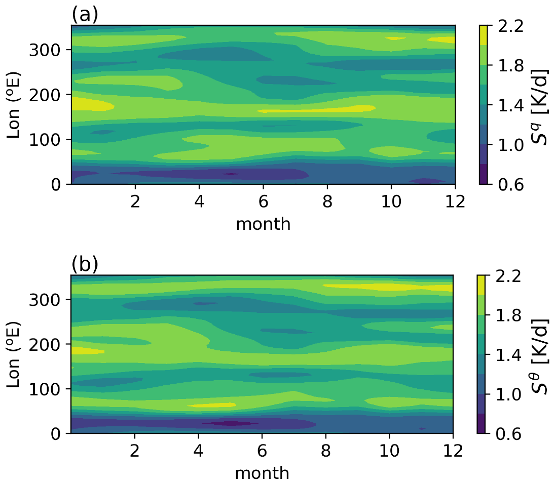
The 3-month smoothed profiles are finally interpolated to the time step of the model. We therefore obtain smooth time-dependent observation-based forcing functions S^q and S^θ. As an example, their evolution over the year 1979 is illustrated in Fig. 1.

Figure 1 Evolution of (a) the latent heating profile S^q estimated from latent heat flux and (b) the radiative cooling profile S^θ computed according to Eq. (12). The abscissa indicates months of the year 1979.

4 Identification of MJO events: the skeleton multivariate MJO index

In observations, the most commonly used index to monitor the MJO is the real-time multivariate MJO (RMM) index developed by Wheeler and Hendon (2004). It is based on an empirical orthogonal function (EOF) analysis of the daily observed outgoing longwave radiation (OLR) as well as lower tropospheric (850 hPa) and upper tropospheric (200 hPa) zonal winds, averaged meridionally in the equatorial region between 15° S and 15° N. The index is typically represented in a two-dimensional phase space defined by the two dominant principal components (RMM1 and RMM2). This space is divided into eight sectors, each corresponding to a distinct phase of the MJO cycle as its convective center travels from the Indian Ocean across the Pacific and towards the Western Hemisphere.

In order to objectively identify MJO structures in the model output, we compute an index similar to the RMM index following the methodology presented in Stachnik et al. (2015). The main difference is that while RMM uses three variables (upper and lower tropospheric winds and OLR), the model index is based on a bivariate analysis with the (model) zonal wind u as a direct substitute for the lower tropospheric wind and the negative convective heating $-\stackrel{\mathrm{‾}}{H}a$ as a proxy for OLR. Since clouds affect the radiation emitted at the top of the atmosphere, OLR is often chosen as an indicator of cloudiness. Wheeler and Hendon (2004) used OLR as a proxy for convective activity, justifying the choice of $-\stackrel{\mathrm{‾}}{H}a$ herein.¹ The steps for the computation of this skeleton multivariate MJO (SMM) index are briefly described below, and full details can be found in Stachnik et al. (2015).

We first isolate the intraseasonal signal in the data. To do so, daily anomalies of u and $-\stackrel{\mathrm{‾}}{H}a$ are filtered using a 20–100 d Lanczos filter. Second, each field is normalized by its global standard deviation so that it has an equal contribution in the computation of empirical orthogonal functions. Lastly, as in Wheeler and Hendon (2004), the model principal components SMM1 and SMM2 are computed by projecting the filtered data onto the two leading EOF modes and standardizing the output such that a value of unity represents an anomaly of 1 standard deviation from the mean.

Strong MJO activity is characterized by an index amplitude greater than or equal to 1. Precisely, following Stachnik et al. (2015), MJO events or episodes are defined from the (SMM1,SMM2) time series as periods during which the following conditions are met:

• The amplitude of SMM is greater than 1: $\sqrt{\text{SMM}{\mathrm{1}}^{\mathrm{2}}+\text{SMM}{\mathrm{2}}^{\mathrm{2}}}\ge \mathrm{1}$.

• The propagation of the event is almost continually counterclockwise in the (SMM1, SMM2) space, corresponding to an almost continually eastward propagation (a westward propagation is limited to at most a single phase of the MJO cycle).

• The event propagates through at least four phases of the MJO cycle.

5 Numerical solution

In this section, we present the main features of the numerical solution to the stochastic MJO skeleton model (3) with (dimensionless) parameters $\stackrel{\mathrm{̃}}{Q}=\mathrm{0.9}$, Γ=1.0, and $\stackrel{\mathrm{‾}}{H}=\mathrm{0.22}$, as in Ogrosky and Stechmann (2015), and observation-based time-dependent sources of cooling and moistening S^θ and S^q. The spatio-temporal resolution of the model is chosen as in Thual et al. (2014), with the spatial step Δx≈ 625 km (that is $\mathrm{40}\mathrm{000}/\mathrm{64}$, where 40 000 km approximates the circumference of the Earth at the Equator) and the temporal step Δt≈ 1.7 h. Stochasticity is implemented by applying an independent replica of the stochastic process described in Sect. 2.2 to each spatial point x. Our Julia implementation of the model is available from Ehstand (2025). To make sure that the solutions are presented for a statistically equilibrated regime, we run simulations for 215 years with forcing corresponding to the 43-year period 1979–2021 repeated 5 times ($\mathrm{5}\times \mathrm{43}=\mathrm{215}$). We then keep only the last 43 years which we consider representative of the 1979–2021 period.

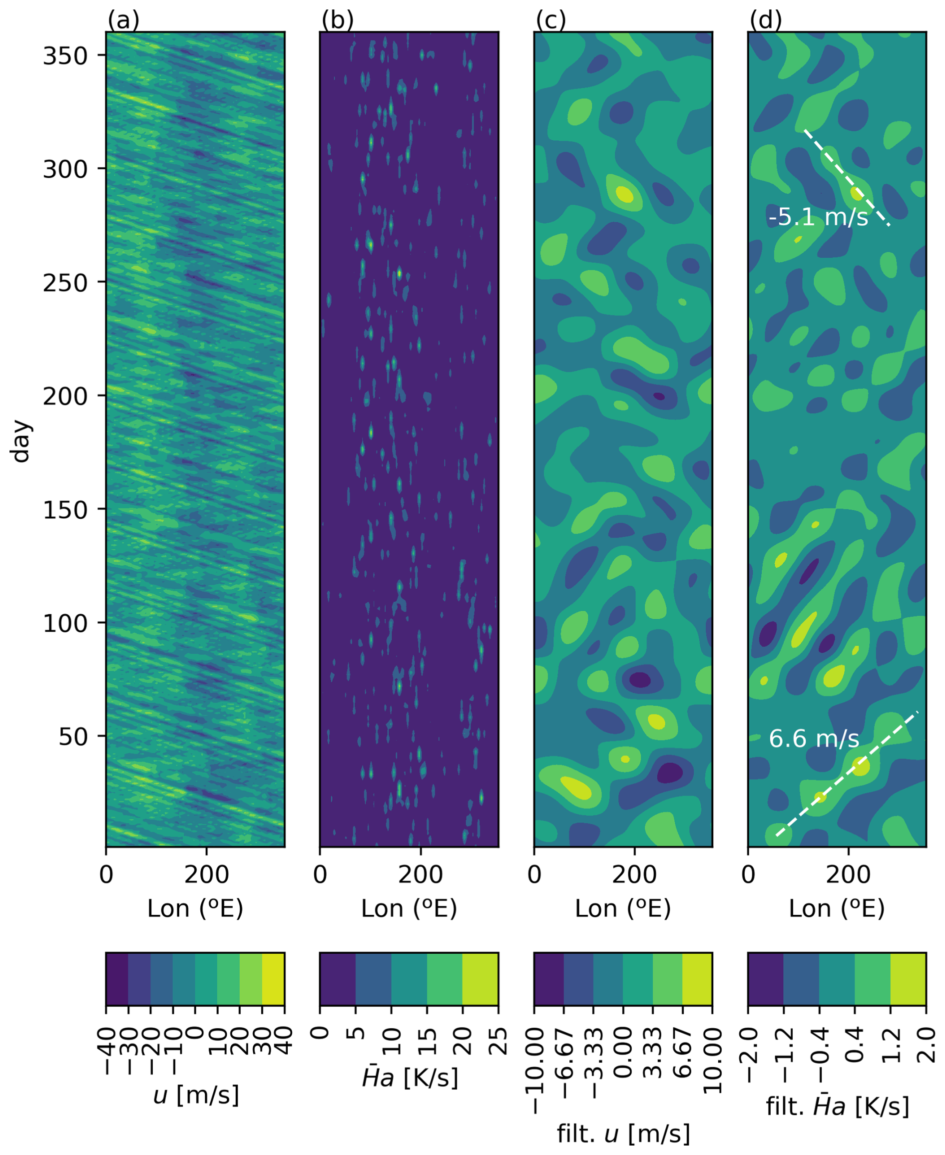
Figure 2 Hovmöller diagrams of the skeleton model lower tropospheric wind $u(x,y=\mathrm{0},t)$ and envelope of convective activity $\stackrel{\mathrm{‾}}{H}a(x,y=\mathrm{0},t)$ at the equator. (a, b) Raw data, (c, d) daily anomalies from the long-term mean, filtered in time and space as described in the text. One westward-moving signal (likely of a moist Rossby wave) and one eastward-moving signal (likely MJO activity) are marked in white in panel (d).

5.1 Hovmöller diagrams of the model variables

The evolution of the skeleton model equatorial profiles for the lower tropospheric wind u(x,t) and envelope of convective activity $\stackrel{\mathrm{‾}}{H}a(x,t)$, computed from Eq. (4) with y=0, are shown in Fig. 2. The time axis represents 1 year of simulation with forcing profiles representative of the year 2005. Figure 2a and b represent the raw output data. Figure 2c and d show the data after filtering in time and space as to isolate planetary-scale intraseasonal variations. Precisely, the daily anomalies from the long-term mean have been filtered in time using a 20–100 d Lanczos filter and smoothed in space by retaining only modes with Fourier wave number k≤4. While the non-filtered plots (Fig. 2a and b) highlight the small-scale propagating waves, the filtering (Fig. 2c and d) allows to capture larger-scale features.

Westward-propagating modes are well visible in Fig. 2a, as well as in Fig. 2c and d, e.g., around days 260 to 300. With periods ranging from around 25 to 90 d, these modes could be related to equatorial Rossby waves (see also Sect. 5.2). On the other hand, large-scale eastward propagating waves are visible in Fig. 2c and d, especially towards the beginning of the period, from day 0 to 150. These intraseasonal large-scale waves are likely associated with the MJO, as we will see in Sect. 5.2. Two waves, one propagating eastward and one propagating westward, have been marked in Fig. 2d with their respective phase speeds. Finally, we observe that in the convective activity plots (Fig. 2b and d), a higher activity can be seen in the region from 60 to 200° E, which corresponds to a region between the Indian Ocean and the western Pacific, which is the region where the MJO signal is usually the strongest.

5.2 Power spectrum of the envelope of convective activity

Figure 3 shows the zonal wavenumber–frequency power spectrum of the simulated (unfiltered) envelope of convective activity $\stackrel{\mathrm{‾}}{H}a$. The zonal wavenumbers are expressed as multiples of $\mathrm{2}\mathit{\pi }/\mathrm{40}\mathrm{000}\mathrm{km}$ and frequencies are in cycles per day (cpd). The dashed lines indicate the 90 and 30 d periods. The MJO appears as a horizontally elongated high power structure in the zonal wavenumber spectrum with $\mathrm{1}\le k\le \mathrm{5}$, that is as a planetary-scale wave, with intraseasonal frequencies $\mathrm{1}/\mathrm{90}\le \mathit{\omega }\le \mathrm{1}/\mathrm{30}\mathrm{cpd}$ and eastward propagation ($\mathit{\omega }/k>\mathrm{0}$). This structure has a dispersion relation $d\mathit{\omega }/dk\approx \mathrm{0}$ which is a typical characteristic of the MJO and is known to be reproduced well by the skeleton model (Majda and Stechmann, 2009b, 2011; Thual et al., 2014). The mean phase speed of the waves associated with this structure (calculated as the mean of $\mathit{\omega }/k$ for the points with $\mathit{\omega }\in [\mathrm{1}/\mathrm{90},\mathrm{1}/\mathrm{30}]$ cpd, $k\in [\mathrm{1},\mathrm{5}]$, and log power greater than −4.0) is ≈ 5 ms⁻¹. This MJO signal is visible in Fig. 2d between days 1 and 150. In addition to the MJO signal there is also a high power structure at intraseasonal timescales with westward propagation. Previous studies have shown that these modes share some, although incomplete, features with convectively coupled equatorial Rossby waves, and they have been referred to as moist Rossby modes (Majda and Stechmann, 2011; Thual et al., 2014). An example of such a westward wave is visible in the filtered convective activity in Fig. 2d between days 260 and 300. At higher frequencies, ω>0.06 cpd corresponding to periods shorter than 16 d, the high power peaks might be associated with dry Kelvin and dry Rossby modes (Majda and Stechmann, 2011; Thual et al., 2014). Overall the spectrum of $\stackrel{\mathrm{‾}}{H}a$ agrees well with previous studies of the skeleton model (Thual et al., 2014; Ogrosky and Stechmann, 2015). While several equatorial modes, and especially the MJO, are well represented, many modes are not reproduced by the model due to its minimal design, for instance convectively coupled Kelvin waves (Kiladis et al., 2009).

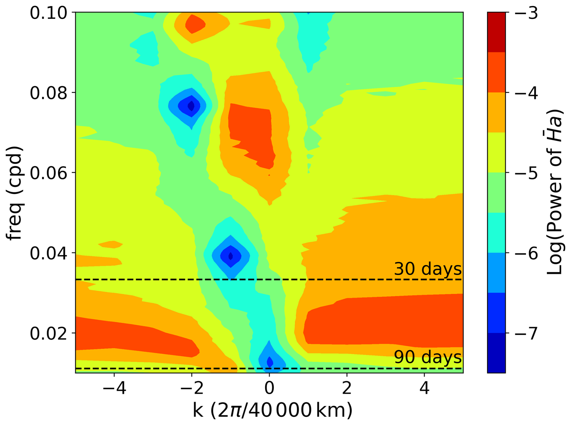
Figure 3 Zonal wavenumber–frequency power spectrum of the simulated envelope of convective activity $\stackrel{\mathrm{‾}}{H}a$ (in base 10 – logarithm). The dashed lines mark the 90- and 30- d periods.

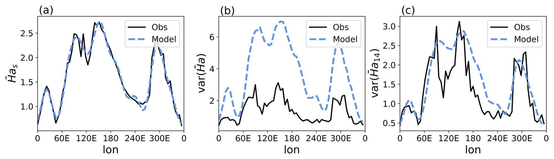
Figure 4 (a) Long-term averages of observed and modeled $\stackrel{\mathrm{‾}}{H}a$ (envelope of convective activity). (b) Variance of modeled and observed $\stackrel{\mathrm{‾}}{H}a$ when all spatial modes from the model output are kept. (c) Variance of modeled and observed $\stackrel{\mathrm{‾}}{H}a$ when only the first 14 spatial modes from the model output are kept. Note the different scales in panels (b) and (c).

5.3 Climatology and variance of the envelope of convective activity

The long-term means of $\stackrel{\mathrm{‾}}{H}a$ estimated from daily observations and simulated in the skeleton model are shown in Fig. 4a. Qualitatively, they agree well. However, the variance of $\stackrel{\mathrm{‾}}{H}a$ is overestimated in the model as can be seen in Fig. 4b. Nonetheless, if we consider only the first 14 spatial modes, the variance is well reproduced by the model (Fig. 4c). This might be explained by the fact that the equations of the skeleton model are longwave-scaled, as the model is only concerned with planetary scales, and hence it might not be well suited to represent modes with higher wavenumbers (which are nevertheless continuously excited by the stochastic dynamics of the convective activity). The appropriate number of long-wavelength modes to be retained in the model's output in order to achieve agreement with observations has been determined empirically, and its justification would need a more detailed modeling approach in which smaller scales would be consistently included.

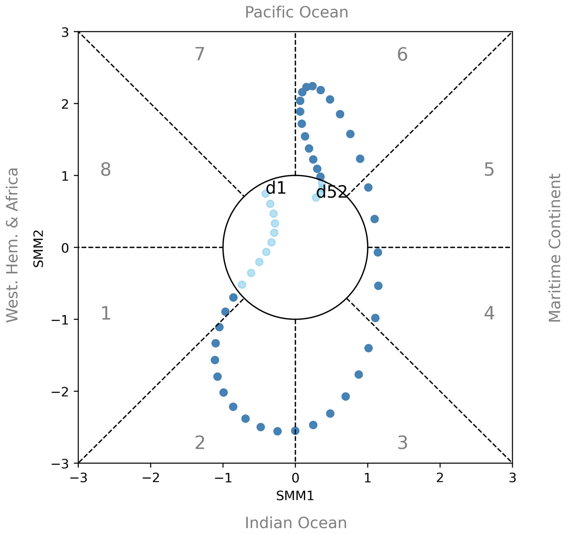
Figure 5 Phase-space diagram of the model SMM values for a 52- d period from a simulation forced with observation-based functions. The dots correspond to daily values of (SMM1, SMM2). The first day of the series is labeled “d1,” and the last is labeled “d52”. The circle in the center of the plot has unit radius, indicating the threshold at which the amplitude of SMM exceeds 1. Points in dark blue indicate an MJO event as defined by the criteria in Sect. 4.

6 Identification of MJO events with the SMM index

The results presented above suggest the presence of intermittent MJO wave structures propagating eastward. In order to objectively identify these structures, we use the skeleton multivariate MJO (SMM) index presented in Sect. 4.

An example of model SMM values over a 52- d period is shown in the (SMM1, SMM2) phase space in Fig. 5. The first and last points of the series are annotated. The dark blue points satisfy the MJO event's criteria given in Sect. 4. Overall, the MJO propagation is relatively smooth. As explained in Stachnik et al. (2015), this is partly due to the filtering of high frequencies in the model SMM index computation. This filtering eliminates some of the day-to-day variability and noise that are not removed in the computation of the observation-based RMM index from Wheeler and Hendon (2004).

7 MJO characteristics in the skeleton model and in observations

In the following, we study different characteristics of the MJO events in simulations and observations. The aim is to assess the ability of the MJO skeleton model to statistically reproduce the characteristics of observed MJO events. Here we list the chosen characteristics.

• The seasonal variation in the occurrence of MJO events is obtained by recording the number of MJO events occurring (that is, starting, continuing, or ending) during each month of the year, where events are defined according to the criteria listed in Sect. 4.

• The duration of an event is defined as the number of days from the first to the last day of the event.

• We measure the total angle covered by an event tracked in the (SMM1, SMM2) phase space, that is the angle covered between the first and the last day of the event. This can roughly be assimilated to the “distance” covered by that event as it propagates along the equator.

• The maximum value of SMM amplitude, where the amplitude is defined as $\sqrt{\text{SMM}{\mathrm{1}}^{\mathrm{2}}+\text{SMM}{\mathrm{2}}^{\mathrm{2}}}$, is recorded for each event.

• Finally, the starting and ending phases of each event (1–8) are recorded.

The model MJO events are identified using the SMM index and the criteria described in Sect. 4. We perform 15 independent simulation runs (in a statistically equilibrated regime) with forcing profiles representative of the period 1979–2021, leading to a total of 980 modeled events. The observed events are computed according to the same criteria using the RMM index values, which are freely available on the website of the Australian Bureau of Meteorology (http://www.bom.gov.au/climate/mjo/). We find 153 observed events over the period 1979–2021. For these observed events, the computation of the characteristics listed above is made from the (RMM1, RMM2) values.

7.1 MJO seasonal variations

We first look at the seasonal variation of MJO occurrences in the model and in observations in Fig. 6. Observations show that MJO events are more frequent during boreal winter and spring, from December through May. In the simulations, however, no variation is detected. Recall that the forcing profiles have been averaged with a 3-month window. As a result, the seasonal variations in heating and moistening are smoother and of reduced amplitude, so that the differences between different seasons might be lost.

Figure 6 Occurrence of MJO events as a function of the month of the year.

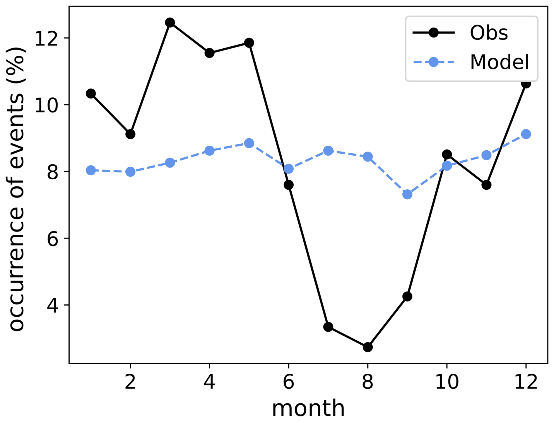
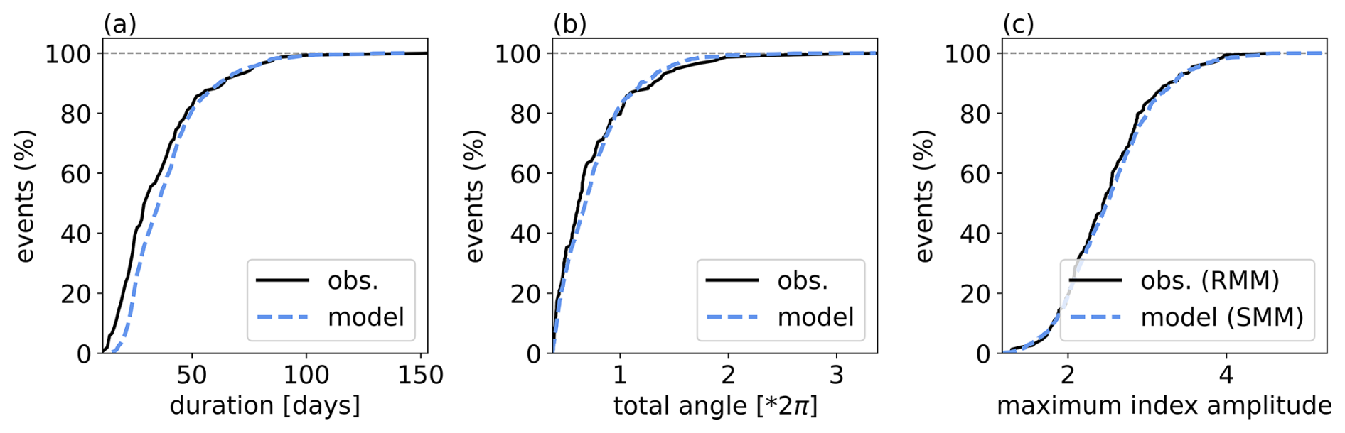
Figure 7 Cumulative probability distribution of (a) the MJO events' durations, (b) total angle covered in (RMM1, RMM2)/(SMM1, SMM2) phase space, and (c) maximum RMM/SMM value for observed and simulated MJO events (981 simulated events and 153 observed events).

7.2 MJO lifetime, extent in SMM/RMM phase space, and maximum SMM/RMM amplitude

We now compare the duration of MJO events, the total angle covered in SMM/RMM phase space, and the maximum SMM/RMM amplitude in the model outputs and in observations. The cumulative probability distributions of these three characteristics are shown in Fig. 7. As above, the statistics are based on 153 observed events over the period 1979–2021 and 980 modeled events from 15 independent simulations, run with forcing profiles representative of the same period. The duration of events in Fig. 7a, the total angle (distances) covered by simulated events in Fig. 7b, and the maximum amplitude of SMM/RMM in Fig. 7c compare well with observations. The average MJO event lifetime is 39.6 ± 0.8 d for the simulation and 36.1 d for observations. This small difference is likely explained by the absence of certain sources of MJO termination in the minimalistic skeleton model leading to slightly longer events (although the longest event overall, of 153 d, occurs in observational data). For comparison, the average event lifetime when time-independent forcings are used (i.e., when the model is forced with the long-term averages of the computed S^q and S^θ) is 40.9 ± 0.7 d, indicating a (small) improvement by using the more realistic time-dependent forcings. The mean angle is $(\mathrm{0.75}\pm \mathrm{0.01})\cdot \mathrm{2}\mathit{\pi }$ for simulations and 0.75⋅2π for observations. This is an improvement with respect to the time-independent-forcing result of $(\mathrm{0.78}\pm \mathrm{0.01})\cdot \mathrm{2}\mathit{\pi }$. The mean of the maxima of SMM amplitude is 2.53±0.02 for the simulations (both with time-dependent and time-independent forcings), and the mean of the maxima of RMM amplitude is 2.50 for observations.

For each of the characteristics, a two-sample Kolmogorov–Smirnov test was conducted to compare the empirical cumulative distribution functions obtained from observations and from the time-dependent-forcing model. The test's null hypothesis is that observed and modeled samples come from the same underlying distribution. For the duration, the test yields a p value of 0.0006, leading to the rejection of the null hypothesis and suggesting that the distributions might differ despite apparent similarities. For the total angle covered in the SMM/RMM phase space, p=0.0428, which also leads to the rejection of the null hypothesis at the 5 % significance level, although differences are less pronounced. For the maxima of SMM/RMM amplitude values, the p-value is 0.8116, indicating that the model and observations produce statistically indistinguishable distributions.

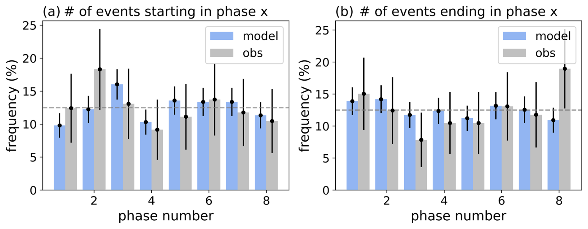
Figure 8 Histograms of the recorded starting (a) and ending phases (b) of MJO events in the model and in observations. The dashed line indicates the equal likelihood of the ending location of an event being recorded in any of the 8 bins. The error bars indicate the 98 % uncertainty estimate, calculated from a binomial proportion confidence interval.

7.3 MJO starting and ending phases

Figure 8 shows the distribution of initial and final phases of MJO events. The error bar for a given bin is calculated using a binomial proportion confidence interval dependent on the pass and fail rate of recorded locations being assigned to that particular bin. The dashed line indicates the equal likelihood of the ending location of an event being recorded in any of the 8 bins. Almost all error bars overlap this line, in both the simulations and the observations, indicating that these graphs do not allow for statistically significant conclusions to be drawn. We note, nonetheless, that the distribution of starting phases might have some similarities. Two local maxima are observed around phases $\mathrm{2}/\mathrm{3}$ and $\mathrm{6}/\mathrm{7}$ for the starting location (although a high peak is also shown in phase 5 for the model, which is not present in observations). For the ending phases, in observations, most of the events end in phase 8, whereas in the model, the peak in phase 8 is relatively small.

To conclude Sect. 7, the time-dependent stochastic skeleton model captures reasonably well statistical features of the MJO events, such as the distributions of durations, total angles covered in SMM/RMM phase space, and the maxima of SMM/RMM values, despite some disparities. However, it does not reproduce well seasonal variations in the MJO occurrences. Nor does it seem to be able to reproduce spatial differences in the MJO properties, such as its starting and ending phase, although more investigation would be needed to establish the presence of statistically significant differences. In the next section, we assess the ability of the model to produce differences in the distributions of durations, total angles, and SMM maxima under El Niño, La Niña, and neutral ENSO conditions. Note that despite the model not being able to reproduce seasonal variations, MJO events might still be influenced by ENSO variations since they occur on much longer timescales (typically of 2 to 7 years, although ENSO itself also varies seasonally in intensity).

8 Modulation of the MJO by ENSO

Equipped with our implementation of the stochastic skeleton model suitable to incorporate time-dependent observation-based forcings, we now study changes in the statistics of selected MJO characteristics under the different phases of ENSO (El Niño, La Niña, and neutral phase) in observations and in the model.

To identify the ENSO phase during the period 1979–2021, we use the NOAA Oceanic Niño Index (ONI), based on SST anomalies in the Niño 3.4 region from 5° S–5° N and 170–120° W. The index is computed by averaging the monthly values of Niño 3.4 SST anomalies with a running 3-month window. An El Niño event is declared when the index is greater than or equal to 0.5 °C for at least five consecutive values, i.e., five consecutive overlapping 3-month seasons. A La Niña event is declared when the index is less than or equal to −0.5 °C for at least five consecutive values. The Niño 3.4 values are available on the website of NOAA (https://origin.cpc.ncep.noaa.gov/products/analysis_monitoring/ensostuff/ONI_change.shtml).

Identifying MJO events that occurred during each of the ENSO phases is straightforward for observational data, based on the event's date. Precisely, the whole length of the MJO event is considered. An event is said to have occurred during El Niño/La Niña/neutral ENSO if more than half of the event has occurred during that specific phase. For the model, as explained in Sect. 5, simulations are run with forcing corresponding to the period 1979–2021, resulting in time-stamped outputs that are considered representative of this period. We can then also identify simulated MJO events occurring during El Niño, La Niña, and neutral ENSO phases based on their dates. In addition, whereas in observations the number of MJO events is constrained to a single 43-year record, limiting the significance of statistical studies, we realize 15 independent runs of the model, obtaining much larger samples and more robust statistical results. The total number of MJO events in observations and in the model runs during each phase of ENSO is reported in Table 1.

Table 1 Number of MJO events in observations and in the model during each phase of ENSO.

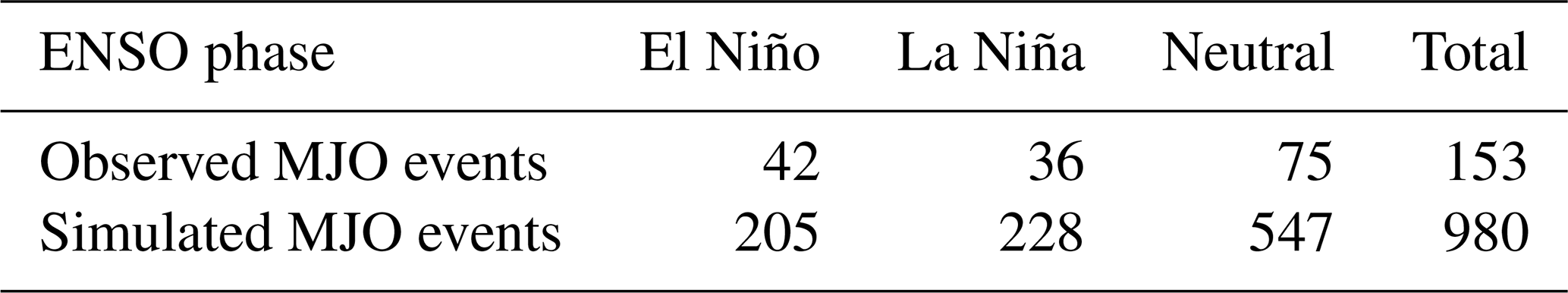
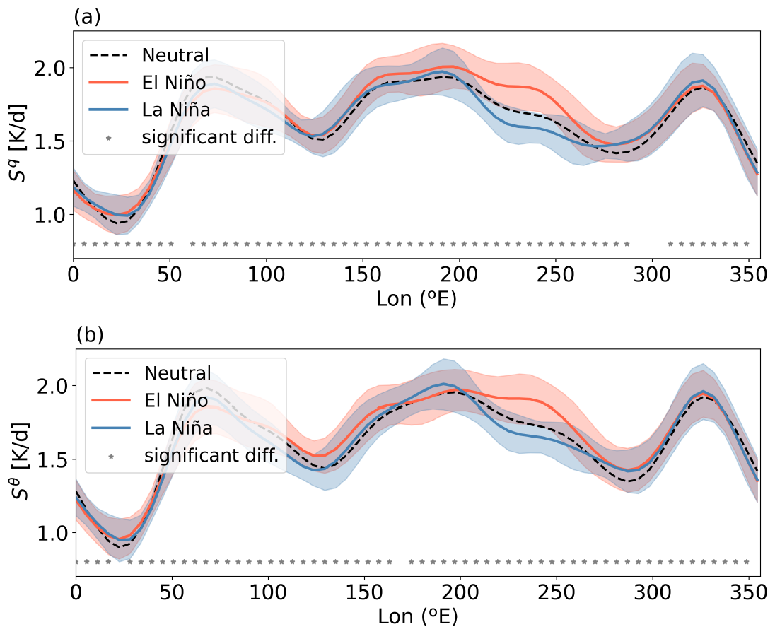
Figure 9 Mean profiles of (a) latent heating (S^q) and (b) radiative cooling (S^θ), during El Niño, La Niña, and neutral ENSO conditions from 1979 to 2021. The shaded areas correspond to 1 standard deviation around the means. Stars indicate locations where forcing profiles differ significantly (at the 5 % significance level) during El Niño and La Niña.

To assess the ability of the stochastic skeleton model to reproduce the observed modulation of MJO activity and characteristics under different ENSO phases, it is essential that the forcing functions S^q and S^θ adequately capture ENSO variability. Figure 9 shows that this is indeed the case by presenting the mean S^q and S^θ profiles during El Niño, La Niña, and neutral ENSO conditions. The largest differences are effectively observed in the eastern equatorial Pacific. Furthermore, we used the Kolmogorov-Smirnov test to assess, at each spatial point, whether the distributions of S^q (S^θ) values differ significantly during El Niño and La Niña. We found significant differences at nearly all points at the 5 % significance level (indicated by stars in the figure).

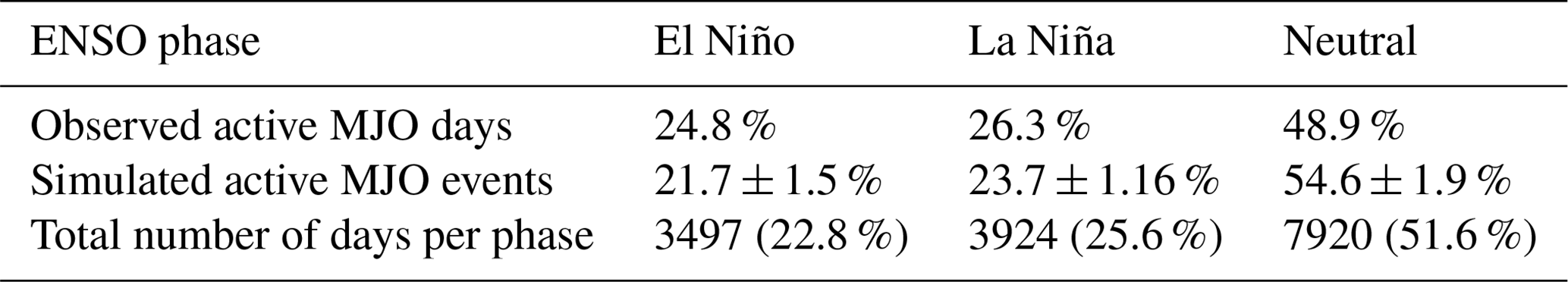
Table 2 Comparison of observed and simulated percentages of active MJO days across ENSO phases – percentages from the total of active MJO days, where “active MJO days” are the days during MJO events as defined in Sect. 4. The last line represents the total number of days (active and inactive MJO) in each phase of ENSO over the period 1979–2021.

8.1 MJO activity across El Niño, La Niña, and neutral ENSO

We first report the occurrence of MJO events across ENSO phases for observations and simulations. Table 2 shows the percentage of MJO active days during El Niño, La Niña, and neutral ENSO for the period 1979–2021 (in observations and simulations). Note that, for the simulations, the values correspond to a mean over the 15 independent runs, and the standard error of the mean is indicated. In addition, the total number of days (irrespective of MJO activity) belonging to each of the three phases is indicated in the last row. We observe that the proportion of MJO days approximately follows the proportion of the total number of days belonging to each phase of ENSO, for both observations and simulations, with the majority of events occurring during the neutral phase of ENSO and the minimum during El Niño. When comparing percentages in the first row with those in the last row, we see that, in observations, El Niño and La Niña conditions seem to slightly favor the occurrence of MJO events (with respect to what would be expected from the proportion of these ENSO phases). On the other hand, when comparing the second row to the last, we see that, in the simulations, the opposite is observed: the neutral ENSO conditions seem to slightly favor the occurrence of MJO events. This small discrepancy could be attributed to the design of the model, i.e., the omission of certain mechanisms and interactions with other climate phenomena, though the differences are minor and may simply reflect limited sample sizes.

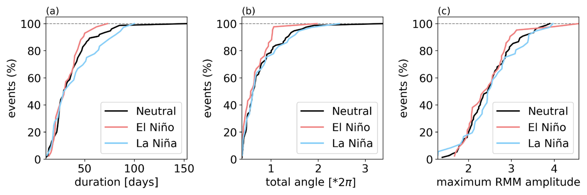
Figure 10 Cumulative probability distribution of (a) the MJO events' durations, (b) total angle covered in (RMM1, RMM2) phase space, and (c) maximum RMM value for observed events occurring during El Niño, La Niña, and neutral periods between 1979 and 2021. The number of events in each sample is reported in Table 1.

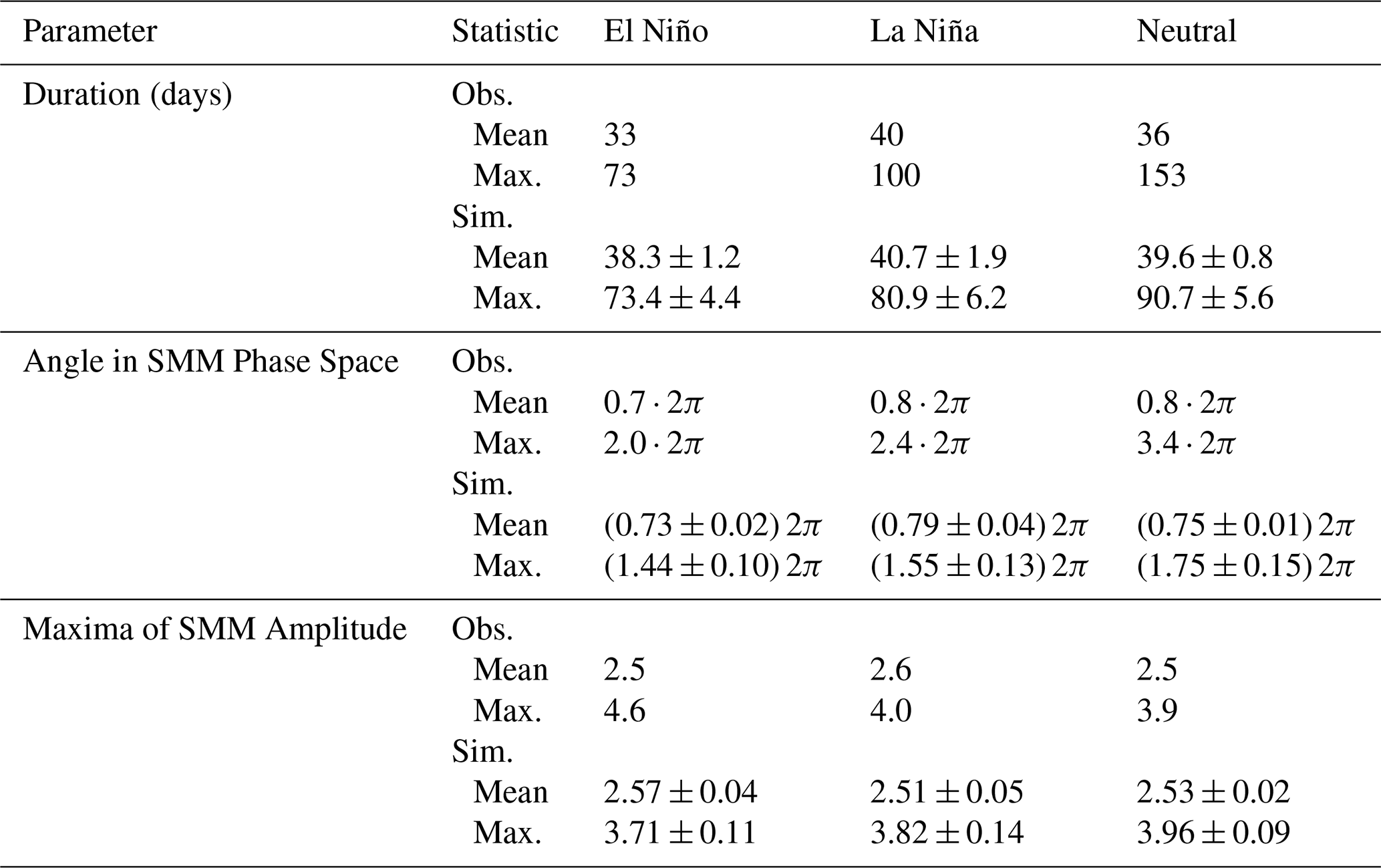
Table 3 Comparison of the mean and maximum values of selected MJO characteristics between observations and simulations. For observations, the values are calculated as a mean over 15 independent simulation runs with the corresponding standard error.

8.2 ENSO modulation of MJO characteristics

8.2.1 Observations

Figure 10 shows the cumulative probability distribution of the MJO events' durations, total angle covered in (RMM1, RMM2) phase space, and maximum RMM value for observed events occurring during El Niño, La Niña, and neutral periods. The distributions show several differences. During El Niño, observed MJO events appear to have a shorter duration compared to those occurring during La Niña and neutral ENSO (Fig. 10a). In fact, the mean duration of MJO events is 33 d for El Niño, 40 d for La Niña, and 36 d for the neutral phase of ENSO. Further, the maximum duration is 73 d for MJO events during El Niño, 100 d during La Niña, and 153 d during the neutral phase of ENSO. Similarly, during El Niño, the total angle covered in RMM phase space by MJO events seems to be shorter (Fig. 10b), suggesting that events propagate over shorter distances. In fact, the mean angle covered in RMM phase space by MJO events occurring during El Niño is 0.7⋅2π, while it is 0.8⋅2π for La Niña and the neutral phase of ENSO. The maximum angle covered in RMM phase space is 2.0⋅2π for events occurring during El Niño (meaning that they have propagated twice around the entire globe), 2.4⋅2π for events occurring during La Niña, and 3.4⋅2π for events occurring during the neutral phase of ENSO. Note that previous studies have reported that during El Niño periods, MJO events tend to propagate further eastward (Kessler, 2001; Tam and Lau, 2005; Pohl and Matthews, 2007). This does not contradict the present results since the methodologies and definitions of MJO events vary between these studies. In addition, we consider here the total angle in RMM phase space and not the final location of MJO events. Finally, for the maxima of RMM amplitude (Fig. 10c), the differences in the cumulative distributions are slightly more intricate than for the other two characteristics. The mean is 2.5 for events during El Niño, 2.6 during the La Niña, and 2.5 during the neutral phase. The maximum values are 4.6 for El Niño, 4.0 for La Niña, and 3.9 for the neutral phase of ENSO. The mean and maximum values of all characteristics are summarized in Table 3.

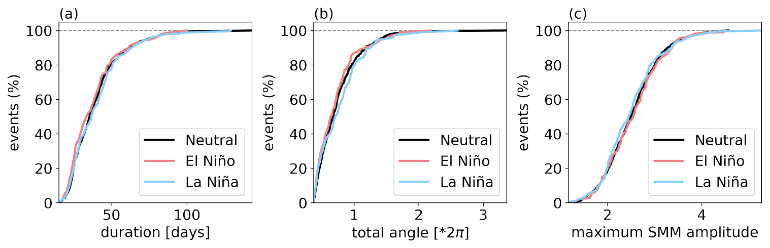
Figure 11 Cumulative probability distribution of the MJO events' durations, total angle covered in (SMM1, SMM2) phase space, and maximum SMM value for simulated events occurring during El Niño, La Niña, and neutral periods. The simulations were forced with data covering the period 1979–2021. The number of events in each sample is reported in Table 1.

8.2.2 Simulations

Finally, we look at the characteristics of MJO events in the model during El Niño, La Niña, and neutral conditions. The results are shown in Fig. 11. For all three MJO characteristics, the cumulative distributions are very similar during El Niño, La Niña, and neutral conditions. We perform a Kolmogorov-Smirnov test to identify whether statistically significant differences exist between the El Niño and La Niña samples for each of the three characteristics. For the duration of MJO events, the test yields a D value (representing the maximum distance between the two curves) of 0.0865 and a p value of 0.4. For the total angles covered, the D value is 0.1307 and the p value 0.05. For the maxima of SMM values, the D value is 0.0858 and the p value 0.4. Hence, none of the three tests provides sufficient evidence to reject the null hypothesis that the two samples come from the same distribution at the 5 % significance level.

We might nonetheless compare the mean and maxima of the three characteristics. To do so, we compute these values in 15 independent simulation runs and determine the mean and standard error of the resulting values. They are summarized in Table 3. On average, we observe slightly smaller mean and maximum durations of MJO events during El Niño compared to other phases of ENSO. We also observe smaller mean and maximum values (on average) of the total angle covered in the SMM phase space during El Niño. No specific tendency is observed for the maxima of SMM values. In all cases, the differences between these values remain small.

8.2.3 Discussion

Comparing observations and simulations, the main difference lies in the fact that, in the simulations, the cumulative distributions of MJO characteristics do not significantly differ under different ENSO conditions (unlike in observations, although limited sample sizes might affect observed patterns). Since the model's forcings S^q and S^θ are significantly different during El Niño and La Niña conditions (Fig. 9), the lack of the model's response to ENSO variability suggests a limitation in the representation of key physical mechanisms governing the MJO–ENSO interactions.

However, some similarities between observations and simulations are still seen when looking at the mean and maxima of MJO characteristics. In both observations and the model, the mean and maximum duration of MJO events are smaller for events occurring during El Niño and larger for events occurring during La Niña (although these differences are relatively small in the model). Similarly, the mean and maximum of the total SMM/RMM angle are smaller during El Niño than during La Niña. On the other hand, no such general tendency is seen for the maximum of SMM/RMM amplitude.

9 Conclusions

We have implemented time-varying observation-based forcing profiles in the MJO stochastic skeleton model. As in previous works (Majda and Stechmann, 2009b, 2011; Thual et al., 2014), the model captures several important features of the MJO, including its phase speed of around 5 m s⁻¹, its flat dispersion relation, its horizontal quadrupole vortex structure (not shown here), and the intermittent generation of MJO events. We found that, when considering planetary scales, the climatology and variance of observed convective activity are in very good agreement. Using an RMM-like index in the model, we were able to objectively identify MJO events and to analyze their characteristics. We find agreement between observations and simulations for the statistics of MJO event durations, total angles covered in SMM/RMM phase space, and maxima of SMM/RMM amplitudes. However, we also show that the model cannot reproduce well the seasonal variations in the MJO occurrences. This could be due to the 3-month averaging of the forcing profiles, which was introduced to ensure the generation of MJO events in the model. This forcing better captures the long-term trends but may have the side effect of blurring the differences between seasons. We note that the number of MJO events generated in the stochastic skeleton model forced with these profiles remains lower than in observations. Future work should investigate the effect of different lengths of time-averaging windows on the frequency of MJO events in the model and on their statistical properties to find the appropriate balance between the large-scale nature of the model ingredients and an appropriate inclusion of relevant short-scale variability.

The model also fails to accurately replicate spatial variations in the MJO properties, such as its starting and ending phases. This limitation may be attributed to the stochasticity in the model, as pointed out in Stachnik et al. (2015). The stochasticity likely has the effect of dampening the geographic dependencies that should arise from the application of zonally varying forcing functions. Further investigation would be required to separate the effects of stochasticity, zonally varying forcing, and non-linearity on the spatial properties of simulated MJO events. To investigate how temporal variability at longer timescales affects the MJO, we evaluated differences in the statistics of the three MJO characteristics mentioned above (duration, angle, and maximum amplitude) under the different phases of ENSO (El Niño, La Niña, and neutral phase) in observations and in the model. We found that while observations might suggest some differences (for instance, a tendency towards shorter-lived MJO events during El Niño), the model does not identify statistically significant differences in duration, total angle covered in SMM phase space, or the maximum SMM value of simulated MJO events between the different ENSO phases.

In conclusion, our results show that the model reproduces well the planetary-scale variability of convective activity and selected characteristics of MJO events, but it does not capture the impact of ENSO phases on these characteristics. This is due to limitations in the structure and ingredients of the skeleton model. More complex interactions such as changes in mean state winds and ocean coupling (Díaz et al., 2023; Suematsu and Miura, 2022; Wei and Ren, 2019; Moser et al., 2024) are needed to capture the interaction between ENSO and the MJO. Further investigation will be needed to determine whether the interannual variability of the model forcing functions impacts other MJO characteristics which have not been studied here, such as the propagation speed of individual events or their longitudinal extent. In order to compute these characteristics as precisely as possible and to make objective comparisons between the model and observations, one will need to implement a method able to track the MJO (e.g., its convective center) in both the simulations and the reanalysis.

Further, while the skeleton model allows us to gain a better understanding of the fundamental physical mechanisms of the MJO, more complexity will likely be needed to fully reproduce the modulation of the MJO by ENSO. In particular, ENSO impacts the extent of MJO penetration in the Pacific Ocean (Pohl and Matthews, 2007; Tam and Lau, 2005; Kessler, 2001). During El Niño years, MJO convective activities often extend eastward beyond the dateline into the Pacific, while during La Niña years, they tend to remain west of the dateline. Pohl and Matthews (2007) also reported that the duration of MJO events is longer during La Niña and shorter during El Niño when events occur from March to May and October to December. Hence, in order to be able to study the effects of ENSO on the MJO, one condition of any model should be that it captures the spatial variability of the MJO as well as its seasonal variations.