the Creative Commons Attribution 4.0 License.
the Creative Commons Attribution 4.0 License.
 | 28 Oct 2020
A method for predicting the uncompleted climate transition process
Pengcheng Yan
Guolin Feng
Wei Hou
Ping Yang
Climate change is expressed as a climate system transiting from the initial state to a new state in a short time. The period between the initial state and the new state is defined as the transition process, which is the key part for connecting the two states. By using a piece-wise function, the transition process is stated approximately (Mudelsee, 2000). However, the dynamic processes are not included in the piece-wise function. Thus, we proposed a method (Yan et al., 2015, 2016) to fit the transition process by using a continuous function. In this paper, this method is further developed for predicting the uncompleted transition process based on the dynamic characteristics of the continuous function. We introduce this prediction method in detail and apply it to three ideal time sequences and the Pacific Decadal Oscillation (PDO). The PDO is a long-lasting El Niño-like pattern of Pacific climate variability (Barnett et al., 1999; Newman et al., 2016). A new quantitative relationship during the transition process has been revealed, and it explores a nonlinear relationship between the linear trend and the amplitude (difference) between the initial state and the end state. As the transition process begins, the initial state and the linear trend are estimated. Then, according to the relationship, the end state and end moment of the uncompleted transition process are predicted.
- Article
(432 KB) - Full-text XML
- BibTeX
- EndNote


A system transiting from one stable state to another in a short period is called abrupt change (Charney and DeVore, 1979; Lorenz, 1963, 1976). The abrupt change system has two or more states (Goldblatt et al., 2006; Alexander et al., 2012); the system swings between these states that are also called equilibrium states in physics. This phenomena is verified in many fields, including biology (Nozaki, 2001), ecology (Osterkamp et al., 2001), climatology (Thom, 1972; Overpeck and Cole, 2006; Yang et al., 2013a, b), brain science (Sherman et al., 1981), etc. The cusp catastrophe has been widely detected in climatology. Many researchers studied the characteristics and early warning signals of the cusp catastrophe (Lenton, 2012; Pierini, 2012; Livina et al., 2012). The latest observed climate change event was a global warning hiatus (Amaya et al., 2018; Kosaka and Xie, 2013; Yang et al, 2017). In Thom's research (1972), seven different kinds of abrupt changes were mentioned. Over the last several decades, many methods have been proposed to identify different kinds of abrupt change (Li et al., 1996), such as the moving t test, Cramer's (Wei, 1999), Mann–Kendall (MK; Goossens and Berger, 1986), Fisher (Cabezas and Fath, 2002), etc. It is noticed that most abrupt change detection methods suggest that the abrupt change is around a turning point. The significant difference between the average values of the two sequences on both two sides of the turning point is defined as the index for measuring the abrupt change. It is difficult for these kinds of methods to detect the transition period of the abrupt change, and it is difficult to identify the abrupt change that occurs at the end of sequence.
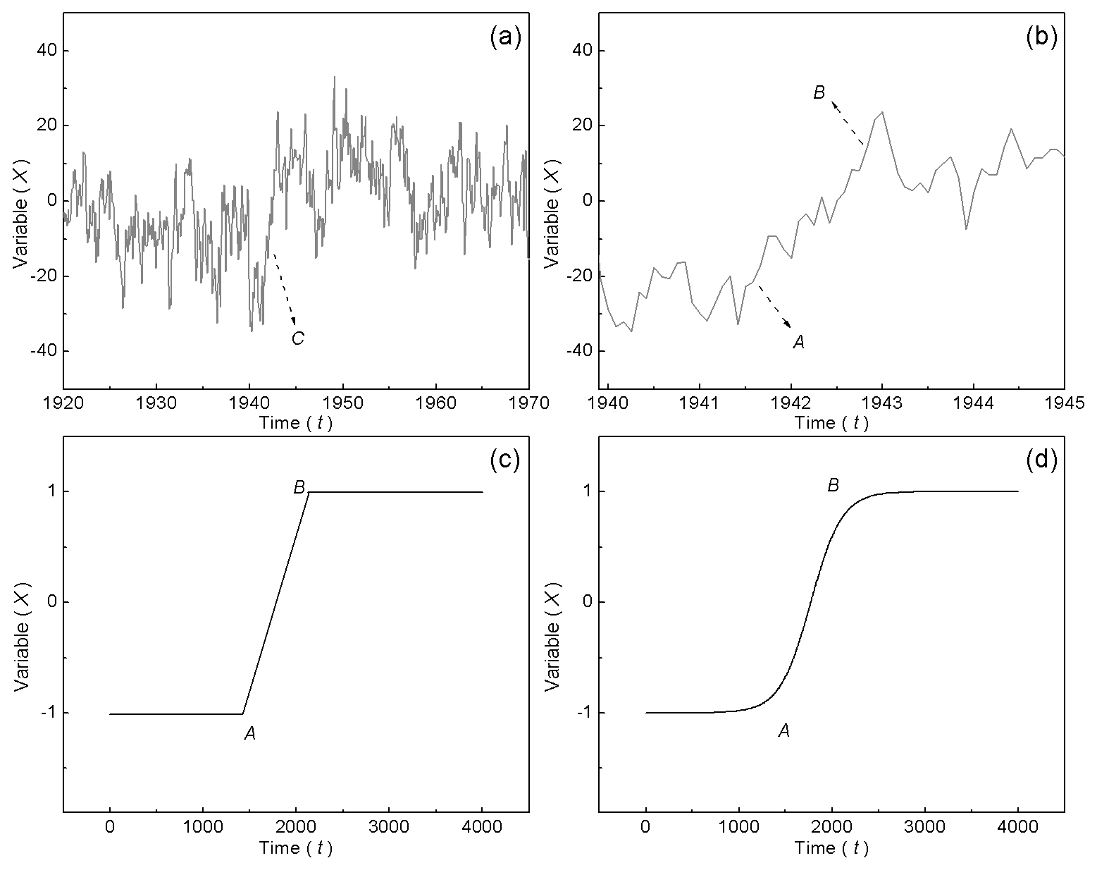
Figure 1Transition process of abrupt change in a real time sequence and an ideal time sequence. (a) The Pacific Decadal Oscillation (PDO) time sequence during 1920–1970. (b) The PDO time sequence during 1940–1945. (c) The transition process presented by piece-wise function. (d) The transition process presented by continuous function.
Mudelsee (2000) studied the abrupt change in a time sequence and illustrated that abrupt change has a duration which can be quantitatively described with a piece-wise (ramp) function. We developed the detection method by using a continuous function to replace the ramp function (Yan et al., 2014, 2015). The new method can confine the beginning and ending points of abrupt change, and it quantitatively describes the process of abrupt climate change, and three parameters are introduced. A quantitative relationship among the parameters is revealed (Yan et al., 2015). The relationship could be used to predict the end moment (state) if the system had left the original state but not yet reached to the new state, which is defined as an uncompleted transition process.

Figure 2(a) The transition processes of the system swinging between different stable states since the parameters are different. (b) The system stays in unstable states. (c) The generalized potential energy function of the system performs differently since the parameters are different. (d) Different segments of the transition process in the ideal time sequence.
In this paper, three ideal time sequences are tested to study the prediction method. The prediction method is also applied to study the climate transition process of the PDO, which is an important signal that reveals climatic variability on the decadal timescale (Mantua et al., 1997; Barnett et al., 1999; Zhang et al., 1997; Yang et al., 2004). Previous studies (Lu et al., 2013; Trenberth and Hurrell, 1994) have indicated that there have been many abrupt changes in the PDO over the past 100 years. Most researches mentioned the climate changes happened in the 1940s and 1970s. During the 1940s, the PDO transited from a high state to a low state, while during the 1970s it did the opposite. All of these changes and their processes were studied in our previous research (Yan et al., 2015, 2016). The climate transition processes were explored clearly. However, we still cannot know when the transition processes finish their increasing or decreasing to a stable state once the transition process has begun. We have developed a new method to predict the end state and the end moment of a transition process based on the quantitative relationship.
It is necessary to describe the transition process quantitatively before the prediction of the uncompleted climate transition process. The detection method by using the logistic model to obtain a transition process is introduced in Sect. 2.1. On the basis of the detection method, the prediction method for studying the uncompleted transition process is further developed in Sect. 2.2.
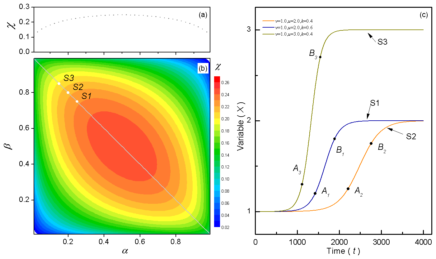
Figure 3The relationship among the parameters α, β, χ and h. (a) Diagonal section of parameter χ in (b) (gray line). (b) Parameter χ with location parameters α and β. (c) Points A and B stay in different positions in the three situations marked as S1, S2 and S3, and the dashed lines connect the two points.
2.1 The detection method of the transition process
The real time sequence changes abruptly as shown in Fig. 1a, and the system jumps to a high state in point C. If the period around point C is observed on a shorter timescale (as shown in Fig. 1b), a transition period is obtained, and it is a part of the original time sequence. In fact, many abrupt changes could be considered to be a transition period with a more detailed view. The transition period was expressed with a ramp function in Mudelsee's research (2000), as shown in Fig. 1c, and the time sequence is divided into three segments, including two equilibrium states and one increasing state. The ramp function is as follows:
where t represents time, and xt represents the system state. Before t1 and after t2, the system stays in the two equilibrium states, namely x1 and x2. Between t1 and t2, the system's states are a straight line. It is noted that the climate system should be smooth and continuous; it is even the sampling sequence that makes it is discrete. We used a continuous function to express this transition period approximately, and we also created a novel method for detecting the transition period (Yan et al., 2015). As shown in Fig. 1d, the transition process is consistent with the continuous evolution of the logistic model, which was created to describe the evolution of population model (May, 1976). The modified logistic model with two changeable equilibrium states is expressed as Eq. (2), in which x represents variable of system state, as follows:
Parameters u and v represent the two equilibrium states, respectively. Parameter u represents the initial state, and parameter v represents the end state. Parameter k represents the switching between different states, and it is defined as the instability parameter. As shown in Fig. 2a, parameters u and v are fixed, and setting k as 0.4 (the dash gray line), the system, increasing to the new state, uses a shorter time than that setting k as 0.3 (the black line). It is noted that if k<0 (as v=1.0, u=2.0 and ), the system decreases from state 2.0 to state 1.0 as the gray line. This states that if the absolute value of k is relatively large, then the transition time of the system is shorter; that is, the more unstable it is (Yan et al., 2016). If parameter k is set large enough, the system collapses and becomes chaotic, as shown in Fig. 2b.
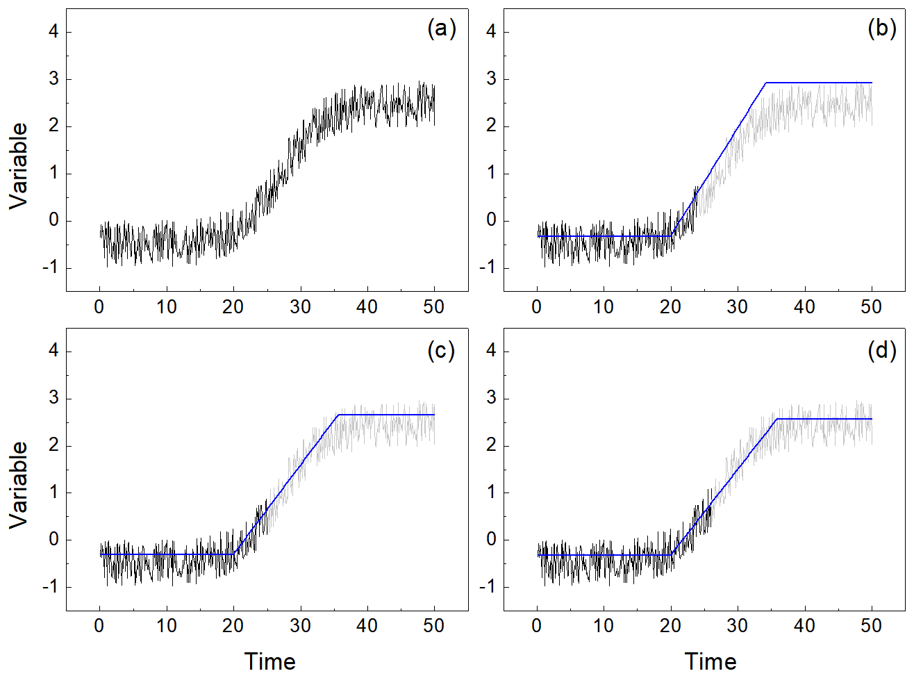
Figure 5The ideal time sequence constructed by the logistic model and random numbers. The x axis represents time, and the y axis represents variable . (a) Completed transition process with 500 moments, uncompleted transition processes (the gray lines) and their prediction results (the blue lines) with (b) 240 moments, (c) 250 moments and (d) 260 moments. The light gray lines are the original entire ideal time sequences.
In Eq. (2), the first derivative of the state variable to time is given, and it is regarded as velocity. The acceleration of the state variable is expressed as the derivative of velocity to time, as shown in Eq. (3). The acceleration of the system is from the external force f(x), which is expressed as . Assuming that the coefficient m is 1, the generalized potential energy (Benzi et al., 1982) is expressed as the integral of the generalized force to the state, as shown in Eq. (4), as follows:
According to Thom's theory (1972), the generalized potential energy of the system described by a quartic function would exhibit a cusp catastrophe in which the system jumps abruptly from one state to a new state.
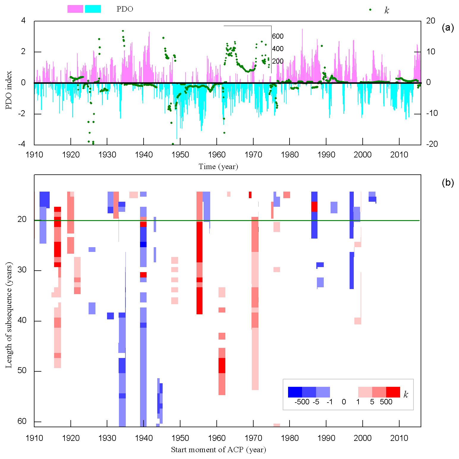
Figure 6Identification of the PDO time sequence and instability parameter k with different subsequence lengths. (a) The histogram represents the PDO time sequence (left y axis), and the green dots indicate the value of parameter k when the subsequence is 20 years (right y axis), where the x axis represents time in year. (b) The start moments of transition processes with different subsequence lengths (the red dots represent increasing processes, and blue dots represent decreasing changes, with deeper colors representing higher values). The green line shows that the value of the subsequence is 20 years. The x axis represents the start moment of abrupt change in year, and the y axis represents the subsequence length in years.
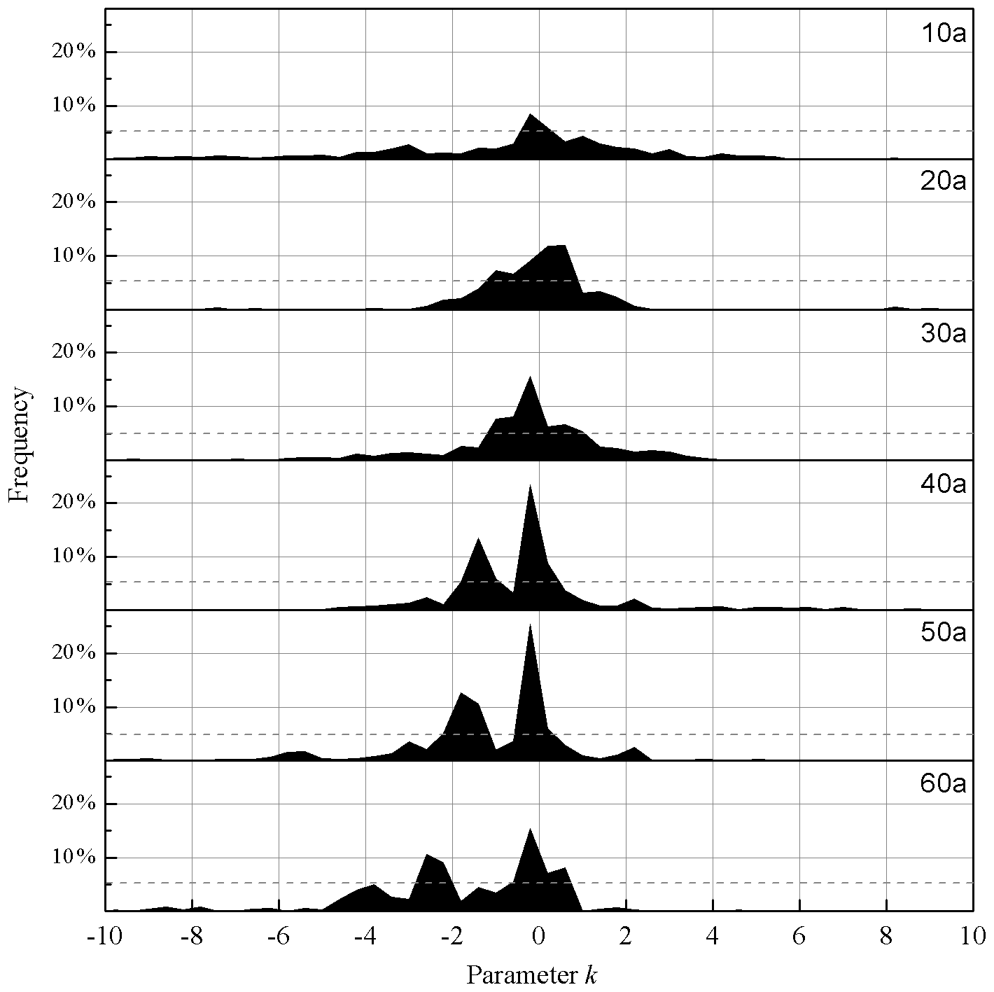
Figure 7Statistical results of instability parameters for different subsequences lengths. The x axis is the value of parameter k, and the y axis is the statistical frequency for the subsequence length of 10a, 20a, 30a, 40a, 50a and 60a.
In Fig. 2c, the potential energy of Eq. (4) is verified as having two states with the lowest energy, and both of them are stable. This bistable structure is common in the climate system (Goldblatt et al., 2006). Therefore, Eq. (2) can be used to describe the abrupt change system, and the parameters of Eq. (2) represent different key factors of the transition period during abrupt change. In order to obtain the values of the parameters, the time sequence is divided into three segments. The first and the third segment represent the two equilibrium states, while the second segment represents the transition process. During the transition process, we define a new parameter h to represent the ratio of system state change to time, and it is called the linear trend. As Eq. (5) shows, the linear trend h can be expressed by two points on the curve, approximately where the two points are A (xa, ta) and B (xb, tb), which are displayed in Fig. 2d, as follows:
In Eq. (6), the values of parameters v and u are calculated. The value of parameter h can be calculated by the regression method (Huang, 1990; Yang et al., 2013a) based on the time sequence of the second segment, where i and xi denote the time and the system state, and and are their averages, respectively. Variables n1, n2 and n3 represent the lengths of the first, the second and the third segment, respectively.
The points A (xa, ta) and B (xb, tb) are also on the curve; thus, we are going to calculate the solution of Eq. (2). Equation (2) is rewritten as Eq. (7), and both sides of the Eq. (7) are integrated as Eq. (8), as follows:
where the variables t0 and x0 represent the initial time and the initial state, respectively. The transition process has been assumed to be linear; thus, we define location parameters α and β as , and xa and xb are expressed as follows:
Substituting Eqs. (8) and (9) into Eq. (7), we have the following:
It is noted that the rightmost part is only related to parameters α and β; then, let it be χ. Then, the relationship of Eq. (10) is rewritten as Eq. (11), as follows:
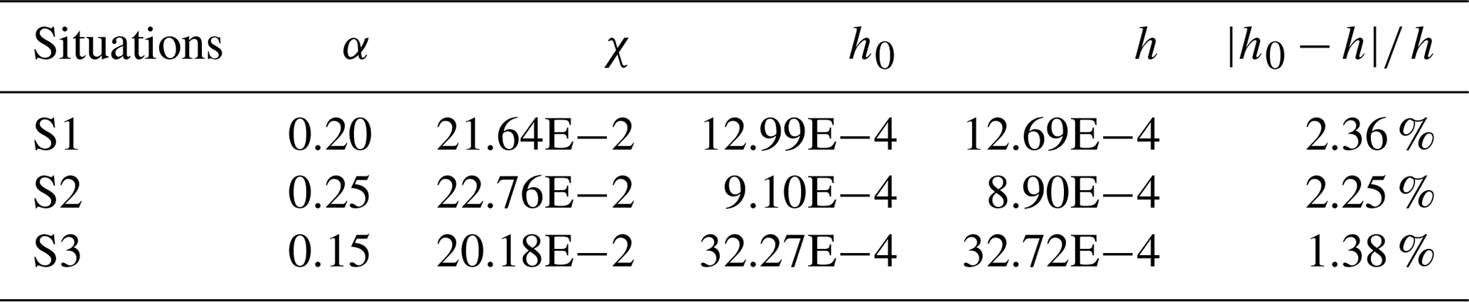
The difference between the initial state v and the end state u and u−v, is called as the amplitude of change. In order to determine the value of parameter χ, the relationship among χ, α and β is displayed in Fig. 3b. The dashed line in Fig. 3a is the profile of the diagonal in Fig. 3b, which represents that the sum of α and β is one. Parameter χ changes little when the location parameter varies in a certain range, as marked with warm color in Fig. 3b. It means that the closer the points (A and B) are to the middle point, the more significant the linear feature is. Then, the process between point A and point B can represent the whole transition process, as shown in Fig. 3c. It is noted that the transition process is symmetrical about the middle point approximately. Thus, we assume that point A and point B are symmetrical about the middle point, and the sum of α and β is one. The change in parameter χ is only related to parameter α (or parameter β), as shown in the diagonals in Fig. 3b (also in Fig. 3a). Parameter χ changes little when parameter α is about 0.2 or larger. In Fig. 3c, three different situations are carried out to study the influence of parameter α on parameter χ. In each situation, points (A and B) are set to be different positions, and their parameters were calculated, respectively, in Table 1. The parameters α are set as 0.20, 0.25 and 0.15, respectively, in three different situations marked with S1, S2 and S3. For S2 and S3, both of the percentages of α that are changing to S1 are 25 %, while the percentages of χ that are changing are only 5.15 % and 6.76 %, respectively, which means the percentage change in χ is much less than α. In addition, linear trends of these three ideal models are calculated according to the points and by regression method, which is marked as h0 in Table 1. The linear trends are also calculated by the values of point A and point B with Eq. (5), which is marked as h in Table 1. It is noted that although the positions of points are different, the trend obtained according to the points is almost the same as that obtained by the regression method. The error percentages are 2.36 %, 2.25 % and 1.38 %, respectively, which means that we do not have to know the exact positions of point A and B (the values of parameters α and β). We can approximate the value of χ. Thus, in the following sections, parameter α is set as 0.2, and parameter χ is 0.2164.
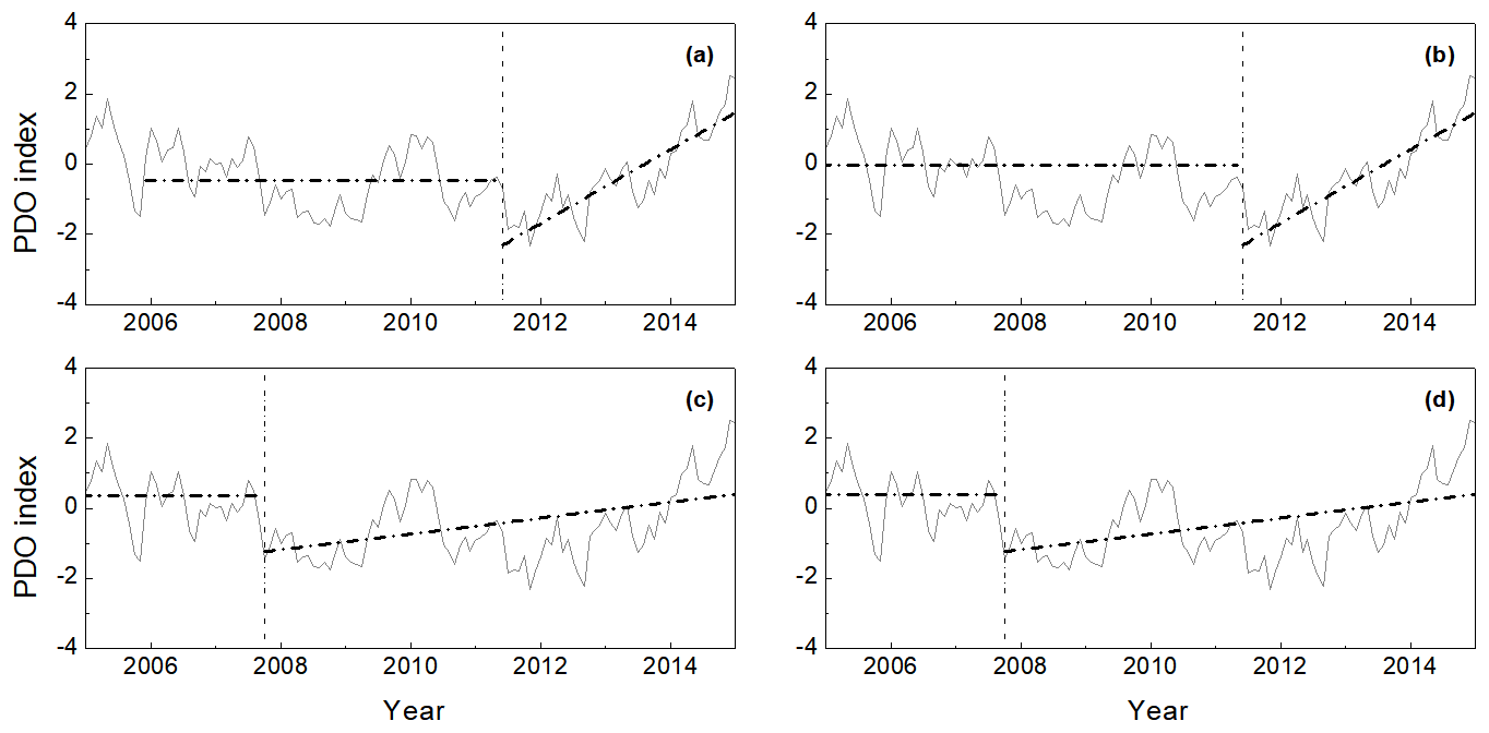
Figure 8The PDO time sequences and the detection of parameters v and h when the subsequence was set as (a) 10 years, (b) 20 years, (c) 30 years and (d) 40 years. The gray lines represent the PDO time sequence. The horizontal dashed lines represent initial states, the sloped dashed lines represent the linear trend lines of the transition process and the vertical dotted lines represent the start moment.
Table 2Parameters v and h have been obtained with different subsequences.
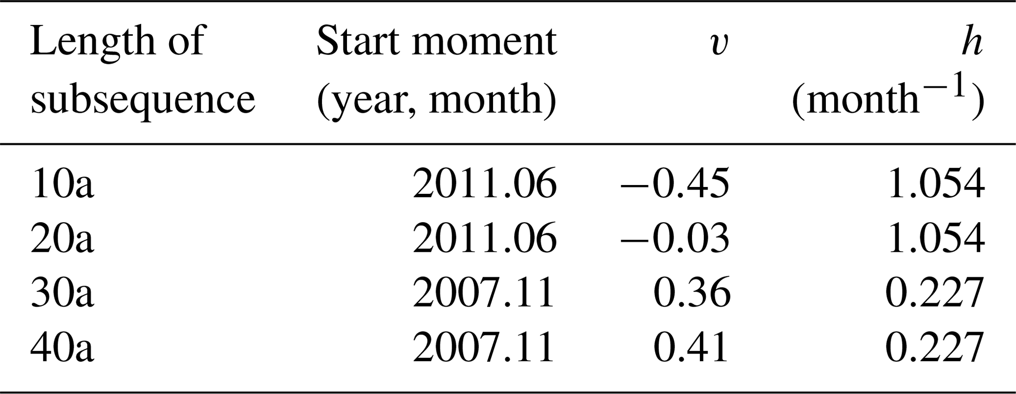
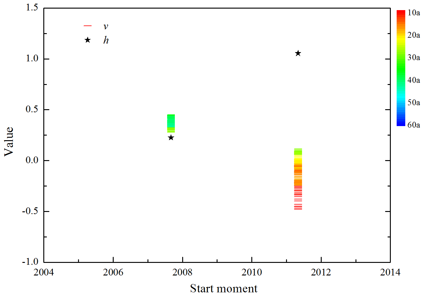
Figure 9The values of the parameters v and k of two transition processes with different lengths of the subsequence. The black stars represent the values of parameter h, and the colorful short bars represent the values of parameter v. The colored bar represents years of the subsequence length from 10 to 60 in intervals of one.
2.2 The prediction method of the transition process
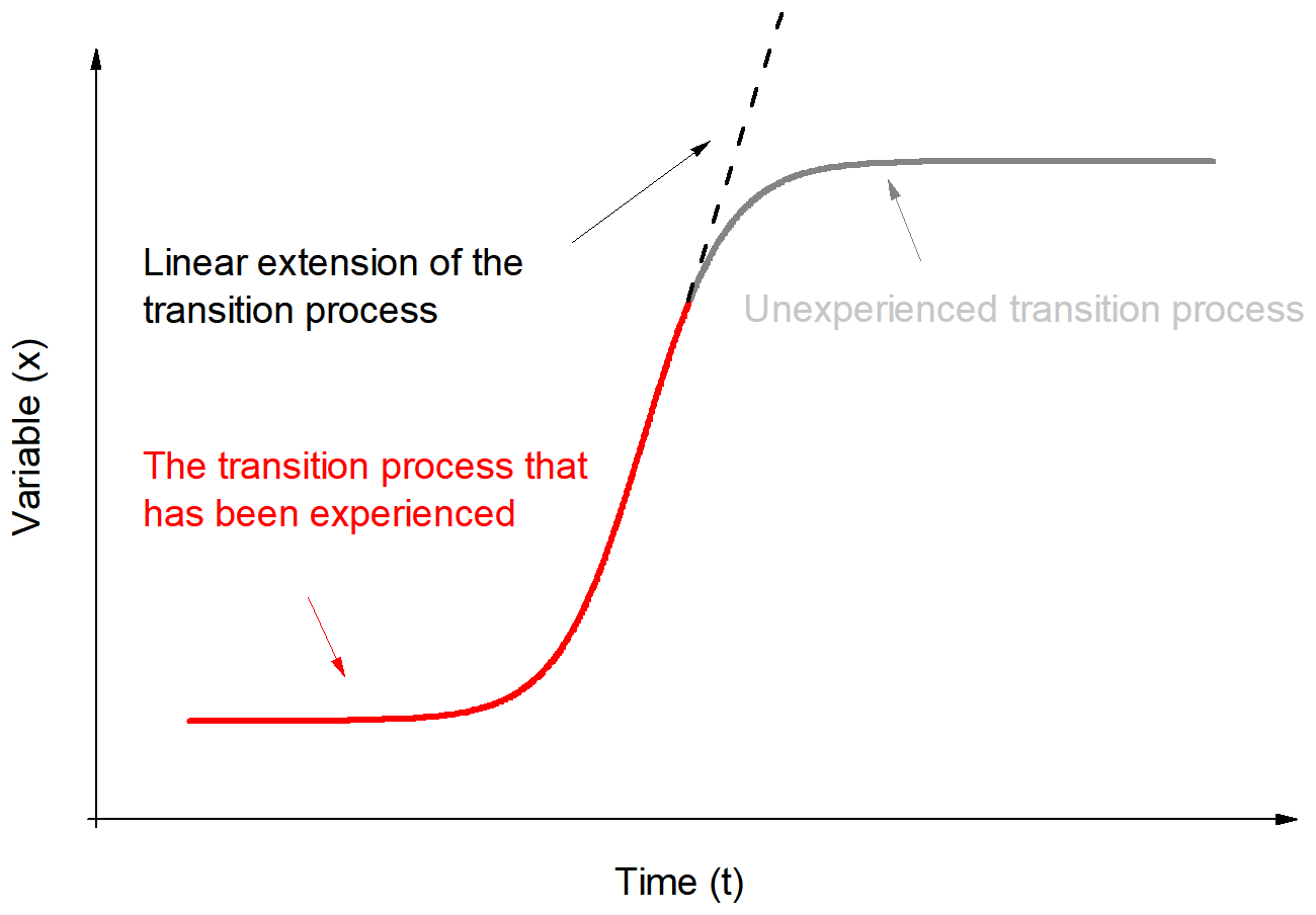
Equation (11) shows the quantitative relationship among the linear trend, instability parameter and amplitude of change. There is a linear relationship between the linear trend and instability parameter, and there is a quadratic function relationship between linear trend and amplitude of change. We revealed this quantitative relationship based on sea surface temperature (Yan et al., 2016). According to this relationship, we are going to develop a new method for predicting the transition process which has not been completed. A brief description about the new method is shown with the schematic diagram in Fig. 4. The red line represents the period which has been experienced, while the gray line represents the period which has not been experienced. Based on the system states which are far away from the original state, a quasi-linear extension of the transition process is established as dashed line. Then, the parameters v and h are obtained by Eq. (6). The instability parameter k represents the stability of abrupt changes in the system, which means that it is related to the system. Its threshold can be estimated by historical data. The parameter u is predicted by Eq. (11), and the end moment can be determined according to the definition of linear trend h.
In order to test the prediction method, an ideal time sequence is constructed by using Eq. (12), which is the sum of the logistic model and random numbers, where ηt represents the random number, as follows:
As seen in Fig. 5, an entire time sequence with 500 moments is shown in Fig. 5a and three other time sequences with different lengths are shown in Fig. 5b, c and d, respectively. The parameters v, u and k of the logistic model are set as −1.0, 2.0 and 0.1 for the ideal time sequence, and the random number is limited to 0–1. The parameters v and h are obtained by the regression method before making the prediction. It has to be noted that in this ideal time sequence there is just one abrupt change, which means that we have no way of obtaining the value of the parameter k by counting other abrupt changes. Thus parameter k is given directly, and the prediction of the end state (moment) is drawn in Fig. 5b, c and d. For the entire time sequence, there are 500 moments, as shown in Fig. 5a. In Fig. 5b, only 240 moments are given, and the other moments are unknown. Then, we obtain parameters v and h by the regression method. The parameter u is calculated with Eq. (6). The blue line represents the prediction result. The transition process would end in moment 342, with the end state value of 2.92. In Fig. 5c, the end moment and end state are predicted to be 356 and 2.65, respectively, when the time sequence is given 250 moments. In Fig. 5d, the time sequence is given 260 moments. The end moment and end state are predicted to be 359 and 2.58, respectively. The predicted end moment and the predicted end state are basically consistent with the original time sequences. However, the average absolute prediction errors of the three time sequences are 0.37, 0.27 and 0.26, respectively. When the length of the sequence is 240, the prediction state is overestimated, and the average absolute prediction error is 0.37. With the length of the system experiencing expansion, the prediction error decreases. The prediction states are very close to the original states when the length is 260. Therefore, in the actual prediction, we hope that the transition process has been experienced for a long enough time, which will help us to predict accurately.
In order to test the validity of this prediction method in a real climate system, we apply this method to predict the uncompleted transition process of the PDO. The PDO index data used are from website of the National Oceanic and Atmosphere Administration (NOAA; https://psl.noaa.gov/gcos_wgsp/Timeseries/Data/pdo.long.data, last access: October 2020). The time period from January 1900 to November 2015 is studied as the training data, and the time period from December 2015 to April 2017 is used as the test data. During the following research, a transition process starting from 2011 is studied. According to the prediction method, several parameters have to be determined in advance. We first determine parameter k.
3.1 Threshold of parameter k
Parameter k characterizes the stability of the system during climate change, which means that we can estimate the value of parameter k by counting all abrupt changes of the PDO index. The histogram in Fig. 6a shows the PDO time sequence from January 1900 to November 2015, and it shows that the PDO went through several transition processes. The green dots in Fig. 6a are parameter k when the subsequence length takes 20 years. In the early 1940s and late 1970s, there were two main transitions of the PDO. The absolute value of the parameter k is large, which means that the system is much more unstable during these two transition processes. In the 1940s, the PDO transits from a positive phase to a negative phase and k<0, whereas the situation in the 1970s is the opposite. Figure 6b shows more kvalues corresponding to the different subsequence lengths (as indicated by y axis, the variation range of the subsequence is 15–60 years, with an interval of 1 year). The x axis represents the start moment, and the locations of the dots indicate the start moments for the corresponding subsequence lengths. In particular, the blue dots represent parameter k as being negative, and the red dots represent it as being positive. There are more dots when the subsequence is short. This is because, when the length of subsequence is short, the amplitude is also often small, which leads to more transition processes being detected. When the length of the subsequence reaches or exceeds 50 years, the transition processes mainly begin in the 1940s and 1970s. Such climate changes are also investigated in the previous research (Shi et al., 2014). The transition processes in these two periods correspond to large k values, which means that these two transition processes are more unstable than others. The small figure in Fig. 7a shows that the k values (marked with green dots) are more than 100 during 1960–1970 when the length of subsequence is 20 years. The frequencies of parameter k values, when the length of subsequence are 10, 20, 20, 40, 50 and 60 years, respectively, are displayed in Fig. 7. It is noted that some of the values of parameter k are so large that their frequencies are almost zero, which makes counting them unnecessary. The frequencies of the k values which belong to −10 to 10 are shown in Fig. 7. By considering the frequency which is bigger than 5 % as a peak, there is only one peak when the length of subsequence is 10 years. Most of the k values are concentrated around zero, which means that the transition processes detected are stable. For the situations in which the lengths of subsequences are 20 and 30 years, there is mainly one peak, and it is near zero. When the lengths of subsequences are more than 30 years, there are mainly two peaks. One is near zero, and another is much less than zero. Thus, the much more unstable transition processes are detected when the lengths of subsequences are large. From the perspective of the k threshold values, the k values in the range of [−10, 10] account for 63.90 %, 70.64 %, 77.00 %, 90.05 %, 93.69 % and 89.90 % of all k values for which the lengths of the subsequences are 10, 20, 30, 40, 50 and 60 years, respectively. They are 55.64 %, 67.52 %, 73.99 %, 83.45 %, 85.46 % and 84.82 % for the range of [−5, 5] and 35.64 %, 62.22 %, 59.36 %, 68.28 %, 66.25 % and 47.55 % for the range of (−2, 2). In the following studies, the k values are mainly considered to be in the range of [−2, 2].

Figure 10Variation end state and end moment, with the initial state parameter v (horizontal ordinate) and instability parameter k (vertical coordinate). The red line on the right-hand side shows the probability distribution of instability parameter k.
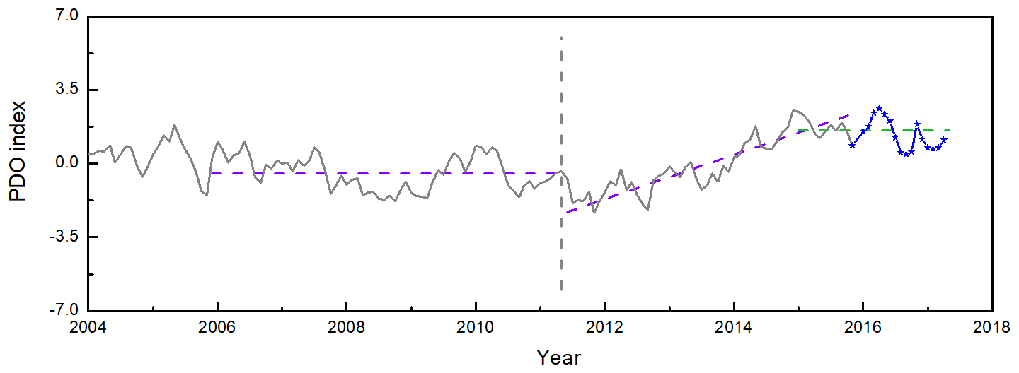
Figure 11Prediction of the PDO index. The gray line represents the PDO index before 2015, the blue line represents the PDO index after 2015, the gray dashed line represents the start moment and end moment, the purple dashed lines represent the initial state and the linear trend line and the green line represents the prediction end state.
3.2 Values of the initial state v and linear trend h
We use the method proposed in Sect. 2.2 to analyze the transition processes of the PDO. With different lengths of subsequences, three climate changes are detected to start from 1976, 2007 and 2011, respectively. In Fig. 8, the transition processes starting from 2007 and 2011 are shown, while the transition process starting from 1976 has not been shown. In Table 2, parameters v and h are obtained by regression method for the transition processes starting from 2007 and 2011. When the length of subsequence is 10 or 20 years, only the transition process starting from 2011 is detected, as shown in Fig. 8a and b. The parameter v is calculated with the sequence before 2011. Then, the linear trend parameter h is calculated with the segment after 2011. For the transition process starting from 2011, the values of initial state were detected to be −0.45 and −0.03 when the length of subsequence is 10 or 20 years, respectively, and both the linear trends are 1.054 month−1. When the lengths of subsequences are set as 30 and 40 years, the transition process begins in 2007, as shown in Fig. 8c and d, and the values of the initial state are 0.36 and 0.41, respectively, with an linear trend of 0.227 month−1. When we detect the transition process in a subsequence, the percentile threshold method (Huang, 1990) is used. Then, a transition process in the subsequence is detected (Yan et al., 2015, 2016). The change with the largest amplitude will be detected. The start moment of the transition process is identified to be 2011, as shown in Table 2.
In Fig. 8, it is noted that the PDO time sequence is leaving the stable state from the start moment. The transition process occurs over a period of time, which is called the transition process. When the transition process has not finished, it appears to be increasing. In order to detect whether there are other transition processes, we changed the length of the subsequences to yearly intervals. That is, the subsequence length is set as 10, 11, 12, …, up to 60 years. Then, the initial state v and the linear trend h of these transition processes are obtained, as shown in Fig. 9. When the subsequence length is set at less than approximately 40 years, the transition processes are detected only twice. One began in 2007, and the other began in 2011. The value of parameter h is nearly unchangeable for each transition process, while the value of parameter v changes when the length of the subsequence is different. In particular, the transition process starting from 2007 is detected for the subsequences of about 30–40 years, and the value of parameter v is in the range of [0.28, 0.45]. The transition process starting from 2011 is detected for subsequences of about 10–30 years, and the value of parameter v increases as the length of the subsequence increases, whereas the variation range in parameter v is [−0.48, 0.12], which is significantly different from the situation of the transition process starting from 2007.
3.3 Prediction of the uncompleted transition process beginning in 2011
After the threshold ranges for parameters k, v and h are determined according to the quantitative relationship, we can calculate the end state and the end moment of the transition process. Using the transition process in 2011 as an example, we study the end state and end moment for the PDO index transition process. According to the research results that are presented in Sects. 3.1 and 3.2, the parameter is in this transition process, and the threshold range of parameter k is determined to be [0, 2]. The range of parameter v is determined to be [−0.48, 0.12], and the variation situation of parameter u and end moment with parameters k and v are shown in Fig. 10. The results indicate that the threshold range of parameter u for the ending state is [1, 7], and the time range of the ending moment is [2013, 2017]. According to the probability of parameter k, the end moment of this transition process is about 2015, and after that time, the sequence stops increasing, approaching a stable state with value of 1.6.
In Fig. 11, a sketch map is displayed to briefly explain how the prediction method works. The PDO time sequence is displayed as a black line. The period during 2006–2011 is detected as the initial state, and a transition process is increasing from this initial state. It is possible to know whether the increasing process has been completed or not. Based on the linear regression method, the initial state and the linear trend are obtained and are shown as purple dashed lines. Then, by the method proposed in Sect. 2.2, all possible end states of this transition process are obtained with Eq. (9), as shown in Fig. 10, and the most likely end state is marked as a green dashed line. Unlike the uncompleted transition process of the ideal experiment, the transition process is completed in about 2015 since we detected the PDO change in 2016. This transition process started from 2011 and ended in 2015. The initial moment and the end moment are marked as black dashed lines. However, we are still not sure whether the PDO finished this transition process completely or not for it appears at the end of the sequence. Many statistical methods are not accurate for detecting both ends of the sequence. Thus, the real PDO sequence during 2016–2017 is added to the end of the PDO time sequence. The PDO value from 2015 to 2017 is almost unchanged, which is consistent with the predicted result.
A novel method had been proposed for identifying the transition process of climate change in our previous research. By defining the initial state parameter v, linear trend parameter h, end state parameter u and instability parameter k, a quantitative relationship among these parameters was revealed. Based on the relationship, we developed a method for studying uncompleted transition processes. The method is applied to predict ideal time sequences and the PDO time sequence. In the ideal experiments, three different time sequences with different lengths were constructed. Based on the initial state and the linear trend which the system experienced and the given parameter, the end state and end moment of the transition process are predicted. The prediction result matches the ideal time sequence well. For the PDO time sequence, a transition process beginning in 2011 was taken to test the prediction method. The end moment of this transition process was predicted to be 2015, which is consistent with the real time sequence.
In this prediction method, the quantitative relationship among the parameters characterizing the transition process is vital. According to the segment of the transition process which has occurred, we determine the parameters and predict the end moment and the end state. In fact, this is also an extrapolation method. It is noted that the uncompleted climate change we studied is closed to the end of the sequence. Due to the lack of enough data, it is difficult to study the end of time sequence by using other statistical methods.
We analyzed the transition process of the PDO using data from the National Oceanic and Atmospheric Administration (NOAA), available at: https://psl.noaa.gov/gcos_wgsp/Timeseries/Data/pdo.long.data (last access: October 2020; Mantua et al., 1997).
PY and GF contributed to the conception of the study. PY performed the data analyses and wrote the manuscript. WH and PY helped preform the analysis with constructive discussions.
The authors declare that they have no conflict of interest.
We thank the three anonymous reviewers for their valuable suggestions.
This research has been supported by the National Key Research and Development Program of China (grant no. 2018YFE0109600), the National Natural Science Foundation of China (grant nos. 41875096, 41775078 and 41675092), and the Northwest Regional Numerical Forecasting Innovation Team (grant no. GSQXCXTD-2017-02), and the Meteorological scientific research project of Gansu Meteorological Bureau (grant no. MS201914).
This paper was edited by Ana M. Mancho and reviewed by three anonymous referees.
Alexander, R., Reinhard, C., and Andrey, G.: Multistability and critical thresholds of the Greenland ice sheet, Nat. Clim. Change, 2, 429–432, 2012.
Amaya, D. J., Siler, N., Xie, S. P., and Arthur, J. M.: The interplay of internal and forced modes of Hadley Cell expansion: lessons from the global warming hiatus, Clim. Dynam., 51, 305–319, https://doi.org/10.1007/s00382-017-3921-5, 2018.
Barnett, T. P., Pierce, D. W., Latif M., and Dietmar, D.: Interdecadal interactions between the tropics and midlatitudes in the Pacific basin, Geophys. Res. Lett., 26, 615–618, 1999.
Benzi, R., Parisi, G., Sutera, A., and Vulpiani, A.: Stochastic resonance in climatic change, Tellus, 34, 10–16, 1982.
Cabezas, H. and Fath, B. D.: Towards a theory of sustainable systems, Fluid Phase Equilibria, 3, 194–197, https://doi.org/10.1016/S0378-3812(01)00677-X, 2002.
Charney, J. G. and Devore, J. G.: Multiple flow equilibria in the atmosphere and blocking, J. Atmos. Sci., 36, 1205–1216, 1979.
Goldblatt, C., Lenton, T. M., and Watson, A. J.: Bistability of atmospheric oxygen and the Great Oxidation, Nature, 443, 683–686, https://doi.org/10.1038/nature05169, 2006.
Goossens, C. and Berger, A.: Annual and Seasonal Climatic Variations over the Northern Hemisphere and Europe during the Last Century, Ann. Geophys., 4, 385–400, https://doi.org/10.1016/0040-1951(86)90317-3, 1986.
Huang, J. Y.: Meteorological Statistical Analysis and Prediction, China Meteorological Press, Beijing, 28–30, 1990.
Kosaka, Y. and Xie, S. P.: Recent global-warming hiatus tied to equatorial Pacific surface cooling, Nature, 501, 403–407, https://doi.org/10.1038/nature12534, 2013.
Lenton, T. M.: Arctic Climate Tipping Points, Ambio, 41, 10–22, 2012.
Li, J. P., Chou, J. F., and Shi, J. E.: Complete detection and types of abrupt climatic change, J. Beijing Meteorol. College, 1, 7–12, 1996.
Livina, V. N., Ditlevsen, P. D., and Lenton, T. M.: An independent test of methods of detecting system states and bifurcations in time-series data, Phys. A-Stat. Mech. Appl., 391, 485–496, 2012.
Lorenz, E. N.: Deterministic nonperiodoc flow, J. Atmos. Sci., 20, 130–141, https://doi.org/10.1175/1520-0469(1963)020<0130:Dnf>2.0.Co;2, 1963.
Lorenz, E. N.: Nondeterministic theories of climatic change, Quaternary Res., 6, 495–506, https://doi.org/10.1016/0033-5894(76)90022-3, 1976.
Lu, C. H., Guan, Z. Y., Li, Y. H., and Bai, Y. Y.: Interdecadal linkages between Pacific decadal oscillation and interhemispheric oscillation and their possible connections with East Asian Monsoon, Chin. J. Geophys., 56, 1084–1094, https://doi.org/10.1002/cjg2.20012, 2013.
Mantua, N. J., Hare, S., Zhang, Y., John, W., and Robert, F.: A Pacific Interdecadal Climate Oscillation with Impacts on Salmon Production PDO, B. Am. Meteorol. Soc., 78, 1069–1079, https://doi.org/10.1175/1520-0477(1997)078<1069:Apicow>2.0.Co;2, 1997.
May, R. M.: Simple mathematical models with very complicated dynamics, Nature, 261, 459–467, https://doi.org/10.1038/261459a0, 1976.
Mudelsee, M.: Ramp function regression: a tool for quantifying climate Transitions, Comput. Geosci., 26, 293–307, https://doi.org/10.1016/s0098-3004(99)00141-7, 2000.
Newman, M., Alexander, M. A., Ault, T. R., and Cobb, K. M.: The Pacific Decadal Oscillation, Revisited, J. Climate, 29, 4399–4427, https://doi.org/10.1175/Jcli-D-15-0508.1, 2016.
Nozaki K.: Abrupt change in primary productivity in a littoral zone of Lake Biwa with the development of a filamentous green-algal community, Freshwater Biol., 46, 587–602, 2001.
Osterkamp, S., Kraft, D., and Schirmer, M.: Climate change and the ecology of the Weser estuary region: Assessing the impact of an abrupt change in climate, Clim. Res., 18, 97–104, 2001.
Overpeck, J. T. and Cole, J. E.: Abrupt change in earth's climate system, Annu. Rev. Environ. Resour., 31, 1–31, https://doi.org/10.1146/annurev.energy.30.050504.144308, 2006.
Pierini, S.: Stochastic tipping points in climate dynamics, Phys. Rev. E, 85, 027101, https://doi.org/10.1103/PhysRevE.85.027101, 2012.
Sherman, D. G., Hart, R. G., and Easton, J. D.: Abrupt change in head position and cerebral infarction, Stroke, 12, 2, https://doi.org/10.1161/01.Str.12.1.2, 1981.
Shi, W. J., Tao, F. L., Liu, J. Y., Xu, X. L., Kuang, W. H., Dong, J. W., and Shi, X. L.: Has climate change driven spatio-temporal changes of cropland in northern China since the 1970s?, Clim. Change, 124, 163–177, https://doi.org/10.1007/s10584-014-1088-1, 2014.
Thom, R.: Stability Structural and Morphogenesis, Sichuan Education Press, Sichuan, 1972.
Trenberth, K. E. and Hurrell, J. W.: Decadal atmosphere-ocean variations in the Pacific, Clim. Dynam., 9, 303–319, https://doi.org/10.1007/Bf00204745, 1994.
Wei, F. Y.: Modern Climatic Statistical Diagnosis and Forecasting Technology, China Meteorological Press, Beijing, 1999.
Yang, P., Xiao, Z. N., Yang, J., andc Liu, H.: Characteristics of clustering extreme drought events in China during 1961–2010, Acta Meteorol. Sin., 27, 186–198, 2013a.
Yang, P., Ren, G. Y., and Liu, W.: Spatial and temporal characteristics of Beijing urban heat island intensity, J. Appl. Meteorol. Climatol., 52, 1803–1816, 2013b.
Yang, P., Ren, G. Y., and Yan, P. C.: Evidence for a strong association of short-duration intense rainfall with urbanization in the Beijing urban area, J. Climate, 30, 5851–5870, 2017.
Yan, P. C., Feng, G. L., Hou, W., and Wu, H.: Statistical characteristics on decadal abrupt change process of time sequence in 500 hPa temperature field, Chin. J. Atmos. Sci., 38, 861–873, 2014.
Yan, P. C., Feng, G. L., and Hou, W.: A novel method for analyzing the process of abrupt climate change, Nonlin. Processes Geophys., 22, 249–258, https://doi.org/10.5194/npg-22-249-2015, 2015.
Yan, P. C., Hou, W., and Feng, G.: Transition process of abrupt climate change based on global sea surface temperature over the past century, Nonlin. Processes Geophys., 23, 115–126, https://doi.org/10.5194/npg-23-115-2016, 2016.
Yang, X. Q., Zhu, Y. M., Xie, Q., and Ren, X. J.: Advances in studies of Pacific Decadal Oscillation, Chin. J. Atmos. Sci., 28, 979–992, 2004.
Zhang, Y. J., Wallace, M., and Battisti, D. S.: Enso-like interdecadal variability: 1900–93, J. Climate, 10, 1004–1020, https://doi.org/10.1175/1520-0442(1997)010<1004:Eliv>2.0.Co;2, 1997.