Bayesian data selection to quantify the value of data for landslide runout calibration

The reliability of physics-based landslide runout models depends on the effective calibration of their parameters, which are often conceptual and cannot be physically measured. Bayesian methods offer a robust framework to incorporate uncertainties in both model and observations into the calibration process. Therefore, they are increasingly used to calibrate physics-based landslide runout models. However, the reliability of Bayesian calibration in its practical application to real-world landslide events depends on the availability and quality of observational data – from aggregated post-event measurements such as impact area to time-resolved data such as force time histories. Despite this, systematic investigation of the influence of observational data on the Bayesian calibration of landslide runout models has been limited.

We propose quantifying the impact of observational data on calibration outcomes by measuring the information gained during the calibration process using an information-theoretic measure called Kullback-Leibler (KL) divergence. Building on this, we present a unified Bayesian data selection workflow to identify the most informative dataset for calibrating a given parameter. The workflow runs parallel calibration routines across available observation datasets. It then computes the information gained relative to the observations by calculating the KL divergence between prior and posterior distributions and selects the dataset that yields the highest KL divergence.

We demonstrate our workflow using an elementary landslide runout model, calibrating friction parameters with a diverse set of synthetic observations to evaluate the impact of data selection on parameter calibration. Specifically, we compare and quantify the information gained from calibration routines using observations that differ in information content (runout distance versus maximum velocity), granularity (aggregated versus time series data), and temporal characteristics (resolution and length of the velocity time series). The insights from this study will optimize the use of available observations for calibration and guide the design of effective data acquisition strategies.

1 Introduction

Landslides are a significant natural hazard, with their frequency and intensity increasing as climate change makes extreme weather patterns more likely (Petley, 2012; Perkins, 2012; Wang et al., 2023). Understanding and predicting landslide runout behavior – how far and fast landslides travel (Xu et al., 2019) – is therefore crucial for impact-based risk and hazard assessment (Willenberg et al., 2009; Froese et al., 2012) and for the development of effective mitigation strategies (Mancarella and Hungr, 2010; Hübl et al., 2009). To this end, we use physics-based runout models, which are adept at capturing the bulk behavior of landslides, an essential objective in runout forecasting (McDougall, 2017). A wide variety of physics-based computational runout models are available, and they can be broadly classified on the basis of the fidelity level and flow characteristics accounted for, the underlying rheological relationships, and the computational methods used to solve them. McDougall (2017) and Trujillo-Vela et al. (2022) compiled a collection of selected computational models. Most of these landslide runout models are semi-empirical due to the absence of universal constitutive laws governing the complex and diverse phenomena involved in landslides (Pastor et al., 2012). Consequently, these models rely on empirical constitutive relations rather than mechanistic subscale formulations representing microscale behavior. This implies the presence of conceptual parameters (Iverson, 2003) that cannot be physically measured and thus must be calibrated based on the re-analyses of past landslide events. By calibration, we refer to the process of inferring model parameters from observational data. The applicability of such calibrated computational models is therefore limited to the physical regime covered by the available calibration data and offers little insight into the complex micromechanical properties of real landslides (McDougall, 2017). However, their ability to reproduce the bulk behavior of landslides makes them a pragmatic choice to analyze the landslide runout behavior (Hungr, 1995) and allows their use as operational tools in hazard mitigation.

Computational calibration methods play an essential role in the model-based prediction tool chain, particularly in landslide runout modeling. In the past, landslide runout models were predominantly calibrated using deterministic methods, traditionally based on subjective trial and error choices (Hungr and McDougall, 2009). These deterministic methods are limited by equifinality and non-uniqueness issues (McMillan and Clark, 2009) and do not offer a robust framework to handle multiple uncertainties, for instance due to model and data errors, involved in the calibration process (Barros et al., 2009). In contrast, probabilistic methods effectively address these limitations by aiming for the probability distributions of the parameters rather than a deterministic estimate. Bayesian methods represent initial parameter uncertainty with a prior distribution, which is updated based on observational data to yield a posterior distribution reflecting the reduced uncertainty. This process thus offers a comprehensive framework to explicitly handle the various uncertainties involved in calibrating computational models that include conceptual parameters.

Recently, Bayesian methods have attracted significant interest from the geohazard research community. For example, Fischer et al. (2020) and Heredia et al. (2020) calibrated the rheological parameters of a snow avalanche propagation model employing a Bayesian approach. Aaron et al. (2019) applied this approach to calibrate a landslide runout model and compared its performance with a deterministic parameter identification algorithm. Furthermore, Moretti et al. (2020) inverted landslide characteristics using seismic data within a Bayesian framework. One significant finding in these studies that is also known from other application fields is that applying Bayesian methods typically entails a significant computational burden because of the large number of so-called forward computational model evaluations required. This high computational cost is the primary limitation of Bayesian methods in their practical applications (Aaron, 2017; Brezzi et al., 2016). A recent trend in simulation for computationally costly high-throughput tasks is, therefore, to train non-intrusive surrogate models that aim at substituting the original simulation model with a fast-to-evaluate alternative that, for example, can be utilized for uncertainty quantification (Yildiz et al., 2023). Zhao and Kowalski (2022) leveraged surrogates based on Gaussian Process (GP) emulation to develop a computationally feasible Bayesian calibration workflow, while Navarro et al. (2018) adopted a similar approach using the polynomial chaos expansion ansatz to build surrogates.

Although integrating fast-evaluating surrogates into the calibration workflow alleviates the computational burden associated with Bayesian calibration methods, this addresses only one part of the challenge. Effective calibration essentially relies on reducing the discrepancy between model predictions and observational data (Cotter, 2024; Aaron et al., 2022). Two important factors contribute to this discrepancy: (i) the potential inadequacy of the model to capture the real-world process to be predicted, and (ii) the innate measurement uncertainties within the observational data. Model inadequacy and its impact on the efficacy of the calibration process have been addressed, for example, in the work of Kennedy and O'Hagan (2001), Heo et al. (2015), and Xu and Valocchi (2015).

The measurement uncertainty in the observational data affects the uncertainty of the predicted landslide runout when those data are integrated into the computational calibration method underlying the model-based prediction tool chain. Methods for handling measurement-related uncertainty are well established. These typically involve incorporating a statistical noise model, such as a Gaussian distribution, into the calibration process. Hyperparameters such as mean and standard deviation are assumed heuristically or inferred along with the model parameters (Zhao and Kowalski, 2022; Heredia et al., 2020) from the data. Several studies use this approach to assess the influence of uncertainty in the observational data on the calibration outcomes (Aaron et al., 2019). A typical outcome is, hence, insight into the acceptable measurement uncertainty to guarantee a specific quality of the calibration result, which in turn dictates the reliability of the computational model predictions.

However, it is seldom considered that different types of observational data, such as an outline of the area affected by a landslide versus a localized measurement of its deposition height, result in markedly different calibration results. This observation holds even if identical Gaussian noise assumptions are being used. Such differences indicate that the choice of observational data not only plays a critical role in shaping calibration outcomes but also constitutes a lever to improve the quality of calibration outcomes. This insight is echoed in the work of Zhao and Kowalski (2022), who found that remarkably localized spatial data, such as maximum velocities or deposit heights, provided better constraints for friction coefficients than aggregated data like deposit volume and impact area. Moretti et al. (2020) made similar observations and found that force time history data was more adept at inverting the characteristics of the landslide than static data such as deposit area or runout distance. This is a surprising result since it strongly seems to indicate that even if we are ultimately interested in predicting the impact area, physics-based computational landslide models should not necessarily be calibrated only based on the impact area of past results, but should also take into consideration local information such as a measurement of the deposition height at a specific location.

Any systematic investigation of this effect requires an approach that quantifies the value of concrete choices of observational data and lays the foundation for systematically assessing the value-add of specific choices of observational data on the calibration outcome and, eventually, the predictive quality of the computational prediction pipeline. Such methods are currently unavailable, yet would be highly relevant to the geohazard community since observational data are often sparse due to logistical and financial constraints. Gaining clearer insight into how different observations influence calibration outcomes could support more efficient use of available data and guide the design of smarter data acquisition strategies. Similar ideas have been followed in other fields. Kavetski et al. (2011) examined the impact of data resolution on the inference of hydrological model parameters using data from an experimental basin, while Li et al. (2010) and Cui et al. (2015) investigated the effect of dataset length on the calibration of the hydrological model in data-limited catchments. In building energy modeling, Heo et al. (2015) studied the role of data quantity and quality in Bayesian calibration of the EnergyPlus model (U.S. Department of Energy, 2024). However, even these studies qualitatively compare the calibration outcomes and do not attempt to quantify the impact, which would help us to optimize data acquisition.

We can assess the impact of observations on the Bayesian calibration outcome by examining the resulting posterior distributions since they represent the uncertainty reduced during calibration. While Zhao and Kowalski (2022) reported variation in calibration outcomes across observational datasets by qualitatively comparing the corresponding posterior distributions, Moretti et al. (2020) analyzed this variation using the modes of the posterior distributions. However, neither of these approaches captures the inherent pathway by which observations influence Bayesian calibration: updating prior beliefs with information to obtain the posterior distribution. We therefore measure this information gained during calibration to quantify the impact of observational data on calibration outcomes. To this end, we employ the Kullback-Leibler (KL) divergence, an information-theoretic concept, to compare probability distributions. Specifically, it measures the information lost when approximating a probability distribution relative to the true distribution. Thus, we quantify the information gained during calibration by measuring the KL divergence between the posterior and prior distributions. In contrast to earlier studies that relied on qualitative and mode-based comparisons, our approach provides a quantitative metric for each observation's impact on the calibration outcome, which can be used to select the most informative dataset. However, computing the KL divergence poses a computational challenge because it requires calculating integrals that include the intractable posterior distributions. A widely adopted approach to tackle this challenge involves Monte Carlo-based estimators, which are unbiased but suffer from high variance due to random sampling. Consequently, we choose a novel universal divergence estimator proposed by Wang et al. (2009). This estimator offers robust estimates of KL divergence leveraging k-nearest-neighbor (k-NN) distances.

This study addresses the identified research gap: a lack of a method to select the observational data best suited for the Bayesian calibration of landslide runout models by (a) proposing a methodological approach and (b) introducing a computational framework that demonstrates its feasibility. The developed Bayesian data selection workflow, which we define as finding the most informative dataset to calibrate a given parameter, allows us to quantify the information gained during calibration. This workflow orchestrates multiple calibration routines across different observational datasets in parallel. It then quantifies the calibration performance using KL divergence, which can be systematically exploited to optimize the data acquisition. To our knowledge, it is the first time that such information-theoretic concepts have been incorporated to compare and quantify the calibration performance of landslide runout models.

We will demonstrate the proficiency of our Bayesian data selection methodology based on the so-called lumped mass model representing an idealized landslide runout model. The primary objective of this work is to introduce and describe a novel methodology, namely a Bayesian data selection workflow for landslide runout models. Application to the lumped mass model will allow us to use this workflow to investigate the role of the type and scope of observational data in the calibration process. In order to further isolate the role of data selection from secondary effects, we will limit ourselves to synthetic data generated from simulating an idealized lumped mass model at preselected set of parameters. While we know the limitations of a lumped mass point model, it provides an ideal testbed to assess the value-add of optimized data selection, which constitutes an unused potential hidden in landslide runout prediction. The community can also use our results as a future reproducible benchmark case.

2 Methodology

This section outlines a novel approach to quantifying the information gain in an automated Bayesian data selection workflow. As a first step, it is necessary to define the statistical model that underpins the embedded Bayesian calibration task, before introducing the KL divergence as a metric for measuring calibration performance across multiple datasets. Finally, we detail the computational workflow used to apply this methodology.

2.1 Statistical model formulation considering measurement and model error

The computational model, referred to as ℳ, comprises a physics-based theoretical model and a solution algorithm. Both in conjunction allow predicting the relevant aspects of the landslide hazard mitigation task, for example, the length of the runout. The computational landslide model can hence be written as a parameter-to-observable mapping given by

$$\begin{array}{}\text{(1)}& \mathcal{M}:S\to D\end{array}$$

Here, s∈S contains all the parametrized information needed to initialize a specific landslide simulation scenario, for example, topographic information and initial mass distribution, while d∈D denotes the concrete prediction that is being made, such as the runout length or the impact area. Typically, space D also comprises the space of observables y that can be measured in the field, such that we assume y∈D. In our case, ℳ additionally depends on parameter θ∈Θ that cannot be determined independently and thus must be calibrated based on field observations y. Note that θ can either represent a scalar parameter or refer to a tuple of parameters, such as a single or several friction parameters.

The primary objective of model calibration is to leverage observations y in order to infer on optimal parameters θ, such that for a given scenario s the discrepancy between observations y and model predictions ℳ(s;θ) is minimized:

$$\begin{array}{}\text{(2)}& \begin{array}{rl}& \text{Calibration task:}\\ & \text{Find }\mathit{\theta }\text{ such that }\left|\mathcal{M}\right(s;\mathit{\theta })-y|\text{ is minimal}\end{array}\end{array}$$

Note, that we did not yet specify the metric, in which this deviation is measured. The discrepancy can be attributed to two significant sources of uncertainties, as discussed in the seminal work of Kennedy and O'Hagan (2001). First, we have the uncertainty resulting from the noise in the observations, referred to as measurement noise, denoted by ε. Second, we have the model inadequacy, δ(s;θ), which results from uncertainty and error in the model formulation itself.

2.1.1 Measurement noise

Field observations and measurements are inevitably affected by errors and noise (Kennedy and O'Hagan, 2001; Oden, 2016), which arise due to inherent limitations in measurement processes. For instance, measuring the runout distance of a landslide is often plagued with uncertainties resulting from sensor accuracy and topography resolution. Let us assume that our measurement y is subject to noise, such that we have to differentiate it from y^r, denoting the true, yet unknown, representation of the physical phenomenon we want to capture. There will always be a discrepancy between y and y^r, referred to as the measurement uncertainty and denoted by ε:

$$\begin{array}{}\text{(3)}& {\displaystyle }\mathit{\epsilon }:=y-y^r\end{array}$$

Observations can hence be expressed as a function of y^r and the associated measurement noise, according to

$$\begin{array}{}\text{(4)}& y=y^r+\mathit{\epsilon },\end{array}$$

Typically, the noise is not known, such that we need to assume an ansatz, which constitutes our noise model. The additive Gaussian noise model is one of the most common noise models, where ε is considered to be a realization of a Gaussian distribution, often with zero mean and a covariance matrix Σ, i.e. $\mathit{\epsilon }\sim \mathcal{N}(\mathrm{0},\mathbf{\Sigma })$. The structure of the covariance matrix depends on the observational dataset we are calibrating. For scalar observations, the covariance matrix reduces to the variance σ². For multidimensional observations, we assume independent errors with constant standard deviation, leading to Σ=σ²I. We refer to σ as the discrepancy parameter and in this study, it is either fixed based on heuristic assumptions or calibrated alongside the model parameters.

2.1.2 Model Inadequacy

Model inadequacy denotes the inherent limitations of the computational model in replicating the true value y^r, due to the idealizing assumptions and theoretical simplifications that underlie the physics-based model formulation. A certain idealization is evident in the case of landslide modeling, where the process complexity cannot be fully resolved.

Kennedy and O'Hagan (2001) addressed this discrepancy by explicitly incorporating a model inadequacy term into the statistical model. Following Oden (2016), we refer to the model inadequacy term as δ(s;θ) and we have the relation

$$\begin{array}{}\text{(5)}& y^r-\mathcal{M}(s;\mathit{\theta })=\mathit{\delta }(s;\mathit{\theta })\end{array}$$

2.1.3 Statistical model and focus of this work

Combining the noise model Eq. (4) and model inadequacy Eq. (5) yields the statistical model.

$$\begin{array}{}\text{(6)}& y-\mathcal{M}(s;\mathit{\theta })=\mathit{\delta }(s;\mathit{\theta })+\mathit{\epsilon },\end{array}$$

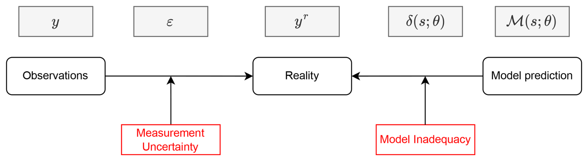
which states that the deviation between the model predictions and the observations results from the superposition of measurement and model errors. As illustrated in Fig. 1, this statistical model establishes the relation between model predictions, observations, and reality. Thus, it is used in the Bayesian calibration framework to find the most probable set of parameters for a given model ℳ and observation y.

Figure 1 Statistical model connecting model predictions, reality, and observations. Adapted from Wu et al. (2018).

However, through this study, we aim to answer a different question: Given a model parameter θ_j, which is the most informative observation $y_j^{*}$ during calibration? Consequently, we isolate the effect of data selection through the use of synthetic data generated from the computational model that guarantees observations to be consistent with the model predictions, hence $\mathit{\delta }(s;\mathit{\theta })=y^r-\mathcal{M}(s;\mathit{\theta })=\mathrm{0}$.

The resulting simplified statistical model can formally be re-written as

$$\begin{array}{}\text{(7)}& \mathit{\theta }={\mathcal{M}}^{-\mathrm{1}}(s;y,\mathit{\epsilon }).\end{array}$$

In reality, of course, the situation is much more involved in the sense that ℳ⁻¹ denotes a computationally hard-to-solve calibration task. The formal write-up, however, indicates the aim of this study, which is not only to estimate parameter θ for a given observational dataset y but also to interpret y as a lever to improve the calibration result. The latter will be referred to as the data selection task. Developing a methodological approach to address this task is the major goal of this study. Although this goal differs from classical Bayesian calibration studies, it turns out that much of the existing work on Bayesian inference can be utilized.

2.2 Bayesian Inference framework

We adopt the Bayesian approach to solve the statistical model formulated in Eq. (7) following Oden (2016). Underpinning everything that follows is Bayes' theorem, which reads

$$\begin{array}{}\text{(8)}& \underset{\text{Posterior}}{\underbrace{P(\mathit{\theta }\mid y)}}={\displaystyle \frac{\underset{\text{Likelihood}}{\underbrace{P(y\mid \mathit{\theta })}}\cdot \underset{\text{Prior}}{\underbrace{P\left(\mathit{\theta }\right)}}}{\underset{\text{Evidence}}{\underbrace{{\int }_{\mathrm{\Theta }}P(y\mid \mathit{\theta })\cdot P\left(\mathit{\theta }\right)\mathrm{d}\mathit{\theta }}}}}\end{array}$$

and captures the relation between prior knowledge of the parameter distribution for θ, observation y, and information return after combining both. Bayes' theorem enables us to determine the optimal parameter values consistent with the observed data by computing the probability distribution of the parameters conditioned on the observations. The resulting distribution is referred to as the posterior distribution – or simply, the posterior – and is denoted by P(θ∣y) in Eq. (8). The posterior represents the updated beliefs about the parameters after observing the data. To arrive at this, we encode our prior beliefs regarding the parameters into a probability distribution known as the prior distribution, also known as the prior, denoted in Eq. (8) as P(θ). We then update the prior distribution by multiplying it with the so-called likelihood function, P(y∣θ), which, as the name implies, represents the likelihood of observing the data y for a given set of parameters θ. The prior distribution typically results from earlier Bayesian calibration steps or requires domain expertise or even empirical knowledge regarding the parameters. The likelihood function, on the other hand, follows from the noise model employed in the statistical model formulation (Eq. 7). Assuming an additive Gaussian noise model with zero mean and covariance Σ, we formulate the likelihood function as shown below, where N_d denotes the dimension of the observation y.

$$\begin{array}{}\text{(9)}& \begin{array}{rl}P(y\mid \mathit{\theta })& ={\displaystyle \frac{\mathrm{1}}{\sqrt{\left(\mathrm{2}\mathit{\pi }{)}^{N_{\mathrm{d}}}\det \right(\mathbf{\Sigma })}}}\\ & \cdot \exp \left({\displaystyle \frac{-\mathrm{1}}{\mathrm{2}}}(y-\mathcal{M}(s;\mathit{\theta }\left){)}^T{\mathbf{\Sigma }}^{-\mathrm{1}}\right(y-\mathcal{M}(s;\mathit{\theta }))\right)\end{array}\end{array}$$

With the prior distribution and the likelihood function defined, we can now compute the posterior distribution using Bayes' theorem presented in Eq. (8). However, computing the posterior distribution involves integrating the product of likelihood and prior with respect to the parameter θ, an integral referred to as the evidence in Eq. (8). This integral is infeasible as soon as the computational model encapsulated in the likelihood function Eq. (9) gets costly to solve. Also, the dimension of the parameter space Θ impacts on computational feasibility. For a high-dimensional parameter distribution, the integral is also high-dimensional, making it one of the primary practical challenges of the Bayesian approach. Following (Gelman et al., 2013; Robert and Casella, 2004), we address this challenge by approximating the posterior distribution using samples generated by Markov Chain Monte Carlo (MCMC) methods, averting the need to calculate the integral. These MCMC samples can be used to approximate the posterior distribution using methods such as kernel density estimation.

A schematic representation of the Bayesian approach is shown in Fig. 2. We begin by defining the prior distributions for the parameters $\mathit{\theta }\in \mathit{\{}{\mathit{\theta }}_{\mathrm{1}},{\mathit{\theta }}_{\mathrm{2}},\mathrm{\dots },{\mathit{\theta }}_m\mathit{\}}$. Then, the likelihood function is used to update these priors, thereby obtaining the posterior distributions. As Fig. 2 illustrates, the likelihood function can be interpreted as the core driver of the process, with data resulting from observations guiding and refining each step. Consequently, the posterior distributions strongly depend on the observations used for calibration. The next section will be devoted to quantifying this dependence, ultimately leading to a better understanding of how to leverage observations y for more informative and reliable posterior distributions.

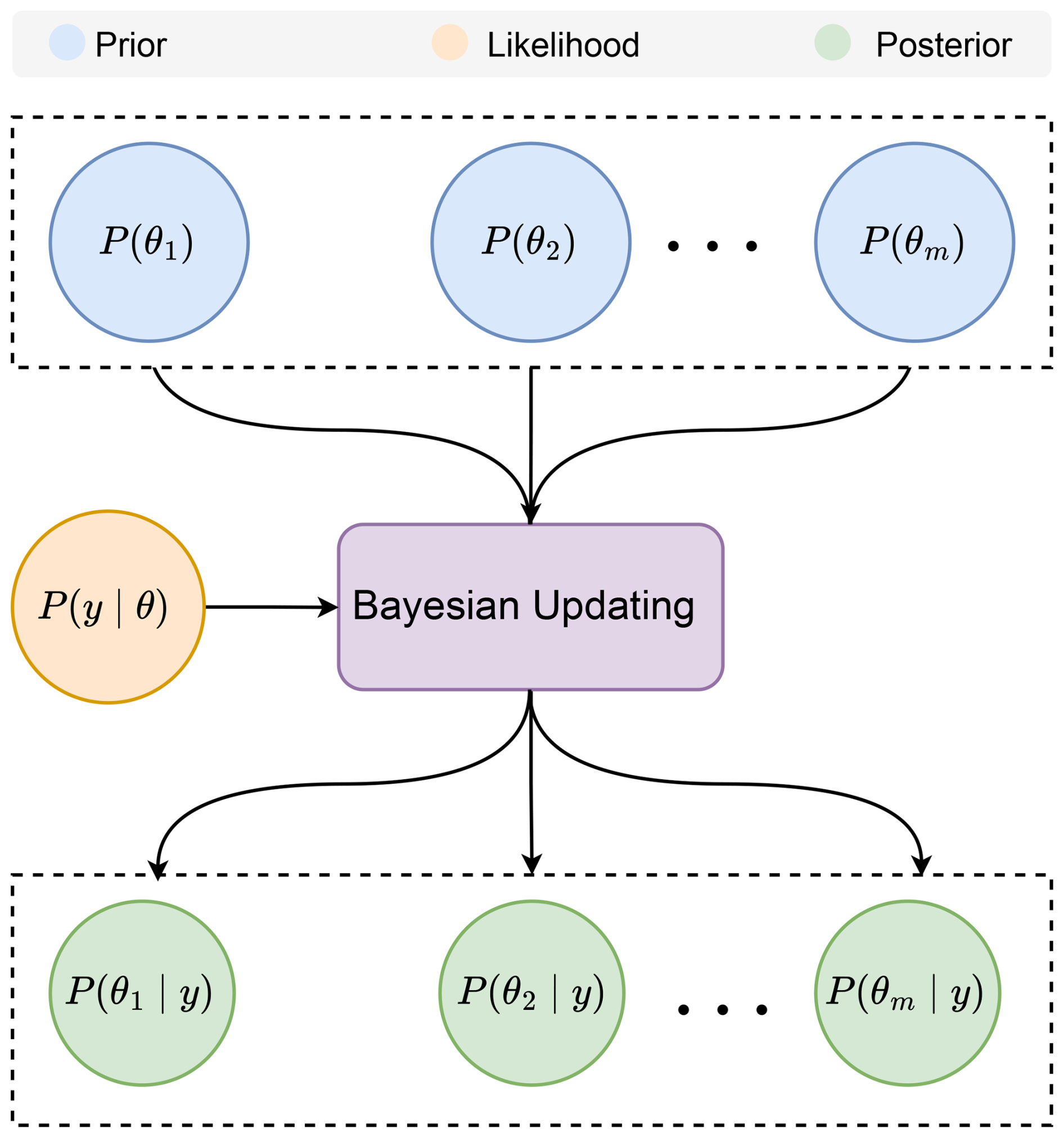
Figure 2 Schematic illustration of the Bayesian inference process. The likelihood function acts as the core driver of updating the prior distribution to posterior distribution based on observational data. The resulting posterior depends strongly on type and quality of the observation.

2.3 Data selection using Information-theoretic measure

In the Bayesian framework, our prior beliefs about the parameters θ are updated by observations, but the extent of this update varies depending on which observations are used. To quantify how informative each candidate observation is, we measure the information gained during calibration with observation y. Observations reduce parameter uncertainty by updating the prior distribution P(θ) to the posterior distribution P(θ∣y). Thus, the information gained during this updating process corresponds to the reduced uncertainty. A fundamental information-theoretic measure of uncertainty is the entropy. For a random variable θ with probability distribution P(θ), entropy H(θ) is given as:

$$\begin{array}{}\text{(10)}& H\left(\mathit{\theta }\right)=-\int P\left(\mathit{\theta }\right)\log P\left(\mathit{\theta }\right)\mathrm{d}\mathit{\theta }\end{array}$$

Higher entropy indicates greater uncertainty about the parameter. Therefore, the change in entropy from prior to posterior quantifies the information gained from an observation. A standard measure to quantify information gain based on change in entropy is KL divergence (Kullback and Leibler, 1951), also known as relative entropy. In the Bayesian setting, KL divergence between the posterior distribution (P(θ∣y)) and the prior distribution (P(θ)), as defined in Eq. (11), admits a direct interpretation as information gain, since it quantifies the reduction in uncertainty about parameter θ achieved by conditioning on observation y. Higher KL divergence indicates greater reduction in uncertainty from prior to posterior, implying that the observation provides greater information about the parameters. Accordingly, we use this quantity as a criterion for data selection, consistent with its standard use in Bayesian optimal experimental design and inverse problems (Haeusel et al., 2026; Chowdhary et al., 2024; Huber et al., 2023; Baptista et al., 2022).

$$\begin{array}{}\text{(11)}& D_{\mathrm{KL}}\left(P\right(\mathit{\theta }\mid y)\Vert P(\mathit{\theta }\left)\right)=\int P(\mathit{\theta }\mid y)\log \left({\displaystyle \frac{P(\mathit{\theta }\mid y)}{P\left(\mathit{\theta }\right)}}\right)\mathrm{d}\mathit{\theta }\end{array}$$

In the context of our work, we focus on calibrating landslide runout models with conceptual parameters that cannot be measured physically. For these parameters, we have limited prior information such as physically plausible bounds derived from literature and domain expertise. We therefore use uniform priors within these bounds, following standard practice in landslide runout calibration (Moretti et al., 2020; Aaron et al., 2019; Navarro et al., 2018). For uniform priors, the prior entropy H(P(θ)) is constant, so maximizing KL divergence is equivalent to minimizing the posterior entropy H(P(θ|y)) (see Appendix A for derivation). In our numerical experiments with uniform priors, maximizing KL divergence is therefore equivalent to selecting observations that minimize posterior entropy, yielding the sharpest and most informative posterior distributions.

A schematic representation of the data selection process is shown in Fig. 3. We use the Bayesian calibration approach detailed in Sect. 2.2 to calibrate the parameters θ using multiple observational datasets, where $y_i\in \mathit{\{}{y}_{\mathrm{1}},y_{\mathrm{2}},\mathrm{\dots },y_n\mathit{\}}$ denotes the ith dataset. Note that each individual dataset y_i can either constitute a single scalar observation or a sequence of observations such as time series of velocity or position. Consequently, we obtain n posterior distributions, one for each observational dataset, which we compare against the prior distribution using the KL divergence defined in Eq. (11). This yields a quantitative measure of the information that each observation contributes to the calibration process, allowing us to identify the most informative dataset ${\stackrel{\mathrm{‾}}{y}}^{*}$ to infer the parameters θ. The bar above ${\stackrel{\mathrm{‾}}{y}}^{*}$ indicates its aggregate nature. Although ${\stackrel{\mathrm{‾}}{y}}^{*}$ maximizes the information for joint calibration, it may not be the most informative dataset to calibrate a specific parameter θ_j.

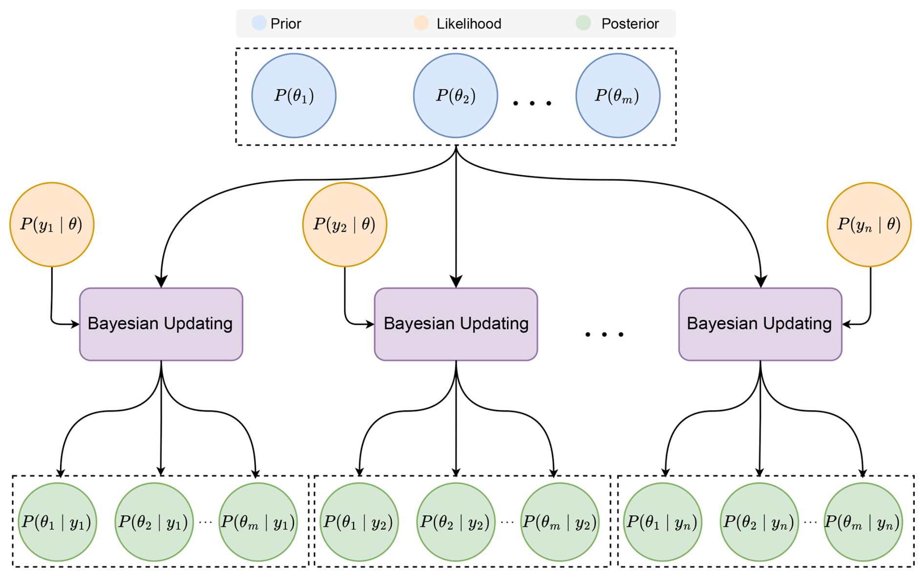
Figure 3 Schematic illustration of the Bayesian data selection process using information-theoretic metrics. Multiple calibration routines are performed in parallel, each using the same likelihood function but leveraging different observations to update the prior distributions. By comparing each resulting posterior distribution against the prior, we can quantify the information gained during calibration relative to observations.

To identify the most informative dataset for a given parameter θ_j, we marginalize the posteriors with respect to parameters and obtain n posteriors for each parameter ${\mathit{\theta }}_j\in \mathit{\{}{\mathit{\theta }}_{\mathrm{1}},{\mathit{\theta }}_{\mathrm{2}},\mathrm{\dots },{\mathit{\theta }}_m\mathit{\}}$, given as $\mathit{\left\{}P\right({\mathit{\theta }}_j\mid y_{\mathrm{1}}),P({\mathit{\theta }}_j\mid y_{\mathrm{2}}),\mathrm{\dots },P({\mathit{\theta }}_j\mid y_n\left)\mathit{\right\}}$. We then compute the KL divergence between the individual prior distribution P(θ_j) and the posterior distributions of θ_j corresponding to each of the observations. The generalized formulation for computing the KL divergence between the prior and posterior distribution of the parameter θ_j calibrated using observation y_i is given in Eq. (12).

$$\begin{array}{}\text{(12)}& \begin{array}{rl}& D_{\mathrm{KL}}^{i,j}\left(P\right({\mathit{\theta }}_j\mid y_i)\Vert P({\mathit{\theta }}_j\left)\right)=\\ & \int P({\mathit{\theta }}_j\mid y_i)\log \left({\displaystyle \frac{P({\mathit{\theta }}_j\mid y_i)}{P\left({\mathit{\theta }}_j\right)}}\right)\mathrm{d}{\mathit{\theta }}_j\end{array}\end{array}$$

Thus, for each parameter θ_j, we have n KL divergence values denoted as $D_{\mathrm{KL}}^{i,j}$. These values correspond to observations y_i, with i ranging from {1…n}. Since these values quantify the information gained through the Bayesian update, we can utilize them to select the dataset $y_j^{*}$ that constitutes the most informative dataset for calibrating the parameter θ_j.

$$\begin{array}{}\text{(13)}& \begin{array}{rl}& \text{Data selection task:}\\ & \text{For a given parameter }{\mathit{\theta }}_j\text{find}{y}_j^{*}=\arg \underset{i\in \mathit{\{}\mathrm{1},\mathrm{\dots },n\mathit{\}}}{max}{D}_{\mathrm{KL}}^{i,j}\end{array}\end{array}$$

Bayesian calibration combined with data selection based on KL divergence constitutes the methodology of Bayesian data selection. This allows us to understand and quantify how adept available observations are in constraining a given parameter.

2.4 Workflow

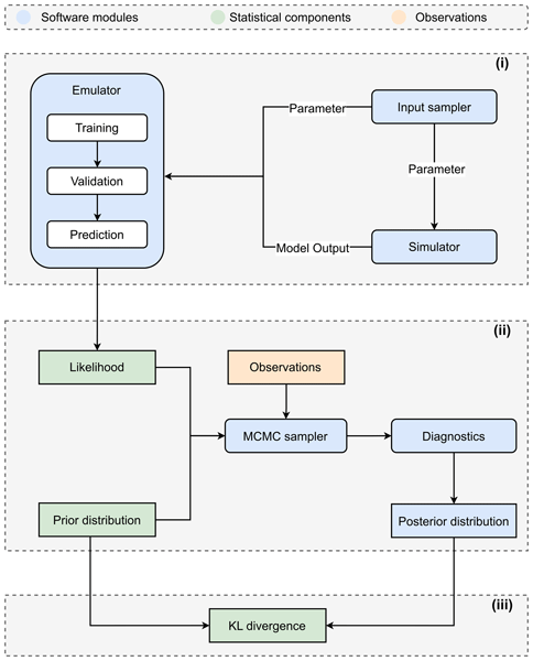
We implement our Bayesian data selection workflow, as illustrated in Fig. 4, using PSimPy, a Python-based package for predictive and probabilistic simulations (Zhao, 2022). The workflow comprises three distinct phases: (i) Surrogate Modeling; (ii) Bayesian Parameter Calibration; (iii) Data Selection.

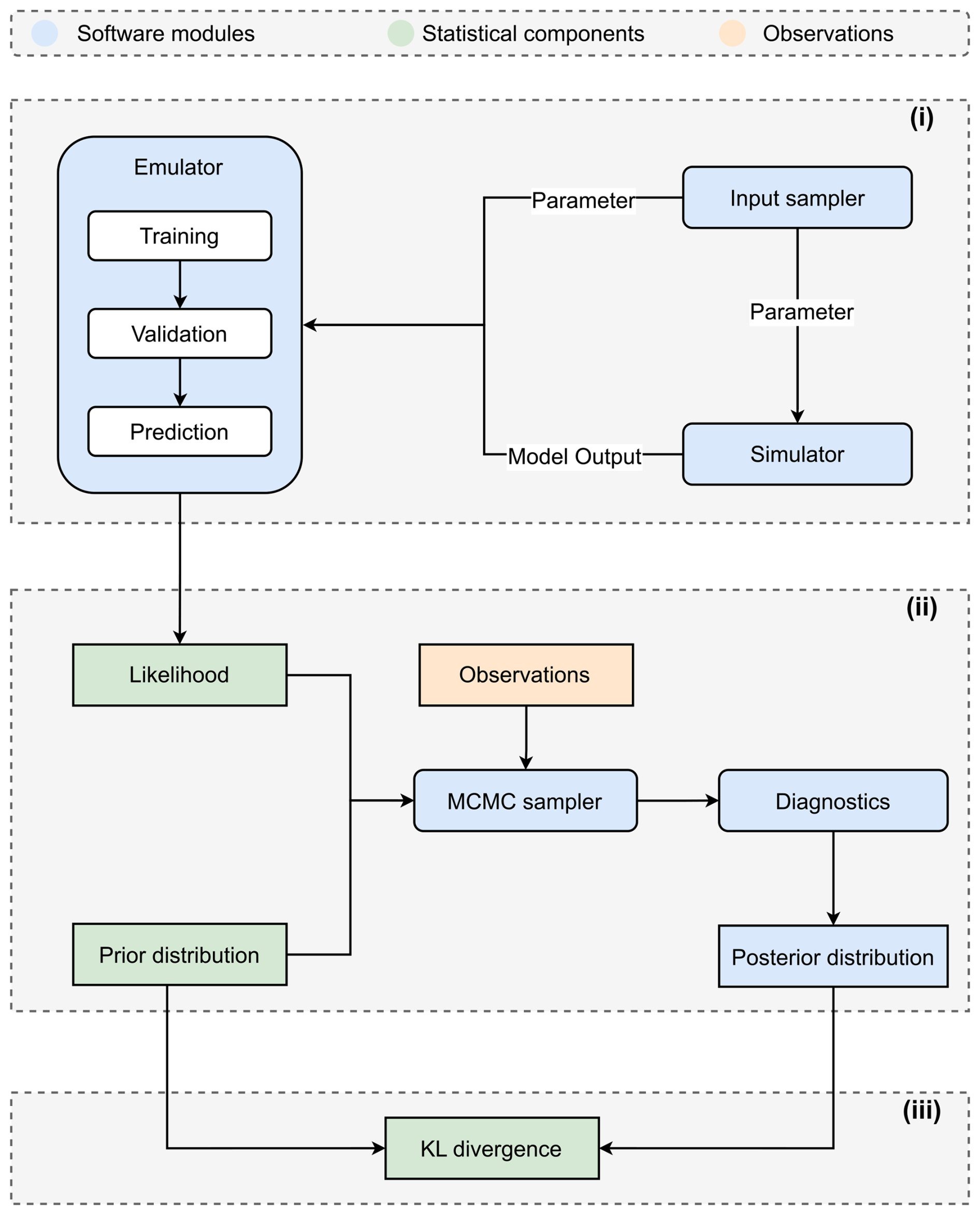
Figure 4 Overview of the Bayesian data selection workflow. The workflow consists of three key phases: (i) Surrogate Modeling, where a computationally efficient surrogate replaces the expensive forward model; (ii) Bayesian Parameter Calibration, where an MCMC sampler is used to infer the posterior distribution of the parameters; and (iii) Data Selection, where KL divergence quantifies the information gain from different observational data.

2.4.1 Surrogate Modeling

Surrogate modeling serves as a computational enabler to overcome computational bottlenecks in calculating the KL divergence. As illustrated in Eq. (11), calculating KL divergence requires posterior distributions, which are approximated through MCMC sampling (see Sect. 2.2). The accuracy of this approximation is based on the ability of MCMC chains to effectively explore the posterior space, which typically requires a large number of samples. Each sample necessitates evaluating the likelihood function, entailing one complete execution of the computational model. Therefore, this approach becomes infeasible for computationally expensive models. To tackle this challenge, we employ GP emulators, a non-intrusive surrogate modelling technique that reduces computational costs in Bayesian calibration workflows (Zhao and Kowalski, 2022). The widespread adoption of GP emulators stems from their ability to provide probabilistic predictions, allowing for rigorous quantification of the uncertainty associated with predictions. Furthermore, they offer efficient performance with limited training datasets compared to other machine learning approaches. Mathematically, a GP is defined by a mean function m(x) and a covariance function $k(x,x^{\prime })$ as shown in Eq. (14).

$$\begin{array}{}\text{(14)}& f\left(x\right)\sim \mathcal{G}\mathcal{P}\left(m\right(x),k(x,x^{\prime }\left)\right)\end{array}$$

Both the mean and covariance functions in Eq. (14) are parameterized by hyperparameters that are inferred from the training data. To implement the GP emulator, we utilize the emulator module of PSimPy, which harnesses RobustGaSP, an R package for Gaussian stochastic process emulation that provides robust estimates of the hyperparameters leading to enhanced predictive performance (Gu and Berger, 2016).

Figure 4 illustrates the key steps involved in the surrogate modeling phase. We start by generating a set of input parameters using the sampler module of PSimPy, which leverages space-filling schemes like Latin hypercube sampling. Next, we employ the simulator module to evaluate our computational model (ℳ), at these input points. The resulting model outputs are then post-processed according to the emulation strategy determined by the observation dimensionality. For scalar observations, we emulate the parameter-to-observable map, replacing the forward model ℳ in Eq. (9) with a cost-effective surrogate $\widehat{\mathcal{M}}$. Alternatively, for high-dimensional observations (e.g., velocity or position time series), we directly emulate the likelihood function, which quantifies the mismatch between model output and observation. This approach leverages the fact that the likelihood is scalar-valued regardless of observation dimensionality, thereby avoiding the computational challenges of constructing GP emulators with high-dimensional outputs. These post-processed outputs, together with the set of input points, constitute our training data used to build and train the GP emulator. We then validate the trained surrogate using k-fold cross-validation. After successful validation, the surrogate model is available for predictions.

2.4.2 Bayesian Parameter calibration

The trained GP surrogate from the surrogate modeling phase replaces the expensive computational model in the likelihood function in Eq. (9), allowing us to sample the posterior distribution using MCMC methods. For this purpose, we utilize the mcmc sampler of PSimPy, which is based on Python's emcee package, an affine invariant MCMC ensemble sampler (Foreman-Mackey et al., 2013). This implies that the sampler is unaffected by affine transformations of parameter space, allowing it to sample complex probability distributions without the need for problem-specific tuning. Furthermore, it employs multiple chains that evolve in parallel, resulting in an efficient exploration of the probability distribution. Additionally, we assess the convergence of the MCMC chains using the diagnostics module, leveraging Python's Arviz package (Kumar et al., 2019). Using this module, we qualitatively assess the convergence using trace plots and then quantify it using standard diagnostic metrics such as Gelman-Rubin statistic $\widehat{R}$ (see Appendix B).

2.4.3 Data selection

In this phase, we compute the KL divergence between the posterior and prior distributions obtained from the Bayesian calibration phase. As discussed in Sect. 2.3, this involves computing the intractable integral, which we approximate using the distance-based KL divergence estimator proposed by Wang et al. (2009). To this end, we incorporate the code from Hartland (2020) into our workflow, as it implements the estimators described by Wang et al. (2009). We marginalize the posterior distributions from the Bayesian calibration phase with respect to the parameters and compute KL divergence, as presented in Sect. 2.3. By calibrating m parameters using n observations, we end up with n×m KL divergence matrix, as shown in Fig. 5, where each entry, $D_{\mathrm{KL}}^{i,j}$, quantifies the information that ith observation y_i provides for calibrating jth parameter θ_j. Using this KL divergence matrix we can identify the most informative observation $y_j^{*}$ for a given parameter θ_j by maximizing the KL divergence across available observations (as defined in Eq. 13).

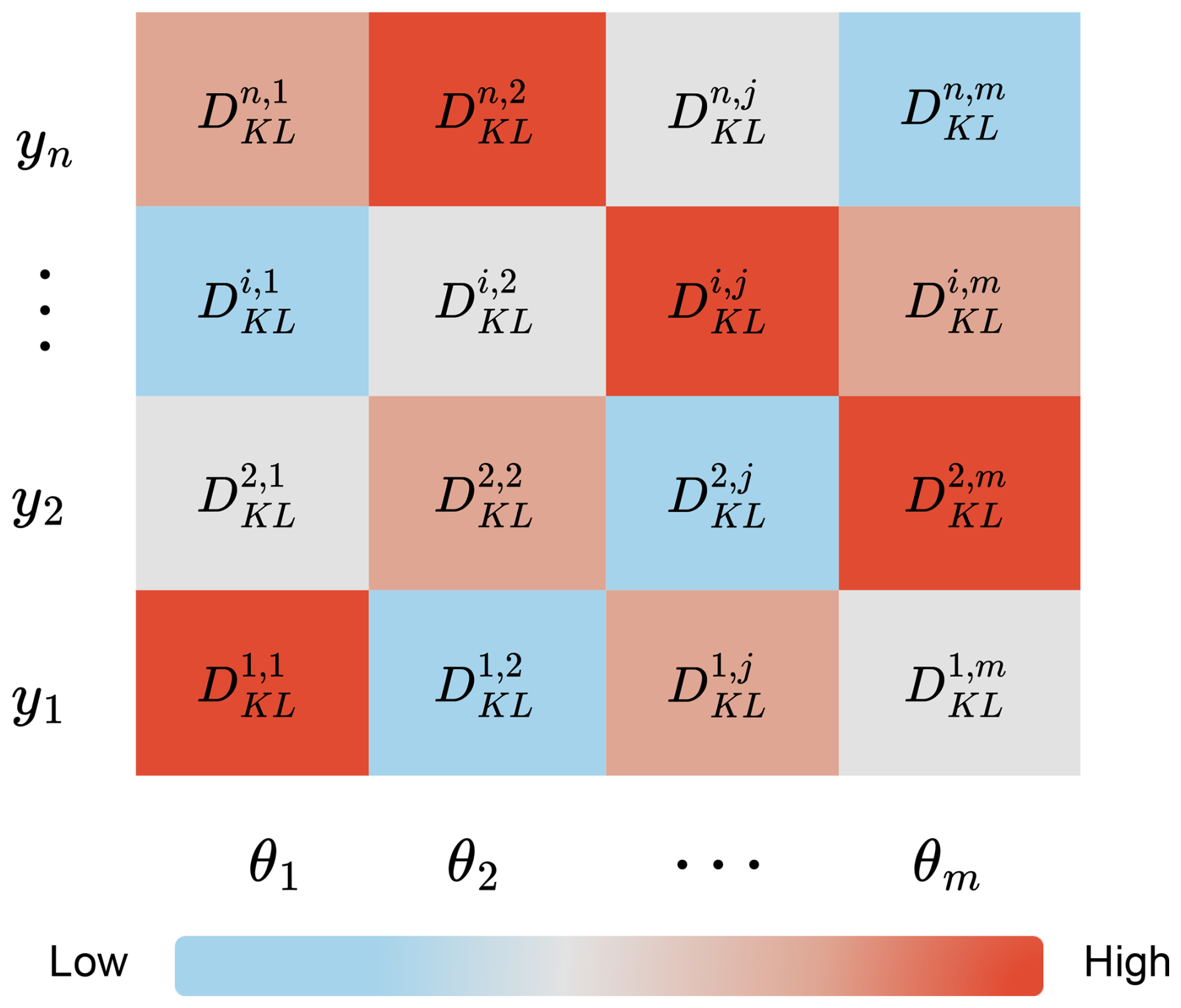
Figure 5 KL divergence matrix generated in the calibration of m parameters with n observation. Each entry of the matrix quantifies the information provided by observation y_i for calibrating parameter θ_j.

3 Case Study

This study investigates how the choice of observational data influences the calibration of model parameters. Specifically, we aim to identify the most informative dataset for calibrating a given parameter. To this end, we performed multiple calibration routines using the Bayesian calibration workflow outlined in Sect. 2.4, each with a different observational dataset. We then compute the KL divergence between the prior and posterior distributions to quantify the information gained from each dataset. As shown in Sect. 2.1, this process requires three key components: (1) a computational model with parameters to be calibrated, (2) observations to update those parameters, and (3) a noise model that captures uncertainty in observations. The noise model has already been described in Eq. (4). This section describes the computational model and multiple observational datasets used in the calibration.

3.1 Computational Model

Hungr (1995) categorized the numerical landslide runout models into models based on continuum mechanics and lumped mass models. In both models, gravity primarily drives the motion, while a friction term, dependent on the chosen rheological model, resists it. However, due to the complexity of landslide dynamics, these rheological formulations often involve conceptual parameters that are not directly measurable and must, therefore, be inferred through model calibration. While lumped mass models idealize the sliding landslide mass as a single mass point, continuum-based models treat it as a spatially distributed deformable mass governed by conservation laws (Yildiz et al., 2023). As a result, lumped mass models are limited in their ability to represent internal deformations, which are captured by continuum-based models, thereby enabling a more accurate simulation of flow dynamics and deposit morphology (Hergarten, 2024). However, lumped mass models offer a conceptually straightforward framework for estimating bulk characteristics such as runout distances, velocities, and accelerations (Zahra, 2010). Furthermore, conceptual simplicity allows for a clear, tractable mapping between model parameters and landslide dynamics, which is often obscured in continuum models. Thus, we deliberately employ lumped mass models, given that the primary aim of this study is to assess how observational data influence parameter calibration.

Governing equation of a lumped mass model is mathematically described using Newton's second law of motion, as shown in Eq. (15).

$$\begin{array}{}\text{(15)}& {\displaystyle \frac{\mathrm{d}u}{\mathrm{d}t}}=g\sin \mathit{\beta }-{\displaystyle \frac{F_{\mathrm{res}}}{m}}\end{array}$$

Here, u is the tangential velocity of the idealized mass point, g is the gravitational constant, β is the slope angle, and F_res is the resisting force term. We choose the Voellmy rheological model, which includes a classical dry Coulomb friction coefficient μ representing the basal resistance to landslide motion, along with a velocity-dependent friction term known as the turbulent friction coefficient ξ. The corresponding formulation of the resistance force is given as:

$$\begin{array}{}\text{(16)}& F_{\mathrm{res}}=\mathit{\mu }mg\cos \mathit{\beta }+{\displaystyle \frac{mg}{\mathit{\xi }}}{u}^{\mathrm{2}}\end{array}$$

In addition to the rheological parameters described in Eq. (16) ({μ,ξ}), we need to provide parameterized information $(s\in \mathit{\{}T(x,y),u_{x_{\mathrm{0}}},u_{y_{\mathrm{0}}},x_{\mathrm{0}},y_{\mathrm{0}}\mathit{\left\}}\right)$ specifying the landslide simulation scenario, where T(x,y) denotes the topography and the other parameters represent the initial conditions, such as initial velocity and position. In this study, we employ a synthetic topography representing an idealized digital elevation model (DEM). As shown in Fig. 6, the topography consists of a curved longitudinal profile that is uniform in the transverse direction.

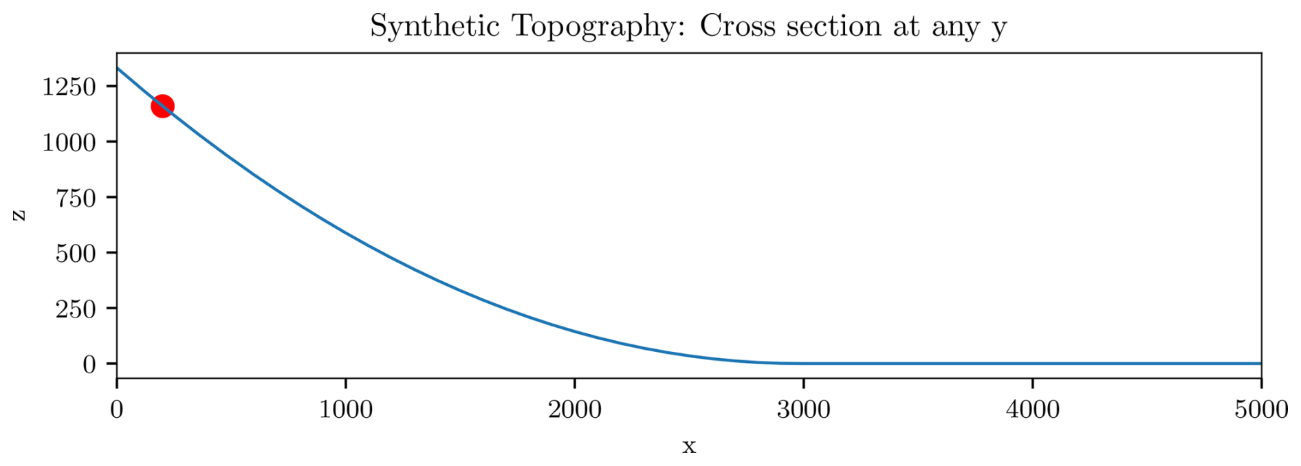
Figure 6 Vertical cross-section of the synthetic topographic model used in this study, with elevation (z) plotted against the horizontal coordinate (x). The topography is constant along the transverse direction. The red marker denotes the position of the initial release point projected onto this cross-section.

3.2 Observational datasets

We curate a diverse set of observations, each capturing different aspects of landslide dynamics, to systematically assess the influence of data selection on Bayesian calibration outcome. However, obtaining such diverse observational datasets in the real world is often infeasible due to logistical and financial constraints (Seibert et al., 2024). To address this, the study uses synthetic data to calibrate the friction parameters of the lumped mass model described in Sect. 3.1. Synthetic data also provide the advantage of known ground-truth parameters that can be directly compared with the inferred values.

The observational data used in this study can be categorized as: (1) aggregate observations, which reflect bulk characteristics such as runout distance and maximum velocity, and (2) time series observations, which capture the velocity and position of the sliding mass over time. We generate these observations by evaluating the lumped mass model with a selected set of friction parameters. These parameters are arbitrarily selected within the bounds reported in the literature: the dry Coulomb friction coefficient μ=0.23, chosen from the range [0.02,0.3], and the turbulent friction coefficient ξ=1000, chosen from the range [100,2200]. The lumped mass model is then evaluated with these parameters, generating a time history of velocity and position of the sliding mass. These outputs are post-processed to create both aggregate and time series observational datasets, with added noise to mimic real-world measurement uncertainty. For aggregate observations, which are scalar quantities (e.g., runout distance or maximum velocity), perturbations are drawn from a Gaussian distribution with zero mean and a standard deviation equal to one-tenth of the scalar's magnitude. For time series observations, we assume that errors in time steps are independent of each other. Then, each time step is perturbed using noise drawn from a Gaussian distribution with zero mean and unit standard deviation and then scaled by one-tenth of the maximum value in the respective time series (velocity or position). The resulting noisy values are clipped to zero wherever they become negative.

3.3 Design of Numerical Experiments

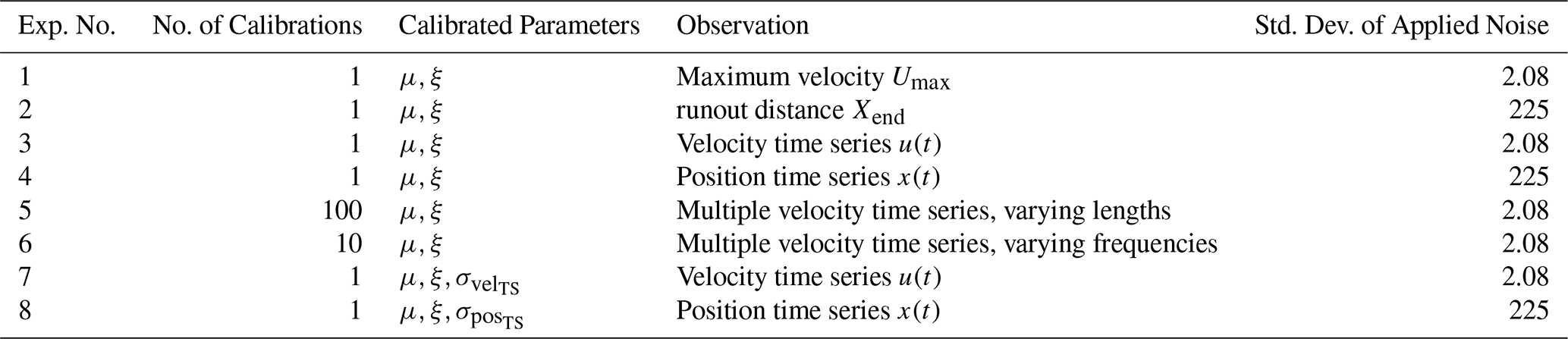
We conducted a series of eight numerical experiments using the synthetic datasets described in Sect. 3.2 to calibrate the friction parameters of the lumped mass model. In experiments 1 through 4, we vary the information content and granularity of the observational data to examine the influence of data selection on the calibration outcome. Experiments 1 and 2 use aggregated observations – maximum velocity and runout distance, respectively – while Experiments 3 and 4 use time series data of velocity u(t) and position x(t).

Experiments 5 and 6 investigate how the temporal characteristics of time series data, specifically length, and resolution, impact calibration outcomes. While experiment 5 involves calibration routines performed using time series data of varying lengths, experiment 6 uses time series data of varying resolution. Together, these experiments evaluate how the length and resolution of the time series data influence the accuracy of parameter estimation.

Experiments 7 and 8, extend the calibration to include the noise model’s discrepancy parameter (see Eq. 4), which was previously fixed using heuristic assumptions. These experiments explore how jointly estimating observational uncertainty, along with μ and ξ, affects calibration outcomes. Velocity and position time series are again used as observational datasets in these cases. In all the 8 experiments we assume uniform priors for the friction parameters. The bounds for the priors are chosen from the literature as discussed in Sect. 2.3, for $\mathit{\mu }\in [\mathrm{0.02},\mathrm{0.3}]$ and $\mathit{\xi }\in [\mathrm{100},\mathrm{2200}]$ m s⁻². Additionally in experiment 7 and 8, we assume an uniform prior for the discrepancy parameters ${\mathit{\sigma }}_{{\mathrm{vel}}_{\mathrm{TS}}}$ and ${\mathit{\sigma }}_{{\mathrm{pos}}_{\mathrm{TS}}}$ with bounds [1,5] and [0,500] respectively.

Table 1 Summary of numerical experiments investigating the impact of observational data choice on Bayesian calibration outcomes. Experiments 1–6 calibrate friction coefficients (μ, ξ) using different observation types, while experiments 7–8 additionally calibrate discrepancy parameters (${\mathit{\sigma }}_{{\mathrm{vel}}_{\mathrm{TS}}}$, ${\mathit{\sigma }}_{{\mathrm{pos}}_{\mathrm{TS}}}$). Apart from experiments 5–6, all other experiments involve single calibration routines. All experiments use synthetic observations generated by adding random noise drawn from a Gaussian distribution with zero mean and specified standard deviations.

4 Results

This section includes results for the curated set of numerical experiments discussed in Sect. 3.3. We adopt the workflow presented in Sect. 2.4 and the associated data: (i) Training dataset including set of sampled parameters and the corresponding model outputs; (ii) Ground-truth data used to generate the synthetic observations detailed in Sect. 3.2 are archived in this repository https://doi.org/10.5281/zenodo.17120721 (Kumar, 2025).

4.1 Experiment 1: Calibration with maximum velocity as observation

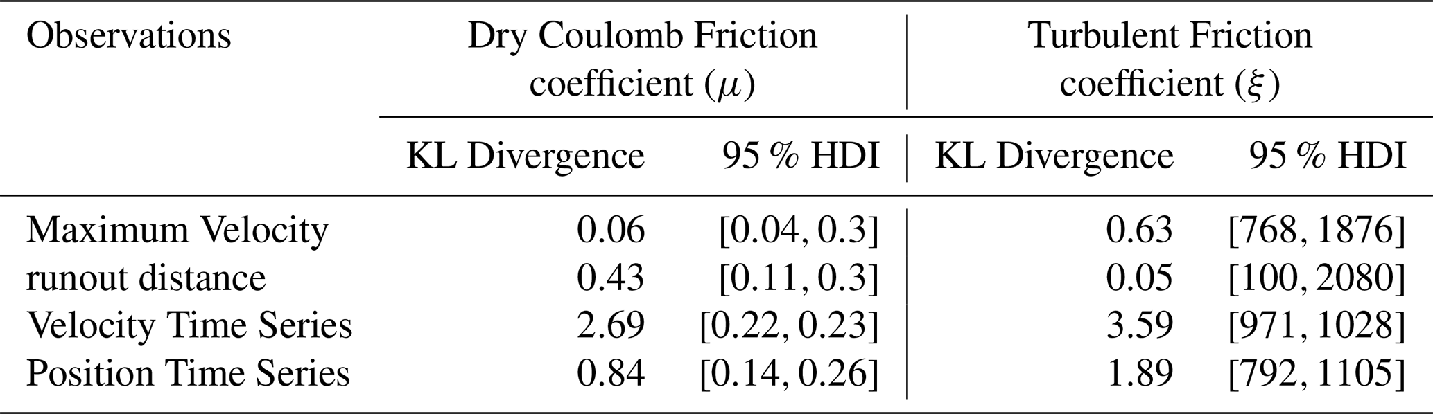
Figure 7 illustrates the prior distribution of the friction parameters and their corresponding posterior distributions obtained by performing the calibration using the maximum velocity (U_max) as observation. The maximum a posteriori (MAP) estimates, indicated by the black dashed lines in Fig. 7a and b, provide the most probable values for the parameters. The MAP estimate for μ is 0.284, while for ξ it is 1187. The uncertainty associated with these estimates is summarized by highest density intervals (HDI), listed in the Table 2. The parameter values within 95 % HDI have a higher probability than those outside this interval. Thus, a narrower HDI, as observed for ξ, indicates a lower degree of uncertainty. This suggests that the maximum velocity provided greater information for ξ during calibration. This is also highlighted by the difference in KL divergence values (refer Table 2), which had a higher value for ξ.

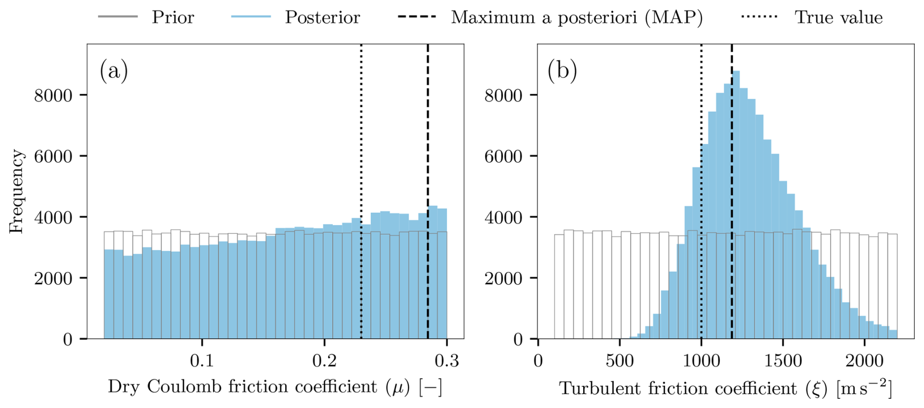
Figure 7 Posterior and prior distributions of (a) Dry Coulomb friction coefficient (μ) and (b) Turbulent friction coefficient (ξ) based on calibration with maximum velocity (U_max) as observation. Maximum velocity conveyed more information about ξ during calibration, as reflected in the narrower posterior distribution.

Table 2 Kullback-Leibler Divergence and 95 % Highest Density Intervals for friction coefficients calibrated using multiple datasets.

4.2 Experiment 2: Calibration with runout distance as observation

We repeated the calibration of the friction parameters using the runout distance as observation, and the results are depicted in Fig. 8. This calibration yielded a MAP estimate for μ of 0.277, nearly identical to the MAP value presented in Fig. 7a. However, the 95 % HDI listed in Table 2, is considerably shorter, suggesting greater confidence in the estimate. In contrast, the 95 % HDI interval for ξ has widened, and even the MAP estimate (shown in Fig. 8b) of 159 significantly differs from the true value of 1000. This indicates that more information was gained for μ when calibrated with the runout distance. A higher KL divergence value of 0.43 for μ compared to 0.05 for ξ further corroborates this assertion, refer Table 2.

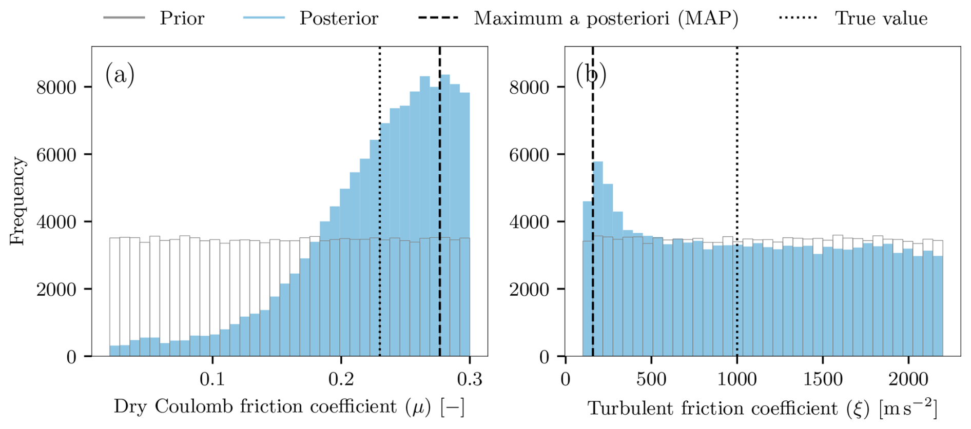
Figure 8 Posterior and prior distributions of (a) Dry Coulomb friction coefficient (μ) and (b) Turbulent friction coefficient (ξ) based on a calibration with runout distance (X_end) as observation. Greater contraction of the posterior of μ indicates higher information gain during calibration with the runout distance.

4.3 Experiment 3: Calibration with velocity time series as observation

A third calibration was conducted using the velocity time series u(t), and the parameter distributions are presented in Fig. 9. Unlike the results of calibration with aggregated data (e.g., maximum velocity and runout distance), we see a significant information gain for both μ and ξ, reflected by the much smaller 95 % HDI listed in Table 2. Even the KL divergence values outlined in Table 2 are significantly higher than those corresponding to the aggregated data. Furthermore, the MAP estimates for both parameters are nearly identical to the true values.

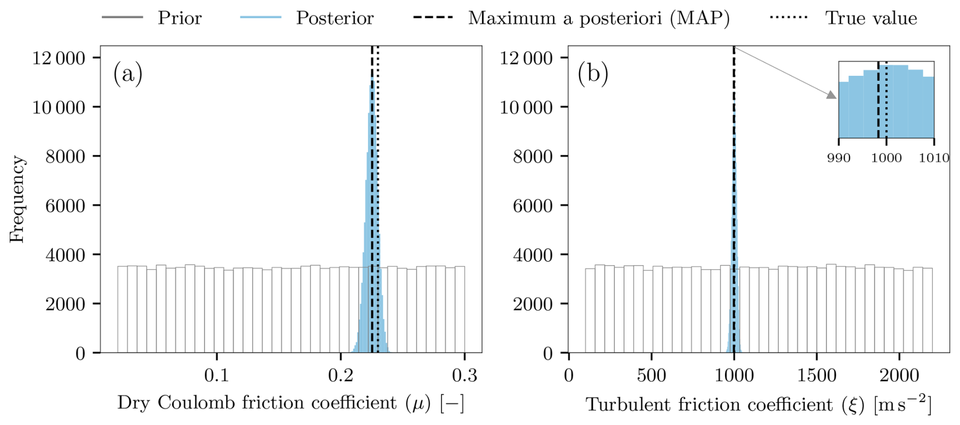
Figure 9 Posterior and prior distributions of (a) Dry Coulomb friction coefficient (μ) and (b) Turbulent friction coefficient (ξ) based on a calibration with velocity time series as observation. Velocity time series provides considerably greater information about both μ and ξ during calibration, as evidenced by the narrower posterior distributions.

4.4 Experiment 4: Calibration with position time series as observation

Figure 10 shows the parameter distributions, calibrated with position time series, x(t). Again, we observed information gain for both parameters, reflected in the contracted posterior distributions, illustrated in Fig. 10a and b. MAP estimates for μ and ξ are also closer to the true values compared to the estimates in Figs. 7 and 8. However, this information gain is lower than that observed in the calibration using velocity time series (u(t)), as indicated by the lower KL divergence values of 0.84 for μ and 1.89 for ξ, compared to 2.69 and 3.59 (as shown in Table 2).

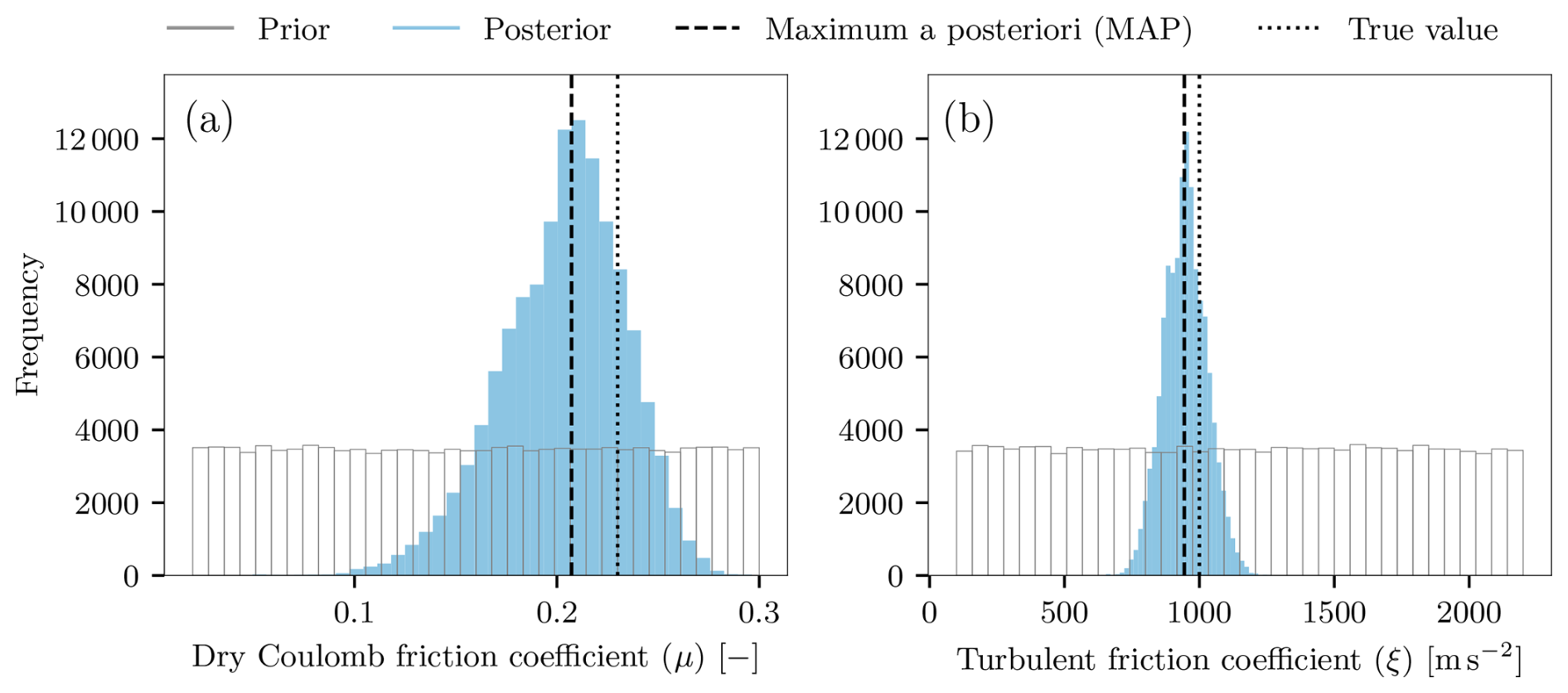
Figure 10 Posterior and prior distributions of (a) Dry Coulomb friction coefficient (μ) and (b) Turbulent friction coefficient (ξ) based on calibration with position time series as observation. Similar to velocity time series, position time series also provides information about both parameters, albeit to a lesser extent.

4.5 Experiment 5: Value of information in data: Length of velocity time series data

We calibrated the friction parameters with 100 different datasets of velocity time series, each containing a varying number of time steps. Seven selected posterior distribution of ξ from these calibrations is depicted in Fig. 11, with the y-axis listing the number of velocity time steps used in the calibration. Calibrating with a higher number of time steps led to greater information gain, reflected in the contracting posteriors with increasing time step count. However, from the Fig. 11, we can see that the difference between the posteriors in the initial time steps is considerably greater than the posteriors in the later time steps. This suggests that the rate of information gain decreases as we use more time steps for calibration.

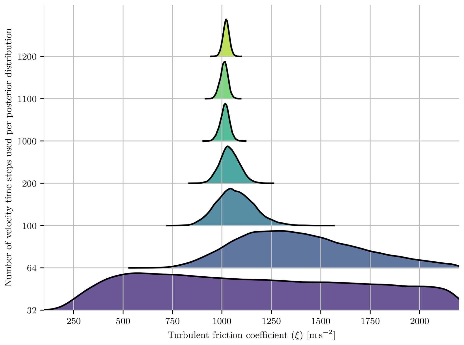
Figure 11 Posterior distributions of turbulent friction coefficient ξ calibrated with a varying number of velocity time steps. The rate of information gain is more profound in the initial time steps than the later.

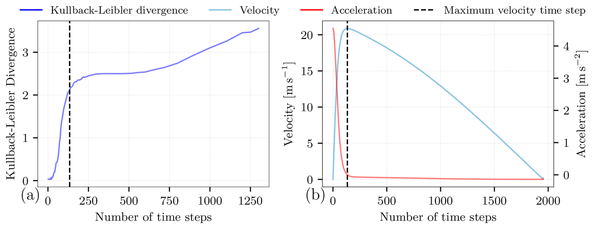
Figure 12 (a) Variation of Kullback-Leibler divergence of the posterior and prior distributions of turbulent friction coefficient ξ with velocity time steps. (b) Variation of velocity and acceleration with time steps.

Figure 12a, plots the variation of the KL divergence of the posterior and prior distributions of ξ with the number of velocity time steps used for calibration. Increasing number of time steps resulted in higher KL divergence, indicating a positive correlation between the information gain and the number of time steps. However, the initial steep slope of the plot in Fig. 12a and its subsequent plateauing point to a diminishing return effect, where additional time steps beyond a critical threshold yield progressively smaller information gain. Interestingly, this threshold corresponds to the time step at which velocity attains its peak, as seen in Fig. 12b.

4.6 Experiment 6: Value of information in data: Temporal resolution of velocity time series data

Figure 13 illustrates the posterior distributions of ξ calibrated using velocity time series datasets of varying temporal resolutions. Each posterior distribution is associated with a specific time step size indicated on the y-axis. For example, a time step size of 4 on the y-axis indicates that the corresponding posterior was generated using a velocity time series of time step size 4. As the resolution of the time series data increases (i.e., with a smaller time step size), the information gain increases, as evidenced by the contracting posteriors.

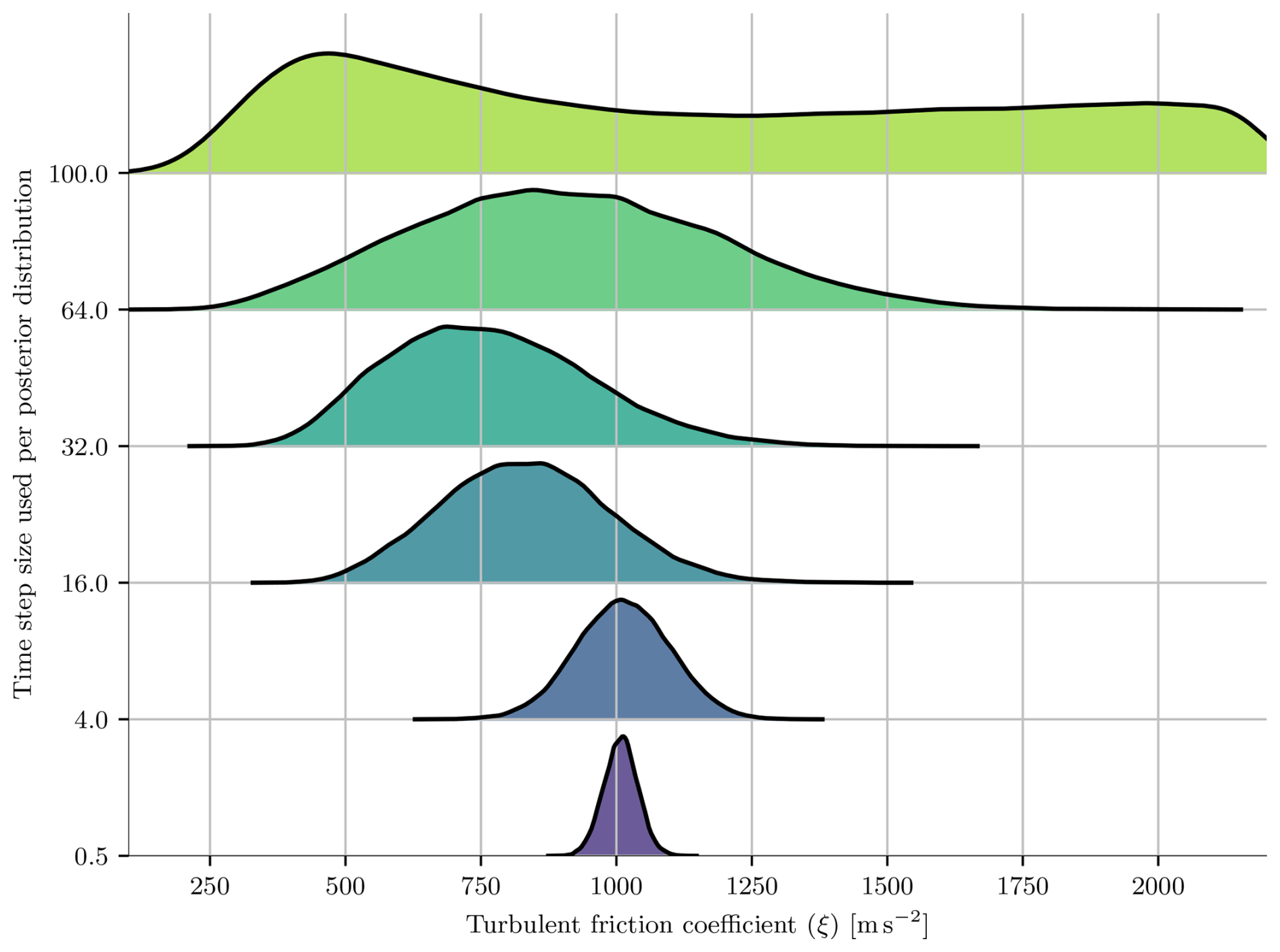
Figure 13 Posterior distributions of turbulent friction coefficient ξ calibrated with a varying temporal resolution of the velocity data. The information gained during calibration increases with temporal resolution.

4.7 Experiment 7 and 8: Calibration of the discrepancy parameters

Figures 7, 8, 9, and 10, presented posterior distributions of friction parameters calibrated using multiple datasets listed in Table 2. During these calibrations, we made heuristic assumptions for the discrepancy parameter σ of the noise model, refer to Sect. 2.1 for detailed discussion. However, we can include this parameter in the calibration routine and calibrate it along with the friction parameters. Figure 14, depicts the prior and posterior distributions of discrepancy parameters corresponding to velocity and position time series. In Fig. 14a, we see that using velocity time series u(t), we can learn extensively for the velocity discrepancy parameter ${\mathit{\sigma }}_{{\mathrm{vel}}_{\mathrm{TS}}}$, indicated by the highly contracted posterior. Similarly, the position time series provides substantial information regarding the position discrepancy parameter ${\mathit{\sigma }}_{{\mathrm{pos}}_{\mathrm{TS}}}$, refer Fig. 14b.

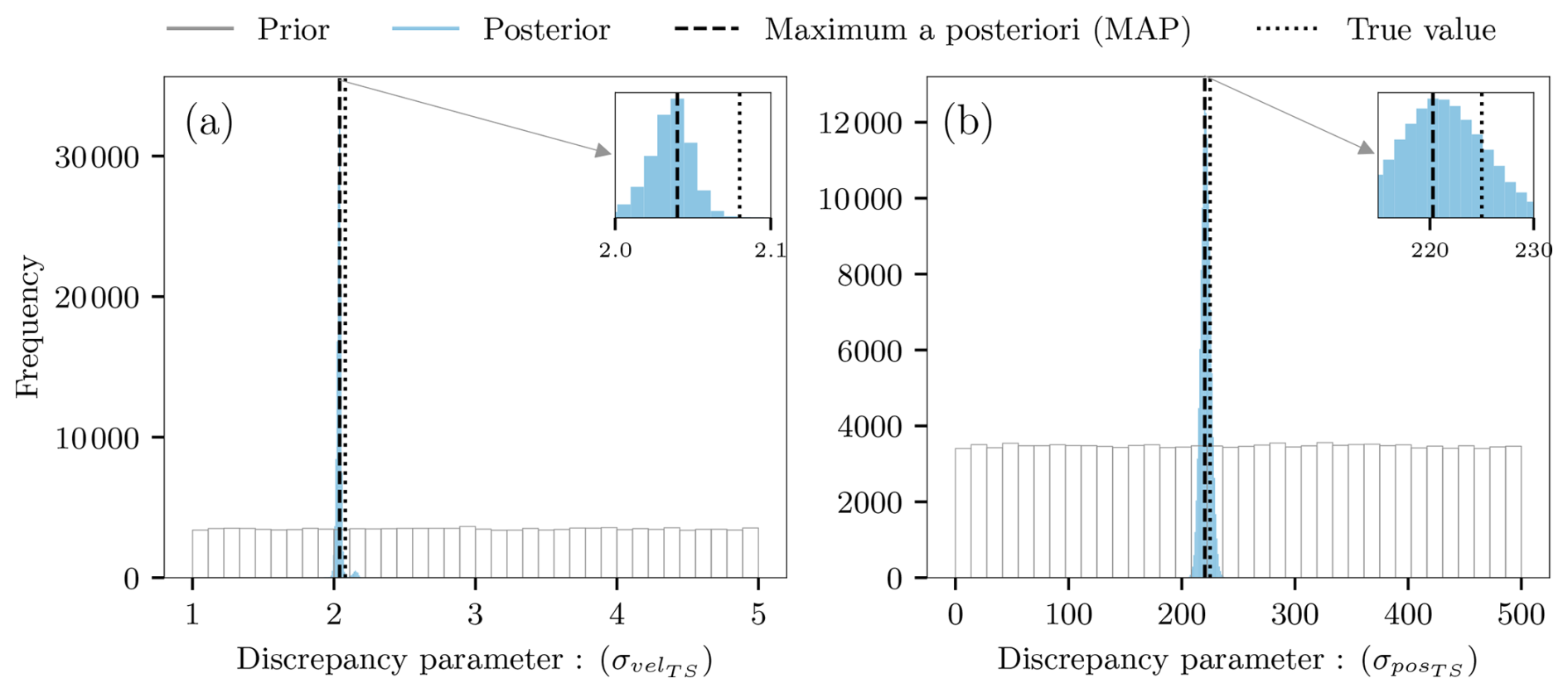
Figure 14 Posterior and prior distributions of (a) Velocity discrepancy parameter (${\mathit{\sigma }}_{{\mathrm{vel}}_{\mathrm{TS}}}$) and (b) Position discrepancy parameter (${\mathit{\sigma }}_{{\mathrm{pos}}_{\mathrm{TS}}}$) based on a calibration with velocity and position time series respectively.

5 Discussions

In our numerical experiments, we investigated the impact of the scope and quantity of the data used as observations in the Bayesian parameter calibration of landslide runout models. To this end, we calibrated the friction parameters of a lumped mass model, namely the dry Coulomb friction coefficient (μ) and the turbulent friction coefficient (ξ), with a diverse set of observational data summarized in Table 1. Using our novel Bayesian data selection workflow, we quantified the information gained during the calibration by means of a statistical distance measure from information theory, referred to as KL divergence (Kullback and Leibler, 1951). Comparison of KL divergence associated with posterior distributions of alternative observation data (Figs. 7, 8, 9, and 10) highlights the critical role of data selection in the calibration of these parameters. In our experiment, we found that calibration of a lumped mass model using maximum velocity and runout distance revealed contrasting trends: the maximum velocity provided substantial information for ξ while minimally contributing to μ. In contrast, calibration based on the runout distance provided a greater constraint, hence more information, for μ, but minimally contributed to gaining a better understanding of ξ. These contrasting trends can be explained by examining the variations of these parameters with maximum velocity and runout distance, respectively. Figure 15 shows a clear dependence of the runout distance on μ, which decreases with increasing μ while remaining unaffected by changes in ξ. In contrast, the maximum velocity varies significantly with ξ but shows little to no change with μ. The narrower posterior distributions for ξ when calibrating with maximum velocity and for μ when calibrating with the runout distance highlight the complementary strengths of these datasets for Bayesian parameter inference. This behavior is consistent with earlier findings of McDougall (2017), who noted that μ and ξ influence different aspects of flow behavior. Specifically, μ is associated with the runout distance, while ξ limits the flow velocities. Our results extend this qualitative understanding by providing a methodology to quantify these relationships using the information gained during Bayesian calibration. These outcomes point to the hidden potential of a systematic data selection regarding its anticipated value-add with the critical process governed by the parameter of interest.

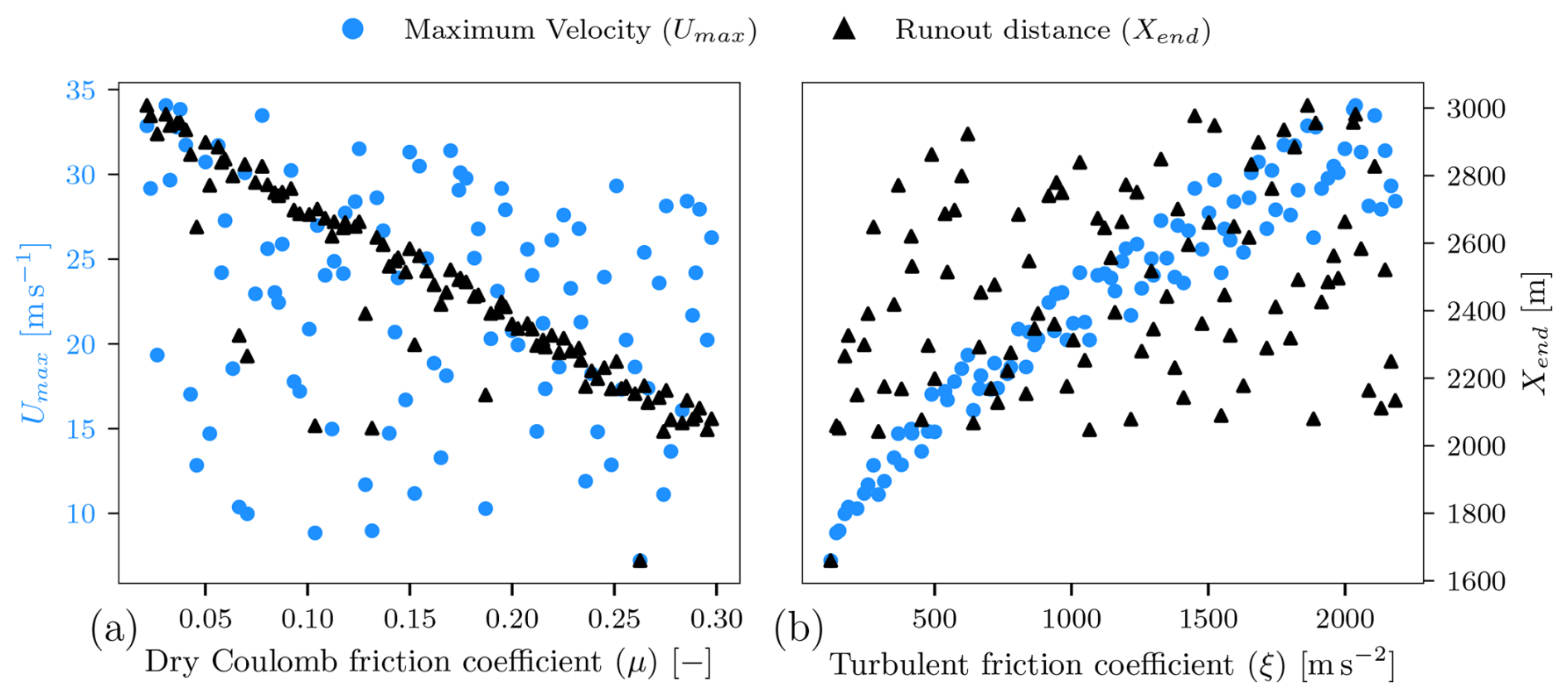
Figure 15 Variation of the friction coefficients (μ and ξ) with maximum velocity (U_max) and run out distance (X_end). The dry Coulomb friction coefficient μ primarily varies with X_end, while the turbulent friction coefficient ξ is more strongly influenced by U_max.

In numerical experiments 1 and 2, aggregated data proved inadequate in the joint calibration of the parameters – they could infer only one parameter each – we, therefore, explored time series data as an alternative. We calibrated the parameters using velocity and position time series data, each depicting the time history of velocity and position of the sliding mass, respectively. Figures 9 and 10 illustrate that the time series data provided substantial information during the calibration of both parameters, as evidenced by the highly contracted posteriors. This higher information gain implies that time series data are better equipped to calibrate friction parameters than aggregated data. Our findings are consistent with the work of Moretti et al. (2020), who observed that the time history data offered a better calibration of the landslide parameters than the static data. Specifically, the force-time history derived from seismic records was more adept at constraining landslide parameters than runout distance and deposit area because it captures the temporal evolution of landslide dynamics. In the same way, the velocity and position time series data used in our study captured the evolving dynamics of landslides more efficiently than aggregated data. A similar observation was made by Yan et al. (2022), who emphasized the limitations of static data in the adequate inversion of the landslide characteristics. Additionally, the friction parameters we want to calibrate govern the acceleration and deceleration phases of the landslide motion, which are better reflected in the time series data (Moretti et al., 2020). These findings further suggest that aligning observations with the critical process governed by the parameter of interest improves the calibration performance (Kavetski et al., 2011).

The superior performance of time series data compared to aggregated data implies a positive correlation between data quantity and calibration performance, where data quantity refers to the length and resolution of the time series. From Fig. 11, we can see that an increase in the length of time series leads to enhancement in calibration indicated by the contracting posteriors. Similarly, the calibration improves when we increase the temporal resolution, evidenced by posterior contraction with decreasing time step size, as shown in Fig. 13. These observations further support the claim that as the data quantity used for calibration increases, the calibration performance enhances accordingly. These observations echo findings in the field of hydrology, which highlight that increasing the data series length enhances the reliability of the calibration of a hydrological model (Cui et al., 2015; Li et al., 2010). Kavetski et al. (2011) reported similar findings; they compared the impact of the temporal resolution of the data on the calibration of the hydrological model parameters. They found that high-resolution data better captured parameters associated with fast hydrological processes, as these finer-scale data preserve the dynamics that are lost in coarser resolutions because of data averaging. However, more data does not necessarily lead to better calibration; for instance, Ekmekcioğlu et al. (2022) found that increasing the length of calibration data series beyond 10 years did not improve the validation performance of the hydrological model. Similarly, Etter et al. (2018) observed that the ability of the data to capture critical processes related to the parameters we want to calibrate was more critical than the temporal resolution of the data.

As the practical availability of data is often limited due to logistical and financial constraints (Seibert et al., 2024), we analyzed the information gained relative to the data points in the time series data. For this study, we calibrated friction parameters using multiple time series datasets, each containing several time steps. Figure 11 depicts the posterior distributions of the parameter ξ calibrated using a selected set of time series data of varying length. From Fig. 11, we can infer that as the number of time steps increases, the rate of information gain decreases, which implies that the ratio of information gain to the length of time series data is skewed after a certain threshold. This inference aligns with the study of Li et al. (2010), who found that the hydrological model calibration did not improve after a certain threshold, even with increased data series length. This inference is further reflected in Fig. 12a, where we plotted the information gain (quantified by KL divergence) against time steps. We can observe that the slope of this plot flattens after a certain threshold, indicating again that the rate of information gain diminishes after a threshold. We further observed from Fig. 12b that this threshold corresponds to an observation window in the velocity time series during which the sliding mass accelerates and attains its maximum velocity. Thus, this is the duration which marks the point at which the system's dynamics have evolved and stabilized, as critical processes affecting the dynamics have happened. Therefore, data capturing these changes is significantly more informative and relevant than the rest. This finding reinforces our earlier point: it is not solely the data quantity that matters, but rather its ability to capture the critical processes governing the parameters.

Beyond the insights from our synthetic case study, the proposed Bayesian data selection workflow provides a systematic framework for performing a priori assessment of data informativeness before costly field campaigns. To implement this framework, practitioners should first prepare a synthetic test case using site-specific topography and their computational model. By generating candidate observational datasets through forward model evaluation at known parameters, they establish a virtual testbed for scenario-based testing that quantifies how different candidate datasets inform specific parameters of interest and tests case-specific hypotheses about data value.

While we demonstrate the workflow using idealized topography and synthetic data, the model-agnostic approach can be transferred to complex models and real topographies. However, two practical limitations should be acknowledged. First, our statistical model assumes negligible model discrepancy – an assumption valid for synthetic data but potentially problematic when applying the framework to field observations where structural model inadequacies may prevent full explanation of the data. Second, when model misspecification or prior-data conflict occurs, posteriors can contract to incorrect regions of parameter space, where higher KL divergence does not necessarily indicate better calibration. This limitation is exacerbated when using non-uniform priors. For non-uniform priors, KL divergence between the posterior and the prior no longer reduces to posterior entropy alone, as it captures both the sharpness of the posterior and its shift from the prior distribution. This introduces a trade-off: when a posterior contracts to an incorrect region, KL divergence can assign high information gain to a misleading result because it rewards both concentration and shift. Conversely, entropy focuses solely on posterior sharpness and does not account for whether the posterior has shifted toward more plausible parameter regions. When applying this framework in such scenarios, practitioners should therefore complement these information-theoretic metrics with robust validation methods such as posterior predictive checks.

Figure 14a and b indicate that the discrepancy parameter is successfully calibrated using velocity and position time series. In this study, since we used synthetic data for calibration, we had control over the noise in the data; refer Sect. 2.1 and Table 1 for details. Specifically, we know the standard deviation of the Gaussian distribution from which the noise was drawn; for velocity time series, it was 2.08, and for position time series 225, see Sect. 3.2. These values closely align with the MAP estimates of the discrepancy parameter from the calibration of the velocity and position time series of 2.03 and 220, indicating our ability to infer this parameter and, thus, reflecting our ability to quantify the uncertainty associated with measurement noise. These findings further indicate that higher data quantity (like time series data) can help us quantify the uncertainty associated with the data quality. Our results are consistent with Khorashadi Zadeh et al. (2019), who reported that higher data quantity can offset the impact of poor data quality.

6 Conclusions

It is a well-known fact that the outcome of Bayesian calibration is highly dependent on the available observational data. However, there is a lack of studies that systematically investigate the impact of the selection of observation on the calibration result. We propose a Bayesian data selection workflow to address this challenge and identify the most informative observation in calibrating a given parameter. This workflow quantifies the impact of data selection on calibration performance by assessing the information gained during calibration, utilizing KL divergence, an established information-theoretic metric. Computing the KL divergence based on posterior distributions resulting from Bayesian parameter calibration presents itself as an extremely computationally intense task. We addressed the latter challenge by integrating a surrogate modeling technique based on GP emulation. The complete Bayesian data selection workflow is being made available with this article.

We have demonstrated the feasibility of the workflow through numerical experiments in which we systematically investigated the influence of data selection in calibrating two friction parameters of an idealized landslide runout model. To achieve this, we designed rigorous experiments that quantitatively assess how observations with variations in information content, specifically velocity versus position – and granularity, such as aggregated data versus time series data – affect the calibration outcome. The experimental results indicate that the information content and the observation granularity significantly impacted the calibration outcome. We found that time series data considerably outperforms aggregated data in constraining parameters, owing to its superior ability to capture the landslide dynamics. However, this does not imply that calibration performance scales linearly with the data quantity. While increasing the length and frequency of time series data enhances calibration performance, these improvements yield diminishing returns if the observation window exceeds a specific duration. Remarkably, the optimal length of the observation window that yields the maximum rate of information gain corresponds to the time the sliding mass needs to attain its maximum velocity. Thus, the evolution of landslide dynamics has stabilized. These findings suggest that data capturing the specific dynamics for an observation window of that duration are better suited to calibrate landslide model parameters. The landslide community can use these insights to optimize calibration strategies based on available data and to design effective future data acquisition strategies.

Appendix A

In this appendix section, we demonstrate that when using uniform priors, maximizing KL divergence between posterior and prior distributions is equivalent to minimizing the entropy of the posterior distribution.

Entropy of a random variable θ with probability distribution P(θ) is given as:

$$\begin{array}{}\text{(A1)}& H\left(P\right(\mathit{\theta }\left)\right)=-\int P\left(\mathit{\theta }\right)\log P\left(\mathit{\theta }\right)\mathrm{d}\mathit{\theta }\end{array}$$

KL divergence between the posterior and prior of a parameter θ calibrated using observation y is given as:

$$\begin{array}{}\text{(A2)}& D_{\mathrm{KL}}\left(P\right(\mathit{\theta }\mid y)\Vert P(\mathit{\theta }\left)\right)=\int P(\mathit{\theta }\mid y)\log \left({\displaystyle \frac{P(\mathit{\theta }\mid y)}{P\left(\mathit{\theta }\right)}}\right)\mathrm{d}\mathit{\theta }\end{array}$$

Expanding the logarithm, we obtain:

$$\begin{array}{}\text{(A3)}& \begin{array}{rl}& D_{\mathrm{KL}}\left(P\right(\mathit{\theta }\mid y)\Vert P(\mathit{\theta }\left)\right)=\int P(\mathit{\theta }\mid y)\left[\log P(\mathit{\theta }\mid y)-\log P\left(\mathit{\theta }\right)\right]\mathrm{d}\mathit{\theta }\\ & =\int P(\mathit{\theta }\mid y)\log P(\mathit{\theta }\mid y)\mathrm{d}\mathit{\theta }-\int P(\mathit{\theta }\mid y)\log P\left(\mathit{\theta }\right)\mathrm{d}\mathit{\theta }\\ & =-H\left(P\right(\mathit{\theta }\mid y\left)\right)-\int P(\mathit{\theta }\mid y)\log P\left(\mathit{\theta }\right)\mathrm{d}\mathit{\theta }\end{array}\end{array}$$

For a uniform prior over a bounded domain Θ with volume V, we have $P\left(\mathit{\theta }\right)=\frac{\mathrm{1}}{V}$ (constant). Substituting this:

$$\begin{array}{}\text{(A4)}& \begin{array}{rl}& D_{\mathrm{KL}}\left(P\right(\mathit{\theta }\mid y)\Vert P(\mathit{\theta }\left)\right)=-H\left(P\right(\mathit{\theta }\mid y\left)\right)-\int P(\mathit{\theta }\mid y)\log \left({\displaystyle \frac{\mathrm{1}}{V}}\right)\mathrm{d}\mathit{\theta }\\ & =-H\left(P\right(\mathit{\theta }\mid y\left)\right)+\log V\int P(\mathit{\theta }\mid y)\mathrm{d}\mathit{\theta }\\ & =-H\left(P\right(\mathit{\theta }\mid y\left)\right)+\log V\end{array}\end{array}$$

Thus KL divergence between the posterior and prior distributions reduces to the negative entropy of the posterior distribution plus a constant log (V), when using uniform priors. Therefore, selecting observations to maximize the KL divergence is equivalent to selecting observations that yield the sharpest posterior as discussed in Sect. 2.3.

Appendix B

In this appendix, we present trace plots of the MCMC chains from selected experiments (specifically experiments 1, 2, 3, 4, 7, and 8). The corresponding $\widehat{R}$ values are reported in Table B1. While the trace plots provide qualitative assessment of the convergence of the MCMC chains, $\widehat{R}$ values provides a quantitative measure of convergence (Vehtari et al., 2021).

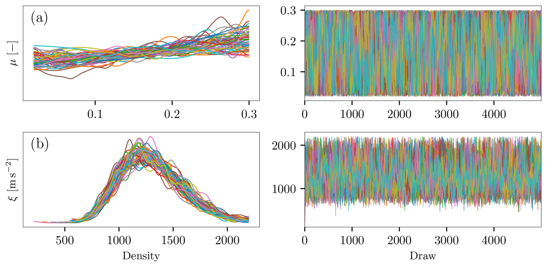
Figure B1 MCMC trace plots for (a) Dry Coulomb friction coefficient (μ) and (b) Turbulent friction coefficient (ξ) based on calibration with maximum velocity (U_max) as observation. Each color represents an independent chain. Left panels show kernel density estimates of the marginal posterior distributions. Right panels show trace plots across iterations, demonstrating chain convergence and adequate mixing.

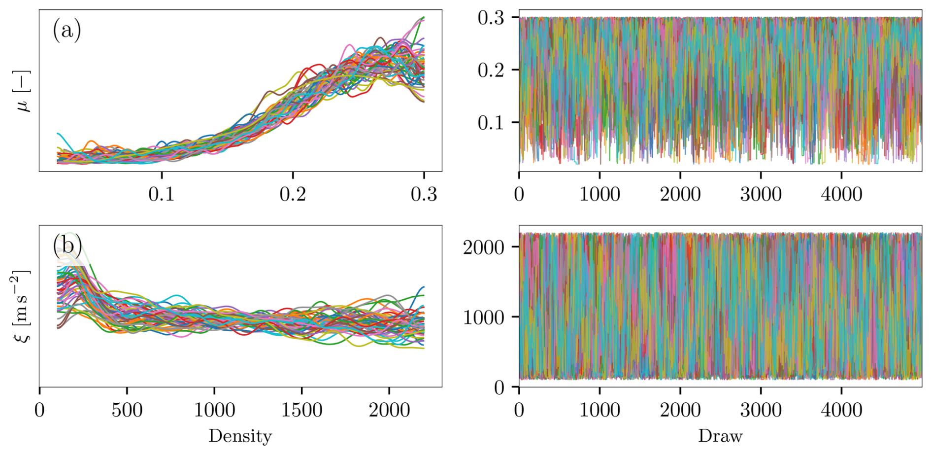
Figure B2 MCMC trace plots for (a) Dry Coulomb friction coefficient (μ) and (b) Turbulent friction coefficient (ξ) based on calibration with runout distance (X_end) as observation. Each color represents an independent chain. Left panels show kernel density estimates of the marginal posterior distributions. Right panels show trace plots across iterations, demonstrating chain convergence and adequate mixing.

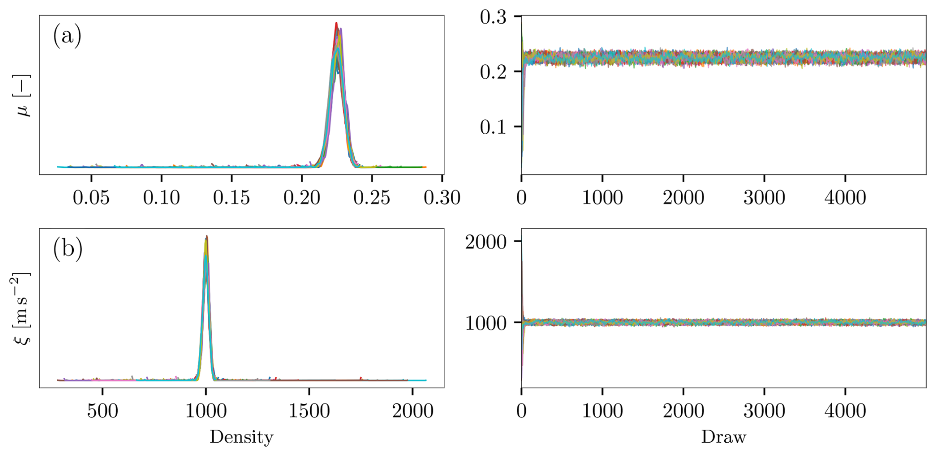
Figure B3 MCMC trace plots for (a) Dry Coulomb friction coefficient (μ) and (b) Turbulent friction coefficient (ξ) based on calibration with velocity time series as observation. Each color represents an independent chain. Left panels show kernel density estimates of the marginal posterior distributions. Right panels show trace plots across iterations, demonstrating chain convergence and adequate mixing.

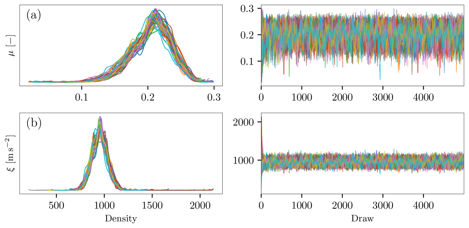
Figure B4 MCMC trace plots for (a) Dry Coulomb friction coefficient (μ) and (b) Turbulent friction coefficient (ξ) based on calibration with position time series as observation. Each color represents an independent chain. Left panels show kernel density estimates of the marginal posterior distributions. Right panels show trace plots across iterations, demonstrating chain convergence and adequate mixing.

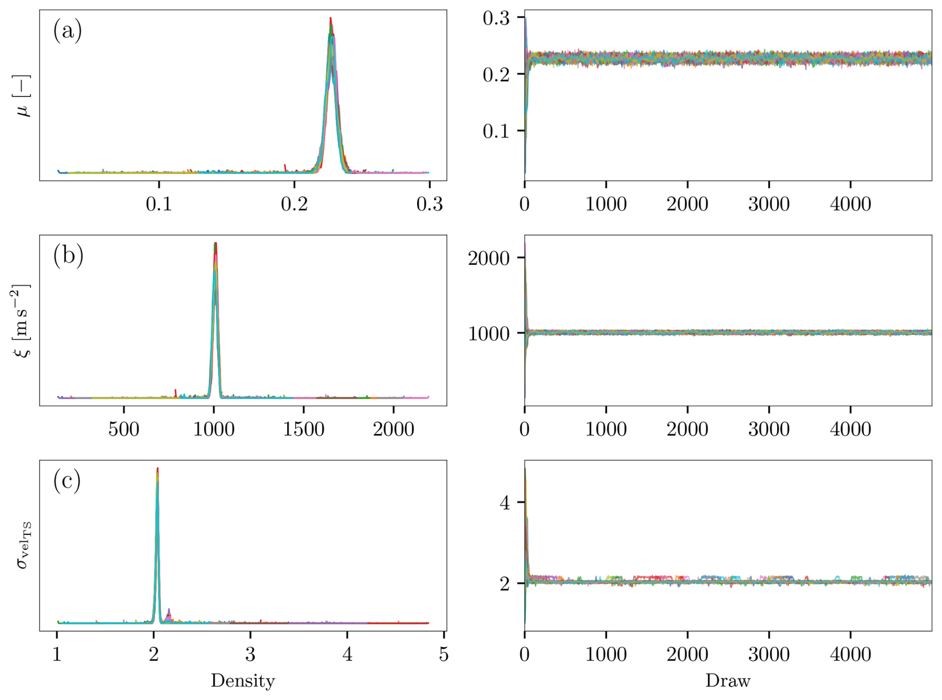
Figure B5 MCMC trace plots for (a) Dry Coulomb friction coefficient (μ) and (b) Turbulent friction coefficient (ξ) (c) Velocity discrepancy parameter $\left({\mathit{\sigma }}_{{\mathrm{vel}}_{\mathrm{TS}}}\right)$ based on calibration with velocity time series as observation. Each color represents an independent chain. Left panels show kernel density estimates of the marginal posterior distributions. Right panels show trace plots across iterations, demonstrating chain convergence and adequate mixing.

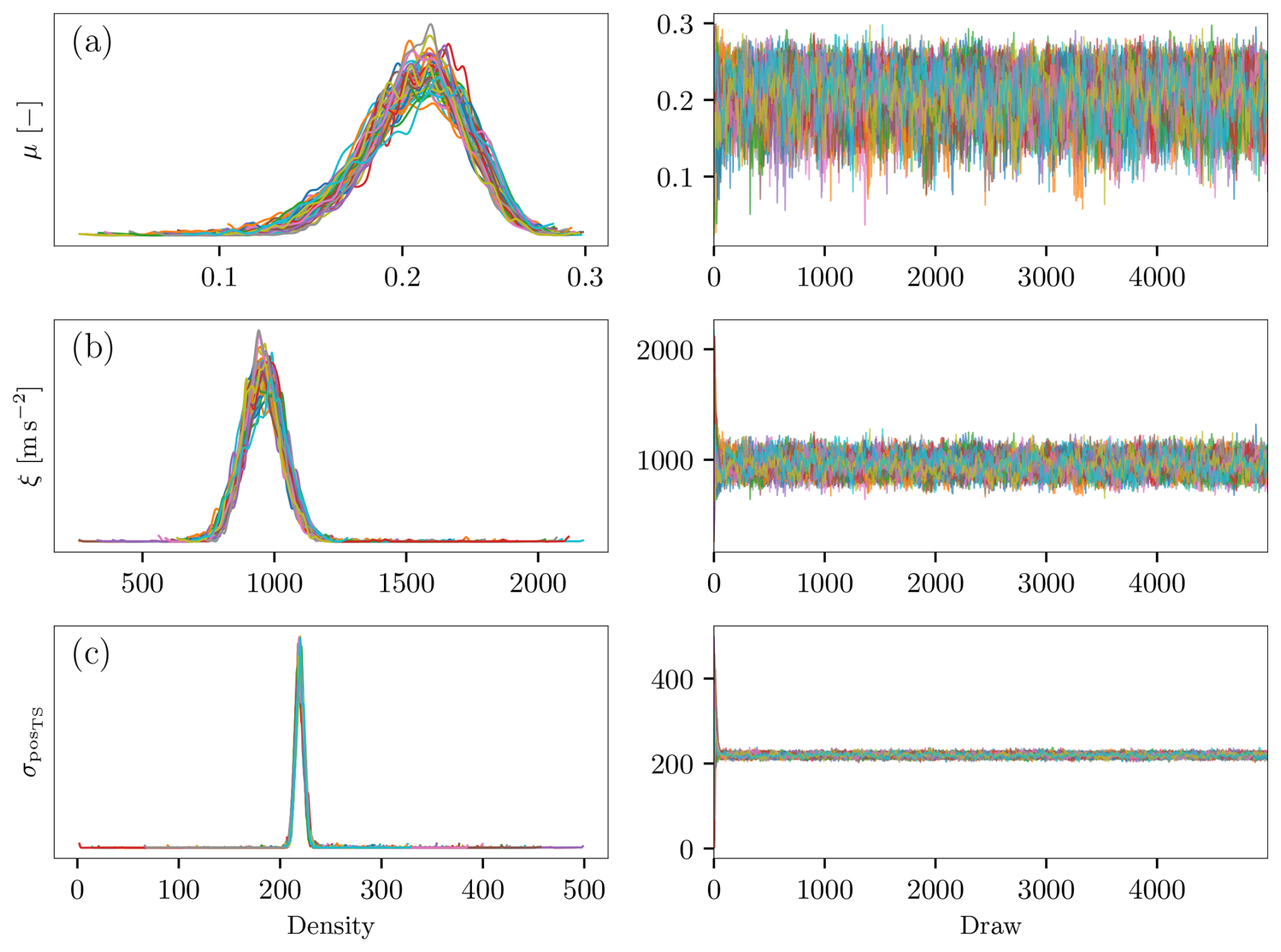
Figure B6 MCMC trace plots for (a) Dry Coulomb friction coefficient (μ) and (b) Turbulent friction coefficient (ξ) (c) Position discrepancy parameter $\left({\mathit{\sigma }}_{{\mathrm{pos}}_{\mathrm{TS}}}\right)$ based on calibration with position time series as observation. Each color represents an independent chain. Left panels show kernel density estimates of the marginal posterior distributions. Right panels show trace plots across iterations, demonstrating chain convergence and adequate mixing.

Table B1 Gelman-Rubin Statistic $\left(\widehat{R}\right)$ for MCMC sampling of friction coefficients and the discrepancy parameter. $\widehat{R}$ values indicate successful chain convergence for all parameters across different observations.

Appendix C

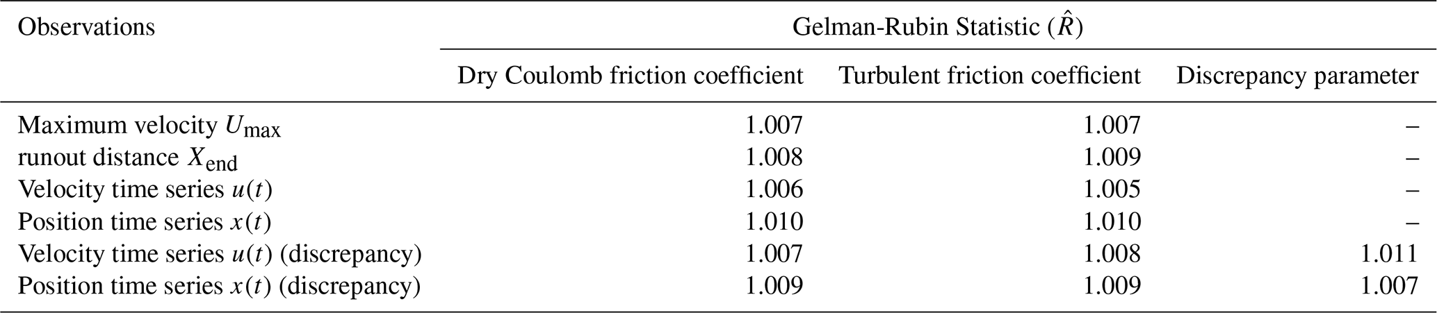
Figure 11 plots the posterior distributions of ξ calibrated with velocity time series datasets of increasing length. While information gain increases with time series length (reflected in progressively narrower posteriors), the differences between consecutive posteriors are much larger for initial time steps than for later ones, indicating a decreasing rate of information gain. To determine whether early time steps inherently contain more information, we performed calibration experiments using fixed-length observation time windows at different temporal positions. Figure C1 shows the posterior distributions of ξ calibrated using 100 time steps from observation windows positioned at: (0–100), (100–200), (200–300), (300–400), (700–800), (1000–1100), (1100–1200), and (1200–1300). This experimental setup allows direct comparison of information content across temporal positions. The results clearly show that posteriors become progressively wider for later time windows, confirming that initial time steps contain significantly more information about ξ than later time steps.

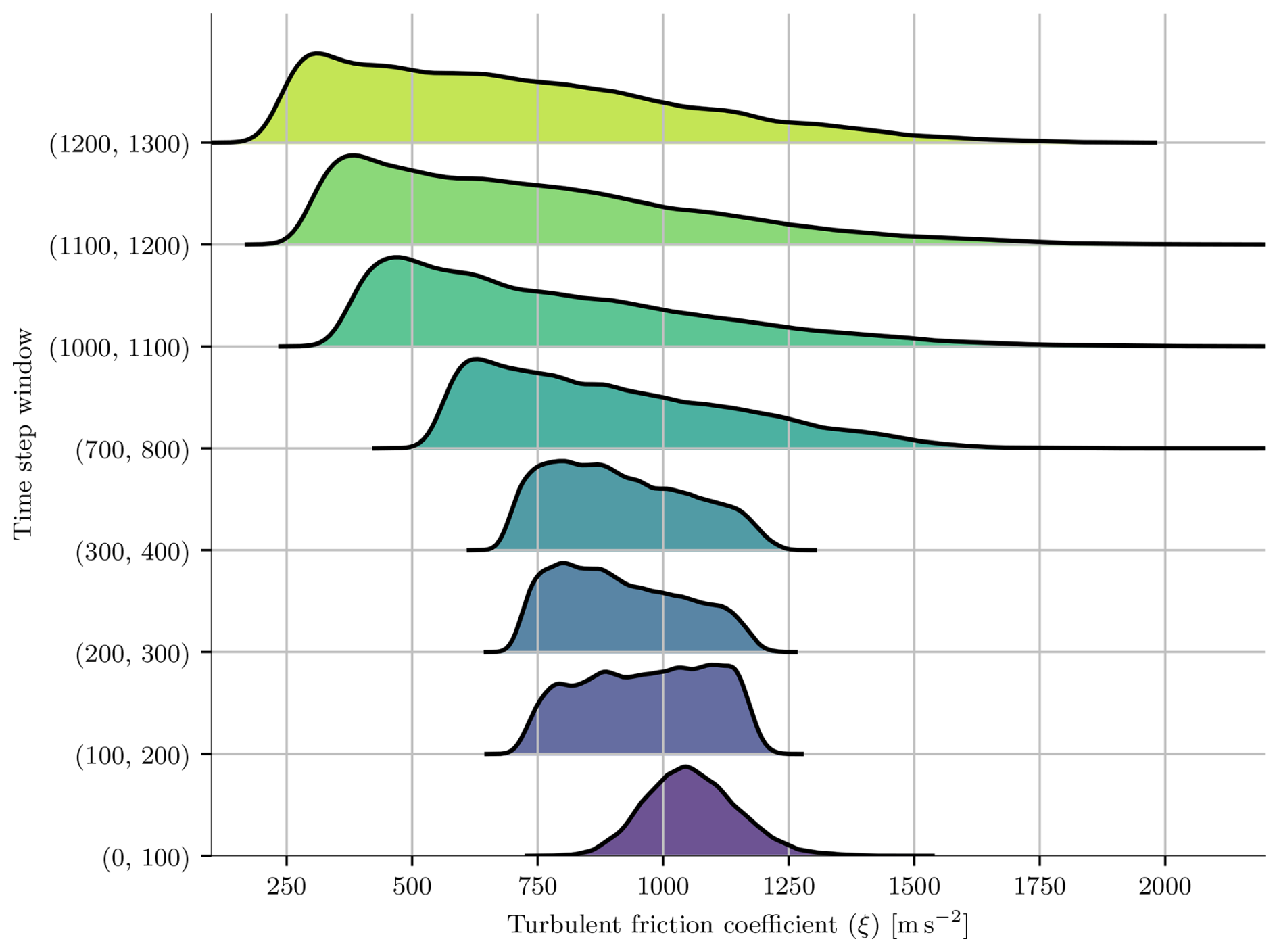
Figure C1 Posterior distributions of turbulent friction coefficient ξ calibrated with a fixed observation window of 100 time steps, with varying onset time. Initial time steps provide the highest information gain.