A simple dynamical system for representing climate tipping points with hysteresis

The risk that the climate system may contain tipping points remains a concern. Firstly, a level of global warming may be reached at which relatively small additional warming could cause major parts of the Earth system to transition to a new state. Depending on the location and specific Earth system component, this could disproportionately impact large sectors of society. Secondly, the Earth system component may exhibit hysteresis effects, and therefore, if global temperatures are subsequently lowered after triggering a jump in state, a return to earlier conditions may not occur until warming is substantially reduced. Earth System Models (ESMs) are numerical frameworks that operate at fine spatial scales. Such models are designed to estimate how all components of the climate system will evolve in response to changes in atmospheric greenhouse gas concentrations caused by human activity. Many ESM projections suggest that various parts of the climate system are capable of tipping. Yet, these models are computationally demanding and have therefore been operated only over a small range of scenarios. Very few “overshoot” simulations with ESMs exist, where climate change is reversed, resulting in limited understanding of hysteresis effects following a tipping event.

Advances in nonlinear mathematics include developing dynamical systems whose equations frequently contain a bifurcation parameter. These equations can accurately replicate tipping points, jumps in state, and hysteresis as the bifurcation parameter changes. Recent progress in ESM development often introduces higher spatial resolution, enhancing process representation and increasing accuracy in predicting local changes. However, mapping the broad behaviour of the components of ESM projections onto simpler dynamical system models may also offer many advantages, including the overall characterisation of climate models and a method to rapidly extrapolate their projections to a wider range of forcing scenarios. The bifurcation parameters in such equations may represent changing forcings, such as an increasing warming level that leads to a tipping event. Progress has already been made in mapping many components of the Earth system onto large-scale variables for representation as dynamical systems. Most advances to date have focused on understanding whether tipping events can be avoided if systems possess substantial inertia, i.e. respond over long timescales, allowing climate change to temporarily exceed thresholds that might otherwise trigger major nonlinear change. However, potential hysteresis effects in the context of climate change are less well represented in equation form. Achieving such a mathematical formulation requires a dynamic system to describe a climate system component not only at the point of tipping but also for substantial periods before and after. This behaviour corresponds to a bifurcation parameter that first increases and then decreases, with the modelled behaviours differing significantly during the return phase.

To support such necessary developments, we present a parameter-sparse dynamical system model that can exhibit hysteresis following a tipping occurrence, offering the potential for characterising Earth system components with this feature. We place particular emphasis on presenting in full the algebra needed to map known or modelled key attributes of a system that can tip onto the simplified dynamical system equation. We drive the equation with a time-evolving forcing representing an “overshoot” trajectory of global warming that exceeds a threshold for potential tipping. Calculations are performed over a range of system inertia values, illustrating a threshold inertia above which full tipping and hysteresis can be avoided. We use scale analysis to relate this threshold to those reported in existing climate research on behaviour near potential tipping points.

In some instances, a basic equation may be too simple to capture the dominant qualitative behaviour of a large-scale environmental system. In those cases, a more complex model from any hierarchy of suggested simulations of climate components may be appropriate. However, should a system be amenable to representation by a dynamical system, we hope the framework we present offers a simple-to-use equation structure that may quantify tipping points in the climate system. Such a framework may illustrate a more complete description of behaviours both before and after tipping, and depending on the post-tipping forcing scenario, it may involve substantial hysteresis.

1 Introduction

Climate tipping points represent critical thresholds, typically expressed as levels of global warming, beyond which positive feedbacks can cause components of the Earth system to irreversibly shift to a new state (Armstrong Mckay et al., 2022; Lenton et al., 2008, 2023; Abrams et al., 2023). Dansgaard–Oeschger events, observed in paleoclimate records, provide evidence of the capability of the Earth system to undergo such abrupt transitions (Boers, 2018; Buizert et al., 2024). With arguably insufficient progress being made on reducing human reliance on burning of fossil fuels, crossing climate tipping points in the near future is an increasingly likely scenario. Multiple generations of sophisticated climate models have displayed tipping behaviour in future climate scenarios (Drijfhout et al., 2015; Angevaare and Drijfhout, 2025). Examples include, but are not limited to, dieback of the Amazon rainforest (Melnikova et al., 2025; Parry et al., 2022), collapse of large scale circulation currents in the Atlantic Ocean (van Westen et al., 2024; Lohmann et al., 2024; Drijfhout et al., 2025; Loriani et al., 2025), melting of the polar ice sheets (Petrini et al., 2025; van den Akker et al., 2025) and alterations to atmospheric circulations (Loriani et al., 2025).

The tipping behaviour observed in these complex climate models (or complex ESMs) may be amenable to characterisation and replication by low-dimensional nonlinear dynamical systems (Dijkstra, 2013). Specifically, varying a parameter beyond a fold bifurcation can lead to bifurcation-induced tipping to an alternative state (Ashwin et al., 2012). However, if the parameter only temporarily exceeds a fold bifurcation, tipping of the system may not occur (Ritchie et al., 2021). The peak distance beyond the bifurcation and the duration of such an overshoot follow an inverse square law relationship, with the proportionality constant depending on the inertia of a system (Ritchie et al., 2019). A system with high inertia, such as large-scale ice sheets, is more likely to avoid tipping than a system with low inertia, such as coral reefs. This overshoot behaviour has been observed in both conceptual models (Ritchie et al., 2021) and complex climate models (Bochow et al., 2023). Policymakers are increasingly interested in considering the possibility of a climate overshoot (Huntingford and Lowe, 2007; Reisinger et al., 2025), which corresponds to a temporary period of warming above key target thresholds, after which temperatures are lowered back to those levels, potentially using engineering solutions. The “Paris Target” (UNFCCC, 2015) aims for society to limit global warming to 1.5 °C above pre-industrial levels. However, the temperatures recorded in recent years suggest that the planet may be very close to exceeding that threshold (Bevacqua et al., 2025), or may even be in the process of crossing it (Cannon, 2025). Hence, any final stabilisation at the 1.5° threshold is likely to occur after a temporary overshoot in global warming.

However, a second key attribute of tipping points, should they be activated and a rapid move to a new state occur, is the potential for hysteresis. This effect arises when lowering the forcing that initially triggered a tipping point may not result in a return to the pre-tipping state, and instead, the system remains locked in the new state. Hence, if a temporary period of warming overshoot causes a tipping point to occur, the reduction of temperatures after a peak level and back to below the tipping point threshold may not lead to a reversion to the states observed when temperatures were increasing. Proposed examples of hysteresis in the climate system include the potential behaviour of the oceanic thermohaline circulation (Rahmstorf et al., 2005), large-scale ice sheets (Garbe et al., 2020), the extent of mountain forest cover (Albrich et al., 2020), the level of tropical forest cover at key locations (Staal et al., 2020) and the position of the intertropical convergence zone (Kug et al., 2022). A broad summary of the climate attributes investigated for hysteresis, using one ESM that has been driven by a substantial ramp-up and ramp-down forcing in atmospheric CO₂ and thus global warming, is presented in Boucher et al. (2012). However, some quantities, such as mean local rainfall in many locations, may show little hysteresis when mapped against a global temperature profile that reverses (Walton and Huntingford, 2024). Understanding hysteresis requires a comprehensive assessment of a system that can tip, extending beyond merely quantifying its behaviour at the time or threshold of tipping. Instead, a more wide-scale analysis is needed to determine the importance of hysteresis by identifying how much temperatures may need to decrease before a return to initial states is achieved. Hence, capturing all these factors likely requires dynamical system models with more degrees of freedom and parameters than are needed to investigate the tipping point alone.

Yet, although there are more complexities in understanding a system that can both tip and exhibit hysteresis when driven by forcings with reversal, much can still be gained from identifying dynamical system models that can capture such behaviours. One key benefit is that if the mapping of a full-complexity system onto a simpler structure is believed to be robust and captures the broad features of a nonlinear component of the Earth system, it may be forced for an extended set of pathways. This enables calculations for a much broader range of potential futures, which are not possible to perform with full Earth System Models (ESMs) due to their heavy computational requirements. This possibility is especially important for “overshoot” scenarios, as very few ESMs have been routinely forced for such trajectories. A second advantage is that valid simpler models capture overall behaviours, often through their bulk parameters. Should a single simpler model be fitted to a range of ESMs, the resulting different parameter values provide a potentially concise way to quantify inter-ESM differences. In the context of tipping points, this may involve characterising warming thresholds for tipping, the size of the jump to an alternative state, and the level of global cooling required to avoid hysteresis and return to any initial state. A third advantage is that if more high-frequency variability is added to the simpler model, and it is found to interact with nonlinearities in a way that mimics features of ESMs, this may open a path to creating better early warning systems for approaching tipping elements. Developing early warning systems for climate tipping points remains an area of active research (Dakos et al., 2024) and discussion (Rietkerk et al., 2025). All of these advantages are possible if candidate dynamical system models are available for calibration against ESMs, both locally at tipping points and for their broader behaviours, including the period before tipping and any irreversibility (i.e. hysteresis) post-tipping.

Nonlinear mathematics has advanced substantially over recent decades (e.g. Enns, 2010), yielding sets of equations with bifurcation parameters (e.g. Kuznetsov, 2023). Upon adjustment of such parameters, these equations often exhibit simulated changes of state and irreversibility. Considerable progress has been made in mapping features of the climate system that are expected to have the potential to tip onto dynamical systems equations. The emphasis thus far has focused on studying the period when the system is near or at the tipping threshold. Specifically, theory has been developed (Ritchie et al., 2019) to understand whether, for some components of the Earth system, there is sufficient inertia to allow a temporary overshoot of a global warming level that, in equilibrium, would definitely cause tipping. Quantification of the possibility of inertia preventing tipping during a climate overshoot period has been undertaken for multiple parts of the Earth system (Ritchie et al., 2021, 2025).

To date, there has been far less progress in mapping the nonlinear behaviours of the Earth system onto dynamical systems when considering the full periods before and after tipping, or when tipping is averted due to inertia during temporary periods of high global warming. This omission is notable given the potential advances in understanding that could arise from such mappings. To bridge this gap, we present a relatively simple equation that exhibits tipping point and hysteresis effects. The particular novelty of our contribution lies in our explicit identification of key parameters that define a potential large-scale component of the climate system that exhibits such nonlinearity. The proposed system consists of five parameters: the level of global warming at which tipping occurs, the extent of the system at the point of tipping, a lower temperature representing the end of any hysteresis, the extent of the system at that lower temperature, and finally, a parameter defining inertia. A reader jumping to Eq. (7) will find a proposed dynamical system with the required properties. The equations shown before Eq. (7) allow a mapping of the parameters of the latter onto the five system-related parameters. Additionally, a reader can proceed to Eq. (16), which outlines a forcing trajectory in global warming. This trajectory consists of the historical period, smoothly transitioning into an idealised future “upturned” quadratic pathway, with the ability to set the peak warming level.

To support reproducibility, we replicate every step of the algebraic derivations, acknowledging that this makes the manuscript lengthy. We hope that this approach enables the analysis to serve as a valuable manual on how, starting from scratch, one can map Earth system components onto a potential descriptive dynamical system equation. This equation can then be used to explore tipping points, hysteresis, and inertial effects, as well as a range of potential global warming pathways, both with and without overshoot.

2 Mathematical model and parameterisation

Our aim is to provide an equation and a forcing profile capable of replicating a system that exhibits a tipping point, hysteresis behaviour, and inertia effects. We illustrate how the equation set may be calibrated (i.e. parameterised) and hope it will be useful to researchers wishing to quantify components of the Earth system believed to have strong nonlinear responses to climate change. Such beliefs may be driven by direct process understanding or based on assessments of projections by ESMs. We have aimed for a parameter-sparse model framework, but its development still requires substantial algebraic manipulations to illustrate how the main equations can be fitted to process knowledge. For full reproducibility, we have chosen to present all such algebra, though the majority of the background derivations are placed in the Appendix.

The paper leads to three main equations. Equation (7) describes the time-evolution of the Earth system component of interest, with the preceding algebra showing how to relate it to parameters that define an actual system. Equation (16) presents a representative future “overshoot” forcing profile in temperature, with the preceding algebra relating it to a prescribed maximum level of global warming and ensuring a smooth transition onwards from the historical record of global warming. Equation (24) provides a condition that differentiates whether, for the parameters provided, a system exhibits tipping and hysteresis, or if the warming trajectory instead avoids a change of state.

2.1 Mathematical model

Guided by a model of hysteresis to describe the Atlantic Meridional Overturning Circulation (AMOC) (e.g. van den Berk et al., 2021), we start with an equation of the form:

$$\begin{array}{}\text{(1)}& c_p^{\prime }{\displaystyle \frac{\mathrm{d}x}{\mathrm{d}t}}=-x^{\mathrm{3}}+\mathit{\beta }x+\mathit{\mu }.\end{array}$$

Here, x is a variable representing a changing component of the Earth system, which will be scaled to reflect the actual magnitude of this quantity. We consider μ as a bifurcation parameter whose value changes according to a metric of human-induced climate change. Metrics of climate change could include altered radiative forcing (W m⁻²), atmospheric carbon dioxide equivalent CO₂e (ppm), or global warming (K). Alternatively, if an attribute of the Earth system is strongly controlled by a regional and changing forcing from another part of the Earth system, then that attribute could instead determine the value of the evolving bifurcation parameter, μ. Here, t represents time (years) and $c_p^{\prime }$ is system inertia.

We set the bifurcation parameter as a linear function of the amount of global warming since the pre-industrial period, ΔT (K), as:

$$\begin{array}{}\text{(2)}& \mathit{\mu }={\mathit{\mu }}_{\mathrm{0}}+\mathit{\gamma }\mathrm{\Delta }T.\end{array}$$

Many use this form of “cubic” model (e.g. Eq. 1) to describe generic thermohaline circulations and often to better understand the effect of additional stochastic noise (e.g. Cessi, 1994), or to explain features of palaeo records (Boers et al., 2022). Boers (2021) investigates Early Warning Systems (EWSs) specific to the Atlantic Meridional Overturning Circulation (AMOC) by considering high-frequency variability combined with such a dynamical system. Recently, Wunderling et al. (2026) presented such a model to describe the risk of deforestation and related atmospheric feedbacks that may cause the remaining forest to also transition to grassland, with their detailed use of an illustrative dynamical system highlighted by Huntingford (2026). Coupled cubic dynamical systems are used to investigate the risk of cascading tipping points (Wunderling et al., 2021, 2023).

A more general analysis of the cubic form of a dynamical system with added noise is presented by Berglund and Gentz (2002). Similarly, Clarke et al. (2023), with such a dynamical system, consider whether EWSs designed to alert to approaching tipping may be made more accurate when accounting for any temporal autocorrelation in forcing. Ditlevsen and Johnsen (2010) illustrate, using such a model, that standard EWSs based on critical slowing down should be considered trustworthy only if both variance and autocorrelation increase. The difficulty of understanding equilibrium states that may be far from contemporary observations is shown by such a cubic dynamical system (Dakos and Kefi, 2022). Associated with tipping points are the mathematical properties of related EWSs that additionally entrain spatial variation. Clarke et al. (2026) consider cubic models at multiple locations with spatial connectivity, finding that, in some circumstances, accounting for spatial variation can produce more refined predictive statistics for distance to tipping. In some instances, a large scale process may be represented by a dynamical system, but it has to be more complex, potentially including more than one timescale (via parameter $c_p^{\prime }$) or more than one state variable, x, suggesting coupled equations. In some particular cases, the equations may contain switches, with behaviour conditional on the state variable or forcing level. However, the form of Eq. (1) in the literature, which describes many aspects of large-scale environmental change, is well established, and our aim here is to facilitate its application to further Earth system components when the values of key underlying defining attributes are known.

2.2 Calibration of equilibrium model

We first determine the equilibrium solutions of Eqs. (1) and (2) as a function of different mean global temperatures above pre-industrial levels, which we consider to be the bifurcation parameter. We set the system to have a tipping point at ΔT=ΔT_TP. The hysteresis is such that a return to earlier original states occurs at ΔT=ΔT_HYS. Hence, ΔT_HYS represents a second tipping point, and ΔT_TP−ΔT_HYS describes the width, in terms of global warming, over which hysteresis may occur. The quantity of interest, which is our state variable, is denoted as X, and is a scaled version of variable x. Our quantity of interest has a pre-industrial starting value of X=X_PI when ΔT=0 and has a bifurcation (tipping point) at X=X_TP when ΔT=ΔT_TP. Equilibrium solutions for higher temperatures beyond this point correspond to X being in a substantially different state.

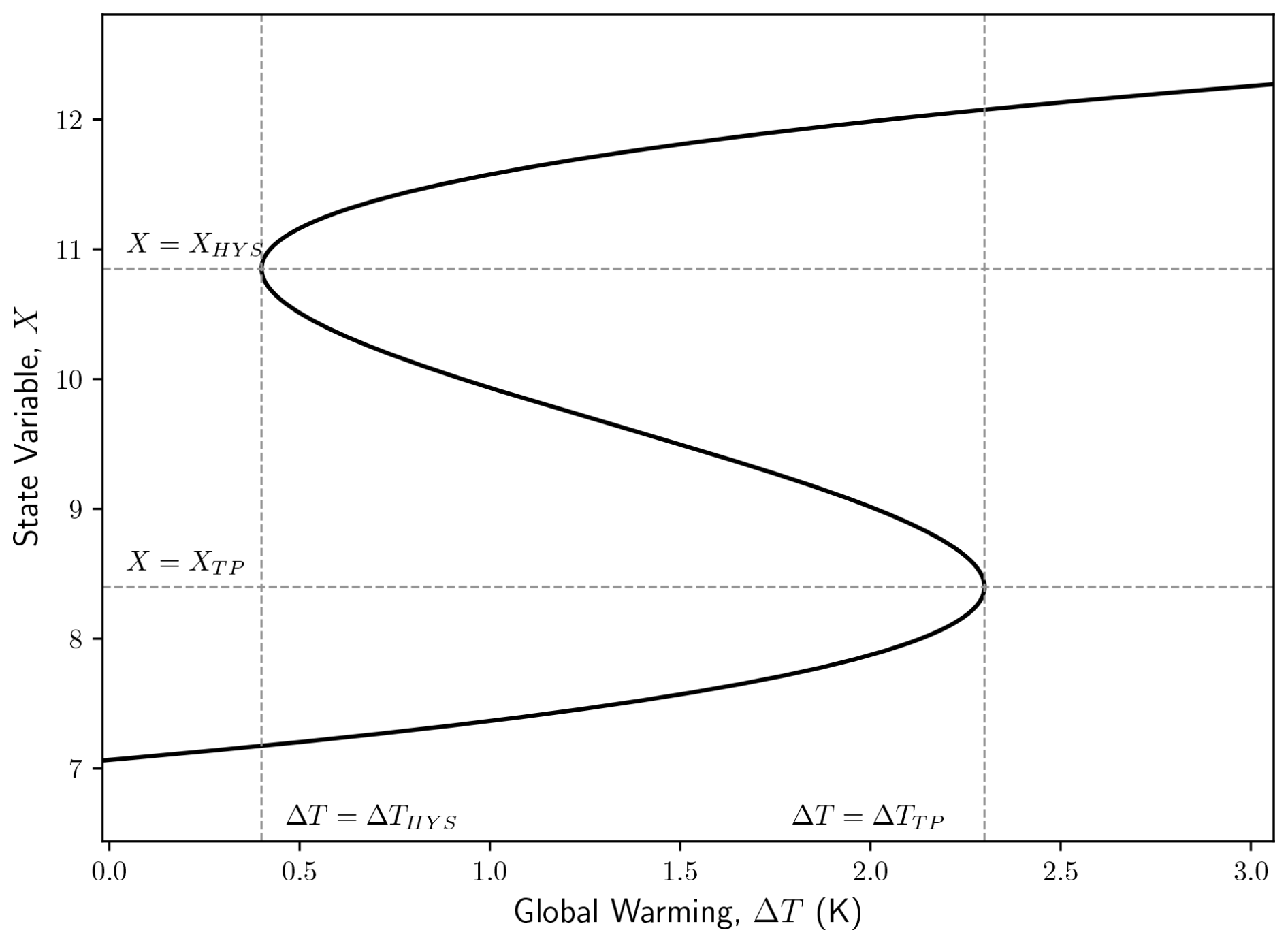
Figure 1 Equilibrium solutions to Eq. (7) for the tipping point defined at ΔT=ΔT_TP and X=X_TP, and for a second tipping point that marks the end of potential hysteresis for lowering temperatures at ΔT=ΔT_HYS and X=X_HYS. Equations (3)–(6) are used to derive values of $\mathit{\beta },{\mathit{\mu }}_{\mathrm{0}},a_{\mathrm{0}}$ and a₁, respectively, as needed in Eq. (7). These four parameters are functions of the prescribed values of $\mathrm{\Delta }{T}_{\text{TP}},X_{\text{TP}},\mathrm{\Delta }{T}_{\text{HYS}}$ and X_HYS used in this study. Additionally, vertical dashed lines are plotted independently at ΔT=ΔT_TP and ΔT=ΔT_HYS, as well as horizontal dashed lines at X=X_TP and X=X_HYS. The intersection of these lines at the tipping points provides visual verification of the algebra.

We initially seek the form of Eqs. (1) and (2) that align with the specification of the parameters set out above, as described in Appendix A. This gives an equation for β as

$$\begin{array}{}\text{(3)}& \mathit{\beta }={\left[{\displaystyle \frac{\mathrm{27}}{\mathrm{16}}}{\left(\mathrm{\Delta }{T}_{\text{TP}}-\mathrm{\Delta }{T}_{\text{HYS}}\right)}^{\mathrm{2}}\right]}^{\mathrm{1}/\mathrm{3}}\end{array}$$

and an equation for μ₀ as

$$\begin{array}{}\text{(4)}& {\mathit{\mu }}_{\mathrm{0}}=-{\displaystyle \frac{(\mathrm{\Delta }{T}_{\text{TP}}+\mathrm{\Delta }{T}_{\text{HYS}})}{\mathrm{2}}}.\end{array}$$

We map from the actual variable (i.e. quantity) of interest, X, which is in its physical units, to the variable x via a scaling of $x=a_{\mathrm{0}}+a_{\mathrm{1}}X$ (also shown as Eq. A7). From this we derive in Appendix A that a₁ and a₀ are given by

$$\begin{array}{}\text{(5)}& a_{\mathrm{1}}={\displaystyle \frac{\mathrm{2}}{(X_{\text{HYS}}-X_{\text{TP}})}}{\left[{\displaystyle \frac{\mathrm{\Delta }{T}_{\text{TP}}-\mathrm{\Delta }{T}_{\text{HYS}}}{\mathrm{4}}}\right]}^{\mathrm{1}/\mathrm{3}}\end{array}$$

and

$$\begin{array}{}\text{(6)}& a_{\mathrm{0}}=-\left({\displaystyle \frac{X_{\text{HYS}}+X_{\text{TP}}}{X_{\text{HYS}}-X_{\text{TP}}}}\right){\left[{\displaystyle \frac{\mathrm{\Delta }{T}_{\text{TP}}-\mathrm{\Delta }{T}_{\text{HYS}}}{\mathrm{4}}}\right]}^{\mathrm{1}/\mathrm{3}}.\end{array}$$

We can now write out the governing equation as a function of the state variable, X. Equations (1) and (2) may be combined, and with the scaling of Eq. (A7) and with γ=1, this gives:

$$\begin{array}{}\text{(7)}& c_p{\displaystyle \frac{\mathrm{d}X}{\mathrm{d}t}}=-(a_{\mathrm{0}}+a_{\mathrm{1}}X{)}^{\mathrm{3}}+\mathit{\beta }(a_{\mathrm{0}}+a_{\mathrm{1}}X)+({\mathit{\mu }}_{\mathrm{0}}+\mathrm{\Delta }T).\end{array}$$

Here, $c_p=a_{\mathrm{1}}{c}_p^{\prime }$, as a consequence of changing from the quantity x to X in the left-hand time derivative of Eq. (1).

We highlight Eq. (7) as it represents our dynamical system model in terms of the actual quantity of interest, X. Critically, using Eqs. (3)–(6), allows the four parameters of β, μ₀, a₁ and a₀ in Eq. (7) to be expressed as functions of the four user-defined quantities of ΔT_TP, ΔT_HYS, X_HYS and X_TP (this has a similarity to the recent approach taken by Couplet and Crucifix, 2025). The user can also specify c_p, which is a measure of system inertia. Additionally, the user can specify the bifurcation parameter and its changes, which here is global warming, ΔT, for which we explore different options in the sections below.

To provide a numerical example, we arbitrarily set the four defining parameters as ΔT_TP=2.3 K, ΔT_HYS=0.4 K, X_TP=8.4 (in units of X) and X_HYS=10.85 (units of X). With these values, we determine the equilibrium solution (or solutions) for X as a function of ΔT, corresponding to solving Eq. (7) with the left-hand side of that equation set to zero. These calculations are presented in Fig. 1. The algebra is also applicable if X_TP>X_HYS, and therefore valid for any system that tips downward, which could correspond to an event such as the shutdown of AMOC or the loss of rainforest cover in the Amazon.

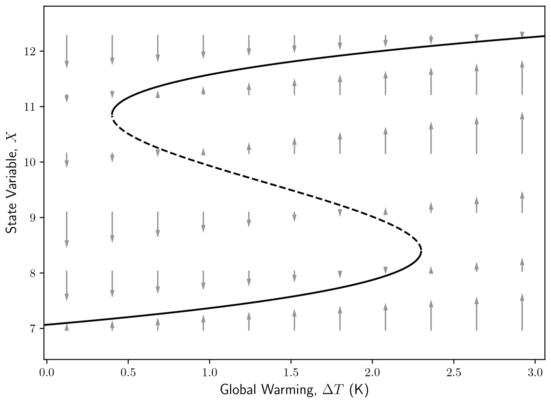
Figure 2 Transient solutions to Eq. (7) are examined for different but invariant values of the bifurcation parameter, ΔT, which here represents global warming. We adopt the same parameter values for $\mathrm{\Delta }{T}_{\text{TP}},\mathrm{\Delta }{T}_{\text{HYS}},X_{\text{TP}}$ and X_HYS as those used in Fig. 1. Additionally, we set c_p=50 (K year (X unit)⁻¹). Each arrow represents a solution to Eq. (7) with the starting point of the arrows defined by a set of initial conditions of X and ΔT, and where the latter remains fixed during each calculation. Equation (7) is solved in each example for a simulated period of 15 years, with the tip of the arrow indicating the final timepoint of the calculation. Retained from Fig. 1 is the presentation of the equilibrium solution, which is now subdivided into the stable part (continuous line) and the unstable part (dashed line).

2.3 Stability of equilibrium solutions with invariant bifurcation parameter

We first consider the temporal features of our model, without adjusting the bifurcation parameter, which implies keeping ΔT invariant. This scenario corresponds to a type of non-climatic forcing that adjusts our quantity X, after which it resets back towards a stable equilibrium state. We select a range of different initial states for X and ΔT, and from these, we solve Eq. (7), with the latter temperature variable fixed. We perform calculations for the same selection of values for $\mathrm{\Delta }{T}_{\text{TP}},X_{\text{TP}},\mathrm{\Delta }{T}_{\text{HYS}}$ and X_HYS, as used for the equilibrium solutions of Fig. 1. Additionally, we set the inertia to c_p=50 (K year (X unit)⁻¹). With these starting conditions and parameters, we solve for a period of 15 years using a simple explicit solver (calculating at 0.1 year timesteps). In Fig. 2, each arrow corresponds to a solution, with the beginning of the arrow representing the starting conditions and the end of the arrow indicating the final value derived after the simulated 15 year period. Hence, arrow length is representative of solution “velocity”.

2.4 Introduction of temporal forcing

We now consider a fully evolving system where the bifurcation parameter, representing global mean warming, adjusts over time. Such an approach extends our analysis, as well as that of other researchers (e.g. Couplet and Crucifix, 2025). We create time-evolving scenarios for future global warming, extending the known historical record since pre-industrial times. This extension is achieved by adding a quadratic temperature overshoot profile to the historical record. We adopt the global mean warming temperature record from NASA-GISS (NASA-GISS, 2025) as our historical record, which currently spans the years 1880–2024, setting t=0 for the year 1880. Also included in that timeseries data is a version that is smoothed in time (5 year lowess smoothing method; for details, see NASA-GISS, 2025), which forms the basis for the historical values we employ. We refer to this historical smoothed timeseries as ΔT_H,S(t). We use both the final values of that smoothed dataset and its gradient in time, leading up to the year $t=t^{+}=\text{2024–1880}$ (year), to initialise our parabolic curves of future warming.

We first normalise the NASA-GISS smoothed warming record such that it is zero when averaged across the period 1880–1900 inclusive, to give a timeseries ΔT(t). Hence,

$$\begin{array}{}\text{(8)}& \begin{array}{rl}{\displaystyle }\mathrm{\Delta }T\left(t\right)=& {\displaystyle }\mathrm{\Delta }{T}_{\text{H,S}}\left(t\right)-\mathit{ϵ}\mathrm{for}\mathrm{0}\le t\le t^{+}{t}^{+}=\mathrm{2024}-\mathrm{1880},\\ {\displaystyle }& {\displaystyle }\mathit{ϵ}={\stackrel{\mathrm{‾}}{\mathrm{\Delta }{T}_{\text{H,S}}\left(t\right)}}_{t=\mathrm{0}}^{t=\mathrm{21}}.\end{array}\end{array}$$

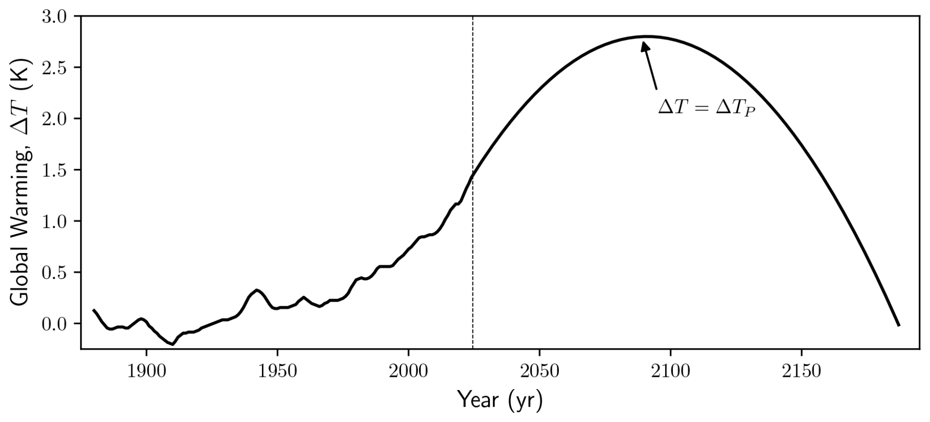
Figure 3 Historical record of global warming up to the year 2024, normalised so that the average of the first 21 years (1880–1900 inclusive) is zero. From the year 2024 onwards, a quadratic “overshoot” profile is derived, corresponding to setting an upper level of global warming of ΔT_P=2.8 K (as annotated). The vertical dotted line marks the year 2024. The future scenario is designed to transition smoothly from the historical measurement record in the year 2024.

We denote the final data value of ΔT, which is for the year 2024, as ΔT⁺. Additionally, we define the final gradient of that smoothing as the change between the years 2014 and 2024, which we divide by ten and name as δ (K yr⁻¹). Hence, the two contemporary boundary conditions are ϵ and δ at time $t=t^{+}$, expressed as:

$$\begin{array}{}\text{(9)}& {\displaystyle }& {\displaystyle }\mathrm{\Delta }{T}^{+}=\mathrm{\Delta }T\left(t^{+}\right),\text{(10)}& {\displaystyle }& {\displaystyle }\mathit{\delta }={\left.{\displaystyle \frac{\mathrm{d}\mathrm{\Delta }T}{\mathrm{d}t}}\right|}_{t=t^{+}}.\end{array}$$

We calculate the coefficients for a quadratic overshoot function to smoothly extend the historical dataset by satisfying the boundary conditions given in Eqs. (9) and (10). The quadratic form then proceeds to a user-prescribed maximum value of global warming, ΔT_P, before declining. The quadratic form of future warming is defined as

$$\begin{array}{}\text{(11)}& \mathrm{\Delta }{T}^{*}=e{t}^{{*}^{\mathrm{2}}}+f{t}^{*}+g\end{array}$$

We initially seek the form which incorporates offsets in time and warming as

$$\begin{array}{}\text{(12)}& t^{*}=t-t^{+},\mathrm{\Delta }{T}^{*}\left(t^{*}\right)=\mathrm{\Delta }T\left(t\right)-\mathrm{\Delta }{T}^{+}.\end{array}$$

Thus, $t^{*}=\mathrm{0}$ (yr) and $\mathrm{\Delta }{T}^{*}=\mathrm{0}$ (K) at the transition time, i.e. year 2024, moving from the historical record to the future warming scenario. In Appendix B we derive values for g as

$$\begin{array}{}\text{(13)}& g=\mathrm{0},\end{array}$$

for f as

$$\begin{array}{}\text{(14)}& f=\mathit{\delta },\end{array}$$

and for e as

$$\begin{array}{}\text{(15)}& e={\displaystyle \frac{-{\mathit{\delta }}^{\mathrm{2}}}{\mathrm{4}\left(\mathrm{\Delta }{T}_{\mathrm{P}}-\mathrm{\Delta }{T}^{+}\right)}}.\end{array}$$

Removing the offsets of Eqs. (12) in Eq. (11), then in terms of global warming, ΔT, and time, $t-t^{+}$, the future projection for years following the end of the historical dataset (i.e. $t-t^{+}\ge \mathrm{0}$) is given by the key equation:

$$\begin{array}{}\text{(16)}& \mathrm{\Delta }T=e(t-t^{+}{)}^{\mathrm{2}}+f(t-t^{+})+g+\mathrm{\Delta }{T}^{+},\end{array}$$

with e, f and g given by Eqs. (15), (14) and (13) respectively. Hence, the quadratic future temperature trajectory parameters are a function of the historical timeseries leading to it, described by parameters ΔT⁺ and δ, along with the user-defined peak warming, ΔT_P. We regard the end of the extended timeseries as the year in which the quadratic function returns to zero global warming.

For our numerical calculations, we extend our historical record and calculate a future temperature trajectory using the boxed Eq. (16), with a maximum level of global warming of ΔT_P=2.8 K. Both the historical record and the future trajectory are shown in Fig. 3.

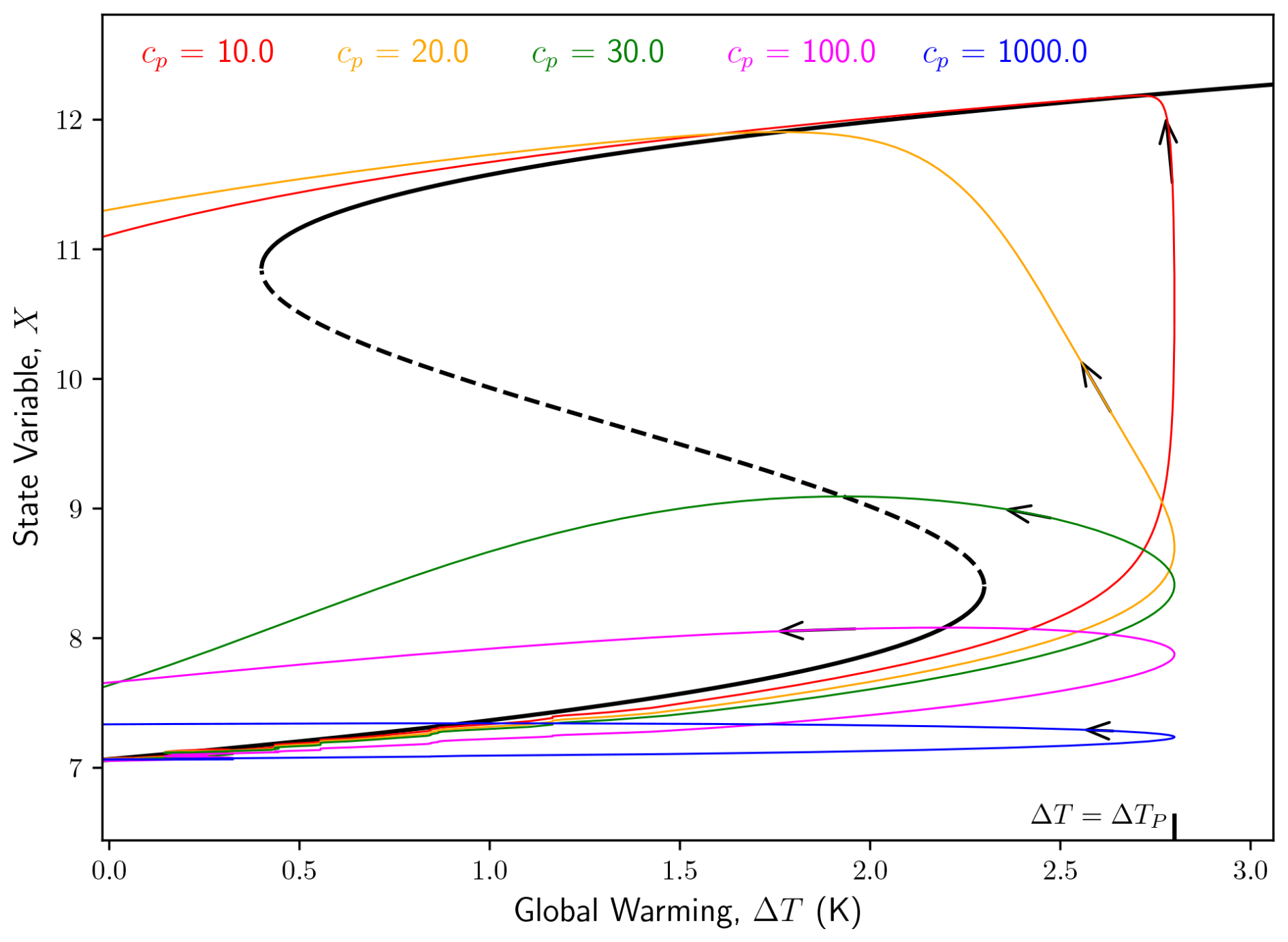
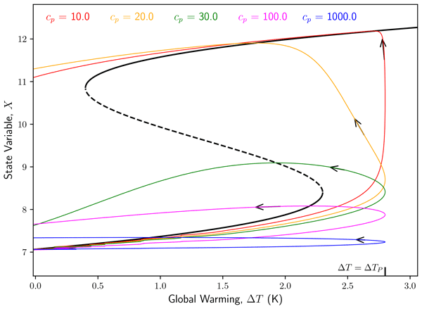
Figure 4 Transient simulations are described by Eq. (7) and conducted with a forcing of global warming ΔT given by Eq. (16). The global warming driver is considered to change the bifurcation parameter. In all calculations, the initial condition to Eq. (7) is that at the year 1880 (and so when ΔT=0), the value of X is the equilibrium solution. Calculations are performed for different values of c_p, as marked by different colours and the legend. Small black arrows illustrate the direction, in time, of the phase curves. The axes are identical to those of Figs. 1 and 2. The equilibrium solutions are retained from Fig. 2, as shown by the black continuous and dashed lines. The maximum, i.e. peak level of global warming, in all five transient simulations is at $\mathrm{\Delta }T=\mathrm{\Delta }{T}_{\mathrm{P}}=\mathrm{2.8}\mathrm{K}$, as indicated by the inward tick mark on the “x” axis.

2.5 Full model simulations with time-varying global warming

We investigate our model of tipping point behaviour when including full transient effects. The complete model is given by Eq. (7) combined with our timeseries of global warming described by Eq. (16). It is recalled that in this model framework, we regard global warming, ΔT, as the bifurcation parameter. Simulations of this ordinary differential equation setup are initialised with the pre-industrial levels of X at equilibrium. Specifically, the initial condition for all our calculations in the simulated year 1880 is the solution to Eq. (7) with both the time derivative term and ΔT set to zero. For the parameters we use (i.e. $\mathrm{\Delta }{T}_{\text{TP}},\mathrm{\Delta }{T}_{\text{HYS}},X_{\text{HYS}}$ and X_TP), this common value in the first year, t=0, of all simulations in Fig. 4, is X_PI=7.06. Five calculations are performed, corresponding to different and increasing inertia values, c_p (K yr [unit of X]⁻¹). A simple explicit solver is used again, with a timestep of 0.1 years.

Each simulation covers the full historical period plus the future time period of global warming overshoot, as shown in Fig. 3. For the lowest inertia of c_p=10 (Fig. 4, red curve), around the time of maximum warming (i.e. ΔT reaches ΔT_P), the solution “tips” and moves directly to the equilibrium solution at a higher X. At the next highest inertia of c_p=20, (Fig. 4, orange curve), the solution also moves to the higher value of X, but takes longer to do so after the peak warming. In both these cases, the solution will tip back to the starting branch (given sufficient time) since global warming drops below the lower fold bifurcation ΔT_HYS=0.4 K. At the next test value of c_p=30, (Fig. 4, green curve), the solution makes an extensive excursion towards the higher equilibrium solution, but eventually returns towards the initial state for the period simulated. For c_p=100, (Fig. 4, magenta curve), there is a similarity to that of the green curve, except that the excursion towards the upper equilibrium solution is much more limited. In the final calculation, with c_p=1000 (Fig. 4, blue curve), at this very high level of inertia, the solution exhibits very little variation in X.

2.6 Mathematical analysis

We now mathematically study the governing equation Eq. (7), forced by a potential overshoot scenario of future global temperature as set out in the quadratic form of Eq. (16). Our goal in this section is to understand the factors that determine whether, when temperatures overshoot the tipping threshold, the system exhibits a relatively small excursion in X before returning towards the initial state (blue, pink, and green curves in Fig. 4) or instead follows a full hysteresis loop (yellow and red curves). In particular, we are interested in the role that inertia of the system, quantified by c_p, plays in determining which of these cases occurs.

To understand the relative importance of different aspects of the system, we convert the equations into a non-dimensional form. Such a mapping often shows more clearly how different combinations of parameters affect the dynamics. We introduce shifted X and t variables, denoted as y and τ respectively, defined as:

$$\begin{array}{}\text{(17)}& y={\displaystyle \frac{a_{\mathrm{0}}+a_{\mathrm{1}}X}{a_{\mathrm{1}}\widehat{X}}},\mathit{\tau }={\displaystyle \frac{t-t^{+}}{\widehat{t}}}.\end{array}$$

Here, $\widehat{X}$ and $\widehat{t}$ are characteristic values of the X and t quantities, and so by construction, y and τ are dimensionless variables. We set these two new variables to obtain a nondimensional system that is as simple as possible, with the full derivation given in Appendix C. With

$$\begin{array}{}\text{(18)}& \widehat{t}={\displaystyle \frac{c_p}{\mathit{\beta }{a}_{\mathrm{1}}}}\end{array}$$

and

$$\begin{array}{}\text{(19)}& \widehat{X}={\displaystyle \frac{\sqrt{\mathit{\beta }}}{a_{\mathrm{1}}}}\end{array}$$

this results (see Appendix C) in

$$\begin{array}{}\text{(20)}& {\displaystyle \frac{\mathrm{d}y}{\mathrm{d}\mathit{\tau }}}=-y^{\mathrm{3}}+y+{\mathit{\pi }}_{\mathrm{0}}+{\mathit{\pi }}_{\mathrm{1}}\mathit{\tau }+{\mathit{\pi }}_{\mathrm{2}}{\mathit{\tau }}^{\mathrm{2}}.\end{array}$$

with the three nondimensional parameter clusters π₀,π₁ and π₂ equal to:

$$\begin{array}{}\text{(21)}& {\displaystyle }& {\displaystyle }{\mathit{\pi }}_{\mathrm{0}}={\displaystyle \frac{\mathrm{2}\sqrt{\mathrm{3}}}{\mathrm{9}}}\left({\displaystyle \frac{\mathrm{2}\mathrm{\Delta }{T}^{+}-\mathrm{\Delta }{T}_{\text{HYS}}-\mathrm{\Delta }{T}_{\text{TP}}}{\mathrm{\Delta }{T}_{\text{TP}}-\mathrm{\Delta }{T}_{\text{HYS}}}}\right),\text{(22)}& {\displaystyle }& {\displaystyle }{\mathit{\pi }}_{\mathrm{1}}={\displaystyle \frac{\mathrm{8}{c}_p\mathit{\delta }\sqrt{\mathrm{3}}}{\mathrm{27}}}\left({\displaystyle \frac{X_{\text{HYS}}-X_{\text{TP}}}{(\mathrm{\Delta }{T}_{\text{TP}}-\mathrm{\Delta }{T}_{\text{HYS}}{)}^{\mathrm{2}}}}\right),\text{(23)}& {\displaystyle }& {\displaystyle }{\displaystyle }{\mathit{\pi }}_{\mathrm{2}}=-{\displaystyle \frac{\mathrm{4}\sqrt{\mathrm{3}}{c}_p^{\mathrm{2}}{\mathit{\delta }}^{\mathrm{2}}}{\mathrm{81}}}\times \left({\displaystyle \frac{(X_{\text{HYS}}-X_{\text{TP}}{)}^{\mathrm{2}}}{(\mathrm{\Delta }{T}_{\mathrm{P}}-\mathrm{\Delta }{T}^{+})(\mathrm{\Delta }{T}_{\text{TP}}-\mathrm{\Delta }{T}_{\text{HYS}}{)}^{\mathrm{3}}}}\right).\end{array}$$

The analysis presented in Appendix C leads to an inequality. If this inequality is satisfied, then although the warming threshold for potential tipping is temporarily crossed, the jump to a new state is not achieved, and no major related hysteresis occurs. This inequality is given by the key equation

$$\begin{array}{}\text{(24)}& {\mathit{\pi }}_{\mathrm{0}}\le {\displaystyle \frac{\mathrm{1}}{\mathrm{4}}}{\displaystyle \frac{{\mathit{\pi }}_{\mathrm{1}}^{\mathrm{2}}}{{\mathit{\pi }}_{\mathrm{2}}}}+{\displaystyle \frac{\mathrm{2}}{\mathrm{3}\sqrt{\mathrm{3}}}}+\sqrt{-{\displaystyle \frac{{\mathit{\pi }}_{\mathrm{2}}}{\sqrt{\mathrm{3}}}}}\end{array}$$

and is the same threshold, but in our notation, as in Ritchie et al. (2019). This inequality is expected to be broadly valid for a range of temperature overshoots, not just those that are asymptotically small. Finally, we can evaluate this inequality. Substituting the parameter choices that lead to Fig. 4 into Eqs. (21)–(23), while retaining the dependence on inertia, c_p, gives:

$$\begin{array}{}\text{(25)}& \begin{array}{rl}{\displaystyle }& {\displaystyle }{\mathit{\pi }}_{\mathrm{0}}\approx \mathrm{0.03241},{\mathit{\pi }}_{\mathrm{1}}\approx \mathrm{0.01428}{c}_p,\\ {\displaystyle }& {\displaystyle }{\mathit{\pi }}_{\mathrm{2}}\approx -\mathrm{9.18447}\times {\mathrm{10}}^{-\mathrm{5}}{c}_p^{\mathrm{2}}.\end{array}\end{array}$$

Inserting these Eqs. (25) into the inequality Eq. (24) reveals that, for a temporary overshoot to avoid full tipping and hysteresis, requires inertia sufficiently large that c_p≥27.8, which is in good agreement with Fig. 4.

3 Discussion and conclusions

The risk of triggering tipping points in major parts of the Earth system remains a key concern regarding potential responses to a changing climate as atmospheric greenhouse gases increase. Tipping refers to a shift of an Earth system component to a new state, which may occur with relatively little additional climate change. This new state may also exhibit hysteresis, implying that any attempt to reverse climate change after tipping might not restore the system to its original state. Research centres have contributed Earth System Models (ESMs) to the Climate Model Intercomparison Project version 6 (Eyring et al., 2016; Tebaldi et al., 2021), which inform the IPCC reports IPCC (2021). ESMs predict various tipping points, but there is little consensus among these models about the level of climate change that would trigger their activation. Moreover, specific tipping points do not necessarily appear in all ESMs. To characterise the simulated tipping points, they should ideally be mapped onto a common equation framework, with parameters aligned to each ESM. Such equations may also enable the investigation of additional possible climate change trajectories for which ESMs have not been operated.

We begin with a moderately basic nonlinear ordinary differential equation, Eq. (1), which exhibits tipping point and hysteresis effects. This equation, of “cubic” form, has been proposed by many to describe features of the Earth system (see Sect. 2.1 for references), but there is presently no routine method to describe how to map climate tipping point features onto this model. To do this, we use a variable X to represent our system state, denoting a component of the Earth system of interest. We assume that four quantities are available to define the background equilibrium states, either already known (e.g. estimated from palaeo data) or obtained from more complex ESM calculations. These parameters include the value of X at tipping, X_TP, and the global warming temperature at which it occurs, ΔT_TP. The other two parameters are the value of X at the end of hysteresis, X_HYS, and the corresponding lower global warming temperature at which it occurs, ΔT_HYS. These four parameters are illustrated in Fig. 1.

The particular form of the governing equation that we propose is our key process Eq. (7). If we initially neglect the transient left-hand-side term (by setting it to zero), the remaining equation describes the pseudo-equilibrium solutions for various values of global warming, ΔT. In this context, the assumption is that there are very slow palaeo-timescale changes in ΔT, which we consider as a bifurcation parameter. The right-hand side of Eq. (7) involves four unknown parameters, $\mathit{\beta },{\mathit{\mu }}_{\mathrm{0}},a_{\mathrm{0}}$ and a₁. These parameters are functions of our four user-defined parameters, $X_{\text{TP}},\mathrm{\Delta }{T}_{\text{TP}},X_{\text{HYS}}$ and ΔT_HYS, as specified by Eqs. (3)–(6).

We introduce transient effects into our calculations in two ways. We assume that the system simulated by the variable X has inertial effects, which we represent by a fifth user-defined parameter, c_p, in Eq. (7). Then we introduce a time-evolving profile for global warming, ΔT(t), which combines the historical record with a future “overshoot” scenario that we model as quadratic. The three quadratic coefficients are partially constrained by the magnitude (ΔT⁺) and the rate of change of warming (δ) for the contemporary period, thereby ensuring a smooth transition from the warming of the recent past to that of the simulated future. The required third constraint is a user-prescribed value for the peak level of global warming, ΔT_P. This warming profile leads to our second key equation, Eq. (16), as illustrated in Fig. 3 and for our value of ΔT_P=2.8. The three parameters of $\mathrm{\Delta }{T}^{+},\mathit{\delta }$ and ΔT_P are translated into the three parameters e,f and g, given by Eqs. (15), (14) and (13) respectively.

Our second aim is to investigate and characterise solutions to Eqs. (7) and (16) for a range of inertial values, c_p, in response to human-induced climate change. The focus on an overshoot warming profile is deliberate, as it allows us to consider the potential for hysteresis should a tipping point be activated and there is a reversal of forcing. If society achieves eventual climate stabilisation at a global warming level of 1.5 or 2 °C above pre-industrial levels, this may occur after a temporary period of higher global temperatures. Such an overshoot is possible, given that current emissions levels may not be falling sufficiently fast to allow the climate system to approach a stabilisation maximum temperature only from below. Using numerical calculations, we find that for high inertia, the variable X will not exhibit major tipping and hysteresis (Fig. 4). Employing the nondimensionalisation method to our model and forcing equations, we estimate with Eq. (24) a threshold that determines whether tipping can be avoided. These calculations relate to existing analysis (e.g. Ritchie et al., 2019, 2021, 2025) that estimates the risk of tipping when the equilibrium level for activation is temporarily crossed. If there is additional understanding leading to a known value of c_p, then the model equation, Eq. (7), is fully constrained by process knowledge.

Equation (7) is available to assess responses to forcings of alternative future trajectories in global warming, ΔT. Our quadratic form, which we consider as eventually returning to pre-industrial conditions, may be replaced with more sophisticated profiles that stabilise at key warming thresholds, either with or without a period of overshoot. Algebraic forms exist for such profiles (e.g. Huntingford et al., 2017), opening the possibility of further analytic assessment, again without relying solely on numerical understanding. The equation system is also available for forcing with monotonically increasing global temperatures, which is likely to occur during the 21st Century if society follows any of the standard Shared Socioeconomic Pathways (SSPs) (Riahi et al., 2017) that are associated with the continued substantial burning of fossil fuels.

Due to concerns that human-induced climate alteration may cause key components of the Earth system to tip, there is substantial interest in developing early warning systems for such events (e.g. Dakos et al., 2024). Although generic types of such warning systems exist, such as those that assess for evidence of critical slowing down, more bespoke forms may be developed for particular parts of the climate system. We suggest that a calibrated dynamical system, which accurately describes a key process, could also support the development of such warning systems. For instance, adding high-frequency noise to Eq. (7), either to ΔT or X, and studying the simulated responses and how they change as tipping approaches, may lead to the discovery of more accurate warning methods.

Our analysis has some caveats. The generic cubic form, in X, of the right-hand side of Eq. (7), to some extent, predetermines any path taken by the state variable in the presence of hysteresis. The actual components of the climate system may exhibit slightly different forms, necessitating more complex algebraic expressions that introduce perturbation terms to the cubic structure. In addition, utilising the normal form and a linear change in variables assumes a certain symmetry to the problem, for example, as seen in Fig. 1. At the midpoint between the folds of ΔT_HYS and ΔT_TP the distances to the basin boundary (the middle unstable branch), from the stable top and lower branches, are the same. However, some problems might require a nonlinear coordinate change, which could lead to asymmetric basins of attraction. The equations we provide model only a single state variable, X, while there is concern that the activation of a tipping point may alter the timing of others, creating a cascade effect. A suggested set of equations that captures such effects, along with their couplings, is provided by Wunderling et al. (2021). In our modelling framework, we only consider the passage through fold bifurcations. However, tipping can arise from oscillatory instabilities, which are often attributed to passing through a Hopf bifurcation. Or, alternatively, tipping can even occur without crossing any bifurcations via rate-induced tipping, such as those attributed to peatland fires (Clarke et al., 2021).

In summary, we provide a relatively simple equation on to which the behaviour of climate components expected to exhibit a tipping point, leading to a new state, can potentially be mapped. The equation can simulate hysteresis effects. Given the interest in the risk of climate tipping points being triggered by further human-induced climate change, and noting that ESMs differ substantially in their projections of the timing of such events, these mappings may offer a direct method to compare climate projections. The key equation is Eq. (7), and its parameters are given by Eqs. (3)–(6). Simplified equations that effectively emulate the bulk features of complex components of the climate system are suitable for investigating a broad range of future climate change scenarios, which may not be feasible with ESMs due to their high computational cost. We note that some climate research centres are starting to force ESMs with overshoot-type scenarios, and any simulated hysteresis effects may be amenable to mapping onto our dynamical system framework. Here, we examine overshoot scenarios using the key profile of Eq. (16), with its parameters given by Eqs. (13)–(15). We utilise this framework to explore how the prescription of system inertia determines whether full tipping with hysteresis occurs, and we link our findings analytically back to the existing literature via Eq. (24). There are already extensive and valuable analyses of potential tipping points in the literature, focusing on behaviour at the time when a major change in a climate component might be expected. Such literature includes examples using the “cubic” form (see Sect. 2.1), while also noting in particular the historical development of dynamical systems to represent AMOC changes (e.g. Stommel, 1961; Rahmstorf, 1996; Hawkins et al., 2011). We hope that the equations presented here provide an opportunity to more fully quantify behaviours over longer periods, both before and after potential climate tipping events.

Appendix A: Derivation of parameters $\mathit{\beta },{\mathit{\mu }}_{\mathrm{0}},a_{\mathrm{1}}$ and a₀ for the equilibrium solution

Here, we present the derivation of parameters $\mathit{\beta },{\mathit{\mu }}_{\mathrm{0}},a_{\mathrm{1}}$ and a₀, as required in the main model of Eq. (7), and expressed as a function of the user-prescribed parameters $\mathrm{\Delta }{T}_{\text{TP}},\mathrm{\Delta }{T}_{\text{HYS}},X_{\text{HYS}}$ and X_TP.

We first seek solutions at the two turning points (tipping points) in the equilibrium solution. The equilibrium solution, expressed as a function of μ, is, from Eq. (1), given by

$$\begin{array}{}\text{(A1)}& \mathit{\mu }=x^{\mathrm{3}}-\mathit{\beta }x,\end{array}$$

and so if real turning points exist, they satisfy

$$\begin{array}{}\text{(A2)}& {\displaystyle \frac{\mathrm{d}\mathit{\mu }}{\mathrm{d}x}}=\mathrm{3}{x}^{\mathrm{2}}-\mathit{\beta }=\mathrm{0}.\end{array}$$

Hence, for a given β value, the two equilibrium turning point solutions for x can be derived from Eq. (A2). When these solutions are placed back in Eq. (A1), this determines μ as:

$$\begin{array}{}\text{(A3)}& {\displaystyle }& {\displaystyle }x=-\sqrt{{\displaystyle \frac{\mathit{\beta }}{\mathrm{3}}}},\mathit{\mu }={\displaystyle \frac{\mathrm{2}\mathit{\beta }}{\mathrm{3}}}\sqrt{{\displaystyle \frac{\mathit{\beta }}{\mathrm{3}}}};\text{(A4)}& {\displaystyle }& {\displaystyle }x=\sqrt{{\displaystyle \frac{\mathit{\beta }}{\mathrm{3}}}},\mathit{\mu }=-{\displaystyle \frac{\mathrm{2}\mathit{\beta }}{\mathrm{3}}}\sqrt{{\displaystyle \frac{\mathit{\beta }}{\mathrm{3}}}}.\end{array}$$

Next, we attempt to satisfy the two boundary conditions for the tipping point at the higher μ value i.e. at the user-supplied value of ΔT=ΔT_TP, and also at the lower tipping point of ΔT=ΔT_HYS, which marks the end of hysteresis. As this involves satisfying two equations with two unknowns, we set γ=1, and solve for μ₀ and β (where the latter is assumed to be positive and real). Hence, from Eq. (2) with γ=1, and using Eqs. (A3) and (A4), and noting we wish the higher μ value (e.g. Eq. A3) to correspond to ΔT_TP, the equations to be solved are:

$$\begin{array}{}\text{(A5)}& {\displaystyle }& {\displaystyle }{\mathit{\mu }}_{\mathrm{0}}+\mathrm{\Delta }{T}_{\text{TP}}={\displaystyle \frac{\mathrm{2}\mathit{\beta }}{\mathrm{3}}}\sqrt{{\displaystyle \frac{\mathit{\beta }}{\mathrm{3}}}},\text{(A6)}& {\displaystyle }& {\displaystyle }{\mathit{\mu }}_{\mathrm{0}}+\mathrm{\Delta }{T}_{\text{HYS}}=-{\displaystyle \frac{\mathrm{2}\mathit{\beta }}{\mathrm{3}}}\sqrt{{\displaystyle \frac{\mathit{\beta }}{\mathrm{3}}}}.\end{array}$$

Subtracting Eq. (A6) from Eq. (A5) and then rearranging for β gives Eq. (3). Adding Eq. (A6) to Eq. (A5) and then rearranging, gives an equation for μ₀, as Eq. (4).

We next consider the boundary conditions on x. We map from the actual variable (i.e. quantity) of interest, X, which is in its physical units, to the variable x via a scaling of

$$\begin{array}{}\text{(A7)}& x=a_{\mathrm{0}}+a_{\mathrm{1}}X.\end{array}$$

Noting that the analytical solutions of model behaviour, given by Eqs. (A3) and (A4), occur at the two turning points of $\mathrm{d}\mathit{\mu }/\mathrm{d}x$, we relate these to prescribed representative features of X. We specify the value of X at the tipping point as X_TP, and at the lower temperature tipping point that marks the end of hysteresis, as X_HYS. From Eqs. (A5) and (A6), this implies that:

$$\begin{array}{}\text{(A8)}& {\displaystyle }{a}_{\mathrm{0}}+a_{\mathrm{1}}{X}_{\text{TP}}=-\sqrt{{\displaystyle \frac{\mathit{\beta }}{\mathrm{3}}}},\text{(A9)}& {\displaystyle }{a}_{\mathrm{0}}+a_{\mathrm{1}}{X}_{\text{HYS}}=\sqrt{{\displaystyle \frac{\mathit{\beta }}{\mathrm{3}}}}.\end{array}$$

Subtracting Eq. (A8) from Eq. (A9) and then rearranging for a₁ gives

$$\begin{array}{}\text{(A10)}& a_{\mathrm{1}}={\displaystyle \frac{\mathrm{2}}{(X_{\text{HYS}}-X_{\text{TP}})}}\sqrt{{\displaystyle \frac{\mathit{\beta }}{\mathrm{3}}}}.\end{array}$$

Adding Eq. (A8) to Eq. (A9), rearranging for a₀ and substituting for a₁ from Eq. (A10) gives

$$\begin{array}{}\text{(A11)}& a_{\mathrm{0}}=-{\displaystyle \frac{X_{\text{HYS}}+X_{\text{TP}}}{X_{\text{HYS}}-X_{\text{TP}}}}\sqrt{{\displaystyle \frac{\mathit{\beta }}{\mathrm{3}}}}.\end{array}$$

In a final calculation, we eliminate β in Eqs. (A10) and (A11). Noting from Eq. (3) that we can write $\sqrt{\mathit{\beta }/\mathrm{3}}=\left[\right(\mathrm{\Delta }{T}_{\text{TP}}-\mathrm{\Delta }{T}_{\text{HYS}})/\mathrm{4}{]}^{\mathrm{1}/\mathrm{3}}$, this gives Eq. (5) for a₁ and Eq. (6) for a₀.

Appendix B: Derivation of parameters e,f and g for the future quadratic warming scenario

Here, we derive the parameters e,f and g, which are required in Eq. (16), and where this equation is a quadratic form for a future warming scenario. These parameters depend on the absolute values and the time gradient at the end of the NASA-GISS (NASA-GISS, 2025) dataset, ensuring a smooth transition to the projection of future warming. The projection includes a maximum warming, ΔT_P, which is a quantity available to set by the user, and thus also influences the parameterisation of the quadratic.

The boundary condition that $\mathrm{\Delta }{T}^{*}=\mathrm{0}$, combined with Eq. (11), yields the equation for g as Eq. (13). Differentiating Eq. (11) with respect to t^*, and calculating that quantity at $t^{*}=\mathrm{0}$, in conjunction with the second boundary condition, Eq. (10), gives the equation for f as Eq. (14).

The third boundary condition allows a user to specify a maximum (i.e. peak) level of global warming, ΔT_P, which therefore corresponds to when the profile has a zero gradient in time. Hence, from Eq. (11) with boundary condition (14), this occurs at the time when

$$\begin{array}{}\text{(B1)}& {\displaystyle \frac{\mathrm{d}\mathrm{\Delta }{T}^{*}}{\mathrm{d}{t}^{*}}}=\mathrm{0}\end{array}$$

which implies that $\mathrm{2}e{t}^{*}+\mathit{\delta }=\mathrm{0}$ and so occurs at time

$$t^{*}={\displaystyle \frac{-\mathit{\delta }}{\mathrm{2}e}}.$$

Substituting this time, along with the boundary conditions Eqs. (13) and (14), back into Eq. (11) results in a peak warming, $\mathrm{\Delta }{T}_{\mathrm{p}}^{*}$, of:

$$\begin{array}{}\text{(B2)}& \mathrm{\Delta }{T}_{\mathrm{p}}^{*}={\displaystyle \frac{-{\mathit{\delta }}^{\mathrm{2}}}{\mathrm{4}e}}.\end{array}$$

Here, the peak level of global warming, ΔT_P (K), is defined above pre-industrial levels. Hence by accounting for the offset between ΔT^* and ΔT, given by ΔT⁺ (see Eq. 12), and combining this with Eq. (B2), we obtain

$$\mathrm{\Delta }{T}_{\mathrm{P}}-\mathrm{\Delta }{T}^{+}={\displaystyle \frac{-{\mathit{\delta }}^{\mathrm{2}}}{\mathrm{4}e}}$$

which, upon rearrangement, provides the parameter e as Eq. (15).

Appendix C: Derivation of nondimensionalisation of the governing equation

This section provides a nondimensionalisation of the main equation, while simultaneously accounting for the scenario of future global warming that is quadratic in form.

We insert Eqs. (17) into Eq. (7), and then substituting for ΔT using Eq. (16) yields

$$\begin{array}{}\text{(C1)}& \begin{array}{rl}{\displaystyle \frac{\widehat{X}}{\widehat{t}}}{c}_p{\displaystyle \frac{\mathrm{d}y}{\mathrm{d}\mathit{\tau }}}=& {\displaystyle }-a_{\mathrm{1}}^{\mathrm{3}}{\widehat{X}}^{\mathrm{3}}{y}^{\mathrm{3}}+\mathit{\beta }{a}_{\mathrm{1}}\widehat{X}y+{\mathit{\mu }}_{\mathrm{0}}+e{\widehat{t}}^{\mathrm{2}}{\mathit{\tau }}^{\mathrm{2}}\\ {\displaystyle }& {\displaystyle }+f\widehat{t}\mathit{\tau }+g+\mathrm{\Delta }{T}^{+}.\end{array}\end{array}$$

Dividing Eq. (C1) throughout by $\widehat{X}{c}_p/\widehat{t}$, and noting that g=0, this reduces to

$$\begin{array}{}\text{(C2)}& \begin{array}{rl}{\displaystyle \frac{\mathrm{d}y}{\mathrm{d}\mathit{\tau }}}& {\displaystyle }=-{\displaystyle \frac{a_{\mathrm{1}}^{\mathrm{3}}{\widehat{X}}^{\mathrm{2}}\widehat{t}}{c_p}}{y}^{\mathrm{3}}+{\displaystyle \frac{\mathit{\beta }\widehat{t}{a}_{\mathrm{1}}}{c_p}}y+{\displaystyle \frac{\widehat{t}}{c_p\widehat{X}}}\left({\mathit{\mu }}_{\mathrm{0}}+\mathrm{\Delta }{T}^{+}\right)\\ {\displaystyle }& {\displaystyle }+f{\displaystyle \frac{{\widehat{t}}^{\mathrm{2}}}{c_p\widehat{X}}}\mathit{\tau }+e{\displaystyle \frac{{\widehat{t}}^{\mathrm{3}}}{c_p\widehat{X}}}{\mathit{\tau }}^{\mathrm{2}}.\end{array}\end{array}$$

We can now choose the parameters $\widehat{X}$ and $\widehat{t}$ to simplify the analysis. First, we eliminate the constant (i.e. set it to unity) in front of the y term of Eq. (C2) by selecting the time scaling of Eq. (18) which gives

$$\begin{array}{}\text{(C3)}& \begin{array}{rl}{\displaystyle \frac{\mathrm{d}y}{\mathrm{d}\mathit{\tau }}}& {\displaystyle }=-{\displaystyle \frac{a_{\mathrm{1}}^{\mathrm{2}}{\widehat{X}}^{\mathrm{2}}}{\mathit{\beta }}}{y}^{\mathrm{3}}+y+{\displaystyle \frac{\mathrm{1}}{\mathit{\beta }{a}_{\mathrm{1}}\widehat{X}}}\left({\mathit{\mu }}_{\mathrm{0}}+\mathrm{\Delta }{T}^{+}\right)\\ {\displaystyle }& {\displaystyle }+f{\displaystyle \frac{c_p}{{\mathit{\beta }}^{\mathrm{2}}{a}_{\mathrm{1}}^{\mathrm{2}}\widehat{X}}}\mathit{\tau }+e{\displaystyle \frac{c_p^{\mathrm{2}}}{{\mathit{\beta }}^{\mathrm{3}}{a}_{\mathrm{1}}^{\mathrm{3}}\widehat{X}}}{\mathit{\tau }}^{\mathrm{2}}.\end{array}\end{array}$$

The temporal scaling of Eq. (18) illustrates the inertia of the system, as it will have longer natural timescales for higher values of c_p. Second, we eliminate the constant in front of the y³ term of Eq. (C3), which provides a natural scale for X which is Eq. (19), which results in

$$\begin{array}{}\text{(C4)}& \begin{array}{rl}{\displaystyle \frac{\mathrm{d}y}{\mathrm{d}\mathit{\tau }}}& {\displaystyle }=-y^{\mathrm{3}}+y+{\displaystyle \frac{\mathrm{1}}{{\mathit{\beta }}^{\mathrm{3}/\mathrm{2}}}}\left({\mathit{\mu }}_{\mathrm{0}}+\mathrm{\Delta }{T}^{+}\right)\\ {\displaystyle }& {\displaystyle }+f{\displaystyle \frac{c_p}{{\mathit{\beta }}^{\mathrm{5}/\mathrm{2}}{a}_{\mathrm{1}}}}\mathit{\tau }+e{\displaystyle \frac{c_p^{\mathrm{2}}}{{\mathit{\beta }}^{\mathrm{7}/\mathrm{2}}{a}_{\mathrm{1}}^{\mathrm{2}}}}{\mathit{\tau }}^{\mathrm{2}}.\end{array}\end{array}$$

Finally, we can introduce the non-dimensional parameter clusters π₀, π₁ and π₂, which we set equal to the parameters in front of the constant, linear and quadratic terms in τ, respectively, of Eq. (C4). With these definitions, the governing equation of motion simplifies to the form of Eq. (20). From Eq. (C4), we write the five parameters $\mathit{\beta },{\mathit{\mu }}_{\mathrm{0}},a_{\mathrm{1}},e,f$ in terms of the original parameters that define the physical problem ($\mathrm{\Delta }{T}_{\text{TP}},X_{\text{TP}},\mathrm{\Delta }{T}_{\text{HYS}},X_{\text{HYS}}$ and c_p) and the forcing ($\mathrm{\Delta }{T}^{+},\mathit{\delta }$ and ΔT_P). This is achieved using the five Eqs. (3), (4), (A10), (15) and (14), which reveal the π_i non-dimensional parameter clusters as given by Eqs. (21)–(23). In the simplified non-dimensional form of Eq. (20), the bifurcation structure of the system becomes parameter independent. The system has bifurcations at $y=\pm \mathrm{1}/\sqrt{\mathrm{3}}$ when $\mathit{\pi }\left(\mathit{\tau }\right)={\mathit{\pi }}_{\mathrm{0}}+{\mathit{\pi }}_{\mathrm{1}}\mathit{\tau }+{\mathit{\pi }}_{\mathrm{2}}{\mathit{\tau }}^{\mathrm{2}}=\mp \mathrm{2}/\left(\mathrm{3}\sqrt{\mathrm{3}}\right)$.

Using the approach of Ritchie et al. (2019, 2021, 2025), we can quantify whether the forcing, ΔT (which is implicit in the variable π), can overshoot the threshold, ΔT_TP, without causing tipping and thus avoiding hysteresis. Such findings can include any dependence on inertia, c_p. The analysis of Ritchie et al. (2019) requires information about the forcing, as well as two parameters, which we refer to as λ and κ. If the non-dimensional model is written as $\mathrm{d}y/\mathrm{d}\mathit{\tau }=F(y,\mathit{\pi }(\mathit{\tau }\left)\right)$, then λ and κ are defined as partial derivatives of F, evaluated at the tipping point $(y,\mathit{\pi })=(-\mathrm{1}/\sqrt{\mathrm{3}},\mathrm{2}/(\mathrm{3}\sqrt{\mathrm{3}}\left)\right)$. These parameters are given by:

$$\begin{array}{}\text{(C5)}& {\displaystyle }\mathit{\lambda }& {\displaystyle }={\displaystyle \frac{\partial F}{\partial \mathit{\pi }}}=\mathrm{1},\text{(C6)}& {\displaystyle }\mathit{\kappa }& {\displaystyle }={\displaystyle \frac{\mathrm{1}}{\mathrm{2}\mathit{\lambda }}}{\displaystyle \frac{{\partial }^{\mathrm{2}}F}{\partial y^{\mathrm{2}}}}=\sqrt{\mathrm{3}}.\end{array}$$

The information about the (non-dimensional) forcing required to determine whether an overshoot causes tipping is its peak amplitude, π|_peak, and its curvature at the peak, $\ddot{\mathit{\pi }}{|}_{\text{peak}}$, where $\ddot{\mathit{\pi }}={\mathrm{d}}^{\mathrm{2}}\mathit{\pi }/\mathrm{d}{\mathit{\tau }}^{\mathrm{2}}$. As π is quadratic in τ, these two quantities can easily be derived to be:

$$\begin{array}{}\text{(C7)}& {\displaystyle }\mathit{\pi }{|}_{\text{peak}}& {\displaystyle }={\mathit{\pi }}_{\mathrm{0}}-{\displaystyle \frac{{\mathit{\pi }}_{\mathrm{1}}^{\mathrm{2}}}{\mathrm{4}{\mathit{\pi }}_{\mathrm{2}}}},\text{(C8)}& {\displaystyle }\ddot{\mathit{\pi }}{|}_{\text{peak}}& {\displaystyle }=\mathrm{2}{\mathit{\pi }}_{\mathrm{2}}.\end{array}$$

Using our notation, the relationship found by Ritchie et al. (2019) that sets limits on the overshoot required to avoid tipping is given by:

$$\begin{array}{}\text{(C9)}& \mathit{\pi }{|}_{\text{peak}}\le {\displaystyle \frac{\mathrm{2}}{\mathrm{3}\sqrt{\mathrm{3}}}}+{\displaystyle \frac{\mathrm{1}}{\mathit{\lambda }}}\sqrt{-{\displaystyle \frac{\ddot{\mathit{\pi }}{|}_{\text{peak}}}{\mathrm{2}\mathit{\kappa }}}}.\end{array}$$

If this inequality holds, then although the warming threshold for potential tipping is temporarily crossed, the jump to a new state is not activated, and no major related hysteresis occurs. Substituting $\mathit{\lambda },\mathit{\kappa },\mathit{\pi }{|}_{\text{peak}}$ and $\ddot{\mathit{\pi }}{|}_{\text{peak}}$ from Eqs. (C5)–(C8) into Eq. (C9), we can rearrange to give the condition in terms of the non-dimensional parameters, π₀,π₁ and π₂, as Eq. (24).