Formulation of parametric uncertainty forecasts towards operational wildfire smoke assimilation

Operational smoke plume assimilation systems require fast, yet accurate error estimations to represent the large, case-dependent and spatio-temporally varying uncertainties. This study exploits parametric uncertainty forecasts (PUF) as a computationally efficient alternative to existing ensemble approaches, where the dynamics of error parameters (such as error standard deviations) are explicitly evolved numerically at a fraction of the cost of ensemble-based methods. It focuses on (1) the theoretical derivation of forecast dynamics tailored to near-surface air quality applications with uncertain emissions, and (2) the implementation of PM_2.5 forecast error standard deviation into the Canadian air quality model GEM-MACH. The theoretical investigation suggests that error standard deviation is a more suitable parameter than error variance for operational models. This is due to improved process-understanding, numerical accuracy, and a simpler form of the forecast equation that can be implemented with minor modifications of the forecasting model. Implementing diffusion and emission processes of errors in a state-of-the-science atmospheric model for the first-time demonstrates their sensitivity to other error parameters, concentration error correlation and correlated emission error, respectively. For illustration purposes, the presented formulation is used for assimilation of surface PM_2.5 in an exemplary wildfire case study in eastern Canada in July 2023. Although the setup of the error forecast remains highly simplified, the results show significant differences in hourly PM_2.5 analysis increments compared to the operational setup. These differences can be related to the ability of the simple PUF to attribute large analysis increments to highly uncertain areas like wildfire plumes far away from observation locations. Thus, it enables spreading sparse observation information much more efficiently in a highly case-dependent and anisotropic way only though improved variance fields. The presented work leads the way towards efficient operational assimilation for wildfire smoke and other uncertain air quality events using a parametric Kalman Filter (PKF).

1 Introduction

Air quality forecasting is a complex prognostic problem that includes several dynamical, physical and chemical processes in the atmosphere. Furthermore, the atmospheric composition is effected by other parts of the earth system e.g. via anthropogenic- and natural emissions and deposition. In contrast to regular biogenic emissions from plants, wildfire emissions can be considered as rare and unexpected natural emission events with exceptionally high impacts on air quality, weather and humans (Byrne et al., 2024; Wang et al., 2024; Chen et al., 2025; Flood et al., 2025; Henderson, 2025; Zhang et al., 2025). Over the last years, record-breaking fire seasons in terms of numbers, area burned and socio-economic-environmental impacts have been raising the public attention as well as the demand for continuing research and improved forecasts. In Canada, the 2023 fire season was an unprecedented natural disaster with more than 15 million hectares (Mha) of forests consumed by wildfires (Jain et al., 2024). Smoke from wildfires resulted in extremely poor air quality across Canada and into the USA. Smoke plumes were also transported long-distances across the Atlantic impacting cities in Europe.

Active research in modeling and predicting the onset and development of fires based on environmental conditions (e.g. (e.g., Kaiser et al., 2012; Rochoux et al., 2015; Srivas et al., 2017; Zhou et al., 2021; Wu et al., 2024; Anderson et al., 2024) and latest satellite observations has resulted in considerable progress. However, especially the occurrence of new fires can only be predicted in a probabilistic sense and their estimated location, size, composition and evolution remain highly uncertain. Because air quality forecasts are highly dependent on emissions, especially large intermittent sources such as wildfires, emission uncertainties have large impact on the accuracy of the dispersion forecasts. In addition, these unexpected events often cover a large range of spatio-temporal scales with high variability and gradients, which makes dispersion forecasts for these events exceptionally challenging. Wildfire emission uncertainty extends to the vertical distribution of emissions in the atmospheric column as plume-injection heights. The model predictive skill for hundreds of km downwind of fire locations are highly sensitive to these parameters (Griffin et al., 2020; Ke et al., 2021). Moreover, fire spread and emission models rely on the latest satellite data which are only available in near real-time (e.g., Rochoux et al., 2013; Chen et al., 2019). Thus, the operational need for fast, yet reliable and accurate air quality forecasts become especially critical for wildfire smoke dispersion and other unexpected events.

These properties of wildfire smoke forecasts also induce specific challenges for air quality data assimilation and uncertainty quantification. The optimization of model states or parameters by data assimilation provides a sophisticated way to improve air quality forecasts in an operational setup. However, the optimal analysis determined by data assimilation highly relies on an accurate representation of forecast uncertainties. Forecast uncertainties generally vary in space and time, but background error estimates used in operational air quality assimilation systems are usually highly simplified due to its high dimensionality, error complexity and the leak of knowledge. These simplified error formulations often assume uniform error properties or statistical relations (e.g., Ménard and Deshaies-Jacques, 2018a; Sun et al., 2020; Colette et al., 2025), including a recent wildfire smoke application by Wang et al. (2025), which are not able to represent their complex error dynamics inducing highly variable, non-uniform and anisotropic errors and their correlations. This highly case-specific nature of unexpected emission events requires a non-statistical formulation of errors that accounts for their specific spatio-temporal error dynamics.

In contrast, the use of ensemble forecasts has proven its ability to account for highly complex non-linear error dynamics in various atmospheric applications, mostly in numerical weather prediction (NWP) systems. Despite its great success in meteorology, ensemble methods have a few disadvantages when applied to air quality forecasting systems: Firstly, the creation of an appropriate ensemble that represents the true forecast uncertainties is not straight-forward. In contrast to NWP, model parameters like emission or deposition rates are an substantial source of uncertainties in air quality forecasts. Especially for natural emissions which are themselves calculated from emission models, uncertainties in air quality forecast can arise from many different sources with unknown error features (e.g., Vogel and Elbern, 2021a). All of these possible error sources their respective input uncertainties need to be appropriated by the ensemble (e.g., Vogel and Elbern, 2021b). Moreover, Sabathier et al. (2023) demonstrated challenges in creating consistent ensemble perturbations at boundary conditions.

Secondly, together with the high dimension of the model, this complexity of uncertainties induces the need for a large ensemble sizes. In operational NWP and air quality systems, large ensembles of 50 to 100 simulations and respective expensive computational demands motivated large efforts into advanced ensemble methods (e.g., Buehner et al., 2015; Park et al., 2022; Pendergrass et al., 2023). Thirdly, even these large ensemble sizes are orders of magnitude smaller than the degrees-of-freedom in the atmospheric system (usually 10⁶ to 10⁸). Thus, the sampling covariance calculated from the ensemble is highly underdetermined (e.g., Leutbecher, 2019) and resulting sampling errors induce new scientific challenges like localization and inflation to avoid ensemble collapse. While the two latter disadvantages and related methods described above have mostly been investigated for NWP systems, air quality models usually have larger state dimensions, and thus even increased ensemble sizes and potential sampling problems (Kong et al., 2021; Park et al., 2022).

Recently, fast-developing machine leaning methods have also been applied to estimate forecast uncertainties (e.g., Sacco et al., 2022; Brecht and Bihlo, 2023; Li et al., 2024; Sitwell, 2025). While these studies show promising results in terms of computational efficiency in the application, the training process can be very expensive as it requires large amounts of forecast and related uncertainty data. Additionally, the performance highly relies on the accuracy of uncertainties in the training data which again needs to be estimated.

Given these disadvantages of existing methods, this study explores an alternative approach to estimate complex case-dependent forecast uncertainties for air quality data assimilation using a parametric formulation. This method does not aim at replacing existing methods in general, but rather provides an alternative with focuses on the operational need for fast and accurate air quality data assimilation. The underlying idea is to explicitly formulate equations for selected error parameters, which was initiated by Epstein (1969); Cohn (1993). These parameters describe the leading moments of the uncertainty distribution around the model state, e.g. error variance and correlation length scales for a Gaussian distribution. This parametric approach has been developed for Kalman filter-based data assimilation, where the so-called Parametric Kalman Filter (PKF) includes the equations for the change of the error parameters during the analysis and forecast step. The PKF forecast step is provided by a parametric uncertainty forecast (PUF) whose explicit derivation of prognostic equations of error parameters provides unique insights into the specific forecast error dynamics in the system.

Previous studies for idealized atmospheric applications have shown that the consideration of a few error parameters is able to represent the dynamics of complex error features with considerably reduced computational loads compared to ensemble approaches. The first applications to an idealized atmospheric system are provided by Pannekoucke et al. (2016, 2018) who demonstrate the accuracy of a PKF compared to a full Kalman Filter (KF) and ensemble Kalman Filter (EnKF) for one-dimensional univariate advection-diffusion systems. Recently, Perrot et al. (2023) generalized the idealized experiments to a multivariate formulation of up to 6 interacting chemical tracers including cross-tracer error covariance and correlation. Their idealized experiments also demonstrate high accuracy of the multivariate PKF compared to an enKF with 1600 members for highly nonlinear error dynamics. In addition to these studies, the very first real-case applications with a variance-only evolving scheme were used in stratospheric chemical data assimilation (Ménard and Chang, 2000; Khattatov et al., 2000; Eskes et al., 2003), and in the free troposphere with the assimilation of methane in a hemispheric chemical transport model (Voshtani et al., 2022).

This study focuses on the formulation of a simple PUF which is suitable for operational assimilation in a state-of-the-science air quality forecast model with special focus on high-emission applications like wildfire smoke events. The operational need for fast, yet accurate error estimation motivates the development of a simple formulation of the PUF which can be easily implemented in complex high-dimensional air quality models. Therefore, only the first moment of error distributions, the error variance or standard deviation, is considered and its propagation restricted to the most important processes. A discussion of the selection of theses process and the theoretical formulation of the related prognostic error equations are given in Sect. 2. The presented PUF formulation is then implemented into the coupled meteorology-air quality model GEM-MACH (Global Environmental Multi-scale – Modeling Air quality and CHemistry). Section 3 provides an introduction to the GEM-MACH modeling system including the implementation and input of the error parameter forecast. For illustration purposes, the formulation is used in Sect. 4 for assimilation of surface PM_2.5 in an exemplary wildfire case study in eastern Canada in July 2023. A discussion and conclusions are given in Sect. 5.

2 Theoretical Formulation

The prognostic equation for the propagation of error parameters in a dynamical model depends on the prognostic equation of the related state. In large-scale numerical air-quality models, the temporal evolution of a 3D state concentration field ξ_i(x,t) of species i at location $\mathit{x}:={\left[x,y,z\right]}^{\mathrm{T}}$ and time t can be written as advection-diffusion-reaction equation of the following general form:

$$\begin{array}{}\text{(1)}& \begin{array}{rl}{\partial }_t{\mathit{\xi }}_i(\mathit{x},t)& =-\mathit{u}(\mathit{x},t)\cdot \mathrm{\nabla }{\mathit{\xi }}_i(\mathit{x},t)+\mathrm{\nabla }\left(\mathit{\kappa }\right(\mathit{x},t)\cdot \mathrm{\nabla }{\mathit{\xi }}_i(\mathit{x},t\left)\right)\\ & +{\mathcal{P}}_i\left(\mathit{\xi }\right(\mathit{x},t\left)\right)+E_i(\mathit{x},t)-D_i\left({\mathit{\xi }}_i\right(\mathit{x},t\left)\right)\end{array}\end{array}$$

with u(x,t) the 3D wind vector field, κ(x,t) the 3D diffusion tensor, 𝒫_i(ξ(x,t)) the total chemical net production or loss of species i from all other species, E_i(x,t) the total emissions of species i, and D_i(ξ_i(x,t)) the total deposition of species i. Note that each of this general processes may include multiple sub-processes in a complex air-quality model, thus the formulation in Eq. (1) is a highly simplified representation of the complete model. In the following, the species subscript i is dropped for simplicity.

Based on this general prognostic state equation, the prognostic equation for error parameters can be derived using their respective definitions. This study focuses on the first moment of an error distribution, which is the error variance or standard deviation. Assuming unbiased errors, the random additive error ϵ_ξ(x,t) of the state concentration field ξ(x,t) is defined as its difference to the unknown true state ξ^t(x,t):

$$\begin{array}{}\text{(2)}& {\displaystyle }{\mathit{ϵ}}_{\mathit{\xi }}(\mathit{x},t):=\mathit{\xi }(\mathit{x},t)-{\mathit{\xi }}^{\mathrm{t}}(\mathit{x},t)\end{array}$$

With this, the concentration error variance V_ξ(x,t) is defined as:

$$\begin{array}{}\text{(3)}& {\displaystyle }{V}_{\mathit{\xi }}(\mathit{x},t):=\stackrel{\mathrm{‾}}{\left({\mathit{ϵ}}_{\mathit{\xi }}\right(\mathit{x},t){)}^{\mathrm{2}}}\end{array}$$

And the concentration error standard deviation σ_ξ(x,t) is defined as square root of the error variance:

$$\begin{array}{}\text{(4)}& {\displaystyle }{\mathit{\sigma }}_{\mathit{\xi }}(\mathit{x},t):=\sqrt{V_{\mathit{\xi }}(\mathit{x},t)}=\sqrt{\stackrel{\mathrm{‾}}{\left({\mathit{ϵ}}_{\mathit{\xi }}\right(\mathit{x},t){)}^{\mathrm{2}}}}\end{array}$$

Thus, the prognostic equation for the error parameters can be derived from the equation of the error itself. The latter needs to be derived from the prognostic equation of the state and is therefore depending on the specific forecast model in Eq. (1). Given the enormous complexity of air quality models, the prognostic equations for error parameters will be restricted to a few processes which are considered to be most important for this application.

For the application to wildfire related air quality in this study, advection, vertical diffusion and point emissions are selected based on a preceding study Vogel et al. (2026a) and theoretical considerations: Firstly, advection is a critical process for transport the plumes from their source region to impacted downwind areas. Secondly, vertical diffusion is particularly important for the near-surface mixing within the boundary layer. Note that no physical horizontal diffusion is considered as most grid models including GEM-MACH assume numerical diffusion to be dominating in the horizontal. Thirdly, emissions are generally considered to be the most important and uncertain process in near-surface air quality modeling. Due to the focus on wildfires, point emissions are considered here, which include wildfire and anthropogenic point sources in GEM-MACH in contrast to gridded flux emissions from area sources. Note that vertical distribution due to plume rise is already accounted in the pre-processing of fire point emissions and thus not considered as additional process.

The preceding study confirmed a minor impact of area emissions on the forecast of PM_2.5 concentration in the vicinity of wildfire plumes for the specific smoke episode investigated in this study (compare Sect. 4.1). In addition, some theoretical arguments motivated the neglection of other processes: The state dependence of deposition makes the derivation of prognostic equations of error parameters more challenging and will therefore be investigated in a separate study. Generally, the deposition process is expected to reduce the absolute error due to reduced concentrations, while an uncertainty in the deposition parameter would act as a source of uncertainty. For this study, it is assumed that these two opposing aspects approximately cancel out resulting in a minor overall impact on error parameters.

Including chemical conversions in the forecast of error parameters require the consideration of the error parameters of all other species involved. This is conceptually feasible as demonstrated by Perrot et al. (2023), it requires however much more computational effort because of the increased number of error parameters. Moreover, the coupling of multiple error parameters makes the interpretation of the results much more complex which is contrary to the scope of this study of a simple PUF for operational use. For this specific application of PM_2.5 in wildfire smoke episodes, the concentration field of total PM_2.5 is assumed to be approximately chemically inactive for the time period of a few days.

In the following, Sect. 2.1 to 2.3 derive the prognostic equations for the three considered processes, respectively, for both parameters, error variance and standard deviation. A special focus is given to the two new processes for real-case applications; diffusion and emissions, for which the formulations of variance and standard deviation are compared and evaluated with respect to implementation into complex operational models. The derivations of the equations in this section are provided in Appendix A, the related equation numbers are given in brackets above the equal-signs.

2.1 Advection

The 3D advection of a concentration field ξ(x,t) is given by:

$$\begin{array}{}\text{(5)}& {\displaystyle }.{\partial }_t\mathit{\xi }(\mathit{x},t){|}_{\text{adv}}\stackrel{\left(\mathrm{1}\right)}{=}{\displaystyle }-\mathit{u}(\mathit{x},t)\cdot \mathrm{\nabla }\mathit{\xi }(\mathit{x},t)\end{array}$$

Assuming a true 3D wind vector field u(x,t), the propagation of the error field ϵ_ξ(x,t) is reduced to the original prognostic equation:

$$\begin{array}{}\text{(6)}& {\displaystyle }.{\partial }_t{\mathit{ϵ}}_{\mathit{\xi }}(\mathit{x},t){|}_{\text{adv}}\stackrel{\left(\mathrm{A}\mathrm{8}\right)}{=}{\displaystyle }-\mathit{u}(\mathit{x},t)\cdot \mathrm{\nabla }{\mathit{ϵ}}_{\mathit{\xi }}(\mathit{x},t)\end{array}$$

And with the definition of error variance, its propagation due to advection becomes:

$$\begin{array}{}\text{(7)}& {\displaystyle }.{\partial }_t{V}_{\mathit{\xi }}(\mathit{x},t){|}_{\text{adv}}\stackrel{\left(\mathrm{A}\mathrm{11}\right)}{=}{\displaystyle }-\mathit{u}(\mathit{x},t)\cdot \mathrm{\nabla }{V}_{\mathit{\xi }}(\mathit{x},t)\end{array}$$

Similarly, the propagation of error standard deviation due to advection:

$$\begin{array}{}\text{(8)}& {\displaystyle }.{\partial }_t{\mathit{\sigma }}_{\mathit{\xi }}(\mathit{x},t){|}_{\text{adv}}\stackrel{\left(\mathrm{A}\mathrm{14}\right)}{=}{\displaystyle }-\mathit{u}(\mathit{x},t)\cdot \mathrm{\nabla }{\mathit{\sigma }}_{\mathit{\xi }}(\mathit{x},t)\end{array}$$

For a derivation of the advection equations Eqs. (6)–(8) see Appendix A3 or Pannekoucke et al. (2018), their Sect. 3.2.2.

The propagation of both, error variance and standard deviation due to advection is described in the same form as the state advection. Thus, the models advection scheme can be used for either error parameter without any modifications required. Note also that although the advection equation is exact, the potential errors due to dynamical uncertainties in the wind field and numerical errors in the discrete advection scheme impact advection of error parameters in the way same as state concentrations.

2.2 Vertical diffusion

This study only considers 1D vertical diffusion like most grid models including GEM-MACH in which numerical diffusion is assumed to be dominating in the horizontal (for more details see Sect. 4).

The 1D diffusion of a concentration field ξ(x,t) into vertical direction z is given by:

$$\begin{array}{}\text{(9)}& {\displaystyle }.{\partial }_t\mathit{\xi }(\mathit{x},t){|}_{\text{vdiff}}\stackrel{\left(\mathrm{1}\right)}{=}{\displaystyle }{\partial }_z\left({\mathit{\kappa }}^z\right(\mathit{x},t)\cdot {\partial }_z\mathit{\xi }(\mathit{x},t\left)\right)\end{array}$$

Assuming true vertical diffusion coefficient field κ^z(x,t), the propagation of the unbiased random error field ϵ_ξ(x,t) is reduced to the original prognostic equation (for derivation see e.g. Pannekoucke et al. (2018), their Eq. 15c):

$$\begin{array}{}\text{(10)}& {\displaystyle }.{\partial }_t{\mathit{ϵ}}_{\mathit{\xi }}(\mathit{x},t){|}_{\text{vdiff}}\stackrel{\left(\mathrm{A}\mathrm{15}\right)}{=}{\displaystyle }{\partial }_z\left({\mathit{\kappa }}^z\right(\mathit{x},t)\cdot {\partial }_z{\mathit{ϵ}}_{\mathit{\xi }}(\mathit{x},t\left)\right)\end{array}$$

And with the definition of error variance, its propagation by vertical diffusion becomes:

$$\begin{array}{}\text{(11)}& \begin{array}{rl}.{\partial }_t{V}_{\mathit{\xi }}(\mathit{x},t){|}_{\text{vdiff}}& \stackrel{\left(\mathrm{A}\mathrm{24}\right)}{=}\underset{\text{(I) standard phy. diff.}}{\underbrace{{\partial }_z\left({\mathit{\kappa }}^z\right(\mathit{x},t)\cdot {\partial }_z{V}_{\mathit{\xi }}(\mathit{x},t\left)\right)}}\\ & \underset{\text{(II) correlation term}}{\underbrace{-\mathrm{2}{\mathit{\kappa }}^z(\mathit{x},t)\cdot V_{\mathit{\xi }}(\mathit{x},t)\cdot \left(L_{\mathit{\xi }}^z\right(\mathit{x},t){)}^{-\mathrm{2}}}}\\ & \underset{\text{(III) gradient term}}{\underbrace{-\mathrm{2}{\mathit{\kappa }}^z(\mathit{x},t)\cdot V_{\mathit{\xi }}(\mathit{x},t)\cdot {\left({\displaystyle \frac{{\partial }_z{V}_{\mathit{\xi }}(\mathit{x},t)}{\mathrm{2}{V}_{\mathit{\xi }}(\mathit{x},t)}}\right)}^{\mathrm{2}}}}\end{array}\end{array}$$

with $L_{\mathit{\xi }}^z(\mathit{x},t)$ the error correlation length in vertical direction z.

Note that the change of error variances due to vertical diffusion includes two additional terms in addition to the “standard physical diffusion term” that describes state diffusion: a “correlation term” which describes the reduction of error variance due to the diffusion of a spatially finite-correlated state, and a “gradient term” which describes the change of error variance as function of its normalized spatial gradient. For an idealized example of the individual terms see Appendix B1. For a derivation of the diffusion equations Eqs. (10)–(11) see Appendix A4 or Pannekoucke et al. (2018), their Sect. 3.2.3.

Similarly, the propagation of error standard deviation by vertical diffusion becomes:

$$\begin{array}{}\text{(12)}& \begin{array}{rl}.{\partial }_t{\mathit{\sigma }}_{\mathit{\xi }}(\mathit{x},t){|}_{\text{vdiff}}& \stackrel{\left(\mathrm{A}\mathrm{27}\right)}{=}\underset{\text{(I) standard phy. diff.}}{\underbrace{{\partial }_z\left({\mathit{\kappa }}^z\right(\mathit{x},t)\cdot {\partial }_z{\mathit{\sigma }}_{\mathit{\xi }}(\mathit{x},t\left)\right)}}\\ & \underset{\text{(II) correlation term}}{\underbrace{-{\mathit{\kappa }}^z(\mathit{x},t)\cdot {\mathit{\sigma }}_{\mathit{\xi }}(\mathit{x},t)\cdot \left(L_{\mathit{\xi }}^z\right(\mathit{x},t){)}^{-\mathrm{2}}}}\end{array}\end{array}$$

which is derived in Appendix A5.

In addition to the standard physical diffusion term, the correlation term additionally reduces error standard deviation due to diffusion of finite-correlated state concentrations and the amount of this reduction increases with decreasing vertical error correlation length $L_{\mathit{\xi }}^z(\mathit{x},t)$. Thus the change of both, error variance and standard deviation, depend on two parameters: the vertical diffusion coefficient and the vertical error correlation length. Here, the latter is not considered as prognostic variable in the model and must therefore be chosen as model parameter. Appendix B2 demonstrates the high sensitivity of the error variance forecast to the formulation of error correlation length in an idealized 1D experiment.

Despite the mathematical equivalence of the two formulations in Eqs. (11)–(12), the standard deviation form of the diffusion equation appears to have some practical advantages compared to the error variance form when it comes to applications in complex operational models:

• Standard deviation has the same unit as the original quantity which becomes beneficial in the implementation and interpretation of results.

• Standard deviation fields can be assumed to have a higher numerical stability because they have lower ranges of values and smaller gradients than variance fields (being the square of standard deviation).

• The diffusion equation for standard deviation in Eq. (12) avoids the calculation of the third term (compare Eq. 11). This becomes a big advantage in complex models because it does not only reduces the computations by one term (two instead of three terms), but it also avoids the numerical calculation of an additional spatial derivative in the gradient term which indices additional discretization errors.

• The simpler equation for standard deviations also allows generally a more intuitive interpretation of the processes in the equation (see Appendix B1) as well as an easier verification of the actual model code.

Therefore, error standard deviation was selected as prognostic variable in the model, and is the main quantity described in the remaining document. The differences between the two forms are illustrated in Appendix B1 for an idealized 1D experiment using pure diffusion.

2.3 Point emissions

Conceptually, emissions are an external source that independently add to local concentrations. In air quality models like GEM-MACH, emissions are often implemented in two different ways: Point sources, including wildfires, are pre-calculated for each gridbox, including vertical distribution due to plume rise, and added to the respective concentrations as individual process. In contrast, area sources are included in as additional flux term in the generalized diffusion equation. This conceptually different treatment of emissions requires a separate consideration for error parameters. Here, only point emissions are considered at this stage due to simplicity and focus on wildfires, the importance of which were verified by Vogel et al. (2026a).

The change of state concentrations due to point emissions of each species is given by the respective emission field E(x,t):

$$\begin{array}{}\text{(13)}& {\displaystyle }.{\partial }_t\mathit{\xi }(\mathit{x},t){|}_{\text{p.emis}}\stackrel{\left(\mathrm{1}\right)}{=}E(\mathit{x},t)\end{array}$$

With this, the concentration error due to uncertainties in this prescribed emission field E(x,t) is given by its deviation from the true emission field E^t(x,t):

$$\begin{array}{}\text{(14)}& {\displaystyle }.{\partial }_t{\mathit{ϵ}}_{\mathit{\xi }}(\mathit{x},t){|}_{\text{p.emis}}\stackrel{\left(\mathrm{A}\mathrm{29}\right)}{=}E(\mathit{x},t)-E^{\mathrm{t}}(\mathit{x},t):={\mathit{ϵ}}_{\mathrm{E}}(\mathit{x},t)\end{array}$$

with ϵ_E(x,t) the random additive emission error under the assumption of unbiased emissions.

The general change of concentration error variance due to point emissions derived in Appendix A6.1 is given by:

$$\begin{array}{}\text{(15)}& \begin{array}{rl}.{\partial }_t{V}_{\mathit{\xi }}(\mathit{x},t){|}_{\text{p.emis}}& \stackrel{\left(\mathrm{A}\mathrm{33}\right)}{=}\mathrm{2}{\mathit{\sigma }}_{\mathit{\xi }}(\mathit{x},t)\cdot {\mathit{\sigma }}_{\mathrm{E}}(\mathit{x},t)\cdot {\mathit{\rho }}_{\mathrm{E},\mathit{\xi }}(\mathit{x},t)\\ & \stackrel{\left(\mathrm{A}\mathrm{35}\right)}{=}\mathrm{2}{\mathit{\sigma }}_{\mathit{\xi }}(\mathit{x},t)\cdot {\mathit{\sigma }}_{\mathrm{E}}^{\mathit{\xi }}(\mathit{x},t)\end{array}\end{array}$$

And similarly, for the concentration error standard deviation:

$$\begin{array}{}\text{(16)}& \begin{array}{rl}.{\partial }_t{\mathit{\sigma }}_{\mathit{\xi }}(\mathit{x},t){|}_{\text{p.emis}}& \stackrel{\left(\mathrm{A}\mathrm{34}\right)}{=}{\mathit{\sigma }}_{\mathrm{E}}(\mathit{x},t)\cdot {\mathit{\rho }}_{\mathrm{E},\mathit{\xi }}(\mathit{x},t)\\ & \stackrel{\left(\mathrm{A}\mathrm{35}\right)}{=}{\mathit{\sigma }}_{\mathrm{E}}^{\mathit{\xi }}(\mathit{x},t)\end{array}\end{array}$$

were ${\mathit{\sigma }}_{\mathrm{E}}^{\mathit{\xi }}(\mathit{x},t)$ denotes the correlated emission error standard deviation w.r.t. the current concentration error. The derivation of the emission equations Eqs. (14)–(16) is given in Appendix A6.

It shows that the emission process can only increase concentration error standard deviation or variance, but only if the emissions are considered to be uncertain and correlated to the current concentration error. The emission error standard deviation can therefore be interpreted as source of uncertainty in the prognostic error field, similar to emissions as source of concentration.

It can be seen from Eq. (16) that the change in concentration error standard deviation due to emissions is equal to the correlated emission error standard deviation. Thus providing again a simpler formulation than the one of error variance in Eq. (15) which includes the concentration standard deviation on the right hand side. This facilitates the implementation in a complex numerical model and reduces the numerical complexity from quadratic to linear (see Appendix A6.1: Eqs. A36–A37). Moreover, because of its equivalence to the state equation in Eq. (13), the original code for state emissions which are added to state concentrations can also be used when adding emission error standard deviation to concentration error standard deviations. The fact that standard deviations have the same unit as concentrations becomes another advantage here (compare Sect. 2.2).

For real-case application, both external parameters (emission error standard deviation and emission-concentration error correlation) in Eqs. (16)–(15), remain unknown. Each of them is highly difficult to estimate and can be expected to have complex spatio-temporal patterns, particularly for strong case-dependent wildfire emissions. Appendix (A6.2) shows that the emission-concentration correlation is closely related to the temporal correlation of emission errors, which might be further modified by the other dynamical processes. Unless detailed individual estimates are available, the unknown external parameters may be jointly estimated and treated as one model input ${\mathit{\sigma }}_{\mathrm{E}}^{\mathit{\xi }}(\mathit{x},t)$ for the sake of simplicity.

3 Implementation

This section describes the implementation of the PUF equations for error standard deviations of Sect. 2 into the regional operational version of the coupled meteorology-air quality model GEM-MACH.

3.1 Current modeling system

The meteorology-air quality model GEM-MACH (Global Environmental Multiscale - Modeling Air quality and CHemistry) is developed and operationally maintained at Environment and Climate Change Canada (ECCC). The model is part of the department's operational Regional Air Quality Deterministic Prediction System with Near-Real-Time Wildfire Emissions (RAQDPS-FW). It aimed to provide forecast guidance of criteria ambient air pollutants O₃, NO₂, and fine and coarse, particulate matters (PM_2.5, PM₁₀). Much of the science, technical details and forecast validations of the modeling system are available elsewhere (ECCC, 2024a; Moran et al., 2026b, a,  and references therein) only a short summary is provided.

GEM-MACH is the core chemical transport model with detailed gas-phase chemical mechanism (ADOM with 46 species and 114 reactions) and the Canadian Aerosol Module (CAM) with 2-bin aerosol-size (PM_2.5, PM₁₀) and composition-resolved (sulfate, nitrate, ammonium, elemental carbon, primary and secondary organic matter, crustal material, sea-salt) aerosol species. The model accounts for key chemical processes including emissions, chemical transformations, and wet/dry deposition removals.

The operational RAQDPS-FW configuration is a one-way coupling of meteorology and chemical processes, where atmospheric chemical compositions are calculated on-line as part of numerical weather prediction, but do not influence, or feedback, the forecast weather processes. The model domain is at 10 km grid covering north American continent and 84-vertical layers in hybrid coordinates from the surface to 0.1 hPa. The system simulates the evolution of gas-phase and aerosol chemical species with hourly input of anthropogenic, biogenic and wildfire emissions over the model domain to produce hourly chemical forecasts for the next 72 h. Near-real-time wildfire emissions are estimated with the Canadian Forest Fire Emissions Prediction System (CFFEPS), daily satellite-driven fire locations, and hourly forecast meteorology (Chen et al., 2019). Climatologic chemical boundary conditions were adopted from monthly-averaged Community Atmosphere Model with chemistry (CAM-chem) within the Community Earth System model (Tilmes et al., 2022) while hourly meteorology boundary conditions were taken from the operational Global Deterministic Prediction System (GDPS,  ECCC, 2024b).

The current system does not include horizontal diffusion as dynamical processes. This is due to the fact that the horizontal grid size is much larger than the length-scale of the physical diffusion and thus numerical diffusion is the primary diffusion mechanism in the horizontal direction. Numerical diffusion results from error terms of the discrete diffusion scheme in the model as function of the spatial discretizations. Although this is fundamentally different from physical diffusion in the atmosphere, it impacts the forecast state in a similar way.

The setup of the new parametric error forecast presented in this study is compared to the operational setup for air quality analysis at ECCC. Currently, an hourly surface analysis is performed for selected species including PM_2.5, which also restricts the analysis and comparison of this study to the surface layer. The latest version of this objective analysis framework OAv2 (Objective Analysis version 2, Ménard et al., 2020) exploits statistical relations between local background concentrations and error variances at observation locations. The OAv2 calculates differences between station observations and related background values at each observation time and location during a 2 month running time period. Assuming Innovation (Co)variance Consistency (ICC), the innovation variances calculated from these differences w.r.t. time and location are approximately the sum of background- and observation error variance. Note that this assumes common error statistics over all observation locations and times though the considered domain. Given this, the estimated background error variances at the station locations are plotted against the background state and binned accordingly. These bins are then used to calculate a piecewise fit relation between background state concentrations and error variances with constant variances outside the state concentration range (“bounded piecewise fit”, compare Sect. 3.3, Fig. 1). In the operational OAv2, this state-to-variance relation is applied to averaged background concentrations over 2 months running time period to get monthly estimates of background error variances that are used in the analysis.

In this study, the OAv2 framework is used as testbed for the case-study application of the PUF error estimates that were forecasted with GEM-MACH. The original OAv2 statistical error estimation serves as reference for comparison and a modification of the state-to-variance relation approach is used to provide input fields for the PUF-based estimates as described in Sect. 3.3.

3.2 Forecast implementation

Error standard deviation is added as additional prognostic field in the operational regional version of the GEM-MACH forecasting system. For the application to wildfire plumes, PM_2.5 was selected as species of interest for which a error forecast is to be performed. PM_2.5 is not a prognostic variable in GEM-MACH, but rather the sum of seven prognostic aerosol species and thus evolves with the same dynamical processes, advection and vertical diffusion, and the net chemical processes of the individual species. These chemical processes include anthropogenic- and wildfire point emissions, area emissions, chemical reactions and deposition.

As described in the introduction of Sect. 2, the related forecast of error standard deviation has a simplified formulation which only considers the most dominant changes due to advection, vertical diffusion and point emissions which need to be included in the forecast model. Firstly, the change of PM_2.5 error standard deviation due to advection in Eq. (8) has the same form as the advection equation of the state. This means that this prognostic field can simply be handled by the original advection scheme like any concentration field in the model.

Secondly, the change of PM_2.5 error standard deviation due to vertical diffusion in Eq. (12) differs from the vertical diffusion equation for concentration fields. For the first term which equals the diffusion processes of concentrations, the standard diffusion scheme of the model code can be used without any modifications. The second term describing the reduction of error standard deviation due to diffusion consists of a simple multiplication of scalars which need to be added at each location. This term is embedded into the vertical diffusion scheme of GEM-MACH which solves a generalized diffusion equation of the following form:

$$\begin{array}{}\text{(17)}& \begin{array}{rl}{\partial }_t\mathit{\psi }(\mathit{x},t)& =\mathit{\left\{}{\partial }_z\right[{\mathit{\kappa }}^z(\mathit{x},t)\left({\partial }_z\mathit{\psi }\right(\mathit{x},t)+G_{\mathit{\psi }}(\mathit{x},t\left)\right)\\ & +J_{\mathit{\psi }}(\mathit{x},t)]+R_{\mathit{\psi }}(\mathit{x},t\left)\mathit{\right\}}\cdot F_{\mathit{\psi }}(\mathit{x},t)\end{array}\end{array}$$

with ψ the prognostic field to be diffused and G_ψ, J_ψ, R_ψ, F_ψ related spatio-temporal parameters that allow for its generalized diffusion. While $G_{\mathit{\xi }}=J_{\mathit{\xi }}=R_{\mathit{\xi }}=\mathrm{0}$ and F_ξ=1 reduce Eq. (17) to standard diffusion for each state concentration field ξ in Eq. (9), an inhomogeneous term R_σ≠0 is applied to the error standard deviation field σ_ξ(x,t) to fulfill Eq. (12):

$$\begin{array}{}\text{(18)}& {\displaystyle }{R}_{\mathit{\sigma }}(\mathit{x},t)=-{\mathit{\kappa }}^z(\mathit{x},t)\cdot {\mathit{\sigma }}_{\mathit{\xi }}(\mathit{x},t)\cdot \left(L_{\mathit{\xi }}^z\right(\mathit{x},t){)}^{-\mathrm{2}}\end{array}$$

While the implementation of the additional term requires only minor code modifications, it includes the vertical error correlation length $L_{\mathit{\xi }}^z(\mathit{x},t)$ as additional parameter which definition is not straight-forward. As described above, horizontal diffusion is not explicitly considered in the operational regional GEM-MACH and thus also not in the error standard deviation forecast (see also Sect. 5).

Thirdly, the change of PM_2.5 error standard deviation due to uncertain point emissions in Eq. (16) is given by their correlated emission error standard deviation as a joint parameter including the emission error standard deviation and its correlation to the current concentration error. Thus, this joint external parameter is implemented as a single local source term for concentration error similarly to the state emissions as source term for state concentrations. The spatio-temporal field of correlated emission error standard deviations will be treated as point emissions of the respective concentration error standard deviation in the original point emission scheme of the model. The critical part of this implementation is the appropriate formulation of the correlated emission error standard deviations which will be discussed below.

3.3 Input preparation

Like any other prognostic field in the model, the PM_2.5 error standard deviation field needs initial- and boundary conditions. Here, the statistical estimation of background error variances in the current operational OAv2 is used to provide input estimates of error standard deviations. However, applying the statistical state-to-variance function from the OAv2 suite to the selected wildifre case study reveals the following problem: State concentrations of PM_2.5 during wildfire episodes are orders of magnitude larger than the upper bound of the piecewise fit which is based on long-term averaged concentrations (e.g. for this case study, the upper PM_2.5 concentration bound of 8.65 µg m⁻³ is reached at 22 layers up to 3000 m height, with a maximum surface concentration of 1972.5 µg m⁻³). Thus, the resulting surface field of PM_2.5 error variances is constant at the upper bound throughout large parts of the domain.

This is unfavorable for the following reasons: Firstly, the initial conditions for error standard deviation would be constant throughout most of the domain without any variations or gradients in the regions of smoke plumes which is contradictory to the goal of reproducing complex case-dependent forecast uncertainties. Secondly, it can be assumed that uncertainties are exceptionally large in wildfire smoke regions because their emissions estimates can be extremely variable and highly uncertain. Thirdly, Eq. (16) shows that concentration error standard deviation should increase in areas of highly uncertain emissions. Thus, concentration uncertainties can be assumed to be significantly locally increased within wildfires smoke plumes because of their exceptionally uncertain emission estimates which is not fulfilled by the operational setup. Moreover, any bounded state-to-variance relation for concentrations violates the emission-concentration consistency requirement: In order to ensure consistency in the error standard deviation forecast, emission-related sources of uncertainty should have the same impact on the prognostic error field, whether they are emitted within (as emissions) or before (as initial condition) the simulation period. For a bounded relation for initial- and boundary conditions, uncertain emissions further increase concentration error standard deviations beyond the upper bound within the simulation period, but not before the period or outside of the domain. This inconsistency still remains when emission variances are also bounded because they still add-up over time in the forecast.

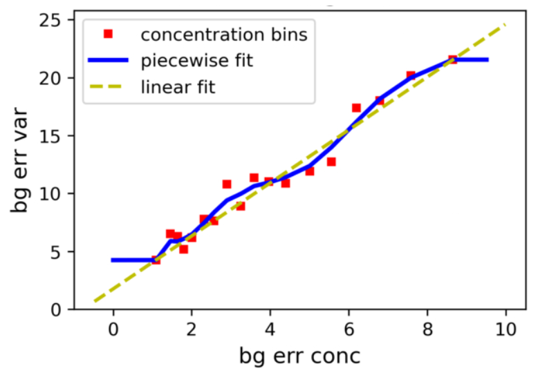
Figure 1 Example of fit functions for background error variances (in (µg m⁻³)²) as function of background state concentrations (in µg m⁻³) of PM_2.5. Red squares: bins (mean values over each concentration bin, from cross-validation at observation stations), Blue solid line: bounded averaged piecewise linear fit used in OAv2. Yellow dashed line: Simple linear fit used in PUF.

To improve the input fields for PM_2.5 error standard deviation w.r.t. these aspects, a simple linear fit of the state-to-variance function has been implemented which is given by the mean slope α_ξ and the offset β_ξ of the concentration bins. This linear state-to-variance relation is applied to the initial- and boundary fields of PM_2.5 concentrations of this case study ξ(x,t) to get case-specific estimates of the related input fields of PM_2.5 concentration error standard deviation σ_ξ(x,t):

$$\begin{array}{}\text{(19)}& {\displaystyle }{\mathit{\sigma }}_{\mathit{\xi }}(\mathit{x},t)=\sqrt{V_{\mathit{\xi }}(\mathit{x},t)}\approx \sqrt{{\mathit{\alpha }}_{\mathit{\xi }}\cdot \mathit{\xi }(\mathit{x},t)+{\mathit{\beta }}_{\mathit{\xi }}}\end{array}$$

Here, PM_2.5 concentrations are calculated as sum over the seven individual prognostic fields of fine aerosol: elemental carbon, primary carbon, organic carbon, nitrate, sulfate, ammonium and crustal material. Figure 1 shows the bounded piecewise and linear fit for state-to-variance relations of PM_2.5 concentrations used in this case study. Eq. (19) only applies to concentration fields like initial- and lateral boundary conditions, because they have the same quantity as the prognostic field.

For point emissions, the linear relation between emissions and concentrations (compare Sect. 2.3) allows the use of the same slope α_E=α_ξ, which also retains the emission-concentration consistency discussed above. However, this does not hold for the offset, for which a conversion depends e.g. on the specific distribution of emissions into different vertical levels. Assuming that the offset is not as dominant as the linear slope, the linear slope with zero offset is used to estimate the correlated emission error standard deviation (compare Sect. 2.3 and Appendix A6.1):

$$\begin{array}{}\text{(20)}& {\displaystyle }{\mathit{\sigma }}_{\mathrm{E}}^{\mathit{\xi }}(\mathit{x},t)=\sqrt{V_{\mathrm{E}}^{\mathit{\xi }}(\mathit{x},t)}\approx \sqrt{{\mathit{\alpha }}_E\cdot E(\mathit{x},t)}\end{array}$$

where E(x,t) are the spatio-temporal fields of PM_2.5 state emissions as sum of the seven aerosol components. Here, the use of the correlated emission error standard deviation as joint input parameter ensures the emission-concentration consistency described above.

In contrast to the OAv2 where this fit is again applied to a 2 month running mean concentration field, it is here applied to the instant concentration field at each location to already include some state-dependency of errors in the input fields.

4 Case Study Application

The PM_2.5 error standard deviation forecast in GEM-MACH is applied to a wildifre smoke episode in a preliminary case study. The purpose of this case study is not to provide a detailed case analysis, but rather to provide an initial proof of concept and exemplary demonstration of potential impacts and benefits of parametric error estimates in an air quality assimilation system compared to the current setup. This section includes the description of the case study and the simulation setup in Sect. 4.1, and the results of error standard deviations and analysis increments in Sect. 4.2 and 4.3, respectively. The results of the parametric experiments presented in this section are calculated with a vertical error correlation length of 6 model layers (approx. 385 m height at the surface over flat terrain). This value was selected from comparison of different vertical error correlation lengths discussed in Appendix D.

4.1 Case Study Description and Model Setup

Starting on 5 June 2023, a set of strong wildfires occurred in central Quebec, in eastern Canada. Despite wildfire sources were located far away from large cities, their smoke plumes were transported southwards reaching the highly populated regions in southern Quebec, Toronto and into northern USA, fumigating New York City within one to two days. Additional figures showing meteorological conditions during the study period are given in Appendix C.

This study focuses on the core phase of the wildfire episode on 6 June 2023 where the main large-scale transport happened, the initial smoke plume reached Montreal and Ottawa, while the wildfires continued at sources much further north (compare Fig. C1). Figure 2 shows the temporal evolution of PM_2.5 surface concentrations simulated by the regional GEM-MACH which serve as background concentrations in the hourly assimilation. The simulation was initialized on 4 June 00:00 UTC with a 24 h forecast spinup. From 5 June 00:00 UTC three subsequent simulations of 12 h each were performed to include updates to the most recent meteorological fields by operational IAU (Incremental Analysis Update)-assimilation and wildfire emissions from CFFEPS. For all results, the simulation is performed for the complete operational regional domain covering north America (denoted as “simulation domain” thereafter), but only part of it shown here focusing on eastern Canada from central Quebec to US border (denoted as “study domain” thereafter).

The PM_2.5 concentration forecast shows several strong plumes related to wildfire hotspots in central Quebec. The largest surface concentrations are induced by the two large wildfire hotspots that are the most north. Besides that, two groups of smaller, but almost similarly strong wildfires can be found in along the Saguenay Fjord in the eastern center, and west of Gouin Reservoir in the western center of study domain. Further south, an old smoke plume that has been emitted the day before induces high PM_2.5 concentrations around the urban areas of Ottawa, Montreal and into the US.

The forecasts of PM_2.5 concentration and error standard deviation are used in the operational OAv2 suite estimating hourly surface analyses w.r.t. all available surface stations in the simulation domain. The setup of the OAv2 suite is equal to the currently operational setup, once using operational error estimates as reference (denoted as “operational experiment” thereafter), and once using parametric error forecasts provided by the GEM-MACH simulation (denoted as “parametric experiment” thereafter). Note that the OAv2 suite only performs hourly surface analyses, with no feedback back into the next forecast. The OAv2 uses an lagged-time ensemble of past forecasts for the same time period to construct spatial error correlations. Spurious error correlations between distant locations are eliminated by applying a Schur product with a compact correlation function based on the Gaspari-Cohn fifth-order spline model (Gaspari and Cohn, 1999). The correlation length-scale of the Gaspari-Cohn model was deterimined by minimizing the analysis error variance evaluated by a cross-validation approach in Ménard and Deshaies-Jacques (2018b).

Using the new parametric error forecast as background error variances in the OAv2 assimilation induces three main differences to the operational formulation of background error variances: Firstly, the operational setup uses a bounded piecewise fit for the state-to-variance relation while the parametric setup uses a fully linear relation (compare Sect. 3.3). Secondly, this relation is applied to mean concentrations over a 2 month time period in the operational setup while being applied to instant concentration forecasts the parametric setup. Thirdly, the calculated error variances are directly used as background error estimates, thus providing purely statistical error estimates to the operational assimilation, while they only serve as input in the parametric error forecast providing highly case-dependent error estimates.

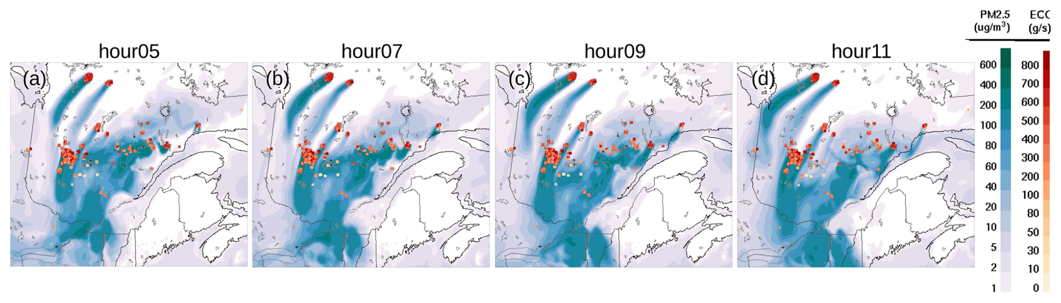
Figure 2 Modeled surface PM_2.5 concentration forecast on 6 June 2023 (blue color code) with wildfire fire locations represented as surface CO emission rates (orange color code) during case study period (hours in UTC).

4.2 Error standard deviation forecasts

Figure 3 shows the surface fields of PM_2.5 error standard deviation (also denoted as “error” thereafter) from the operational experiment and from the new parametric forecast. The parametric fields show significantly higher errors and gradients than the operational experiment, particularly in the regions affected by wildfires. This is because the operational error fields are estimated from long-term statistics and thus cannot account for case-specific uncertainties, particularly from wildfires (Fig. 3a–d). In contrast, the explicit consideration of emission uncertainties in the parametric forecast induces major error sources at the remote wildfire hotspots in central Quebec (Fig. 3e–h). Once emitted, the errors are propagated by advection and vertical diffusion, similar to the dynamics of the state concentrations (compare Sect. 2). Consequently, the extension of the error plumes and their propagation southwards to urban areas is qualitatively similar to the concentration fields (compare Fig. 2).

Nevertheless, there are conceptual differences between the error field from the parametric forecast and the concentration forecast which are of high importance. Firstly, the error forecast does not include modifications due to processes like area emissions, chemical conversions and deposition (compare Sect. 2). Most significantly is the neglection of area emissions in the southern part including the urban areas of Montreal and Toronto. In these areas, the parametric errors are more similar to the operational error fields.

Secondly, the forecasted errors are reduced by the additional correlation term in the diffusion equation (compare Sect. 2.2). This term acts continuously on the error field reducing emission-related errors during their dispersion from sources to other regions. Consequently, the plumes of errors due to uncertain wildfire emissions vanish more quickly than the wildfire plumes in the concentration fields in Fig. 2. It can be seen from Eq. (12) that the strength of the correlation term is determined by the vertical error correlation length. A comparison for different vertical error correlation lengths in Appendix D shows that the impact on error standard deviation forecasts is stronger for shorter vertical error standard deviations.

It is important to note that the qualitative similarity of the error and state concentration forecast fields remains throughout the forecast period only because no analysis is feed back into the subsequent forecast in this simplified case study. In the analysis step, the change of state and error standard deviation due to assimilation of observations differ considerably. While the analysis state is a weighted linear combination between background and observation state, the analysis error standard deviation is always smaller than both, background and observation errors. Thus, the state and error forecasts differ more prominently as soon as any observation is assimilated in the system (see e.g. Voshtani et al., 2022,  for an example).

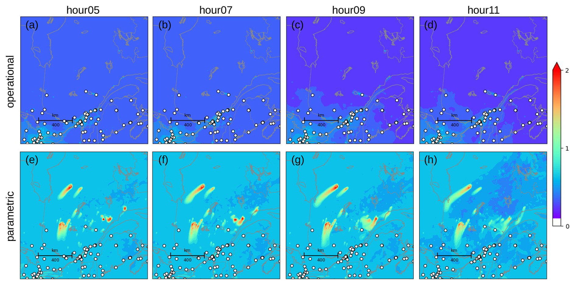
Figure 3 Background error standard deviations fields on 6 June 2023 (logarithmic color code, colorbar labels represent exponent in log ₁₀ (µg m⁻³), hours in UTC) from operational setup (a–d) and parametric forecast with $L_{\mathit{\xi }}^z=\mathrm{6}$ model layers (e–h). Assimilated surface observations are overplotted as white dots.

4.3 Analysis Increments

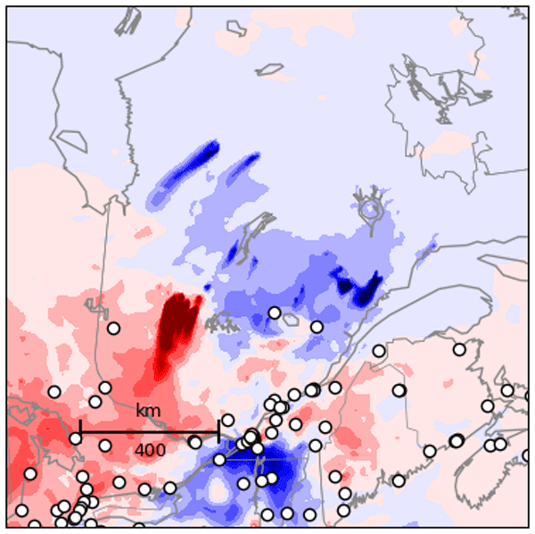
Figure 4 shows analysis increments for surface PM_2.5 from assimilating hourly surface observations into the operational experiment and the new parametric experiment. Generally, analysis increments vary significantly over time in both experiments, especially in the wildfire regions in central Quebec (central and northern part of the study domain) where the observation network is coarse. Note that the no-feedback setup in this study induces that each analysis increment is independent from the previous analyses the hours before, thus opposite corrections of wildfire plumes over time indicate highly variable forecast errors in opposite direction rather than balancing of previous analysis increments.

In the urban areas (southern part of the study domain), the new parametric experiments shows very similar analysis increments compared to the operational experiment w.r.t. both, spatial distribution and strength. A distinct area of strongly negative increments is moving from Ottawa south-eastward across the US border towards Boston and New York City. A comparison to the state forecast of the day before (not shown) indicates an overestimation of old wildfire plume concentrations which is spatio-temporally consistently captured by the urban observation network. The similarity between the two experiments can be attributed to their comparable error standard deviation fields (compare Fig. 3) in combination with good observation coverage in the urban areas leading to low impact of the parametric formulation.

In contrast, the parametric experiment shows considerably large increments in the northern remote areas along the wildfire plumes throughout the simulation period that cannot be found in the operational experiment. The strongly enhanced errors predicted by the parametric forecast along the plumes (compare Fig. 3e–h) induce exceptional spatial spreading of distant observation signals specifically to these locations. Consequently, analysis increments locally exceed values of 80 µg m⁻³ even in the two large northern plumes which are about 400 km away from the nearest observation stations.

It is important to note that the two experiments only differ in their background error standard deviations, not in horizontal error correlation. The spreading of observation signals in the assimilation system is determined by the background error covariance matrix whose off-diagonal covariances are a product of background correlations between the two locations and their background error standard deviations. Thus, the large error standard deviations within the wildfire plumes in the parametric experiment enable significant increments even from weakly correlated observations.

Due to its large error estimates along the wildfire plumes, the parametric formulation induces analysis increments that are explicitly aligned with the forecasted plumes. In the remote wildfire areas with low observation coverage, increments are often attributed commonly to all surrounding plumes within a large region. For example, the two large northern plumes and the plumes close to the Saguenay Fjord are often commonly constraint by the two observations at the Fjord. Nevertheless, the parametric experiment is still able to distinguish between individual plumes if different nearby observations indicate contradicting signals. When the observation constraint is strong enough, even strong opposite increments within a single plume can be found in the parametric experiment. Most prominently, the group of wildfire plumes in the western center of the study area (west of Gouin Reservoir) has strong local increments with opposite signs at 05:00 UTC (Fig. 4e).

Note that the selection of vertical error correlation length also impacts the analysis increments as discussed in Appendix D. However, the comparison shows that the general properties of the parametric experiment described here remain applicable as long as vertical error correlation lengths stays within reasonable ranges.

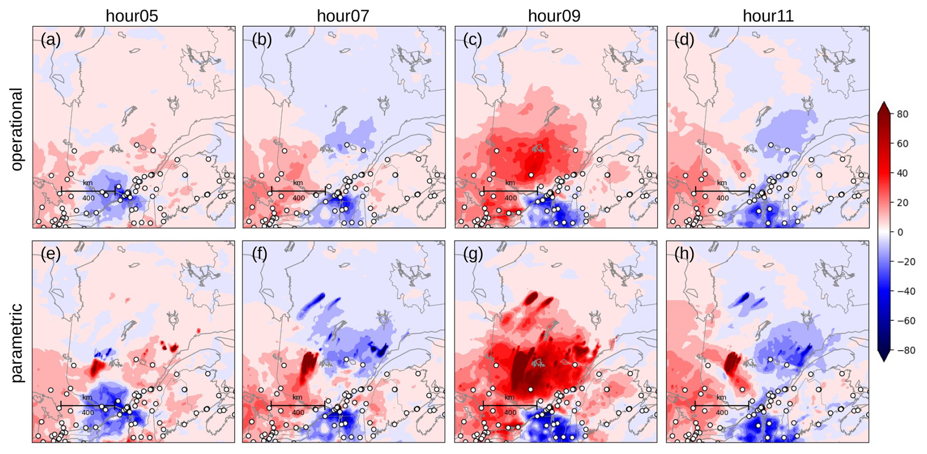
Figure 4 Analysis increments on 6 June 2023 (linear color code, colorbar labels give analysis-background increments in µg m⁻³, hours in UTC) from operational setup (a–d) and parametric forecast with $L_{\mathit{\xi }}^z=\mathrm{6}$  model layers (e–h). Assimilated surface observations are overplotted as white dots.

5 Discussion and Conclusions

This study provides a simple parametric uncertainty forecast (PUF) specifically tailored to the requirements of operational air quality data assimilation under highly uncertain emissions like wildfire smoke events. Operational smoke assimilation systems require fast, yet accurate error estimations which are able to represent the highly case-dependent, large and spatio-temporally variable uncertainties. While ensemble approaches have been demonstrated their suitability to capture such complex case-dependent uncertainties, their high computational costs are a major limitation especially in operational systems. Here, the potential of the PUF is exploited as an alternative approach in which the main error parameters are explicitly handled in the forecast model. This study focuses on (1) the theoretical derivation and investigation of forecast dynamics specific to the requirements of near-surface air quality applications under uncertain emissions, and (2) the setup and implementation of PM_2.5 forecast error standard deviation into the GEM-MACH modeling system.

The first step requires the selection of important processes to be considered in the forecast of error parameters which is especially critical given the operational needs and limitations. The selection of advection, vertical diffusion and point emissions is made upon the principle “as few as possible, as many as necessary” to ensure fast, yet accurate error estimates for near-surface air quality applications. Parametric diffusion and emission processes are considered in a state-of-the-science atmospheric model for the first time in this study. It turned out that error standard deviation is a more suitable parameter than variance because of multiple advantages that range from unit equivalence to simpler forecast equations which increase numerical accuracy and facilitate process-understanding (compare Sect. 2).

Although these two processes are critical for accurate error forecasts in air quality, they are highly sensitive to other error parameters. Is is shown that point emissions only change error parameters if the emissions are considered to be uncertain. Then, the increase of concentration error standard deviation is directly given by the related emission error standard deviation which thus significantly impacts the error forecast, especially for highly uncertain wildfire emissions. The change of error standard deviation or variance due to diffusion is shown to be sensitive to the respective error correlations (compare Appendices B2 and D). In this study, the vertical error correlation length is selected in a rather simple way to retain low computational demands and a decent amount of modifications in the forecast model. More sophisticated formulations will be investigated in future.

In the second step, the implementation into the GEM-MACH modeling system, the simpler forecast equation of error standard deviation becomes also advantageous because it only requires minor modifications in the forecast model (compare Sect. 3). In this study, correlated error variances of point emissions w.r.t. concentration errors are assumed to be proportional to local state emissions. Although this proportionality is consistent with the definitions of initial and boundary conditions (emission-concentration consistency), it is a highly simplified assumption of emission error behavior. This joint quantity consists of the emission error standard deviation and its correlation to the current concentration error which are both difficult to estimate and can be expected to have complex spatio-temporal patterns, particularly for strong case-dependent wildfire emissions. Ideally, each component would be individually estimated from detailed analysis studies which are beyond the scope if this work. Concerning the emission error, each preparation step including detection, quantification and vertical distribution of emissions due to plume rise may have itself complex error sources that would need to be considered. It is demonstrated in Appendix (A6.2) that the emission-concentration correlation is closely related to the temporal correlation of emission errors and potentially also to other dynamical processes modifying the error field, whose estimates are still to be investigated in future. Available studies on aerosol layer and plume height comparisons (e.g. Griffin et al., 2020) will provide a valuable basis for more sophisticated process-based emission uncertainty estimates. The current approach does also not account for uncertainties in emission forecasts of existing fires and their dynamics as well as uncertainties due to potential onset of new fires. Thus, the presented formulation only serves as first simple approach with focus on computational efficiency with large potential for future improvements.

For initial- and boundary conditions of error standard deviation, a simple linear state-to-variance relation is used to ensure emission-concentration consistency between uncertainties originating from uncertain emissions before and within the simulation period. Theoretically, this consistency would also hold in space, i.e. between emission uncertainties inside and outside of the forecast domain, but only if the related state input fields are consistent. In the current regional GEM-MACH, initial conditions are defined case-specific from the previous forecast, while monthly climatologies are used for lateral boundary conditions. Certainly, climatological boundary conditions are expected to have significantly larger uncertainties than case-specific initial conditions, even when – or exactly because – they have smaller concentrations. This inconsistency is not accounted for in the current setup, and thus boundary conditions for error fields are likely to underestimate true uncertainties. However, lateral boundary conditions play a minor role in the high-emission case presented here because state concentrations and their uncertainties are highly dominated by emissions and plume transport within the selected domain (see also Vogel et al., 2026a). Ongoing developments of a global GEM-MACH would enable consistent input fields for state- as well as error fields.

Using these PM_2.5 error standard deviation forecast for assimilation of surface PM_2.5 in an exemplary wildfire case study demonstrates some important properties of the PUF for operational air quality. Firstly, the forecast of PM_2.5 error standard deviation in GEM-MACH shows the suitability of parametric error forecasts in operational air quality systems. The application to wildfire smoke plumes demonstrates its ability to generate highly case-specific and anisotropic error fields at very low computational costs. Moreover, the error forecast results enable explicit investigation of the downstream propagation of errors due to highly uncertain emission sources. Secondly, the large spatio-temporal variability of the PUF-based analysis increments show its ability of case and flow-dependent corrections. For low observation coverage close to remote wildfire hotspots, the large background errors within the plumes enable specific spreading of distant observation information to these uncertain areas.

It is important to note that these significant increments far away from observations are only induced by large forecasted error standard deviations, not exaggerated background error correlations (see Sect. 4.3). In turn, this specific information spearing also means that corrections of remote wildfire plumes are highly determined by a few distant observations, each having significant influence on both, strength and shape on the corrections. This makes the PUF-based assimilation results more sensitive to individual observation information, while making improved use of the sparse observation network in this case study. For increased observation coverage, the PUF error estimates allow for more local corrections with possibly opposite increments within individual plumes, while keeping the consistency within a plume if confirmed by the observations. Thus, even the highly simplified PUF formulation used here enables highly specific and efficient use of the information content provided by sparse observation networks.

Although the error forecast model presented here was developed for wildfire smoke applications, it is generally applicable to other air quality events with highly uncertain emissions. Moreover, the implementation allows for a straight-forward extension to error standard deviation fields of multiple species in the model. This would however require some investigation concerning the validity of selected processes and potential cross-species correlations (see Perrot et al., 2023). Future work will first of all focus on a comprehensive validation of the analysis and its feedback back into the next forecast to enable full PKF assimilation cycling for air quality when it is available in the GEM-MACH model. The general technical implementation of a full assimilation cycling in GEM-MACH is currently a development priority for research as well as operational purposes. In this context, extension of the surface analysis scheme to the full 3D space is required which will also enable comprehensive evaluation of elevated plumes with satellite-based observations. The parametric from of an assimilation cycle also requires the analysis equation for the error parameters that will serve as initial conditions for the next error forecast. This parametric cycling is expected to show more clearly its benefits in terms of improved forecasts as well as understanding of error dynamics throughout multiple forecast-analysis cycles.

Concerning the forecast of error standard deviation of PM_2.5, there are multiple potential improvements. These include for example improved formulations of error parameters like vertical error correlations and emission errors, including their correlation to concentration errors, the consideration of other uncertainties like wind, and the inclusion of other processes like area emissions, chemical conversions or deposition. The latter will be investigated in detail in a follow-up study. Concentration uncertainties due to wind might become particularly important for wildfires because their usual alignment with streamlines might not be applicable during such rapidly developing events. In addition, horizontal diffusion is not considered in this study because the regional operational GEM-MACH configuration does not include horizontal diffusion of the tracer fields. This is based on the assumption that numerical diffusion dominates physical horizontal diffusion in the regional domain. From a theoretical perspective, this assumption would in turn imply that the errors are still reduced by horizontal diffusion, even if the diffusion is caused by numerics rather than an explicit dynamical process. The consideration of related errors would require a considerably different derivation because it purely originates from the specific diffusion scheme in the model rather than the underlying partial differential equations (PDEs). Theoretical studies e.g. by Pannekoucke et al. (2021); Ménard et al. (2021); Gilpin et al. (2025); Gilpin (2026) discuss inaccuracies in parametric error propagation due to discrete dynamics. For simplification, the current formulation only relates to uncertainties in the PDEs and thus implicitly assumes that the discrete numerical schemes are accurate.

Appendix A: Derivation of error dynamics

Numbers in brackets about equal signs indicate equation numbers used in this equation.

A1 Advection-diffusion-emission equation for errors

Let ξ^t(x,t) be the true concentration state of a passive tracer field propagated by an advection-diffusion-emission equation:

$$\begin{array}{}\text{(A1)}& \begin{array}{rl}{\partial }_t{\mathit{\xi }}^{\mathrm{t}}(\mathit{x},t)& =-\mathit{u}(\mathit{x},t)\cdot \mathrm{\nabla }{\mathit{\xi }}^{\mathrm{t}}(\mathit{x},t)\\ & +\mathrm{\nabla }\left(\mathit{\kappa }\right(\mathit{x},t)\cdot \mathrm{\nabla }{\mathit{\xi }}^{\mathrm{t}}(\mathit{x},t\left)\right)+E^{\mathrm{t}}(\mathit{x},t)\end{array}\end{array}$$

with true wind vector field u(x,t), diffusion tensor field κ(x,t) and emission field E^t(x,t).

Assuming an accurate dynamical model with true diffusion coefficient and wind fields, the estimated tracer field ξ(x,t) is propagated by the same advection equation:

$$\begin{array}{}\text{(A2)}& \begin{array}{rl}{\partial }_t\mathit{\xi }(\mathit{x},t)& =-\mathit{u}(\mathit{x},t)\cdot \mathrm{\nabla }\mathit{\xi }(\mathit{x},t)\\ & +\mathrm{\nabla }\left(\mathit{\kappa }\right(\mathit{x},t)\cdot \mathrm{\nabla }\mathit{\xi }(\mathit{x},t\left)\right)+E(\mathit{x},t)\end{array}\end{array}$$

with E(x,t) the estimated emission field in the model.

Further, assuming unbiased random errors for concentrations ϵ_ξ(x,t) and emissions ϵ_E(x,t):

$$\begin{array}{}\text{(A3)}& {\displaystyle }{\mathit{ϵ}}_{\mathit{\xi }}(\mathit{x},t):=& {\displaystyle }\mathit{\xi }(\mathit{x},t)-{\mathit{\xi }}^{\mathrm{t}}(\mathit{x},t)\text{(A4)}& {\displaystyle }{\mathit{ϵ}}_{\mathrm{E}}(\mathit{x},t):=& {\displaystyle }E(\mathit{x},t)-E^{\mathrm{t}}(\mathit{x},t)\end{array}$$

the propagation of concentration error ϵ_ξ(x,t) due to advection-diffusion-emission processes is given as follows:

$$\begin{array}{}\text{(A5)}& \begin{array}{rl}{\partial }_t{\mathit{ϵ}}_{\mathit{\xi }}(\mathit{x},t)\stackrel{\left(\mathrm{A}\mathrm{3}\right)}{=}& {\partial }_t\left({\mathit{\xi }}^{\mathrm{t}}\right(\mathit{x},t)-\mathit{\xi }(\mathit{x},t\left)\right)={\partial }_t{\mathit{\xi }}^{\mathrm{t}}(\mathit{x},t)\\ & -{\partial }_t\mathit{\xi }(\mathit{x},t)\\ \stackrel{(\mathrm{A}\mathrm{1},\mathrm{A}\mathrm{2})}{=}& [-\mathit{u}(\mathit{x},t)\cdot \mathrm{\nabla }{\mathit{\xi }}^{\mathrm{t}}(\mathit{x},t)\\ & +\mathrm{\nabla }\left(\mathit{\kappa }\right(\mathit{x},t)\cdot \mathrm{\nabla }{\mathit{\xi }}^{\mathrm{t}}(\mathit{x},t\left)\right)+E(\mathit{x},t)]\\ & -[-\mathit{u}(\mathit{x},t)\cdot \mathrm{\nabla }\mathit{\xi }(\mathit{x},t)\\ & +\mathrm{\nabla }\left(\mathit{\kappa }\right(\mathit{x},t)\cdot \mathrm{\nabla }\mathit{\xi }(\mathit{x},t\left)\right)+E(\mathit{x},t)]\\ =& -\mathit{u}(\mathit{x},t)\cdot \mathrm{\nabla }\left({\mathit{\xi }}^{\mathrm{t}}\right(\mathit{x},t)-\mathit{\xi }(\mathit{x},t\left)\right)\\ & +\mathrm{\nabla }\left(\mathit{\kappa }\right(\mathit{x},t)\cdot \mathrm{\nabla }\left({\mathit{\xi }}^{\mathrm{t}}(\mathit{x},t)-\mathit{\xi }(\mathit{x},t)\right))\\ & +E^{\mathrm{t}}(\mathit{x},t)-E(\mathit{x},t)\\ \stackrel{\left(\mathrm{A}\mathrm{4}\right)}{=}& -\mathit{u}(\mathit{x},t)\cdot \mathrm{\nabla }{\mathit{ϵ}}_{\mathit{\xi }}(\mathit{x},t)\\ & +\mathrm{\nabla }\left(\mathit{\kappa }\right(\mathit{x},t)\cdot \mathrm{\nabla }{\mathit{ϵ}}_{\mathit{\xi }}(\mathit{x},t\left)\right)+{\mathit{ϵ}}_{\mathrm{E}}(\mathit{x},t)\end{array}\end{array}$$

Thus, the concentration error is propagated with the same linear forecast dynamics as the concentration itself. A more general derivation and discussion of the error propagation equations without emissions can be found in Pannekoucke et al. (2018), their Sect. 3.1.

A2 General propagation of error variance and standard deviation

Given the definitions of error variance and standard deviation in Eq. (3) and Eq. (4), respectively, the general propagation of these two error parameters can be written as follows:

$$\begin{array}{ll}\text{(A6)}& {\displaystyle }{\partial }_t{V}_{\mathit{\xi }}(\mathit{x},t)\stackrel{\left(\mathrm{3}\right)}{=}& {\displaystyle }{\partial }_t\stackrel{\mathrm{‾}}{\left({\mathit{ϵ}}_{\mathit{\xi }}\right(\mathit{x},t){)}^{\mathrm{2}}}=\mathrm{2}\stackrel{\mathrm{‾}}{{\mathit{ϵ}}_{\mathit{\xi }}(\mathit{x},t)\cdot {\partial }_t{\mathit{ϵ}}_{\mathit{\xi }}(\mathit{x},t)}{\displaystyle }{\partial }_t{\mathit{\sigma }}_{\mathit{\xi }}(\mathit{x},t)& {\displaystyle }\stackrel{\left(\mathrm{4}\right)}{=}{\partial }_t\sqrt{V_{\mathit{\xi }}(\mathit{x},t)}={\displaystyle \frac{\mathrm{1}}{\mathrm{2}\sqrt{V_{\mathit{\xi }}(\mathit{x},t)}}}\cdot {\partial }_t{V}_{\mathit{\xi }}(\mathit{x},t)\\ \text{(A7)}& {\displaystyle }& {\displaystyle }\stackrel{\left(\mathrm{A}\mathrm{6}\right)}{=}{\displaystyle \frac{\mathrm{1}}{{\mathit{\sigma }}_{\mathit{\xi }}(\mathit{x},t)}}\cdot \stackrel{\mathrm{‾}}{{\mathit{ϵ}}_{\mathit{\xi }}(\mathit{x},t)\cdot {\partial }_t{\mathit{ϵ}}_{\mathit{\xi }}(\mathit{x},t)}\end{array}$$

A3 3D advection equation for error variance and standard deviation

3D advection equation for forecast error ϵ_ξ(x,t) into directions $\mathit{x}:={\left[x,y,z\right]}^{\mathrm{T}}$:

$$\begin{array}{}\text{(A8)}& .{\partial }_t{\mathit{ϵ}}_{\mathit{\xi }}(\mathit{x},t){|}_{\text{adv}}\stackrel{\left(\mathrm{A}\mathrm{5}\right)}{=}-\mathit{u}(\mathit{x},t)\cdot \mathrm{\nabla }{\mathit{ϵ}}_{\mathit{\xi }}(\mathit{x},t)\end{array}$$

Propagation of forecast error variance V_ξ(x,t) by pure advection:

$$\begin{array}{}\text{(A9)}& \begin{array}{rl}.{\partial }_t{V}_{\mathit{\xi }}(\mathit{x},t){|}_{\text{adv}}& \stackrel{\left(\mathrm{A}\mathrm{6}\right)}{=}\mathrm{2}\stackrel{\mathrm{‾}}{{\mathit{ϵ}}_{\mathit{\xi }}(\mathit{x},t)\cdot .{\partial }_t{\mathit{ϵ}}_{\mathit{\xi }}(\mathit{x},t){|}_{\text{adv}}}\\ & \stackrel{\left(\mathrm{A}\mathrm{8}\right)}{=}-\mathrm{2}\mathit{u}(\mathit{x},t)\cdot \stackrel{\mathrm{‾}}{{\mathit{ϵ}}_{\mathit{\xi }}(\mathit{x},t)\cdot \mathrm{\nabla }{\mathit{ϵ}}_{\mathit{\xi }}(\mathit{x},t)}\end{array}\end{array}$$

Using:

$$\begin{array}{}\text{(A10)}& {\displaystyle }\mathrm{\nabla }{V}_{\mathit{\xi }}(\mathit{x},t):=\mathrm{\nabla }\stackrel{\mathrm{‾}}{\left({\mathit{ϵ}}_{\mathit{\xi }}\right(\mathit{x},t){)}^{\mathrm{2}}}=\mathrm{2}\stackrel{\mathrm{‾}}{{\mathit{ϵ}}_{\mathit{\xi }}(\mathit{x},t)\cdot \mathrm{\nabla }{\mathit{ϵ}}_{\mathit{\xi }}(\mathit{x},t)}\end{array}$$

Gives:

$$\begin{array}{}\text{(A11)}& {\displaystyle }\stackrel{\left(\mathrm{A}\mathrm{9}\right)}{⟹}.{\partial }_t{V}_{\mathit{\xi }}(\mathit{x},t){|}_{\text{adv}}\stackrel{\left(\mathrm{A}\mathrm{10}\right)}{=}{\displaystyle }-\mathit{u}(\mathit{x},t)\cdot \mathrm{\nabla }{V}_{\mathit{\xi }}(\mathit{x},t)\end{array}$$

Similarly, the propagation of forecast error standard deviation σ_ξ(x,t) by pure advection:

$$\begin{array}{}\text{(A12)}& \begin{array}{rl}.{\partial }_t{\mathit{\sigma }}_{\mathit{\xi }}(\mathit{x},t){|}_{\text{adv}}& \stackrel{\left(\mathrm{A}\mathrm{7}\right)}{=}{\displaystyle \frac{\mathrm{1}}{{\mathit{\sigma }}_{\mathit{\xi }}(\mathit{x},t)}}\cdot \stackrel{\mathrm{‾}}{{\mathit{ϵ}}_{\mathit{\xi }}(\mathit{x},t)\cdot .{\partial }_t{\mathit{ϵ}}_{\mathit{\xi }}(\mathit{x},t){|}_{\text{adv}}}\\ & \stackrel{\left(\mathrm{A}\mathrm{8}\right)}{=}-{\displaystyle \frac{\mathrm{1}}{{\mathit{\sigma }}_{\mathit{\xi }}(\mathit{x},t)}}\cdot \mathit{u}(\mathit{x},t)\\ & \cdot \stackrel{\mathrm{‾}}{{\mathit{ϵ}}_{\mathit{\xi }}(\mathit{x},t)\cdot \mathrm{\nabla }{\mathit{ϵ}}_{\mathit{\xi }}(\mathit{x},t)}\end{array}\end{array}$$

Using:

$$\begin{array}{}\text{(A13)}& \begin{array}{rl}\mathrm{\nabla }{\mathit{\sigma }}_{\mathit{\xi }}(\mathit{x},t)& :=\mathrm{\nabla }\sqrt{V_{\mathit{\xi }}(\mathit{x},t)}={\displaystyle \frac{\mathrm{1}}{\mathrm{2}\sqrt{V_{\mathit{\xi }}(\mathit{x},t)}}}\mathrm{\nabla }{V}_{\mathit{\xi }}(\mathit{x},t)\\ & \stackrel{\left(\mathrm{A}\mathrm{10}\right)}{=}\cancel{\mathrm{2}}{\displaystyle \frac{\mathrm{1}}{\cancel{\mathrm{2}}{\mathit{\sigma }}_{\mathit{\xi }}(\mathit{x},t)}}\cdot \stackrel{\mathrm{‾}}{{\mathit{ϵ}}_{\mathit{\xi }}(\mathit{x},t)\cdot \mathrm{\nabla }{\mathit{ϵ}}_{\mathit{\xi }}(\mathit{x},t)}\end{array}\end{array}$$

Gives:

$$\begin{array}{}\text{(A14)}& {\displaystyle }\stackrel{\left(\mathrm{A}\mathrm{12}\right)}{⟹}.{\partial }_t{\mathit{\sigma }}_{\mathit{\xi }}(\mathit{x},t){|}_{\text{adv}}\stackrel{\left(\mathrm{A}\mathrm{13}\right)}{=}{\displaystyle }-\mathit{u}(\mathit{x},t)\cdot \mathrm{\nabla }{\mathit{\sigma }}_{\mathit{\xi }}(\mathit{x},t)\end{array}$$

Note that these propagation equations due to advection were also derived by Pannekoucke et al. (2018), their Sect. 3.2.2.

A4 1D diffusion equation for error variance

1D diffusion equation for random error ϵ_ξ(x,t) into direction z:

$$\begin{array}{}\text{(A15)}& .{\partial }_t{\mathit{ϵ}}_{\mathit{\xi }}(\mathit{x},t){|}_{\text{vdiff}}\stackrel{\left(\mathrm{A}\mathrm{5}\right)}{=}{\partial }_z\left({\mathit{\kappa }}^z\right(\mathit{x},t)\cdot {\partial }_z{\mathit{ϵ}}_{\mathit{\xi }}(\mathit{x},t\left)\right)\end{array}$$

with κ^z(x,t) the vertical diffusion coefficient.

Propagation of forecast error variance V_ξ(x,t) by pure diffusion:

$$\begin{array}{}\text{(A16)}& \begin{array}{rl}.{\partial }_t{V}_{\mathit{\xi }}(\mathit{x},t){|}_{\text{vdiff}}& \stackrel{\left(\mathrm{A}\mathrm{6}\right)}{=}\mathrm{2}\stackrel{\mathrm{‾}}{{\mathit{ϵ}}_{\mathit{\xi }}(\mathit{x},t)\cdot .{\partial }_t{\mathit{ϵ}}_{\mathit{\xi }}(\mathit{x},t){|}_{\text{vdiff}}}\\ & \stackrel{\left(\mathrm{A}\mathrm{15}\right)}{=}\mathrm{2}\stackrel{\mathrm{‾}}{{\mathit{ϵ}}_{\mathit{\xi }}(\mathit{x},t)\cdot {\partial }_z\left({\mathit{\kappa }}^z\right(\mathit{x},t)\cdot {\partial }_z{\mathit{ϵ}}_{\mathit{\xi }}(\mathit{x},t\left)\right)}\\ & =\mathrm{2}{\partial }_z{\mathit{\kappa }}^z(\mathit{x},t)\cdot \stackrel{\mathrm{‾}}{{\mathit{ϵ}}_{\mathit{\xi }}(\mathit{x},t)\cdot {\partial }_z{\mathit{ϵ}}_{\mathit{\xi }}(\mathit{x},t)}\\ & +\mathrm{2}{\mathit{\kappa }}^z(\mathit{x},t)\cdot \stackrel{\mathrm{‾}}{{\mathit{ϵ}}_{\mathit{\xi }}(\mathit{x},t)\cdot {\partial }_z^{\mathrm{2}}{\mathit{ϵ}}_{\mathit{\xi }}(\mathit{x},t)}\end{array}\end{array}$$

Using:

$$\begin{array}{ll}{\displaystyle }{\partial }_z{V}_{\mathit{\xi }}(\mathit{x},t)& {\displaystyle }:={\partial }_z\left[\stackrel{\mathrm{‾}}{\left({\mathit{ϵ}}_{\mathit{\xi }}\right(\mathit{x},t){)}^{\mathrm{2}}}\right]\\ \text{(A17a)}& {\displaystyle }& {\displaystyle }=\mathrm{2}\stackrel{\mathrm{‾}}{{\mathit{ϵ}}_{\mathit{\xi }}(\mathit{x},t)\cdot {\partial }_z{\mathit{ϵ}}_{\mathit{\xi }}(\mathit{x},t)}{\displaystyle }{\partial }_z^{\mathrm{2}}{V}_{\mathit{\xi }}(\mathit{x},t)& {\displaystyle }:={\partial }_z^{\mathrm{2}}\left[\stackrel{\mathrm{‾}}{\left({\mathit{ϵ}}_{\mathit{\xi }}\right(\mathit{x},t){)}^{\mathrm{2}}}\right]\\ {\displaystyle }& {\displaystyle }\stackrel{\left(\mathrm{A}\mathrm{17}\mathrm{a}\right)}{=}\mathrm{2}{\partial }_z\left(\stackrel{\mathrm{‾}}{{\mathit{ϵ}}_{\mathit{\xi }}(\mathit{x},t)\cdot {\partial }_z{\mathit{ϵ}}_{\mathit{\xi }}(\mathit{x},t)}\right)\\ \text{(A17b)}& {\displaystyle }& {\displaystyle }=\mathrm{2}\stackrel{\mathrm{‾}}{\left({\partial }_z{\mathit{ϵ}}_{\mathit{\xi }}\right(\mathit{x},t){)}^{\mathrm{2}}}+\mathrm{2}\stackrel{\mathrm{‾}}{{\mathit{ϵ}}_{\mathit{\xi }}(\mathit{x},t)\cdot {\partial }_z^{\mathrm{2}}{\mathit{ϵ}}_{\mathit{\xi }}(\mathit{x},t)}\end{array}$$

Defining normalized errors ${\stackrel{\mathrm{̃}}{\mathit{ϵ}}}_{\mathit{\xi }}(\mathit{x},t)$:

$$\begin{array}{}\text{(A18)}& {\displaystyle }{\stackrel{\mathrm{̃}}{\mathit{ϵ}}}_{\mathit{\xi }}(\mathit{x},t):={\displaystyle \frac{{\mathit{ϵ}}_{\mathit{\xi }}(\mathit{x},t)}{{\mathit{\sigma }}_{\mathit{\xi }}(\mathit{x},t)}}\end{array}$$

$$\begin{array}{}\text{(A19a)}& {\displaystyle }\text{with:}& {\displaystyle }\stackrel{\mathrm{‾}}{{\left({\stackrel{\mathrm{̃}}{\mathit{ϵ}}}_{\mathit{\xi }}(\mathit{x},t)\right)}^{\mathrm{2}}}=:\mathrm{1}\text{by definition,}\text{(A19b)}& {\displaystyle }\text{and:}& {\displaystyle }\stackrel{\mathrm{‾}}{{\stackrel{\mathrm{̃}}{\mathit{ϵ}}}_{\mathit{\xi }}(\mathit{x},t)\cdot {\partial }_z{\stackrel{\mathrm{̃}}{\mathit{ϵ}}}_{\mathit{\xi }}(\mathit{x},t)}=\mathrm{0}\end{array}$$

which follows directly e.g. from Eqs. (A17a) or (A26a) and the definition of the 1D error correlation length into direction z:

$$\begin{array}{}\text{(A20)}& {\displaystyle }{L}_{\mathit{\xi }}^z(\mathit{x},t):=[\stackrel{\mathrm{‾}}{\left({\partial }_z{\stackrel{\mathrm{̃}}{\mathit{ϵ}}}_{\mathit{\xi }}\right(\mathit{x},t){)}^{\mathrm{2}}}{]}^{-\frac{\mathrm{1}}{\mathrm{2}}}\end{array}$$

Gives:

$$\begin{array}{ll}{\displaystyle }\stackrel{\mathrm{‾}}{\left({\partial }_z{\mathit{ϵ}}_{\mathit{\xi }}\right(\mathit{x},t){)}^{\mathrm{2}}}& {\displaystyle }\stackrel{\left(\mathrm{A}\mathrm{18}\right)}{=}\stackrel{\mathrm{‾}}{\left[{\partial }_z\right({\stackrel{\mathrm{̃}}{\mathit{ϵ}}}_{\mathit{\xi }}(\mathit{x},t)\cdot {\mathit{\sigma }}_{\mathit{\xi }}(\mathit{x},t)){]}^{\mathrm{2}}}\\ {\displaystyle }& {\displaystyle }=\stackrel{\mathrm{‾}}{\left({\stackrel{\mathrm{̃}}{\mathit{ϵ}}}_{\mathit{\xi }}\right(\mathit{x},t)\cdot {\partial }_z{\mathit{\sigma }}_{\mathit{\xi }}(\mathit{x},t)+{\partial }_z{\stackrel{\mathrm{̃}}{\mathit{ϵ}}}_{\mathit{\xi }}(\mathit{x},t)\cdot {\mathit{\sigma }}_{\mathit{\xi }}(\mathit{x},t){)}^{\mathrm{2}}}\\ {\displaystyle }& {\displaystyle }=\stackrel{\mathrm{‾}}{\left({\stackrel{\mathrm{̃}}{\mathit{ϵ}}}_{\mathit{\xi }}\right(\mathit{x},t){)}^{\mathrm{2}}}\cdot \left({\partial }_z{\mathit{\sigma }}_{\mathit{\xi }}\right(\mathit{x},t){)}^{\mathrm{2}}\\ {\displaystyle }& {\displaystyle }+\mathrm{2}\stackrel{\mathrm{‾}}{{\stackrel{\mathrm{̃}}{\mathit{ϵ}}}_{\mathit{\xi }}(\mathit{x},t)\cdot {\partial }_z{\stackrel{\mathrm{̃}}{\mathit{ϵ}}}_{\mathit{\xi }}(\mathit{x},t)}\cdot {\partial }_z{\mathit{\sigma }}_{\mathit{\xi }}(\mathit{x},t)\cdot {\mathit{\sigma }}_{\mathit{\xi }}(\mathit{x},t)\\ {\displaystyle }& {\displaystyle }+\stackrel{\mathrm{‾}}{\left({\partial }_z{\stackrel{\mathrm{̃}}{\mathit{ϵ}}}_{\mathit{\xi }}\right(\mathit{x},t){)}^{\mathrm{2}}}\cdot \left({\mathit{\sigma }}_{\mathit{\xi }}\right(\mathit{x},t){)}^{\mathrm{2}}\\ \text{(A21)}& {\displaystyle }\stackrel{(\mathrm{A}\mathrm{19},\mathrm{A}\mathrm{20})}{=}& {\displaystyle }\left({\partial }_z{\mathit{\sigma }}_{\mathit{\xi }}\right(\mathit{x},t){)}^{\mathrm{2}}+(L_{\mathit{\xi }}^z(\mathit{x},t){)}^{-\mathrm{2}}\cdot V_{\mathit{\xi }}(\mathit{x},t)\end{array}$$

And using:

$$\begin{array}{ll}{\displaystyle }\left({\partial }_z{V}_{\mathit{\xi }}\right(\mathit{x},t){)}^{\mathrm{2}}& {\displaystyle }:=\left[{\partial }_z\right({\mathit{\sigma }}_{\mathit{\xi }}(\mathit{x},t){)}^{\mathrm{2}}{]}^{\mathrm{2}}\\ {\displaystyle }& {\displaystyle }=\left(\mathrm{2}{\mathit{\sigma }}_{\mathit{\xi }}\right(\mathit{x},t)\cdot {\partial }_z{\mathit{\sigma }}_{\mathit{\xi }}(\mathit{x},t){)}^{\mathrm{2}}\\ \text{(A22)}& {\displaystyle }& {\displaystyle }=\mathrm{4}{V}_{\mathit{\xi }}(\mathit{x},t)\cdot \left({\partial }_z{\mathit{\sigma }}_{\mathit{\xi }}\right(\mathit{x},t){)}^{\mathrm{2}}\end{array}$$

Gives:

$$\begin{array}{ll}{\displaystyle }\stackrel{\left(\mathrm{A}\mathrm{17}\mathrm{b}\right)}{⟹}{\partial }_z^{\mathrm{2}}{V}_{\mathit{\xi }}(\mathit{x},t)& {\displaystyle }\stackrel{\left(\mathrm{A}\mathrm{21}\right)}{=}\mathrm{2}\left({\partial }_z{\mathit{\sigma }}_{\mathit{\xi }}\right(\mathit{x},t){)}^{\mathrm{2}}\\ {\displaystyle }& {\displaystyle }+\mathrm{2}\left(L_{\mathit{\xi }}^z\right(\mathit{x},t){)}^{-\mathrm{2}}\cdot V_{\mathit{\xi }}(\mathit{x},t)\\ {\displaystyle }& {\displaystyle }+\mathrm{2}\stackrel{\mathrm{‾}}{{\mathit{ϵ}}_{\mathit{\xi }}(\mathit{x},t)\cdot {\partial }_z^{\mathrm{2}}{\mathit{ϵ}}_{\mathit{\xi }}(\mathit{x},t)}\\ {\displaystyle }\stackrel{\left(\mathrm{A}\mathrm{22}\right)}{=}& {\displaystyle }{\displaystyle \frac{\left({\partial }_z{V}_{\mathit{\xi }}\right(\mathit{x},t){)}^{\mathrm{2}}}{\mathrm{2}{V}_{\mathit{\xi }}(\mathit{x},t)}}+\mathrm{2}\left(L_{\mathit{\xi }}^z\right(\mathit{x},t){)}^{-\mathrm{2}}\\ \text{(A23)}& {\displaystyle }& {\displaystyle }\cdot V_{\mathit{\xi }}(\mathit{x},t)+\mathrm{2}\stackrel{\mathrm{‾}}{{\mathit{ϵ}}_{\mathit{\xi }}(\mathit{x},t)\cdot {\partial }_z^{\mathrm{2}}{\mathit{ϵ}}_{\mathit{\xi }}(\mathit{x},t)}\end{array}$$

Which finally gives the propagation of error variance due to 1D diffusion:

$$\begin{array}{ll}{\displaystyle }\stackrel{\left(\mathrm{A}\mathrm{16}\right)}{⟹}.{\partial }_t{V}_{\mathit{\xi }}(\mathit{x},t){|}_{\text{vdiff}}& {\displaystyle }\stackrel{(\mathrm{A}\mathrm{17}\mathrm{a},\mathrm{A}\mathrm{23})}{=}{\partial }_z{\mathit{\kappa }}^z(\mathit{x},t)\cdot {\partial }_z{V}_{\mathit{\xi }}(\mathit{x},t)\\ {\displaystyle }& {\displaystyle }+{\mathit{\kappa }}^z(\mathit{x},t)\cdot \left[{\partial }_z^{\mathrm{2}}{V}_{\mathit{\xi }}\right(\mathit{x},t)\\ {\displaystyle }& {\displaystyle }-{\displaystyle \frac{\left({\partial }_z{V}_{\mathit{\xi }}\right(\mathit{x},t){)}^{\mathrm{2}}}{\mathrm{2}{V}_{\mathit{\xi }}(\mathit{x},t)}}\\ {\displaystyle }& {\displaystyle }-\mathrm{2}\left(L_{\mathit{\xi }}^z\right(\mathit{x},t){)}^{-\mathrm{2}}\cdot V_{\mathit{\xi }}(\mathit{x},t\left)\right]\\ {\displaystyle }=& {\displaystyle }{\partial }_z\left({\mathit{\kappa }}^z\right(\mathit{x},t)\cdot {\partial }_z{V}_{\mathit{\xi }}(\mathit{x},t\left)\right)\\ {\displaystyle }& {\displaystyle }-{\mathit{\kappa }}^z(\mathit{x},t)\cdot {\displaystyle \frac{\left({\partial }_z{V}_{\mathit{\xi }}\right(\mathit{x},t){)}^{\mathrm{2}}}{\mathrm{2}{V}_{\mathit{\xi }}(\mathit{x},t)}}\\ {\displaystyle }& {\displaystyle }-\mathrm{2}{\mathit{\kappa }}^z(\mathit{x},t)\cdot \left(L_{\mathit{\xi }}^z\right(\mathit{x},t){)}^{-\mathrm{2}}\\ {\displaystyle }& {\displaystyle }\cdot V_{\mathit{\xi }}(\mathit{x},t)\\ {\displaystyle }.{\partial }_t{V}_{\mathit{\xi }}(\mathit{x},t){|}_{\text{vdiff}}=& {\displaystyle }{\partial }_z\left({\mathit{\kappa }}^z\right(\mathit{x},t)\cdot {\partial }_z{V}_{\mathit{\xi }}(\mathit{x},t\left)\right)\\ {\displaystyle }& {\displaystyle }-{\mathit{\kappa }}^z(\mathit{x},t)\cdot V_{\mathit{\xi }}(\mathit{x},t)\\ {\displaystyle }& {\displaystyle }\left[{\left({\displaystyle \frac{{\partial }_z{V}_{\mathit{\xi }}(\mathit{x},t)}{\mathrm{2}{V}_{\mathit{\xi }}(\mathit{x},t)}}\right)}^{\mathrm{2}}\right.\\ \text{(A24)}& {\displaystyle }& {\displaystyle }\left.+\mathrm{2}\left(L_{\mathit{\xi }}^z\right(\mathit{x},t){)}^{-\mathrm{2}}\right]\end{array}$$

Note that Pannekoucke et al. (2018) also derive this propagation equations for error variance due to diffusion, in their Sect. 3.2.3, but using the error correlation tensor instead.

A5 1D diffusion equation for error standard deviation

Propagation of forecast error standard deviation σ_ξ(x,t) by 1D diffusion into direction z:

$$\begin{array}{ll}{\displaystyle }.{\partial }_t{\mathit{\sigma }}_{\mathit{\xi }}(\mathit{x},t){|}_{\text{vdiff}}& {\displaystyle }\stackrel{\left(\mathrm{A}\mathrm{7}\right)}{=}{\displaystyle \frac{\mathrm{1}}{{\mathit{\sigma }}_{\mathit{\xi }}(\mathit{x},t)}}\cdot \stackrel{\mathrm{‾}}{{\mathit{ϵ}}_{\mathit{\xi }}(\mathit{x},t)\cdot .{\partial }_t{\mathit{ϵ}}_{\mathit{\xi }}(\mathit{x},t){|}_{\text{vdiff}}}\\ {\displaystyle }& {\displaystyle }\stackrel{\left(\mathrm{A}\mathrm{15}\right)}{=}{\displaystyle \frac{\mathrm{1}}{{\mathit{\sigma }}_{\mathit{\xi }}(\mathit{x},t)}}\\ {\displaystyle }& {\displaystyle }\cdot \stackrel{\mathrm{‾}}{{\mathit{ϵ}}_{\mathit{\xi }}(\mathit{x},t)\cdot {\partial }_z\left({\mathit{\kappa }}^z\right(\mathit{x},t)\cdot {\partial }_z{\mathit{ϵ}}_{\mathit{\xi }}(\mathit{x},t\left)\right)}\\ {\displaystyle }=& {\displaystyle }{\displaystyle \frac{\mathrm{1}}{{\mathit{\sigma }}_{\mathit{\xi }}(\mathit{x},t)}}\cdot {\partial }_z{\mathit{\kappa }}^z(\mathit{x},t)\cdot \stackrel{\mathrm{‾}}{{\mathit{ϵ}}_{\mathit{\xi }}(\mathit{x},t)\cdot {\partial }_z{\mathit{ϵ}}_{\mathit{\xi }}(\mathit{x},t)}\\ \text{(A25)}& {\displaystyle }& {\displaystyle }+{\displaystyle \frac{\mathrm{1}}{{\mathit{\sigma }}_{\mathit{\xi }}(\mathit{x},t)}}\cdot {\mathit{\kappa }}^z(\mathit{x},t)\cdot \stackrel{\mathrm{‾}}{{\mathit{ϵ}}_{\mathit{\xi }}(\mathit{x},t)\cdot {\partial }_z^{\mathrm{2}}{\mathit{ϵ}}_{\mathit{\xi }}(\mathit{x},t)}\end{array}$$

Using:

$$\begin{array}{ll}{\displaystyle }{\partial }_z{\mathit{\sigma }}_{\mathit{\xi }}(\mathit{x},t)& {\displaystyle }={\displaystyle \frac{\mathrm{1}}{\mathrm{2}{\mathit{\sigma }}_{\mathit{\xi }}(\mathit{x},t)}}\cdot {\partial }_z\left({\mathit{\sigma }}_{\mathit{\xi }}\right(\mathit{x},t){)}^{\mathrm{2}}\\ {\displaystyle }& {\displaystyle }={\displaystyle \frac{\mathrm{1}}{\mathrm{2}{\mathit{\sigma }}_{\mathit{\xi }}(\mathit{x},t)}}{\partial }_z{V}_{\mathit{\xi }}(\mathit{x},t)\\ \text{(A26a)}& {\displaystyle }& {\displaystyle }\stackrel{\left(\mathrm{A}\mathrm{17}\mathrm{a}\right)}{=}{\displaystyle \frac{\mathrm{1}}{{\mathit{\sigma }}_{\mathit{\xi }}(\mathit{x},t)}}\cdot \stackrel{\mathrm{‾}}{{\mathit{ϵ}}_{\mathit{\xi }}(\mathit{x},t)\cdot {\partial }_z{\mathit{ϵ}}_{\mathit{\xi }}(\mathit{x},t)}{\displaystyle }{\partial }_z^{\mathrm{2}}{\mathit{\sigma }}_{\mathit{\xi }}(\mathit{x},t)& {\displaystyle }={\partial }_z\left({\partial }_z{\mathit{\sigma }}_{\mathit{\xi }}\right(\mathit{x},t\left)\right)\\ {\displaystyle }& {\displaystyle }\stackrel{\left(\mathrm{A}\mathrm{26}\mathrm{a}\right)}{=}{\partial }_z\left[{\displaystyle \frac{\mathrm{1}}{{\mathit{\sigma }}_{\mathit{\xi }}(\mathit{x},t)}}\cdot \stackrel{\mathrm{‾}}{{\mathit{ϵ}}_{\mathit{\xi }}(\mathit{x},t)\cdot {\partial }_z{\mathit{ϵ}}_{\mathit{\xi }}(\mathit{x},t)}\right]\\ {\displaystyle }=& {\displaystyle }\left({\partial }_z{\displaystyle \frac{\mathrm{1}}{{\mathit{\sigma }}_{\mathit{\xi }}(\mathit{x},t)}}\right)\cdot \stackrel{\mathrm{‾}}{{\mathit{ϵ}}_{\mathit{\xi }}(\mathit{x},t)\cdot {\partial }_z{\mathit{ϵ}}_{\mathit{\xi }}(\mathit{x},t)}\\ {\displaystyle }& {\displaystyle }+{\displaystyle \frac{\mathrm{1}}{{\mathit{\sigma }}_{\mathit{\xi }}(\mathit{x},t)}}\cdot \stackrel{\mathrm{‾}}{\left({\partial }_z{\mathit{ϵ}}_{\mathit{\xi }}\right(\mathit{x},t){)}^{\mathrm{2}}}\\ {\displaystyle }& {\displaystyle }+{\displaystyle \frac{\mathrm{1}}{{\mathit{\sigma }}_{\mathit{\xi }}(\mathit{x},t)}}\cdot \stackrel{\mathrm{‾}}{{\mathit{ϵ}}_{\mathit{\xi }}(\mathit{x},t)\cdot {\partial }_z^{\mathrm{2}}{\mathit{ϵ}}_{\mathit{\xi }}(\mathit{x},t)}\\ {\displaystyle }=& {\displaystyle }-{\displaystyle \frac{\mathrm{1}}{{\mathit{\sigma }}_{\mathit{\xi }}(\mathit{x},t{)}^{\mathrm{2}}}}\cdot {\partial }_z{\mathit{\sigma }}_{\mathit{\xi }}(\mathit{x},t)\cdot \stackrel{\mathrm{‾}}{{\mathit{ϵ}}_{\mathit{\xi }}(\mathit{x},t)\cdot {\partial }_z{\mathit{ϵ}}_{\mathit{\xi }}(\mathit{x},t)}\\ {\displaystyle }& {\displaystyle }+{\displaystyle \frac{\mathrm{1}}{{\mathit{\sigma }}_{\mathit{\xi }}(\mathit{x},t)}}\cdot \stackrel{\mathrm{‾}}{\left({\partial }_z{\mathit{ϵ}}_{\mathit{\xi }}\right(\mathit{x},t){)}^{\mathrm{2}}}\\ \text{(A26b)}& {\displaystyle }& {\displaystyle }+{\displaystyle \frac{\mathrm{1}}{{\mathit{\sigma }}_{\mathit{\xi }}(\mathit{x},t)}}\cdot \stackrel{\mathrm{‾}}{{\mathit{ϵ}}_{\mathit{\xi }}(\mathit{x},t)\cdot {\partial }_z^{\mathrm{2}}{\mathit{ϵ}}_{\mathit{\xi }}(\mathit{x},t)}\end{array}$$

Gives:

$$\begin{array}{ll}{\displaystyle }\stackrel{\left(\mathrm{A}\mathrm{25}\right)}{⟹}& {\displaystyle }.{\partial }_t{\mathit{\sigma }}_{\mathit{\xi }}(\mathit{x},t){|}_{\text{vdiff}}\stackrel{\left(\mathrm{A}\mathrm{26}\mathrm{b}\right)}{=}{\displaystyle \frac{\mathrm{1}}{{\mathit{\sigma }}_{\mathit{\xi }}(\mathit{x},t)}}\cdot {\partial }_z{\mathit{\kappa }}^z(\mathit{x},t)\\ {\displaystyle }& {\displaystyle }\cdot \stackrel{\mathrm{‾}}{{\mathit{ϵ}}_{\mathit{\xi }}(\mathit{x},t)\cdot {\partial }_z{\mathit{ϵ}}_{\mathit{\xi }}(\mathit{x},t)}\\ {\displaystyle }& {\displaystyle }+{\mathit{\kappa }}^z(\mathit{x},t)\cdot \left[{\partial }_z^{\mathrm{2}}{\mathit{\sigma }}_{\mathit{\xi }}(\mathit{x},t)+{\displaystyle \frac{\mathrm{1}}{{\mathit{\sigma }}_{\mathit{\xi }}(\mathit{x},t{)}^{\mathrm{2}}}}\cdot {\partial }_z{\mathit{\sigma }}_{\mathit{\xi }}(\mathit{x},t)\right.\\ {\displaystyle }& {\displaystyle }\left.\cdot \stackrel{\mathrm{‾}}{{\mathit{ϵ}}_{\mathit{\xi }}(\mathit{x},t)\cdot {\partial }_z{\mathit{ϵ}}_{\mathit{\xi }}(\mathit{x},t)}-{\displaystyle \frac{\mathrm{1}}{{\mathit{\sigma }}_{\mathit{\xi }}(\mathit{x},t)}}\cdot \stackrel{\mathrm{‾}}{\left({\partial }_z{\mathit{ϵ}}_{\mathit{\xi }}\right(\mathit{x},t){)}^{\mathrm{2}}}\right]\\ {\displaystyle }\stackrel{\left(\mathrm{A}\mathrm{26}\mathrm{a}\right)}{=}& {\displaystyle }{\partial }_z{\mathit{\kappa }}^z(\mathit{x},t)\cdot {\partial }_z{\mathit{\sigma }}_{\mathit{\xi }}(\mathit{x},t)+{\mathit{\kappa }}^z(\mathit{x},t){\partial }_z^{\mathrm{2}}{\mathit{\sigma }}_{\mathit{\xi }}(\mathit{x},t)\\ {\displaystyle }& {\displaystyle }+{\mathit{\kappa }}^z(\mathit{x},t)\cdot {\displaystyle \frac{\mathrm{1}}{{\mathit{\sigma }}_{\mathit{\xi }}(\mathit{x},t)}}\left({\partial }_z{\mathit{\sigma }}_{\mathit{\xi }}\right(\mathit{x},t){)}^{\mathrm{2}}\\ {\displaystyle }& {\displaystyle }-{\mathit{\kappa }}^z(\mathit{x},t)\cdot {\displaystyle \frac{\mathrm{1}}{{\mathit{\sigma }}_{\mathit{\xi }}(\mathit{x},t)}}\cdot \stackrel{\mathrm{‾}}{\left({\partial }_z{\mathit{ϵ}}_{\mathit{\xi }}\right(\mathit{x},t){)}^{\mathrm{2}}}\\ {\displaystyle }\stackrel{\left(\mathrm{21}\right)}{=}& {\displaystyle }{\partial }_z{\mathit{\kappa }}^z(\mathit{x},t)\cdot {\partial }_z{\mathit{\sigma }}_{\mathit{\xi }}(\mathit{x},t)+{\mathit{\kappa }}^z(\mathit{x},t)\cdot {\partial }_z^{\mathrm{2}}{\mathit{\sigma }}_{\mathit{\xi }}(\mathit{x},t)\\ {\displaystyle }& {\displaystyle }\cancel{+{\mathit{\kappa }}^z(\mathit{x},t)\cdot {\displaystyle \frac{\mathrm{1}}{{\mathit{\sigma }}_{\mathit{\xi }}(\mathit{x},t)}}\cdot \left({\partial }_z{\mathit{\sigma }}_{\mathit{\xi }}\right(\mathit{x},t){)}^{\mathrm{2}}}\\ {\displaystyle }& {\displaystyle }-{\mathit{\kappa }}^z(\mathit{x},t)\cdot {\displaystyle \frac{\mathrm{1}}{{\mathit{\sigma }}_{\mathit{\xi }}(\mathit{x},t)}}\left[\cancel{\left({\partial }_z{\mathit{\sigma }}_{\mathit{\xi }}\right(\mathit{x},t){)}^{\mathrm{2}}}\right.\\ {\displaystyle }& {\displaystyle }\left.+\left(L_{\mathit{\xi }}^z\right(\mathit{x},t){)}^{-\mathrm{2}}\cdot ({\mathit{\sigma }}_{\mathit{\xi }}(\mathit{x},t){)}^{\mathrm{2}}\right]\\ {\displaystyle }=& {\displaystyle }{\partial }_z{\mathit{\kappa }}^z(\mathit{x},t)\cdot {\partial }_z{\mathit{\sigma }}_{\mathit{\xi }}(\mathit{x},t)+{\mathit{\kappa }}^z(\mathit{x},t)\cdot {\partial }_z^{\mathrm{2}}{\mathit{\sigma }}_{\mathit{\xi }}(\mathit{x},t)\\ {\displaystyle }& {\displaystyle }-{\mathit{\kappa }}^z(\mathit{x},t)\cdot \cancel{{\displaystyle \frac{\mathrm{1}}{{\mathit{\sigma }}_{\mathit{\xi }}(\mathit{x},t)}}}\cdot \left(L_{\mathit{\xi }}^z\right(\mathit{x},t){)}^{-\mathrm{2}}\cdot ({\mathit{\sigma }}_{\mathit{\xi }}(\mathit{x},t){)}^{\cancel{\mathrm{2}}}\\ {\displaystyle }=& {\displaystyle }{\partial }_z\left({\mathit{\kappa }}^z\right(\mathit{x},t)\cdot {\partial }_z{\mathit{\sigma }}_{\mathit{\xi }}(\mathit{x},t\left)\right)\\ \text{(A27)}& {\displaystyle }& {\displaystyle }-{\mathit{\kappa }}^z(\mathit{x},t)\cdot \left(L_{\mathit{\xi }}^z\right(\mathit{x},t){)}^{-\mathrm{2}}\cdot {\mathit{\sigma }}_{\mathit{\xi }}(\mathit{x},t)\end{array}$$

A6 Point emission equation for error variance and standard deviation

The change of state concentrations due to point emissions (= locally added emission amount per timestep and gridbox) of each species is given by:

$$\begin{array}{}\text{(A28)}& {\displaystyle }.{\partial }_t\mathit{\xi }(\mathit{x},t){|}_{\text{p.emis}}\stackrel{\left(\mathrm{1}\right)}{=}E(\mathit{x},t)\end{array}$$

Then the error due to uncertainties in the prescribed emission field E(x,t) is given by its deviation from the true emission field E^t(x,t):

$$\begin{array}{}\text{(A29)}& \begin{array}{rl}.{\partial }_t{\mathit{ϵ}}_{\mathit{\xi }}(\mathit{x},t){|}_{\text{p.emis}}& \stackrel{\left(\mathrm{1}\right)}{=}{\partial }_t\left[\mathit{\xi }\right(\mathit{x},t)-{\mathit{\xi }}^{\mathrm{t}}(\mathit{x},t){]}_{\text{p.emis}}\\ & =.{\partial }_t\mathit{\xi }(\mathit{x},t){|}_{\text{p.emis}}-.{\partial }_t{\mathit{\xi }}^{\mathrm{t}}(\mathit{x},t){|}_{\text{p.emis}}\\ & \stackrel{\left(\mathrm{A}\mathrm{28}\right)}{=}E(\mathit{x},t)-E^{\mathrm{t}}(\mathit{x},t):={\mathit{ϵ}}_{\mathrm{E}}(\mathit{x},t)\end{array}\end{array}$$

with ϵ_E(x,t) the error in emission field of that species.

A6.1 General derivation

The change of concentration error variance due to uncertain emissions becomes:

$$\begin{array}{}\text{(A30)}& \begin{array}{rl}.{\partial }_t{V}_{\mathit{\xi }}(\mathit{x},t){|}_{\text{adv}}& \stackrel{\left(\mathrm{2}\right)}{=}\mathrm{2}\stackrel{\mathrm{‾}}{{\mathit{ϵ}}_{\mathit{\xi }}(\mathit{x},t)\cdot .{\partial }_t{\mathit{ϵ}}_{\mathit{\xi }}(\mathit{x},t){|}_{\text{adv}}}\\ & \stackrel{\left(\mathrm{A}\mathrm{28}\right)}{=}\mathrm{2}\stackrel{\mathrm{‾}}{{\mathit{ϵ}}_{\mathit{\xi }}(\mathit{x},t)\cdot {\mathit{ϵ}}_{\mathrm{E}}(\mathit{x},t)}\end{array}\end{array}$$

Defining normalized errors of concentration and emissions:

$$\begin{array}{}\text{(A31a)}& {\displaystyle }{\stackrel{\mathrm{̃}}{\mathit{ϵ}}}_{\mathit{\xi }}(\mathit{x},t):={\displaystyle \frac{{\mathit{ϵ}}_{\mathit{\xi }}(\mathit{x},t)}{{\mathit{\sigma }}_{\mathit{\xi }}(\mathit{x},t)}}\text{(A31b)}& {\displaystyle }{\stackrel{\mathrm{̃}}{\mathit{ϵ}}}_{\mathrm{E}}(\mathit{x},t):={\displaystyle \frac{{\mathit{ϵ}}_{\mathrm{E}}(\mathit{x},t)}{{\mathit{\sigma }}_{\mathrm{E}}(\mathit{x},t)}}\end{array}$$

and the local error correlation between concentrations and emissions:

$$\begin{array}{}\text{(A32)}& {\displaystyle }{\mathit{\rho }}_{\mathrm{E},\mathit{\xi }}(\mathit{x},t):=\stackrel{\mathrm{‾}}{{\stackrel{\mathrm{̃}}{\mathit{ϵ}}}_{\mathit{\xi }}(\mathit{x},t)\cdot {\stackrel{\mathrm{̃}}{\mathit{ϵ}}}_{\mathrm{E}}(\mathit{x},t)}\end{array}$$

Gives:

$$\begin{array}{}\text{(A33)}& \begin{array}{rl}\stackrel{\left(\mathrm{A}\mathrm{30}\right)}{⟹}.{\partial }_t{V}_{\mathit{\xi }}(\mathit{x},t){|}_{\text{p.emis}}& \stackrel{\left(\mathrm{A}\mathrm{31}\right)}{=}\mathrm{2}{\mathit{\sigma }}_{\mathit{\xi }}(\mathit{x},t)\cdot {\mathit{\sigma }}_{\mathrm{E}}(\mathit{x},t)\\ & \cdot \stackrel{\mathrm{‾}}{{\stackrel{\mathrm{̃}}{\mathit{ϵ}}}_{\mathit{\xi }}(\mathit{x},t)\cdot {\stackrel{\mathrm{̃}}{\mathit{ϵ}}}_{\mathrm{E}}(\mathit{x},t)}\\ & \stackrel{\left(\mathrm{A}\mathrm{31}\right)}{=}\mathrm{2}{\mathit{\sigma }}_{\mathit{\xi }}(\mathit{x},t)\\ & \cdot {\mathit{\sigma }}_{\mathrm{E}}(\mathit{x},t)\cdot {\mathit{\rho }}_{\mathrm{E},\mathit{\xi }}(\mathit{x},t)\end{array}\end{array}$$

Similarly, the change of concentration error standard deviation due to uncertain emissions is given by:

$$\begin{array}{ll}{\displaystyle }.{\partial }_t{\mathit{\sigma }}_{\mathit{\xi }}(\mathit{x},t){|}_{\text{p.emis}}& {\displaystyle }\stackrel{\left(\mathrm{A}\mathrm{7}\right)}{=}{\displaystyle \frac{\mathrm{1}}{{\mathit{\sigma }}_{\mathit{\xi }}(\mathit{x},t)}}\cdot \stackrel{\mathrm{‾}}{{\mathit{ϵ}}_{\mathit{\xi }}(\mathit{x},t)\cdot .{\partial }_t{\mathit{ϵ}}_{\mathit{\xi }}(\mathit{x},t){|}_{\text{p.emis}}}\\ {\displaystyle }& {\displaystyle }\stackrel{\left(\mathrm{A}\mathrm{29}\right)}{=}{\displaystyle \frac{\mathrm{1}}{{\mathit{\sigma }}_{\mathit{\xi }}(\mathit{x},t)}}\cdot \stackrel{\mathrm{‾}}{{\mathit{ϵ}}_{\mathit{\xi }}(\mathit{x},t)\cdot {\mathit{ϵ}}_{\mathrm{E}}(\mathit{x},t)}\\ {\displaystyle }& {\displaystyle }\stackrel{\left(\mathrm{A}\mathrm{31}\right)}{=}{\mathit{\sigma }}_{\mathrm{E}}(\mathit{x},t)\cdot \stackrel{\mathrm{‾}}{{\stackrel{\mathrm{̃}}{\mathit{ϵ}}}_{\mathit{\xi }}(\mathit{x},t)\cdot {\stackrel{\mathrm{̃}}{\mathit{ϵ}}}_{\mathrm{E}}(\mathit{x},t)}\\ \text{(A34)}& {\displaystyle }& {\displaystyle }\stackrel{\left(\mathrm{A}\mathrm{32}\right)}{=}{\mathit{\sigma }}_{\mathrm{E}}(\mathit{x},t)\cdot {\mathit{\rho }}_{\mathrm{E},\mathit{\xi }}(\mathit{x},t)\end{array}$$

Since the emission error standard deviation σ_E(x,t) and its correlation to concentration errors ${\mathit{\rho }}_{\mathrm{E},\mathit{\xi }}(\mathit{x},t)$ are both unknown external parameters, they are jointly treated as correlated emission error standard deviation w.r.t. the current concentration error in the following:

$$\begin{array}{}\text{(A35)}& {\displaystyle }{\mathit{\sigma }}_{\mathrm{E}}^{\mathit{\xi }}(\mathit{x},t):={\mathit{\sigma }}_{\mathrm{E}}(\mathit{x},t)\cdot {\mathit{\rho }}_{\mathrm{E},\mathit{\xi }}(\mathit{x},t)\end{array}$$

For a discrete timestep Δt, the concentration error standard deviation increases linearly with the correlated emission error standard deviation:

$$\begin{array}{}\text{(A36)}& {\displaystyle }.{\mathit{\sigma }}_{\mathit{\xi }}(\mathit{x},t){|}_{\text{p.emis}}\stackrel{(\mathrm{A}\mathrm{34},\mathrm{A}\mathrm{32})}{=}{\mathit{\sigma }}_{\mathit{\xi }}(\mathit{x},t_{\mathrm{0}})+{\mathit{\sigma }}_{\mathrm{E}}^{\mathit{\xi }}(\mathit{x},t)\cdot \mathrm{\Delta }t\end{array}$$

with σ_ξ(x,t₀) the concentration error standard deviation at the previous timestep $t_{\mathrm{0}}=t-\mathrm{\Delta }t$.

For comparison, the prognostic equation for concentration error variance in Eq. (A33) includes the concentration error standard deviation on the right-hand-side, which results in a quadratic increase over time:

$$\begin{array}{ll}{\displaystyle }.V_{\mathit{\xi }}(\mathit{x},t){|}_{\text{p.emis}}& {\displaystyle }:={\left[{\mathit{\sigma }}_{\mathit{\xi }}(\mathit{x},t){|}_{\text{p.emis}}\right]}^{\mathrm{2}}\\ {\displaystyle }& {\displaystyle }\stackrel{\left(\mathrm{A}\mathrm{36}\right)}{=}\left[{\mathit{\sigma }}_{\mathit{\xi }}\right(\mathit{x},t_{\mathrm{0}})+{\mathit{\sigma }}_{\mathrm{E}}^{\mathit{\xi }}(\mathit{x},t)\cdot \mathrm{\Delta }t{]}^{\mathrm{2}}\\ {\displaystyle }& {\displaystyle }=V_{\mathit{\xi }}(\mathit{x},t_{\mathrm{0}})+\mathrm{2}{\mathit{\sigma }}_{\mathit{\xi }}(\mathit{x},t_{\mathrm{0}})\cdot {\mathit{\sigma }}_{\mathrm{E}}^{\mathit{\xi }}(\mathit{x},t)\cdot \mathrm{\Delta }t\\ \text{(A37)}& {\displaystyle }& {\displaystyle }+V_{\mathrm{E}}^{\mathit{\xi }}(\mathit{x},t)\cdot [\mathrm{\Delta }t{]}^{\mathrm{2}}\end{array}$$

with V_ξ(x,t₀) the previous concentration error variance.

A6.2 Connection to temporal correlation of emission errors

In the following, the connection of the emission-concentration error correlation ${\mathit{\rho }}_{\mathrm{E},\mathit{\xi }}(\mathit{x},t)$ to the temporal correlation of the emission error ${\mathit{\tau }}_{{\mathit{ϵ}}_{\mathrm{E}}}\left(t\right)$ is demonstrated in a simplified formulation for ${\mathit{\tau }}_{{\mathit{ϵ}}_{\mathrm{E}}}\left(t\right)<\mathrm{\Delta }t$ the model timestep. In this case, the concentration error at time t can be decomposed into its contributions from the emission error ϵ_E(x,t) over the correlated time [t₀,t] and from the prior concentration error ϵ_ξ(x,t₀):

$$\begin{array}{}\text{(A38)}& {\displaystyle }{\mathit{ϵ}}_{\mathit{\xi }}(\mathit{x},t)\stackrel{\left(\mathrm{A}\mathrm{29}\right)}{=}{\mathit{ϵ}}_{\mathit{\xi }}(\mathit{x},t_{\mathrm{0}})+{\mathit{ϵ}}_{\mathrm{E}}(\mathit{x},t)\cdot {\mathit{\tau }}_{{\mathit{ϵ}}_{\mathrm{E}}}\left(t\right)\end{array}$$

with $t_{\mathrm{0}}=t-{\mathit{\tau }}_{{\mathit{ϵ}}_{\mathrm{E}}}\left(t\right)$.

In terms of normalized errors:

$$\begin{array}{ll}{\displaystyle }\stackrel{\left(\mathrm{A}\mathrm{38}\right)}{⟹}{\stackrel{\mathrm{̃}}{\mathit{ϵ}}}_{\mathit{\xi }}(\mathit{x},t)& {\displaystyle }\stackrel{\left(\mathrm{A}\mathrm{31}\right)}{=}{\displaystyle \frac{{\mathit{\sigma }}_{\mathit{\xi }}(\mathit{x},t_{\mathrm{0}})}{{\mathit{\sigma }}_{\mathit{\xi }}(\mathit{x},t)}}\cdot {\stackrel{\mathrm{̃}}{\mathit{ϵ}}}_{\mathit{\xi }}(\mathit{x},t_{\mathrm{0}})\\ \text{(A39)}& {\displaystyle }& {\displaystyle }+{\displaystyle \frac{{\mathit{\sigma }}_{\mathrm{E}}(\mathit{x},t)}{{\mathit{\sigma }}_{\mathit{\xi }}(\mathit{x},t)}}\cdot {\stackrel{\mathrm{̃}}{\mathit{ϵ}}}_{\mathrm{E}}(\mathit{x},t)\cdot {\mathit{\tau }}_{{\mathit{ϵ}}_{\mathrm{E}}}\left(t\right)\end{array}$$

With this, the correlation between emission and concentration errors becomes:

$$\begin{array}{ll}{\displaystyle }{\mathit{\rho }}_{\mathrm{E},\mathit{\xi }}(\mathit{x},t)& {\displaystyle }:=\stackrel{\mathrm{‾}}{{\stackrel{\mathrm{̃}}{\mathit{ϵ}}}_{\mathit{\xi }}(\mathit{x},t)\cdot {\stackrel{\mathrm{̃}}{\mathit{ϵ}}}_{\mathrm{E}}(\mathit{x},t)}\\ {\displaystyle }& {\displaystyle }\stackrel{\left(\mathrm{A}\mathrm{39}\right)}{=}{\displaystyle \frac{{\mathit{\sigma }}_{\mathit{\xi }}(\mathit{x},t_{\mathrm{0}})}{{\mathit{\sigma }}_{\mathit{\xi }}(\mathit{x},t)}}\cdot \stackrel{\mathrm{‾}}{{\stackrel{\mathrm{̃}}{\mathit{ϵ}}}_{\mathit{\xi }}(\mathit{x},t_{\mathrm{0}})\cdot {\stackrel{\mathrm{̃}}{\mathit{ϵ}}}_{\mathrm{E}}(\mathit{x},t)}\\ \text{(A40)}& {\displaystyle }& {\displaystyle }+{\displaystyle \frac{{\mathit{\sigma }}_{\mathrm{E}}(\mathit{x},t)}{{\mathit{\sigma }}_{\mathit{\xi }}(\mathit{x},t)}}\cdot \stackrel{\mathrm{‾}}{{\stackrel{\mathrm{̃}}{\mathit{ϵ}}}_{\mathrm{E}}(\mathit{x},t{)}^{\mathrm{2}}}\cdot {\mathit{\tau }}_{{\mathit{ϵ}}_{\mathrm{E}}}\left(t\right)\end{array}$$

Since $t_{\mathrm{0}}=t-{\mathit{\tau }}_{{\mathit{ϵ}}_{\mathrm{E}}}\left(t\right)$, the prior concentration error ϵ_ξ(x,t₀) is uncorrelated to the current emission error ϵ_E(x,t):

$$\begin{array}{}\text{(A41)}& {\displaystyle }\stackrel{\mathrm{‾}}{{\stackrel{\mathrm{̃}}{\mathit{ϵ}}}_{\mathit{\xi }}(\mathit{x},t_{\mathrm{0}})\cdot {\stackrel{\mathrm{̃}}{\mathit{ϵ}}}_{\mathrm{E}}(\mathit{x},t)}\approx \mathrm{0}\end{array}$$

And using the unit property of normalized errors $\stackrel{\mathrm{‾}}{{\stackrel{\mathrm{̃}}{\mathit{ϵ}}}_{\mathrm{E}}(\mathit{x},t{)}^{\mathrm{2}}}=\mathrm{1}$ gives the approximation:

$$\begin{array}{}\text{(A42)}& {\displaystyle }\stackrel{\left(\mathrm{A}\mathrm{40}\right)}{⟹}{\mathit{\rho }}_{\mathrm{E},\mathit{\xi }}(\mathit{x},t)\stackrel{\left(\mathrm{A}\mathrm{41}\right)}{\approx }{\displaystyle \frac{{\mathit{\sigma }}_{\mathrm{E}}(\mathit{x},t)}{{\mathit{\sigma }}_{\mathit{\xi }}(\mathit{x},t)}}\cdot {\mathit{\tau }}_{{\mathit{ϵ}}_{\mathrm{E}}}\left(t\right)\forall {\mathit{\tau }}_{{\mathit{ϵ}}_{\mathrm{E}}}\left(t\right)<\mathrm{\Delta }t\end{array}$$

which disentangles emission- and concentration errors. Consequently, the emission-concentration correlation becomes proportional to the relative contribution of the emission error from the correlated time to the overall concentration error and increases linearly with the correlation timescale.

This formulation can also be generalized to any timescale ${\mathit{\tau }}_{{\mathit{ϵ}}_{\mathrm{E}}}\left(t\right)>\mathrm{\Delta }t$ by taking into account the other model processes which modify the effective correlation timescale at each timestep. For example, strong advection or diffusion modifying the prior concentration error ${\stackrel{\mathrm{̃}}{\mathit{ϵ}}}_{\mathit{\xi }}(\mathit{x},t_{\mathrm{0}})$ can quickly disentangle it from the current emission error on timescales below ${\mathit{\tau }}_{{\mathit{ϵ}}_{\mathrm{E}}}\left(t\right)$. In this case, Eq. (A41) may still hold for ${\mathit{\tau }}_{{\mathit{ϵ}}_{\mathrm{E}}}\left(t\right)>\mathrm{\Delta }t$.

Appendix B: Idealized experiments for 1D diffusion

B1 Comparison of variance- and standard deviation-form

Figure B1 visualizes the individual terms contributing to the change of error variance and standard deviation due to diffusion in an idealized 1D experiment. Starting from an artificial background variance field (Fig. B1a), a single observation is assimilated at gridpoint 34. Afterwards strong diffusion was considered as forecast step to clearly show the impact of the individual terms for each formulation (Fig. B1b, c). For both formulations, the smoothing effect of the standard diffusion term (term 1) and the overall reducing effect of the correlation term (term 2) are clearly visible (compare Sect. 2.2). However, the variance form has an additional term (gradient term, term 3) which reduces error variance at strong spatial gradients (compare Eq. 11). Because the two formulations are mathematically identical, the first two terms are locally larger in the variance form compared to the standard deviation form in which the impact of the gradient term (term 3) is implicitly accounted for in the other two terms. Consequently, the strength and shape of the first two terms differ between the two formulations.

In terms of interpretability, the standard deviation form shows more clearly the increased reduction by the correlation term (term 2) at locations with reduced error correlations around the observation (compare Eq. 12). A comparison of the net residual of the parametric formulations to the full Kalman Filter shows that the standard deviation form is more accurate which can be attributed to additional numerical uncertainties in the gradient term of the variance form. For a more detailed description of the remaining residuals see Appendix B2.

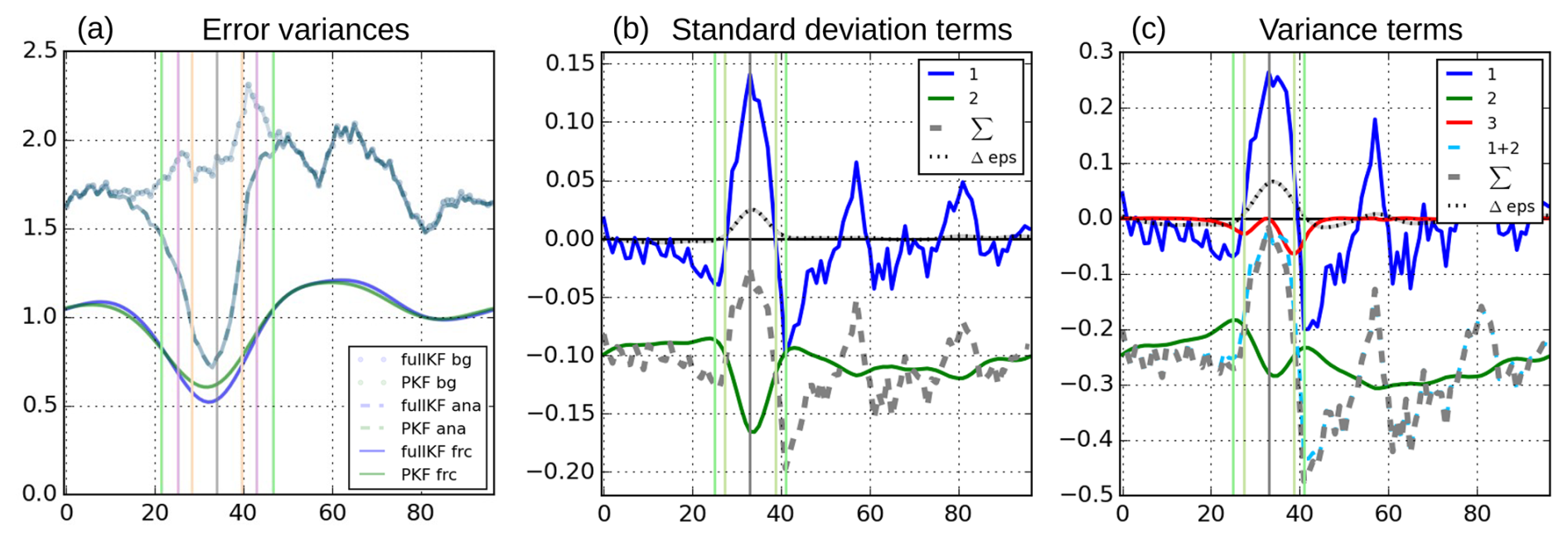
Figure B1 Comparison of individual terms (solid colored lines) in idealized 1D experiment for diffusion calculated (b) from the variance form in Eq. (11) and (c) from the standard deviation form in Eq. (12), respectively, from the first diffusion timestep. Dashed lines indicate the sum over terms 1+2 (light blue) and all terms (gray), respectively. The residual difference to the full KF is given as grey-black dotted line. Vertical lines indicate the observation location (gray), and related error correlation lengths for background (pink), analysis before diffusion (orange), forecast before current diffusion timestep (light green), and after diffusion (green). Note the different units of the vertical axis referring to the change of error variance (b) and standard deviation (c), respectively. Panel (a): variance fields of background (dotted), analysis (dashed) and diffusion forecast (solid) for the full KF (blue) and PKF using the standard deviation form (green), respectively.

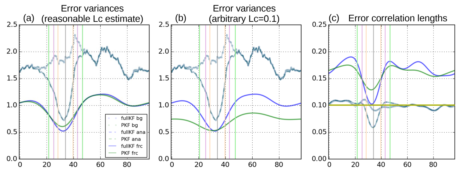
Figure B2 Comparison of idealized 1D experiment for diffusion for different correlation lengths: (a) from reasonable estimate (PKF forecast in (c), same as Fig. B1a), (b) from arbitrarily definition of 0.1=10 gridpoints (mean background in (c)). Plotting convention as in Fig. B1). Panel (c): error correlation length fields of background (dotted), analysis (dashed) and diffusion forecast (solid) for the full KF (blue), reasonable PKF estimate (green) and arbitrary definition (dark yellow), respectively.

B2 Importance of correlation length

The same idealized 1D experiment described in Appendix B1 is used to demonstrate the influence of defined error correlation length on the resulting forecast error variance which has been calculated from the prognostic equation of error standard deviation due to diffusion in Eq. (12). When the parametric forecast error variance after diffusion is calculated with a reasonable estimate of error correlation length in Fig. B2a, it remains accurate compared to the full KF error variance field even for strong diffusion. In this example, this reasonable estimate was achieved by a leading order PUF forecast of error correlation length due to diffusion (e.g. Pannekoucke et al., 2016, their Eq. 24) shown in Fig. B2c.

In contrast, setting the error correlation length to a significantly lower value, the forecast error variance in Fig. B2b is considerably underestimated after strong diffusion. In this example, an arbitrary constant error correlation length of 0.1 (equivalent to 10 gridpoints) was used throughout the whole diffusion process which represents the mean background error correlation length and thus underestimates the final correlation by about 40 % (Fig. B2c). This underestimated correlation results in an overestimation of the reduction of error variance due to diffusion (compare Eq. 12) and thus in an underestimation of the final forecast error variance of about 25 % for most locations (Fig. B2b).

Note that the accurate estimate of forecast error variance at the observation location results only because the true forecast error correlation length happens to be 0.1 in this example (Fig. B2c). Thus, the fact that the arbitrary estimate in Fig. B2b is more accurate around the observation location than the approximative correlation forecast in Fig. B2a is purely by chance and does not have any conceptual reason.

Appendix C: Maps of meteorological conditions for real case experiment

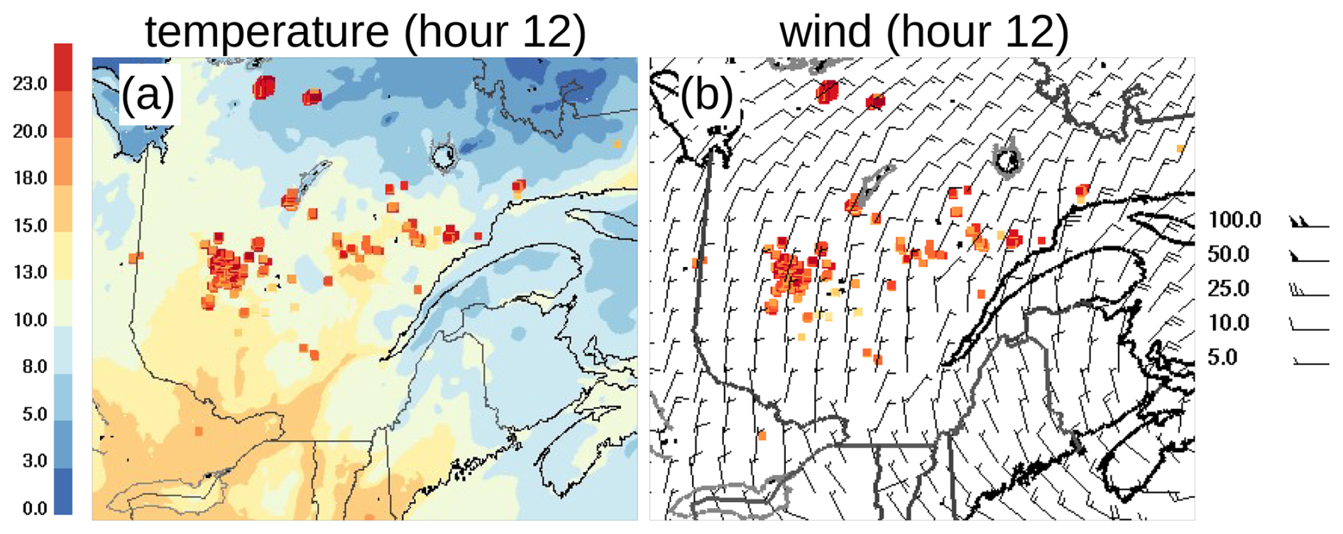
Figure C1 Modeled meteorological conditions 6 June 2023 12:00 UTC: (a) surface temperature in degree Celsius (blue-red color code) and (b) near surface wind speed and direction (wind barbs) with wildfire fire locations represented as surface CO emission rates (orange color code in Fig. 2).

Appendix D: Real case experiments with different vertical error correlation lengths

Because diffusion is constantly acting on a plume since its emission, the impact of the vertical error correlation length is accumulating over time (compare Sect. 2.2). Consequently, the estimated error correlation length has an increasing impact on forecasted error standard deviation far away from sources which can be seen from a comparison in Fig. D1.

A small vertical error correlation length – here $L_{\mathit{\xi }}^z=\mathrm{4}$ vertical model layers (approx. 210 m height at the surface over flat terrain) – induces strong decay of error standard deviations over time which here results in significantly shorter wildfire “uncertainty-plumes” in the forecast of error standard deviation (Fig. D1a–d). For increasing vertical error correlation length – here $L_{\mathit{\xi }}^z$=8 or 10 vertical model layers (approx. 600 m or 865 m height) – the wildfire uncertainty-plumes lengthen and converge to the shape of the wildfire concentration plumes (Fig. D1i–p, compare with Fig. 2) which means that the reduction term in the error diffusion equation Eq. (12) becomes neglectable. Thus, the impact on the error standard deviation forecast is stronger for shorter vertical error standard deviations. The comparison indicates that $L_{\mathit{\xi }}^z=\mathrm{6}$ vertical model layers (approx. 385 m height) appears to be a medium vertical error correlation length which balances a reasonable extension of the uncertainty-plumes with a significant reduction compared to concentration-plumes (Fig. D1e–h) and is therefore selected to be discussed more detailed in Sect. 4. The resulting hourly analysis increments in Fig. D2 are also impacted by the selected vertical error correlation length. In the urban areas, the combination of smaller error standard deviations and more dense observations make the increments generally less influenced by the parametric error fields and therefore less dependent on the vertical error correlation length. In contrast, more significant differences can be found in the sparsely observed regions in the north, where the different lengths of the strong wildfire uncertainty-plumes directly transfer to the spatial patterns of analysis increments. Consequently, the spatial extend of strong analysis increments increases with increasing vertical error correlation length, even if observations induce opposite signs of increments within the same plume (e.g. in the western center of the study area west of Gouin Reservoir at 07:00 UTC).

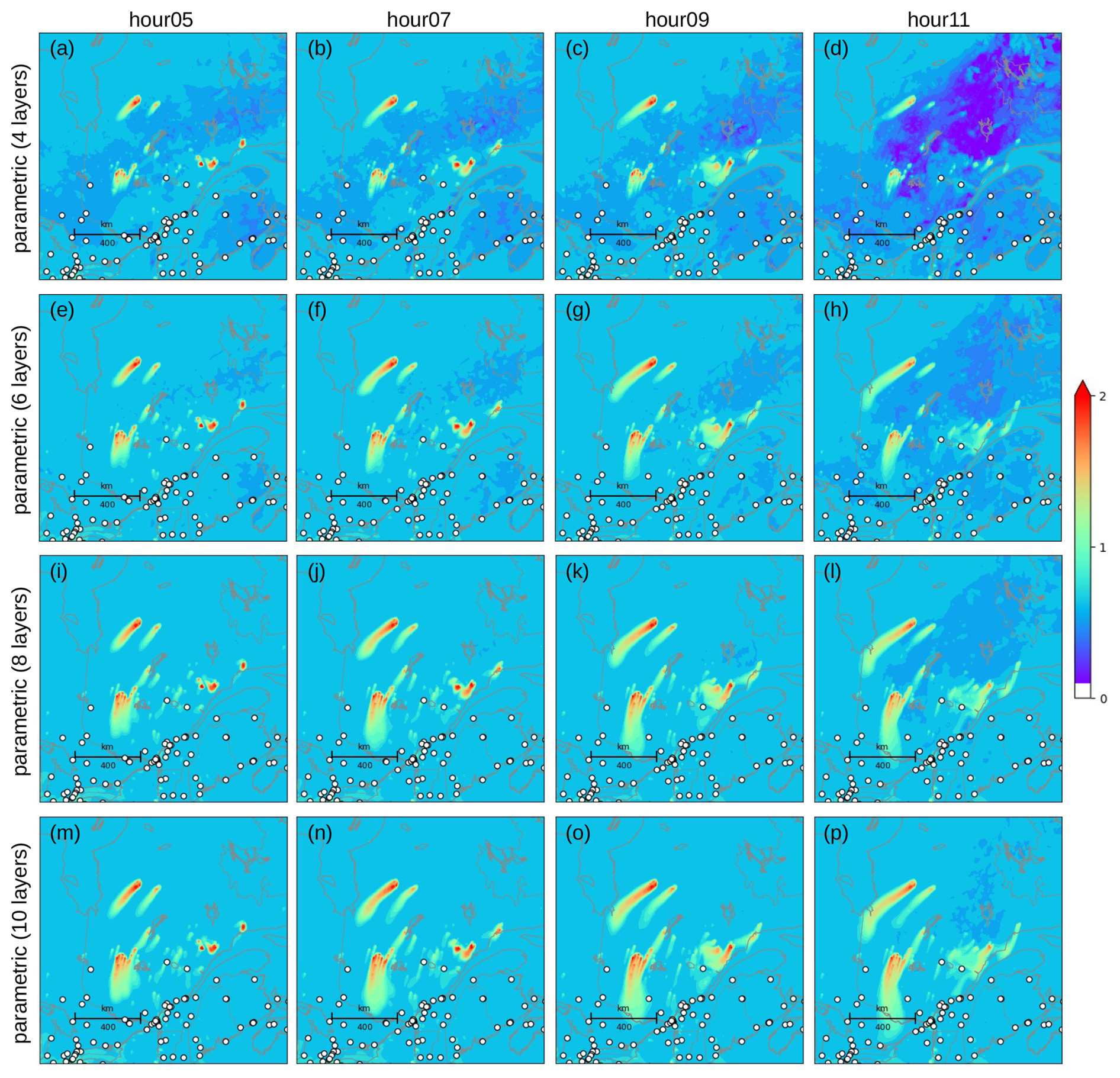
Figure D1 Background error standard deviations fields on 6 June 2023 (logarithmic color code, colorbar labels represent exponent in log ₁₀ (µg m⁻³), hours in UTC) from parametric forecast with different vertical error correlation lengths $L_{\mathit{\xi }}^z(\mathit{x},t)=\mathrm{4};\mathrm{6};\mathrm{8};\mathrm{10}$ model layers. Assimilated surface observations are overplotted as white dots.

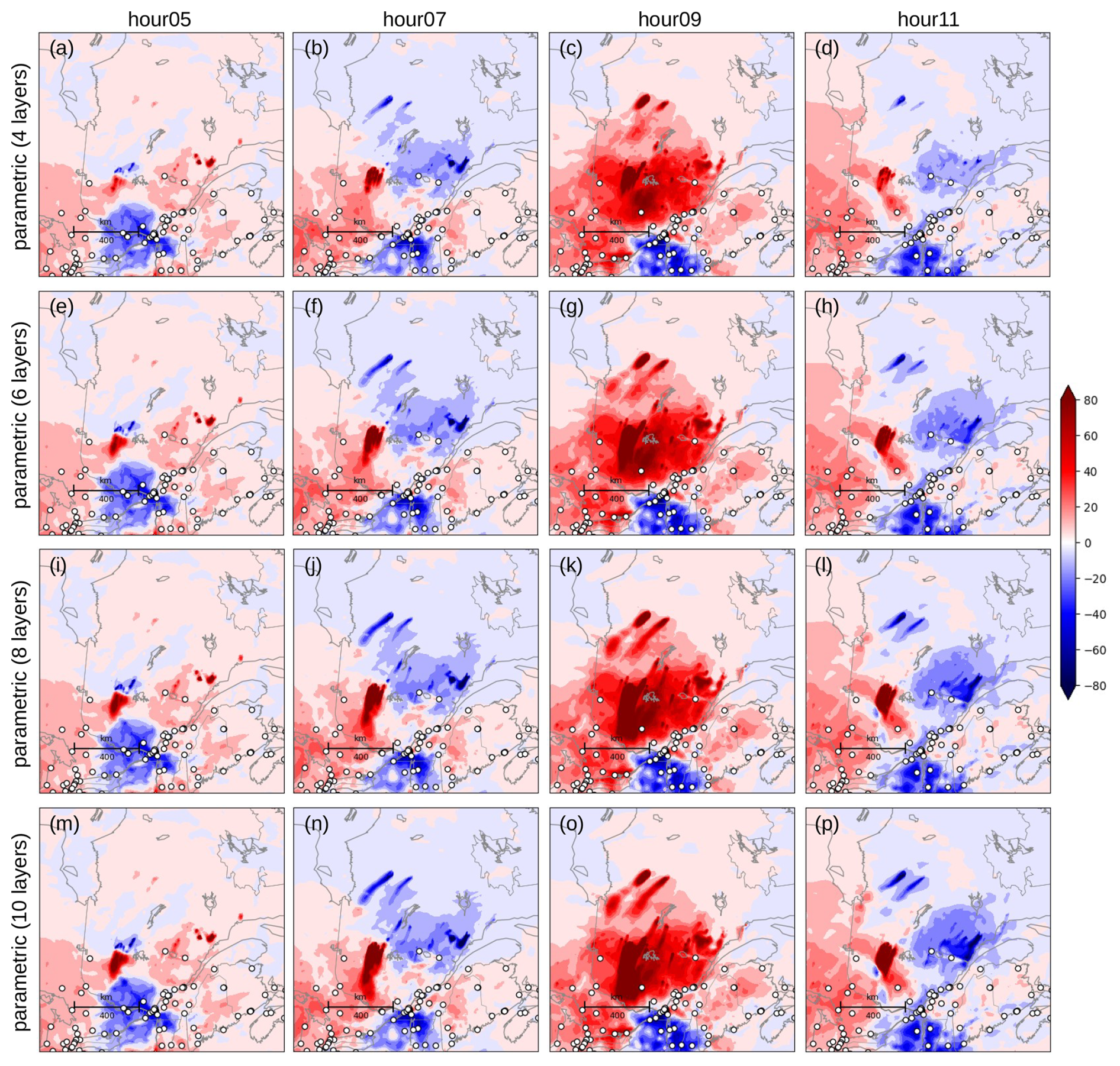
Figure D2 Analysis increments on 6 June 2023 (linear color code, colorbar labels give analysis-background increments in µg m⁻³, hours in UTC) from parametric forecast with different vertical error correlation lengths $L_{\mathit{\xi }}^z(\mathit{x},t)=\mathrm{4};\mathrm{6};\mathrm{8};\mathrm{10}$ model layers. Assimilated surface observations are overplotted as white dots.