Bayesian inference based on algorithms: MH, HMC, MALA and Lip-MALA for prestack seismic inversion

Seismic inversion for estimating elastic properties is a key technique for reservoir characterization after drilling. The choice of inversion method strongly influences the accuracy, efficiency, and reliability of results. Bayesian inference based on Markov Chain Monte Carlo (MCMC) algorithms provides a robust framework for incorporating data uncertainty and prior geological knowledge. In this study, we compare the performance of four inversion methods – Metropolis-Hastings (MH), Hamiltonian Monte Carlo (HMC), the Metropolis-Adjusted Langevin Algorithm (MALA), and its variant Lip-MALA – in prestack seismic inversion using both synthetic models and real data from an eastern Venezuelan hydrocarbon reservoir. Results indicate that gradient-based methods (HMC, MALA, Lip-MALA) outperform MH in velocity estimation, while density inversion remains more challenging. MH and MALA achieve shorter execution times, whereas HMC and Lip-MALA improve accuracy at higher computational cost. This analysis evaluates mean values and standard deviation (SD) estimates for P-wave velocity, S-wave velocity, and density, with quality assessed through correlation metrics, objective function behavior, seismic traces, and Root Mean Square Error (RMSE). A two-dimensional inversion with real data further demonstrates algorithms performance under complex geological conditions. The findings highlight trade-offs between accuracy and efficiency, providing practical guidelines for selecting inversion method in seismic reservoir characterization.

1 Introduction

The accurate characterization of hydrocarbon reservoirs is fundamental for effective exploration and production decisions. This requires integrating complementary sources of information: general geological knowledge from analogous reservoirs and rock physics principles, and reservoir-specific observations from well logs, seismic surveys, and production history.

Seismic data play a central role due to their extensive spatial coverage, providing a continuous description of the subsurface beyond individual well locations. To translate seismic amplitudes into meaningful elastic and petrophysical properties, such as P-wave velocity (V_p), S-wave velocity (V_s), and density (ρ), seismic inversion is employed. This geophysical inverse problem aims to infer subsurface properties from observed seismic data, typically expressed as (Tarantola, 2005):

$$\begin{array}{}\text{(1)}& {\mathit{d}}_{\mathrm{obs}}=g\left(\mathit{m}\right)+\mathit{\xi }\end{array}$$

where d_obs are the observed data, g is the forward operator linking the model parameters m to the data, and ξ represents measurement and modeling errors.

Traditional seismic inversion methods can be broadly categorized into deterministic and stochastic approaches. Deterministic methods, such as least-squares inversion (Tarantola, 2005) and gradient-based optimization (Buland and Omre, 2003), provide single best-fit models but often lack robust uncertainty quantification. Stochastic methods, including simulated annealing (Ma, 2002) and genetic algorithms, explore the model space more broadly but can be computationally intensive and may not guarantee convergence to the posterior distribution.

In prestack amplitude versus offset (AVO) inversion (Helland-Hansen et al., 1997; Ma, 2002; Buland and Omre, 2003), the problem is ill-posed: solutions are non-unique and highly sensitive to data noise and modeling errors (Landa and Treitel, 2016). The elastic parameters $\left(V_{\mathrm{p}},V_{\mathrm{s}},\mathit{\rho }\right)$, from which Lamé parameters can be derived. These are sensitive to rock fluid content and saturation (Clochard et al., 2009) and can be further related to petrophysical parameters such as porosity, sand $/$ shale ratio, and gas saturation (Goodway, 2001). Accurately estimating these parameters is therefore crucial for identifying hydrocarbon accumulations.

To address these challenges, Bayesian inference has emerged as a powerful framework, as it explicitly incorporates prior geological knowledge and quantifies uncertainty through the posterior distribution. Markov Chain Monte Carlo (MCMC) methods are particularly well-suited for sampling complex, high-dimensional posterior distributions in nonlinear inverse problems (Bosch et al., 2007).

Several MCMC algorithms have been applied in geophysical inversion. The Metropolis–Hastings (MH) algorithm (Metropolis et al., 1953; Hastings, 1970) is a foundational method but can suffer from slow convergence in high-dimensional spaces. Hamiltonian Monte Carlo (HMC) (Duane et al., 1987; Neal, 2012) leverages gradient information to propose more efficient moves, making it suitable for high-dimensional problems, as demonstrated in full-waveform inversion (Gebraad et al., 2020) and acoustic inversion (de Lima et al., 2023). Langevin dynamics-based methods, such as the Metropolis-Adjusted Langevin Algorithm (MALA) (Roberts and Tweedie, 1996) and its adaptive variant Lip-MALA (Nemeth and Fearnhead, 2021; Izzatullah et al., 2021), use gradient information to guide proposals, improving mixing and convergence in complex posteriors.

Despite these advances, a systematic comparison of these MCMC algorithms in the context of prestack seismic inversion – particularly using both synthetic and real data in 1D and 2D settings – remains limited. Most studies focus on a single algorithm or synthetic cases, leaving a gap in understanding their practical performance under realistic geological complexity and computational constraints.

This study aims to fill this gap by conducting a comprehensive evaluation of four MCMC algorithms – MH, HMC, MALA, and Lip-MALA – for Bayesian prestack seismic inversion. We assess their performance in estimating elastic parameters (V_p, V_s, ρ) using both noise-free synthetic data and real data from an eastern Venezuelan reservoir. Our analysis includes:

• Quantitative metrics: mean, standard deviation, correlation, and RMSE.

• Computational efficiency: acceptance rates and execution times.

• Convergence diagnostics: multivariate effective sample size (mESS).

• Practical applicability: extension to 2D inversion with real data.

Our contributions are threefold:

1. We provide a benchmark comparison of MCMC algorithms in seismic inversion, highlighting trade-offs between accuracy, uncertainty quantification, and computational cost.

2. We demonstrate the scalability of these methods from 1D to 2D real-data scenarios, validating their robustness in geologically complex settings.

3. We offer practical guidelines for algorithm selection based on project requirements, data characteristics, and available computational resources.

In Prestack AVO, Bayesian approaches with MCMC have been previously applied to estimate impedance or elastic parameters (e.g., Bosch et al., 2007; Wu et al., 2019), but these studies focus on a single algorithm or mainly on synthetic cases, but we go further and test it on real data.

The remainder of this paper is organized as follows: Sect. 2 formulates the seismic inversion problem within a Bayesian framework and describes the forward modeling approach based on AVO theory. Section 3 details the theoretical background of the MCMC algorithms. Section 4 presents result from synthetic and real data experiments. Section 5 discusses the implications and practical recommendations. Section 6 concludes the study.

2 The Seismic Inversion Problem

Having established the importance of Bayesian MCMC methods for prestack seismic inversion in Sect. 1, this section provides a comprehensive formulation of the inverse problem within a rigorous statistical framework. We detail the mathematical foundations, model parameterization, forward modeling approach, and inference workflow that form the basis of our comparative study. The complete Bayesian inference flow implemented in this study is visually summarized in Fig. 1, which illustrates the steps from input data to subsequent uncertainty quantification.

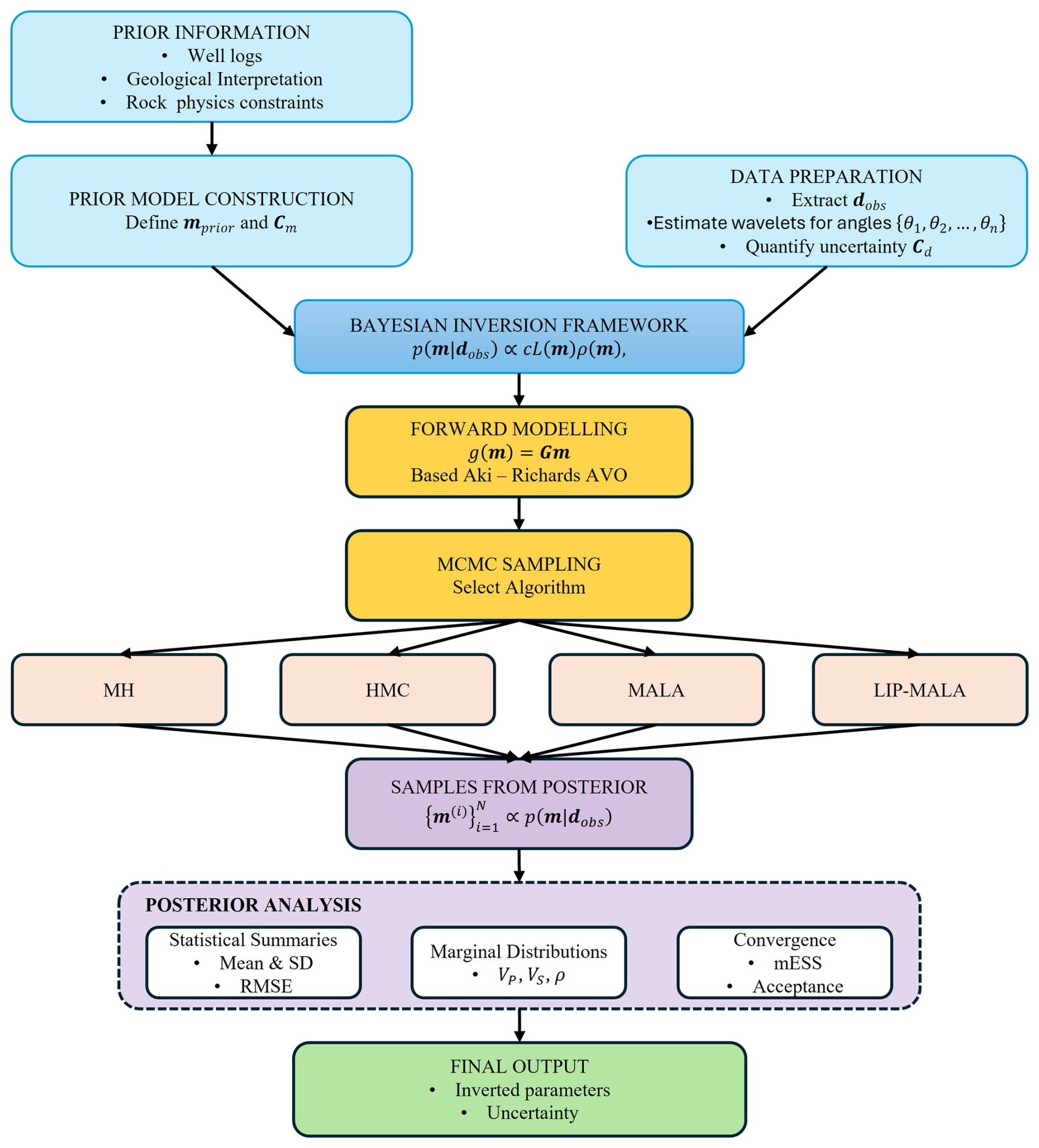
Figure 1 Bayesian seismic inversion workflow implemented in this study, integrating prior information, seismic data, forward modelling, MCMC sampling, and posterior analysis to produce probabilistic estimates of elastic parameters with quantified uncertainties.

2.1 Bayesian Formulation of the Inverse Problem

Within the Bayesian paradigm, the solution to the inverse problem is expressed probabilistically through the posterior distribution (Tarantola, 2005; Bosch et al., 2007) p(m|d_obs), which combines prior knowledge with information from the observed data. Applying Bayes' theorem, we have:

$$\begin{array}{}\text{(2)}& p\left(\mathit{m}\mathrm{|}{\mathit{d}}_{\mathrm{obs}}\right)={\displaystyle \frac{p\left({\mathit{d}}_{\mathrm{obs}}\mathrm{|}\mathit{m}\right)p\left(\mathit{m}\right)}{p\left({\mathit{d}}_{\mathrm{obs}}\right)}}\propto cL\left(\mathit{m}\right)\mathit{\rho }\left(\mathit{m}\right),\end{array}$$

where:

• ρ(m) is the prior distribution, representing geological knowledge independent of the seismic data.

• L(m) is the likelihood function, quantifying the probability of observing the data given a specific model.

• c is a normalization constant.

• And $p\left({\mathit{d}}_{\mathrm{obs}}\right)=\int p\left({\mathit{d}}_{\mathrm{obs}}\mathrm{|}\mathit{m}\right)p\left(\mathit{m}\right)d\mathit{m}$

2.1.1 Prior Distribution Specification

The prior distribution encodes constraints on the model parameters based on independent information such as well logs, regional geology, and rock physics relationships. We employ a Gaussian prior distribution $\mathit{\rho }\left(\mathit{m}\right)\sim N\left({\mathit{m}}_{\mathrm{prior}},{\mathbf{C}}_{\mathrm{m}}\right)$ (Bosch, 2004; Buland and Omre, 2003):

$$\begin{array}{}\text{(3)}& \mathit{\rho }\left(\mathit{m}\right)=c_{\mathrm{1}}\exp \left[-{\displaystyle \frac{\mathrm{1}}{\mathrm{2}}}{\left(\mathit{m}-{\mathit{m}}_{\mathrm{prior}}\right)}^T{\mathbf{C}}_{\mathrm{m}}^{-\mathrm{1}}\left(\mathit{m}-{\mathit{m}}_{\mathrm{prior}}\right)\right],\end{array}$$

where N denotes a Gaussian probability distribution, with mean ${\mathit{m}}_{\mathrm{prior}}\in R^{N_{\mathrm{m}}}$, typically derived from low-frequency interpolation of well data or seismic velocities, covariance matrix given by ${\mathbf{C}}_{\mathrm{m}}\in R^{N_{\mathrm{m}}\times N_{\mathrm{m}}}$, which imposes spatial correlation and smoothness constraints, effectively regularizing the ill-posed inverse problem and c₁ an appropriate normalization constant.

2.1.2 Likelihood Function and Data Errors

Assuming Gaussian-distributed errors in Eq. (1) with zero mean and covariance matrix C_d, the likelihood function takes the form:

$$\begin{array}{}\text{(4)}& L\left(\mathit{m}\right)=\exp \left[-{\displaystyle \frac{\mathrm{1}}{\mathrm{2}}}{\left({\mathit{d}}_{\mathrm{obs}}-g\left(\mathit{m}\right)\right)}^T{\mathbf{C}}_{\mathrm{d}}^{-\mathrm{1}}\left({\mathit{d}}_{\mathrm{obs}}-g\left(\mathit{m}\right)\right)\right],\end{array}$$

The likelihood function assumes Gaussian-distributed errors, consistent with standard formulations in Bayesian seismic inversion (Tarantola, 2005; Izzatullah et al., 2021), $g:\mathit{m}\to {\mathit{d}}_{\mathrm{obs}}$, being the function solving the seismic forward problem and the data covariance matrix C_d accounts for measurement noise and uncertainties in the forward model. While often assumed diagonal (uncorrelated errors), it can incorporate more complex error structures when available.

2.1.3 Posterior Distribution and MCMC Sampling

Combining Eqs. (3) and (4), the posterior distribution can be expressed through the negative log-posterior (misfit function) S(m):

$$\begin{array}{}\text{(5)}& \begin{array}{rl}S\left(\mathit{m}\right)& =-\log p\left(\mathit{m}\mathrm{|}{\mathit{d}}_{\mathrm{obs}}\right)\\ & ={\displaystyle \frac{\mathrm{1}}{\mathrm{2}}}{\left({\mathit{d}}_{\mathrm{obs}}-g\left(\mathit{m}\right)\right)}^T{\mathbf{C}}_{\mathrm{d}}^{-\mathrm{1}}\left({\mathit{d}}_{\mathrm{obs}}-g\left(\mathit{m}\right)\right)\\ & +{\displaystyle \frac{\mathrm{1}}{\mathrm{2}}}{\left(\mathit{m}-{\mathit{m}}_{\mathrm{prior}}\right)}^T{\mathbf{C}}_{\mathrm{m}}^{-\mathrm{1}}\left(\mathit{m}-{\mathit{m}}_{\mathrm{prior}}\right),\end{array}\end{array}$$

Thus,

$$\begin{array}{}\text{(6)}& p\left(\mathit{m}\mathrm{|}{\mathit{d}}_{\mathrm{obs}}\right)\propto \exp \left[-S\left(\mathit{m}\right)\right],\end{array}$$

In practice, the posterior distribution defined above is analytically intractable. Markov Chain Monte Carlo (MCMC) methods are therefore employed to generate samples ${\left\{{\mathit{m}}^{\left(i\right)}\right\}}_{i=\mathrm{1}}^N$ from Eq. (6), enabling comprehensive uncertainty quantification through estimation of posterior means, variances, and marginal distributions (Robert and Casella, 2004; Neal, 2012; Gebraad et al., 2020).

2.2 Model Parameterization and Forward Modelling

2.2.1 Logarithmic Parameterization

To ensure positivity of physical parameters (V_p>0, V_s>0, ρ>0) and improve numerical stability, we adopt a logarithmic parameterization. For a 1D model with N layers, the parameter vector is (Buland and Omre, 2003):

$$\begin{array}{}\text{(7)}& \begin{array}{rl}\mathit{m}& =[\ln \left(V_{\mathrm{p},\mathrm{1}}\right),\mathrm{\dots },\ln \left(V_{\mathrm{p},\mathrm{N}}\right),\ln \left(V_{\mathrm{s},\mathrm{1}}\right),\mathrm{\dots },\\ & \ln \left(V_{\mathrm{s},\mathrm{N}}\right),\ln \left({\mathit{\rho }}_{\mathrm{1}}\right),\mathrm{\dots },\ln \left({\mathit{\rho }}_{\mathrm{N}}\right){]}^T,\end{array}\end{array}$$

This transformation also aligns naturally with the logarithmic form of the Aki-Richards reflectivity approximation used in our forward model.

2.2.2 AVO Forward Modeling Formulation

The forward operator g(m) implements the Aki-Richards linearized approximation for PP reflectivity. The AVO method was created in the early 1980s to analyze the amplitudes of seismic CMP gathers as a function of angle to find hydrocarbons. The Aki-Richards equation (Aki and Richards, 2002) is the foundation of AVO analysis. The original form of the equation can be rewritten for a weak-contrast interface to give (Buland and Omre, 2003; Niu et al., 2020):

$$\begin{array}{}\text{(8)}& R_{\mathrm{pp}}\left(\mathit{\theta }\right)=c_{\mathrm{1}}\left(\mathit{\theta }\right){\displaystyle \frac{\mathrm{\Delta }{V}_{\mathrm{p}}}{{\stackrel{\mathrm{‾}}{V}}_{\mathrm{p}}}}+c_{\mathrm{2}}\left(\mathit{\theta }\right){\displaystyle \frac{\mathrm{\Delta }{V}_{\mathrm{s}}}{{\stackrel{\mathrm{‾}}{V}}_{\mathrm{s}}}}+c_{\mathrm{3}}\left(\mathit{\theta }\right){\displaystyle \frac{\mathrm{\Delta }\mathit{\rho }}{\stackrel{\mathrm{‾}}{\mathit{\rho }}}},\end{array}$$

where

$$\begin{array}{}\text{(9)}& {\displaystyle }{c}_{\mathrm{1}}\left(\mathit{\theta }\right)={\displaystyle \frac{\mathrm{1}}{\mathrm{2}}}\left(\mathrm{1}+{\tan }^{\mathrm{2}}\mathit{\theta }\right),\text{(10)}& {\displaystyle }{c}_{\mathrm{2}}\left(\mathit{\theta }\right)=-\mathrm{4}{\displaystyle \frac{{\stackrel{\mathrm{‾}}{V}}_{\mathrm{s}}}{{\stackrel{\mathrm{‾}}{V}}_{\mathrm{p}}}}{\sin }^{\mathrm{2}}\mathit{\theta },\text{(11)}& {\displaystyle }{c}_{\mathrm{3}}\left(\mathit{\theta }\right)={\displaystyle \frac{\mathrm{1}}{\mathrm{2}}}\left(\mathrm{1}-\mathrm{4}{\displaystyle \frac{{\stackrel{\mathrm{‾}}{V}}_{\mathrm{s}}}{{\stackrel{\mathrm{‾}}{V}}_{\mathrm{p}}}}{\sin }^{\mathrm{2}}\mathit{\theta }\right),\end{array}$$

In Eqs. (8)–(11), the incident angle θ is the angle at which a wave reflected off a surface. V_p, V_s and ρ represent the velocities of P-waves, S-waves, and the density of a material, respectively. ΔV_p, ΔV_s and Δρ are the changes in V_p, V_s and ρ across a reflective interface. $\stackrel{\mathrm{‾}}{V_{\mathrm{p}}}$, $\stackrel{\mathrm{‾}}{V_{\mathrm{s}}}$ and $\stackrel{\mathrm{‾}}{\mathit{\rho }}$ are the average values of V_p, V_s and ρ, respectively.

To obtain the seismic trace for a certain theta angle we can use the approximation for small reflectivity (Russell et al., 2006),

$$\begin{array}{}\text{(12)}& \begin{array}{rl}T\left(\mathit{\theta }\right)& ={\displaystyle \frac{\mathrm{1}}{\mathrm{2}}}{c}_{\mathrm{1}}\mathbf{W}\left(\mathit{\theta }\right)\mathbf{D}{L}_{V_{\mathrm{p}}}+{\displaystyle \frac{\mathrm{1}}{\mathrm{2}}}{c}_{\mathrm{2}}\mathbf{W}\left(\mathit{\theta }\right)\mathbf{D}{L}_{V_{\mathrm{s}}}\\ & +{\displaystyle \frac{\mathrm{1}}{\mathrm{2}}}{c}_{\mathrm{3}}\mathbf{W}\left(\mathit{\theta }\right)\mathbf{D}{L}_{\mathit{\rho }},\end{array}\end{array}$$

where $L_{V_{\mathrm{p}}}=\ln \left(V_{\mathrm{p}}\right)$, $L_{V_{\mathrm{s}}}=\ln \left(V_{\mathrm{s}}\right)$, L_ρ=ln (ρ), W is the wavelet matrix and D is the derivative matrix. Equation (12) can be implemented in matrix form as

$$\begin{array}{}\text{(13)}& \begin{array}{rl}& \left[\begin{array}{c}T\left({\mathit{\theta }}_{\mathrm{1}}\right)\\ T\left({\mathit{\theta }}_{\mathrm{2}}\right)\\ \mathrm{⋮}\\ T\left({\mathit{\theta }}_n\right)\end{array}\right]=\\ & {\displaystyle \frac{\mathrm{1}}{\mathrm{2}}}\left[\begin{array}{ccc}{c}_{\mathrm{1}}\mathbf{W}\left({\mathit{\theta }}_{\mathrm{1}}\right)\mathbf{D}& c_{\mathrm{2}}\mathbf{W}\left({\mathit{\theta }}_{\mathrm{1}}\right)\mathbf{D}& c_{\mathrm{3}}\mathbf{W}\left({\mathit{\theta }}_{\mathrm{1}}\right)\mathbf{D}\\ c_{\mathrm{1}}\mathbf{W}\left({\mathit{\theta }}_{\mathrm{2}}\right)\mathbf{D}& c_{\mathrm{2}}\mathbf{W}\left({\mathit{\theta }}_{\mathrm{2}}\right)\mathbf{D}& c_{\mathrm{3}}\mathbf{W}\left({\mathit{\theta }}_{\mathrm{2}}\right)\mathbf{D}\\ \mathrm{⋮}& \mathrm{⋮}& \mathrm{⋮}\\ c_{\mathrm{1}}\mathbf{W}\left({\mathit{\theta }}_n\right)\mathbf{D}& c_{\mathrm{2}}\mathbf{W}\left({\mathit{\theta }}_n\right)\mathbf{D}& c_{\mathrm{3}}\mathbf{W}\left({\mathit{\theta }}_n\right)\mathbf{D}\end{array}\right]\left[\begin{array}{c}{L}_{V_{\mathrm{p}}}\\ L_{V_{\mathrm{s}}}\\ L_{\mathit{\rho }}\end{array}\right]\end{array}\end{array}$$

In discrete matrix form, for multiple angles $\left\{{\mathit{\theta }}_{\mathrm{1}},{\mathit{\theta }}_{\mathrm{2}},\mathrm{\dots },{\mathit{\theta }}_n\right\}$, the complete forward modeling operation can be expressed compactly as:

$$\begin{array}{}\text{(14)}& {\mathit{d}}_{\mathrm{syn}}=g\left(\mathit{m}\right)=\mathbf{G}\mathit{m},\end{array}$$

where:

$$\begin{array}{}\text{(15)}& \begin{array}{rl}& {\mathit{d}}_{\mathrm{syn}}=\left[\begin{array}{c}T\left({\mathit{\theta }}_{\mathrm{1}}\right)\\ T\left({\mathit{\theta }}_{\mathrm{2}}\right)\\ \mathrm{⋮}\\ T\left({\mathit{\theta }}_n\right)\end{array}\right];\\ & \mathbf{G}={\displaystyle \frac{\mathrm{1}}{\mathrm{2}}}\left[\begin{array}{ccc}{c}_{\mathrm{1}}\mathbf{W}\left({\mathit{\theta }}_{\mathrm{1}}\right)\mathbf{D}& c_{\mathrm{2}}\mathbf{W}\left({\mathit{\theta }}_{\mathrm{1}}\right)\mathbf{D}& c_{\mathrm{3}}\mathbf{W}\left({\mathit{\theta }}_{\mathrm{1}}\right)\mathbf{D}\\ c_{\mathrm{1}}\mathbf{W}\left({\mathit{\theta }}_{\mathrm{2}}\right)\mathbf{D}& c_{\mathrm{2}}\mathbf{W}\left({\mathit{\theta }}_{\mathrm{2}}\right)\mathbf{D}& c_{\mathrm{3}}\mathbf{W}\left({\mathit{\theta }}_{\mathrm{2}}\right)\mathbf{D}\\ \mathrm{⋮}& \mathrm{⋮}& \mathrm{⋮}\\ c_{\mathrm{1}}\mathbf{W}\left({\mathit{\theta }}_n\right)D& c_{\mathrm{2}}\mathbf{W}\left({\mathit{\theta }}_n\right)\mathbf{D}& c_{\mathrm{3}}\mathbf{W}\left({\mathit{\theta }}_n\right)\mathbf{D}\end{array}\right]\end{array}\end{array}$$

and m was defined in Eq. (7). For how to construct W and D, known as the wavelet matrix and the derivative matrix respectively, the reader is advised to review Hampson et al. (2005).

2.3 Inference Workflow and Uncertainty Quantification

The complete Bayesian inversion workflow implemented in this study is visually summarized in Fig. 1. The process integrates prior geological knowledge, seismic data, physical modelling, and statistical sampling to produce probabilistic estimates of subsurface elastic properties.

Bayesian inversion process implemented in this study follows a systematic workflow:

1. Prior Model Construction: Define m_prior and C_m using available well-log data, geological interpretation, and spatial correlation models.

2. Data Preparation and Uncertainty Quantification: Extract angle-stacked seismic traces d_obs, estimate corresponding wavelets for multiple angles $\left\{{\mathit{\theta }}_{\mathrm{1}},{\mathit{\theta }}_{\mathrm{2}},\mathrm{\dots },{\mathit{\theta }}_n\right\}$, and characterize data uncertainties through the covariance matrix C_d

3. Forward Operator Assembly: Construct the matrix G according to Eqs. (8)–(15) to implement the forward modelling operator g(m).

4. MCMC Sampling: Apply one of the four sampling algorithms (MH, HMC, MALA, or Lip-MALA) to generate a Markov chain of model samples from the posterior distribution p(m|d_obs)

5. Posterior Analysis: Compute statistical summaries (posterior means, standard deviations, correlation coefficients, RMSE) and marginal probability distributions from the sampled models to assess the inverted elastic parameters and their associated uncertainties.

This comprehensive framework provides a rigorous approach to seismic inversion where solutions are characterized not as single models but as probability distributions that fully quantify uncertainty, directly addressing the ill-posed nature of the inverse problem.

3 Theoretical Background for Metropolis-Hastings, Hamiltonian Monte Carlo and Langevin Diffusion

This section presents the theoretical foundations of the four MCMC algorithms compared in this study. A visual summary of their computational workflows and key characteristics is provided in Fig. 2, followed by detailed mathematical descriptions and implementation considerations.

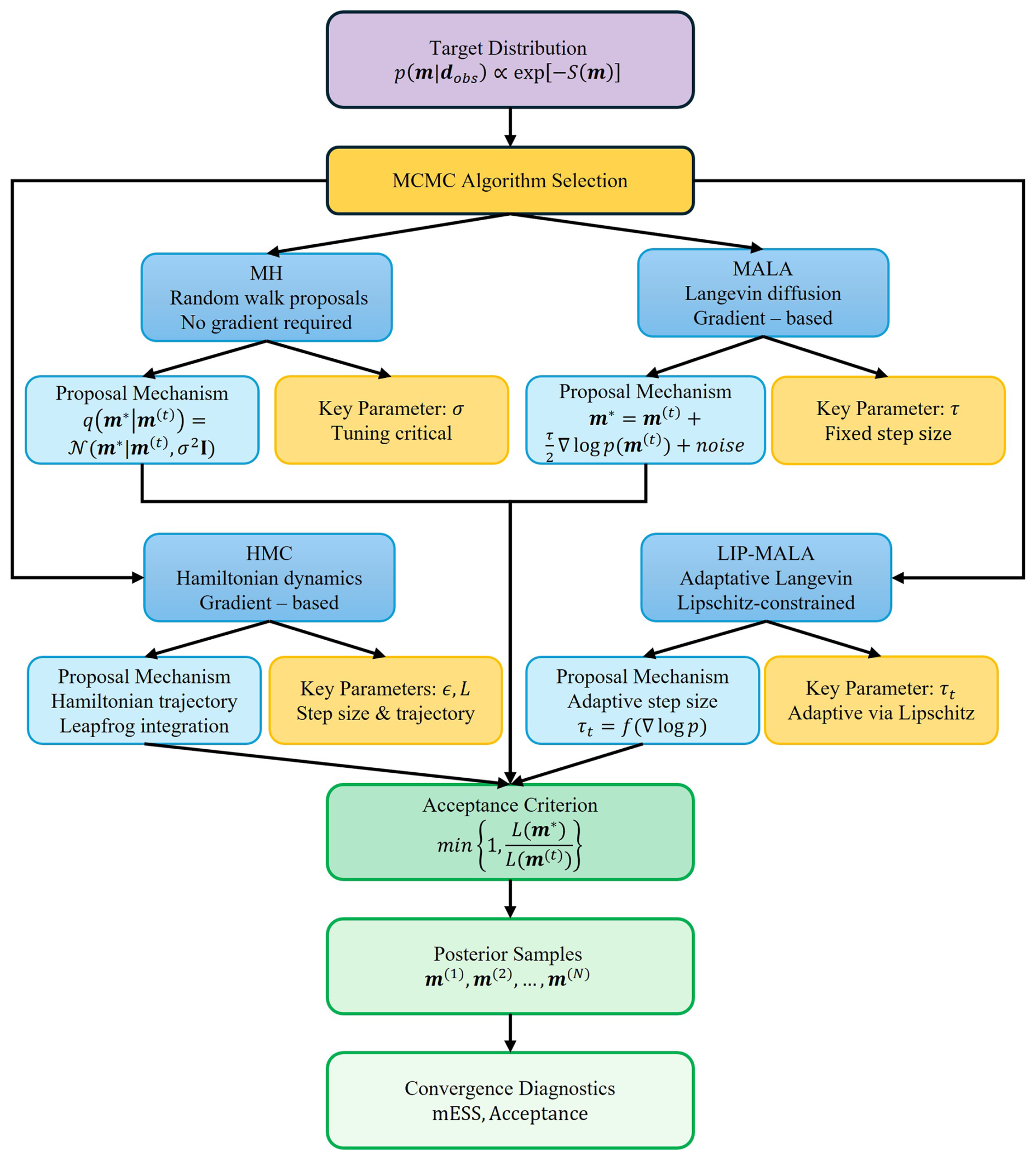
Figure 2 Comparative schematic of MCMC algorithms evaluated in this study. All methods generate samples from the posterior distribution but differ in proposal mechanisms, gradient requirements, and parameter tuning strategies.

3.1 Algorithm Overview and Comparative Framework

Figure 2 provides a schematic comparative view of the four MCMC algorithms, highlighting their proposal mechanisms, gradient requirements, and tuning strategies. All methods share the common goal of generating samples from the posterior distribution p(m|d_obs) but employ different strategies for proposing and accepting new states.

3.2 Metropolis–Hastings Algorithm

MH algorithm is one of the most widely used MCMC methods for sampling from complex probability distributions. Originally proposed by Metropolis et al. (1953) and generalized by Hastings (1970), MH defines a transition probability that ensures ergodicity, detailed balance, and reversibility of the chain (Chib and Greenberg, 1995).

3.2.1 Mathematical Formulation

Given the current state m^(t) at iteration t, MH proposes a new candidate m^∗ from a proposal distribution q(m^∗|m^(t)). The candidate is accepted with probability:

$$\begin{array}{}\text{(16)}& {\mathit{\alpha }}_{\mathrm{MH}}=min\left\{\mathrm{1},{\displaystyle \frac{L\left({\mathit{m}}^{\ast }\right)}{L\left({\mathit{m}}^{\left(t\right)}\right)}}\cdot {\displaystyle \frac{q\left({\mathit{m}}^{\left(t\right)}\mathrm{|}{\mathit{m}}^{\ast }\right)}{q\left({\mathit{m}}^{\ast }\mathrm{|}{\mathit{m}}^{\left(t\right)}\right)}}\right\},\end{array}$$

where L(⋅) represents the likelihood function (Eq. 4). For symmetric proposal distributions where $q\left({\mathit{m}}^{\ast }\mathrm{|}{\mathit{m}}^{\left(t\right)}\right)=q\left({\mathit{m}}^{\left(t\right)}\mathrm{|}{\mathit{m}}^{\ast }\right)$, this simplifies to the Metropolis acceptance ratio.

Implementation Details

In our seismic inversion context, we employ a Gaussian random walk proposal:

$$\begin{array}{}\text{(17)}& q\left({\mathit{m}}^{\ast }\mathrm{|}{\mathit{m}}^{\left(t\right)}\right)=N\left({\mathit{m}}^{\ast }\mathrm{|}{\mathit{m}}^{\left(t\right)},{\mathit{\sigma }}^{\mathrm{2}}\mathbf{I}\right),\end{array}$$

Where σ is a tuning parameter controlling the proposal step size. The algorithm proceeds as follows:

•  

  Step 1. Initialization: Start with an initial model m⁽⁰⁾=m_prior and set t=0.

•  

  Step 2. Propose a new state: Generate ${\mathit{m}}^{\ast }\sim N\left({\mathit{m}}^{\left(t\right)},{\mathit{\sigma }}^{\mathrm{2}}\mathbf{I}\right)$.

•  

  Step 3. Compute Acceptance: Calculate α_MH using Eq. (16).

•  

  Step 4. Accept/Reject: Draw $u\sim \mathrm{Uniform}\left(\mathrm{0},\mathrm{1}\right)$. If u≤α_MH, set ${\mathit{m}}^{\left(t+\mathrm{1}\right)}={\mathit{m}}^{\ast }$; otherwise ${\mathit{m}}^{\left(t+\mathrm{1}\right)}={\mathit{m}}^{\left(t\right)}$

•  

  Step 5. Iterate: Increment t and repeat from step 2 until convergence.

3.2.2 Tuning Considerations and Limitations

The performance of MH critically depends on the choice of σ. Optimal scaling theory suggests aiming for acceptance rates of approximately 23.4 % for random walk proposals in high dimensions (Roberts et al., 1997). In our implementation, σ was tuned during a 1000-iteration burn-in period to achieve this target.

While MH is conceptually simple and requires no gradient computations, its random walk behavior leads to slow exploration of high-dimensional parameter spaces. The autocorrelation between samples remains high, requiring longer chains to achieve effective sample sizes comparable to gradient-based methods.

3.3 Hamiltonian Monte Carlo (HMC)

HMC is a sampling algorithm that was first introduced in molecular dynamics (Duane et al., 1987) and later adapted to Bayesian inference problems (Neal, 2012; Fichtner and Zunino, 2019). It is particularly effective for high-dimensional posteriors when gradient information of the σ is available and it is more efficient than standard MH. It introduces an auxiliary momentum variable to simulate Hamiltonian dynamics in an augmented parameter space.

3.3.1 Hamiltonian Dynamics Formulation

HMC is an MCMC algorithm that uses classical Hamiltonian mechanics (Landau and Lifshitz, 1976) to sample from an arbitrary n-dimensional probability density function (PDF). HMC introduces momentum variables $\mathit{p}\mathit{ϵ}{R}^{N_{\mathrm{m}}}$ and samples from the joint distribution:

$$\begin{array}{}\text{(18)}& p\left(\mathit{m}\mathbf{,}\mathit{p}\right)=p\left(\mathit{m}\right)p\left(\mathit{p}\right)\propto \exp \left(-U\left(\mathit{m}\right)-K\left(\mathit{p}\right)\right)\end{array}$$

where $U\left(\mathit{m}\right)=-\log \left(p\left(\mathit{m}\right)\right)$ , which is defined as the negative logarithm of the PDF (Gebraad et al., 2020), and $K\left(\mathit{p}\right)=\frac{\mathrm{1}}{\mathrm{2}}{\mathit{p}}^T{\mathbf{M}}^{-\mathrm{1}}\mathit{p}$ is the kinetic energy with mass matrix M.

The Hamiltonian equations of motion are:

$$\begin{array}{}\text{(19)}& {\displaystyle \frac{\mathrm{d}\mathit{m}}{\mathrm{d}\mathit{\tau }}}={\displaystyle \frac{\partial H}{\partial \mathit{p}}}={\mathbf{M}}^{-\mathrm{1}}\mathit{p},{\displaystyle \frac{\mathrm{d}\mathit{p}}{\mathrm{d}\mathit{\tau }}}=-{\displaystyle \frac{\partial H}{\partial \mathit{m}}}=-\mathrm{\nabla }U\left(\mathit{m}\right)\end{array}$$

where $H\left(\mathit{m},\mathit{p}\right)=U\left(\mathit{m}\right)+K\left(\mathit{p}\right)$ is the Hamiltonian and τ is fictitious time.

3.3.2 Leapfrog Integration and Algorithm

Since analytical solutions to Eq. (19) are unavailable for nonlinear problems, HMC employs the symplectic leapfrog integrator with step size ϵ and L steps. For our seismic inversion, the algorithm proceeds as (Gebraad et al., 2020):

•  

  Step 1. Start with an initial model m⁽⁰⁾=m_prior, random momenta p⁽⁰⁾∼N(M). and set t=0.

•  

  Step 2. Evaluate the Hamiltonian H(m^(t)p^(t)) starting with t=0.

•  

  Step 3. Leapfrog integration (repeated L times): Calculate:

  $$\begin{array}{}\text{(20)}& {\displaystyle }{\mathit{p}}^{\ast }={\mathit{p}}^{\left(t\right)}-{\displaystyle \frac{\mathit{ϵ}}{\mathrm{2}}}\mathrm{\nabla }U\left({\mathit{m}}^{\left(t\right)}\right)\text{(21)}& {\displaystyle }{\mathit{m}}^{\ast }={\mathit{m}}^{\left(t\right)}+\mathit{ϵ}{\mathit{p}}^{\ast }\text{(22)}& {\displaystyle }{\mathit{p}}^{\ast }={\mathit{p}}^{\ast }-{\displaystyle \frac{\mathit{ϵ}}{\mathrm{2}}}\mathrm{\nabla }U\left({\mathit{m}}^{\ast }\right)\end{array}$$
•  

  Step 4. Calculate the Hamiltonian $H\left({\mathit{m}}^{\ast }{\mathit{p}}^{\ast }\right)$.

•  

  Step 5. Compute Acceptance: Calculate α_HMC using:

  $$\begin{array}{}\text{(23)}& {\mathit{\alpha }}_{\mathrm{HMC}}=min\left(\mathrm{1},\exp \left(H({\mathit{m}}^{\left(t\right)},{\mathit{p}}^{\left(t\right)})-H({\mathit{m}}^{\ast },{\mathit{p}}^{\ast })\right)\right),\end{array}$$
•  

  Step 6. Accept/Reject: Draw $u\sim \mathrm{Uniform}\left(\mathrm{0},\mathrm{1}\right)$. If u≤α_HMC, set ${\mathit{m}}^{\left(t+\mathrm{1}\right)}={\mathit{m}}^{\ast }$ and $H\left({\mathit{m}}^{\left(t+\mathrm{1}\right)},{\mathit{p}}^{\left(t+\mathrm{1}\right)}\right)=H\left({\mathit{m}}^{\ast }{\mathit{p}}^{\ast }\right)$; otherwise ${\mathit{m}}^{\left(t+\mathrm{1}\right)}={\mathit{m}}^{\left(t\right)}$and ${\mathit{p}}^{\left(t+\mathrm{1}\right)}\sim N\left(\mathrm{0},\mathbf{M}\right)$

•  

  Step 7. Iterate: Increment t and repeat from step 2 until convergence.

The acceptance rate of the leapfrog integration algorithm commonly used in Step 3 is largely influenced by how well it conserves energy in the trajectory. If the time steps are too large or the gradients of the fitting function are incorrectly calculated, the algorithm will save less energy, and the acceptance rate will decrease. Simply put, the leapfrog integration algorithm works by bouncing model parameters back and forth across the simulated energy landscape. The acceptance rate determines how often the algorithm accepts a new proposed model parameter. If the time steps are too large or the gradients are calculated incorrectly, the algorithm cannot follow the energy landscape accurately and will likely reject the proposed model parameters. This leads to slower convergence and increases computational cost.

3.3.3 Parameter Tuning for Seismic Inversion

HMC requires careful tuning of two parameters: the step size ϵ and trajectory length L. We employed a dual adaptation strategy:

1. Step size (ϵ): Tuned during burn-in to achieve acceptance rates optimal for HMC.

2. Trajectory length (L): Fixed at L=10 based on preliminary experiments showing adequate exploration without excessive computational cost.

3.4 Langevin Diffusion-Based Algorithms

3.4.1 Langevin Dynamics

Langevin dynamics are a mathematical model of Brownian motion, named after the French physicist Paul Langevin (Lemons and Gythiel, 1997) who developed them in 1908. Langevin dynamics is a simplification of Albert Einstein's approach to Brownian motion, which is based on Newton's second law of motion. The Langevin dynamics for target distribution σ(m_t), is a continuous-time stochastic process ${\left({\mathit{m}}_t\right)}_{t\ge \mathrm{0}}$ in $R^{N_{\mathrm{m}}}$ that evolves following the stochastic differential equation (SDE) (Roberts and Stramer, 2002; Nemeth et al., 2016; Izzatullah et al., 2021) and (Sánchez et al., 2016; Infante et al., 2019):

$$\begin{array}{}\text{(24)}& \mathrm{d}\mathit{m}\left(\mathit{\tau }\right)=-\mathbf{\Sigma }\mathrm{\nabla }\log \left[p\left(\mathit{m}\left(\mathit{\tau }\right)\right)\right]\mathrm{d}\mathit{\tau }+\sqrt{\mathrm{2}}{\mathbf{\Sigma }}^{\frac{-\mathrm{1}}{\mathrm{2}}}\mathrm{d}\mathbf{W}\left(\mathit{\tau }\right)\end{array}$$

where W(τ) is a standard n-dimensional Brownian motion, Σ is a symmetric positive definite matrix (in this paper we use Σ=I), ∇log [σ(m_t)] is the drift term of the Brownian particle m_t and σ(m_t) is a stationary posterior distribution.

3.4.2 Metropolis-adjusted Langevin algorithm (MALA)

In the practice, a standard approach is to discretize the Eq. (13) using the Euler-Maruyama discretization (Stuart et al., 2004) and we obtained the Unadjusted Langevin algorithm (ULA) given by

$$\begin{array}{}\text{(25)}& \begin{array}{rl}& {\mathit{m}}^{\ast }={\mathit{m}}^{\left(t\right)}+\mathit{\tau }\mathbf{\Sigma }\mathrm{\nabla }\log \left[p\left({\mathit{m}}^{\left(t\right)}\right)\right]+\sqrt{\mathrm{2}\mathit{\tau }}{\mathrm{\Sigma }}^{\frac{-\mathrm{1}}{\mathrm{2}}}{\mathit{ϵ}}_t,\\ & {\mathit{ϵ}}_t\sim N\left(\mathrm{0},I_{n\times n}\right)\end{array}\end{array}$$

where τ is the step-length for each iteration. ULA is simple in its implementation, yet it introduces a bias, then we need to introduce the acceptance-rejection step through the MH algorithm. By introducing MH algorithm into ULA, we will obtain the Metropolis-Adjusted Langevin algorithm (MALA), (Izzatullah et al., 2020, 2021). The procedure consists of constructing a Markov chain at each step t, given m^(t), a new observation is generated from a proposal density q(m^∗). The candidate is then accepted with probability α_MALA given by,

$$\begin{array}{}\text{(26)}& {\mathit{\alpha }}_{\mathrm{MALA}}=min\left\{\mathrm{1},{\displaystyle \frac{L\left({\mathit{m}}^{\ast }\right)}{L\left({\mathit{m}}^{\left(t\right)}\right)}}\cdot {\displaystyle \frac{q\left({\mathit{m}}^{\left(t\right)}\mathrm{|}{\mathit{m}}^{\ast }\right)}{q\left({\mathit{m}}^{\ast }\mathrm{|}{\mathit{m}}^{\left(t\right)}\right)}}\right\},\end{array}$$

In summary, MALA algorithm is obtained as follows:

•  

  Step 1. Choose an initial solution m⁽⁰⁾=m_prior and the discretization step-length τ.

•  

  Step 2. Draw ${\mathit{ϵ}}_t\sim N\left(\mathrm{0},I_{n\times n}\right)$ and simulate a new sample from the Langevin diffusion (Eq. 25).

•  

  Step 3. Compute the accept-reject probability α_MALA using Eq. (26).

•  

  Step 4. Draw u from a uniform distribution $u\sim \mathrm{Uniform}\left(\mathrm{0},\mathrm{1}\right)$, if α_MALA<u set ${\mathit{m}}^{\left(t+\mathrm{1}\right)}={\mathit{m}}^{\ast }$; otherwise ${\mathit{m}}^{\left(t+\mathrm{1}\right)}={\mathit{m}}^{\left(t\right)}$

•  

  Step 5. Then, repeat this process until the convergence.

3.4.3 MALA with locally Lipschitz adaptive step size (Lip-MALA)

In the MALA algorithm, it is required to calibrate the step-size τ, because τ must decrease with dimension, n. then τ can be turned such that the MCMC achieve better mixing performance. An extension of ULA and similar in spirit with Stochastic Gradient Langevin Dynamics algorithm proposed by Welling and Teh (2011) by suppressing the MH acceptance steps. See in (Izzatullah et al., 2021) proposed ULA variant, Lip-MALA, in which the step-length τ is adapted according to the Lipschitz condition,

$$\begin{array}{}\text{(27)}& {\mathit{\tau }}_t={\displaystyle \frac{\mathrm{1}}{\mathrm{2}}}{\displaystyle \frac{\mathrm{|}\mathrm{|}{\mathit{m}}^{\left(t\right)}-{\mathit{m}}^{(t-\mathrm{1})}\mathrm{|}{\mathrm{|}}_{\mathrm{2}}}{\mathrm{|}\mathrm{|}\mathrm{\nabla }\log \left[p\left({\mathit{m}}^{\left(t\right)}\right)\right]-\mathrm{\nabla }\log \left[p\left({\mathit{m}}^{(t-\mathrm{1})}\right)\right]\mathrm{|}{\mathrm{|}}_{\mathrm{2}}}}\end{array}$$

The general steps for Lip-MALA MCMC with locally Lipschitz adaptive step size are:

•  

  Step 1. Choose an initial solution m⁽⁰⁾=m_prior, the discretization step-length τ, ${\mathit{\beta }}_{\mathrm{0}}=+\mathrm{\infty }$ and $L_c=N_{\mathrm{m}}^{-\mathrm{1}/\mathrm{3}}$

•  

  Step 2. Draw ${\mathit{ϵ}}_t\sim N\left(\mathrm{0},I_{n\times n}\right)$ and simulate a new sample from the Langevin diffusion (Eq. 25).

•  

  Step 3. Compute the accept-reject probability α_MALA using Eq. (26).

•  

  Step 4. Draw u from a uniform distribution $u\sim \mathrm{Uniform}\left(\mathrm{0},\mathrm{1}\right)$, if α_MALA<u set ${\mathit{m}}^{\left(t+\mathrm{1}\right)}={\mathit{m}}^{\ast }$, then update,

  $$\begin{array}{}\text{(28)}& {\displaystyle }{\mathit{\tau }}_t=min\left\{\begin{array}{l}\sqrt{\mathrm{1}+{\mathit{\beta }}_{t-\mathrm{1}}}{\mathit{\tau }}_{t-\mathrm{1}},\\ L_c\frac{\mathrm{|}\mathrm{|}{\mathit{m}}^{\left(t\right)}-{\mathit{m}}^{(t-\mathrm{1})}\mathrm{|}{\mathrm{|}}_{\mathrm{2}}}{\mathrm{|}\mathrm{|}\mathrm{\nabla }\log \left[p\left({\mathit{m}}^{\left(t\right)}\right)\right]-\mathrm{\nabla }\log \left[p\left({\mathit{m}}^{(t-\mathrm{1})}\right)\right]\mathrm{|}{\mathrm{|}}_{\mathrm{2}}}\end{array}\right\}\text{(29)}& {\displaystyle }{\mathit{\beta }}_t={\displaystyle \frac{{\mathit{\tau }}_t}{{\mathit{\tau }}_{t-\mathrm{1}}}}\end{array}$$
•  

  Step 5. Else reject ${\mathit{m}}^{\left(t+\mathrm{1}\right)}={\mathit{m}}^{\left(t\right)}$ Then, repeat this process until the convergence.

The resulting Lip-MALA algorithm follows the same steps as MALA but dynamically adjusts ϵ, improving stability and sampling efficiency in high dimensions.

3.5 Algorithm Comparison and Tuning Considerations

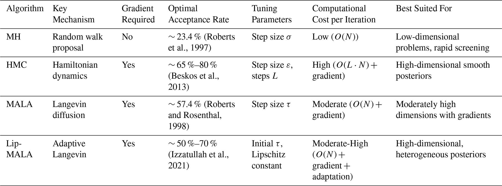
Table 1 summarizes the key characteristics, advantages, and limitations of the four algorithms, supported by theoretical and empirical studies from the literature.

Table 1 Comparative analysis of MCMC algorithms for seismic inversion.

3.5.1 Practical Implementation Notes

For our seismic inversion experiments, all algorithms were implemented with the following considerations:

1. Gradient Computation: The gradient $\mathrm{\nabla }\log p\left(m\right)=-\mathrm{\nabla }S\left(m\right)$ was computed analytically, ensuring computational efficiency.

2. Step Size Tuning: Each algorithm's step size parameter was tuned during a preliminary burn-in phase to achieve target acceptance rates.

3. Convergence Diagnostics: We employed diagnostics using Effective Sample Size (ESS) and multivariate ESS (Vats et al., 2019)

4. Computational Resources: All experiments were conducted on a workstation with Intel Core i9-10900K, 64GB RAM, without GPU acceleration. Execution times were measured as wall-clock time for fair comparison.

The following sections present application of these algorithms to synthetic and real seismic data, evaluating their performance in terms of accuracy, uncertainty quantification, and computational efficiency.

4 Results

4.1 Synthetic test

We test our algorithms using noise-free synthetic seismic traces that were obtained from real data of V_p, V_s and ρ for which synthetic seismic traces were generated from the Eq. (28) for the angles θ₁=9°, θ₂=18.5° and θ₃=27.5° and these synthetic seismic traces will be our observed data. We ran the sampling algorithms described in Sect. 3, producing a large chain of realizations, starting from a prior model configuration corresponding to a low frequency model of V_p, V_s and ρ.

Figure 3 shows the objective function variation curves for the different sampling algorithms. Each iteration involves randomly perturbing the velocities and density of a subset of layers and recalculation of seismic traces. The vertical axis represents the objective function calculated using Eq. (5). The horizontal axis shows the number of steps in the Markov chain, each associated with an accepted or rejected perturbation of the velocity and density configuration. The first stage of the chain, associated with the initial configuration and large residues, is called the burn-in or warm-up stage. After subtracting the residuals, the model realizations of velocities and densities satisfactorily explain the seismic data within the data errors. This is called the sampling phase. Realizations produced during the sampling phase are treated as samples from the probability density.

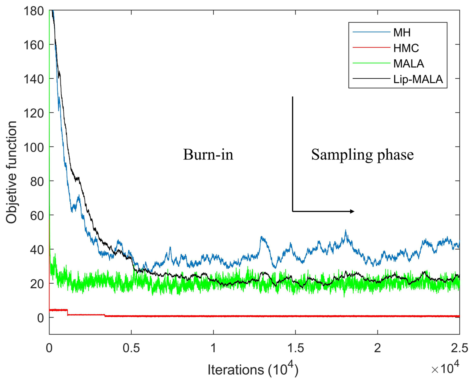
Figure 3 Progress with iterations in the MH (blue line), HMC (red line), MALA (green line) and Lip-MALA (black line) sampling algorithms for synthetic test.

The model settings were modified during the sampling phase, but remain within the probability function, as shown in Fig. 4. Figure 5 shows all realizations taken (gray area) in the chain sampling phase for the different algorithms tested in this work, all adjusting the observed seismic data and within the uncertainties of the data. These realizations indicate the features and variability of the velocities and density. Table 2 shows the statistical parameters of mean and standard deviation (SD) which we will compare then with the data obtained from the inference in the different algorithms used.

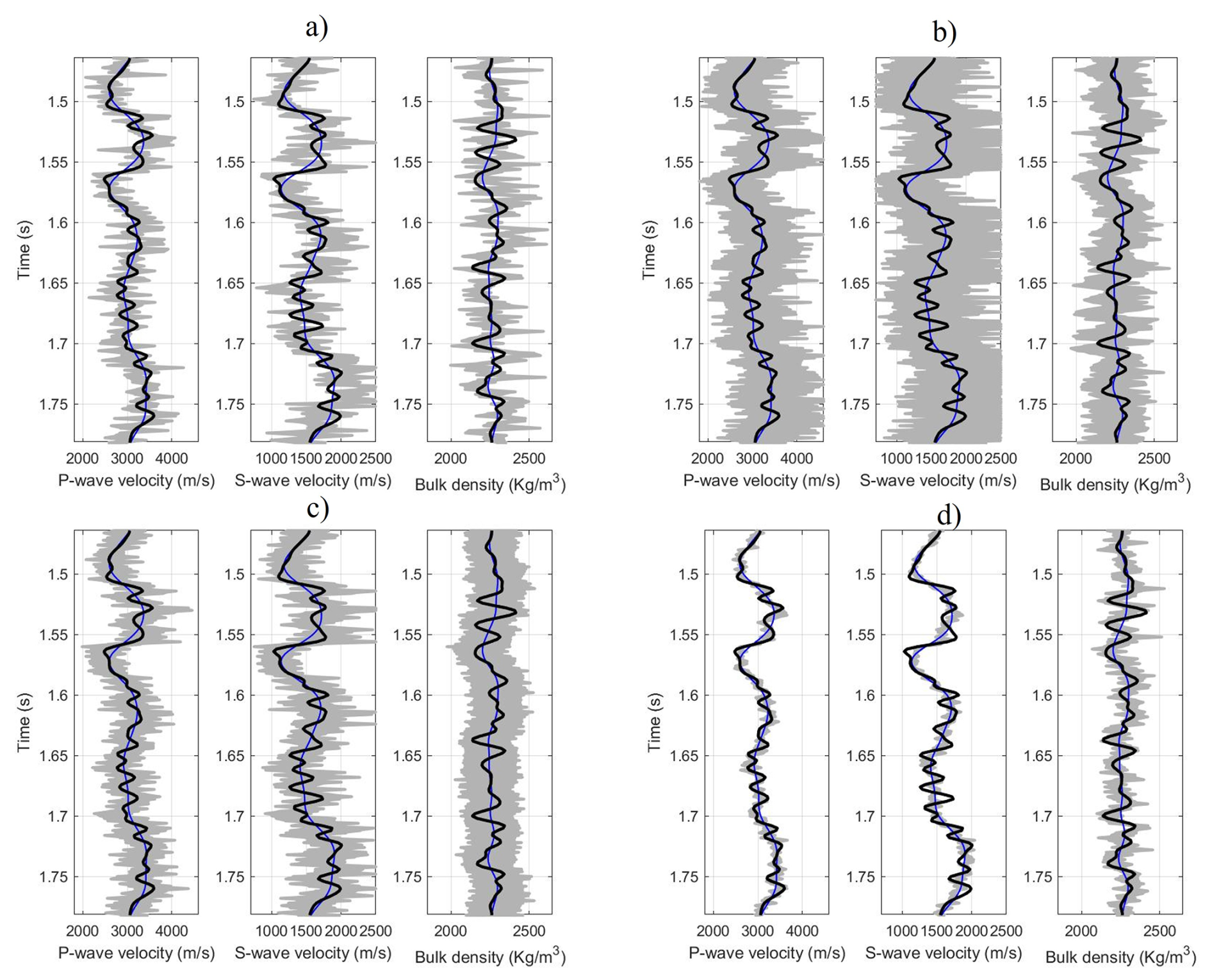
Figure 4 True data (black line), prior model (blue line), and accepted realizations of the model (gray) for the synthetic test where (a) MH, (b) HMC, (c) MALA, and (d) Lip-MALA.

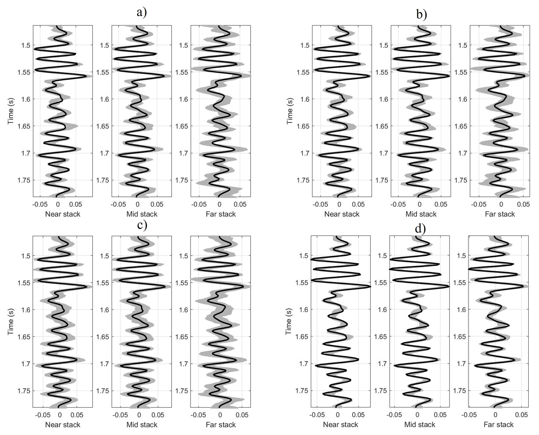
Figure 5 Observed seismic data (black line) and seismic traces obtained from the accepted model realizations (gray) for the synthetic test where (a) MH, (b) HMC, (c) MALA, and (d) Lip-MALA.

Table 2 Mean and Standard deviation of elastic parameters used in the synthetic test.

Our chain sampling phase yielded 10 000 realizations. From these realizations, we calculated the expected values and marginal probabilities of P-wave and S-wave velocities and density as a function of two-way reflection time. These calculations were based on averaging the model performances over the sampling phase. Figure 6 presents the marginal cumulative probability distributions for P and S wave velocities and density, as estimated by the inversion, along with the actual P and S wave velocities and density of the synthetic test. The figure demonstrates the successful prediction of the actual values for all tested algorithms, accurately identifying the main stratification characterized by high and low velocities and the corresponding high and low density.

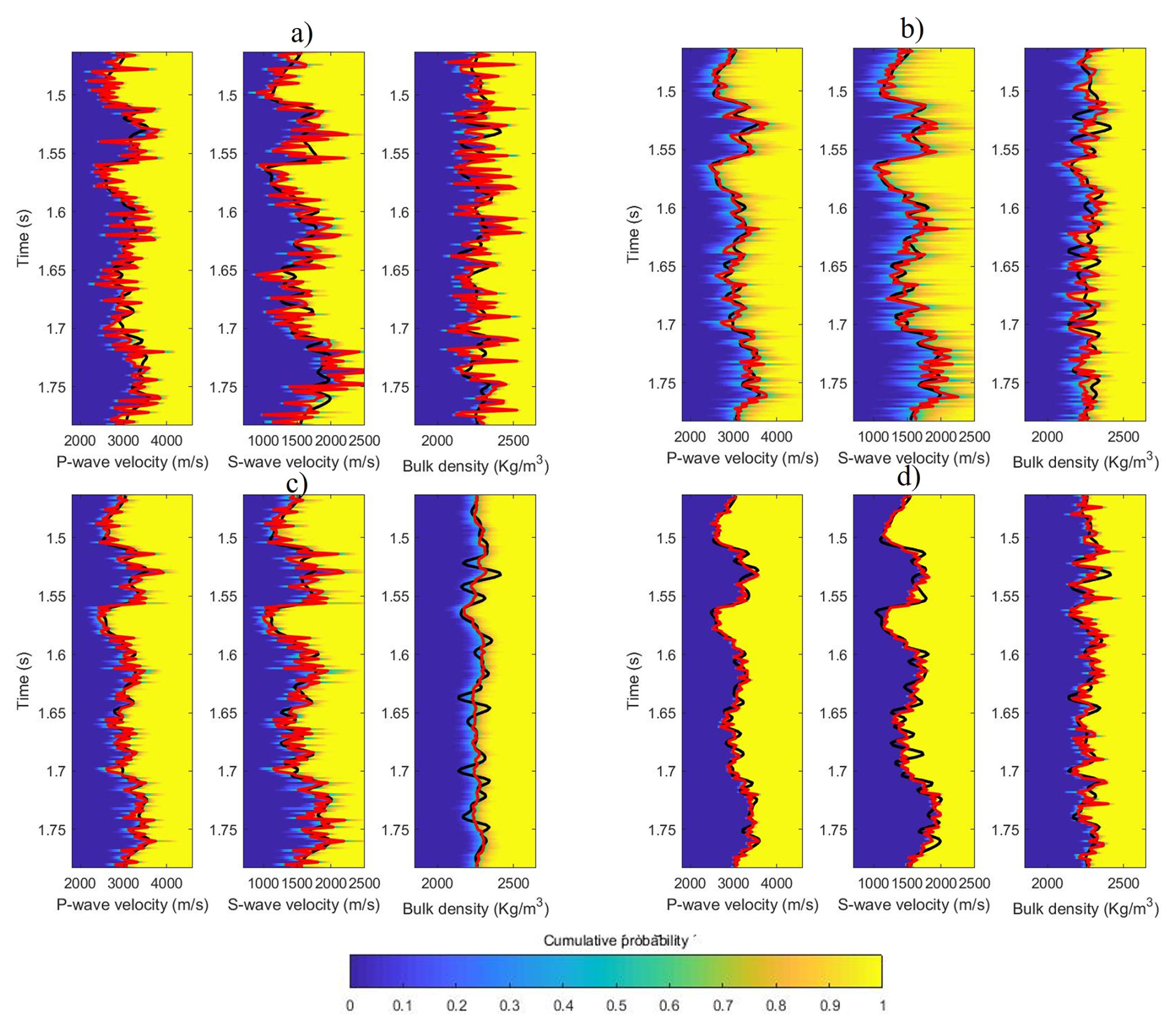
Figure 6 Marginal cumulative probability distributions (color map), true data (black line) and seismic inversion model result (red line) for the synthetic test where (a) MH, (b) HMC, (c) MALA, and (d) Lip-MALA.

Table 3 summarizes the performance of the different algorithms tested in predicting P-wave and S-wave velocities and density. The mean, Standard Deviation (SD), correlation, and Root Mean Squared Error (RMSE) are presented for each parameter.

Table 3 Statistical parameters for the results obtained for algorithms tested for the synthetic test.

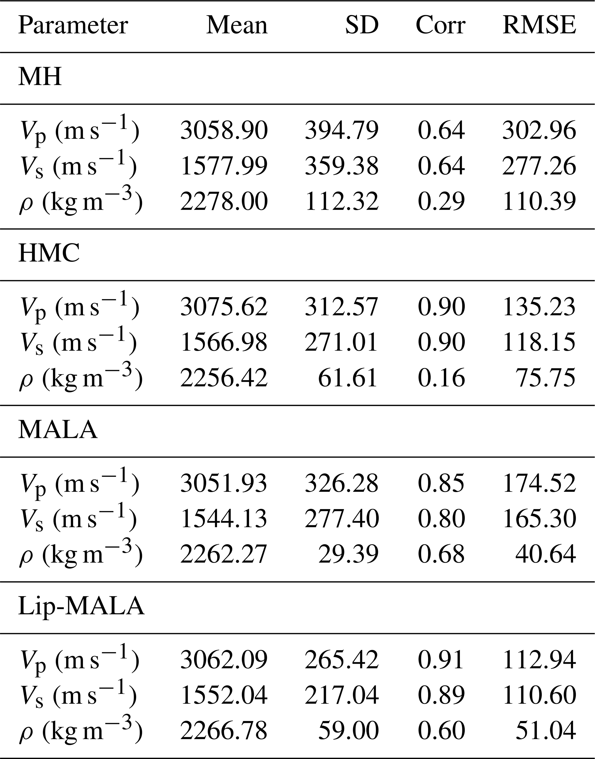
The mean and standard deviation values indicate that the predicted values are closely aligned with the true values. Regarding correlation, MH exhibits the lowest correlation for velocity prediction, while HMC achieves the highest. For density prediction, MH and HMC show correlations below 0.29, while MALA and Lip-MALA achieve correlations above 0.60.

In terms of RMSE, MH demonstrates the highest error for velocity prediction, while HMC achieves the lowest. For density prediction, MH and HMC exhibit errors above 75.75, while MALA and Lip-MALA maintain errors below 51.04.

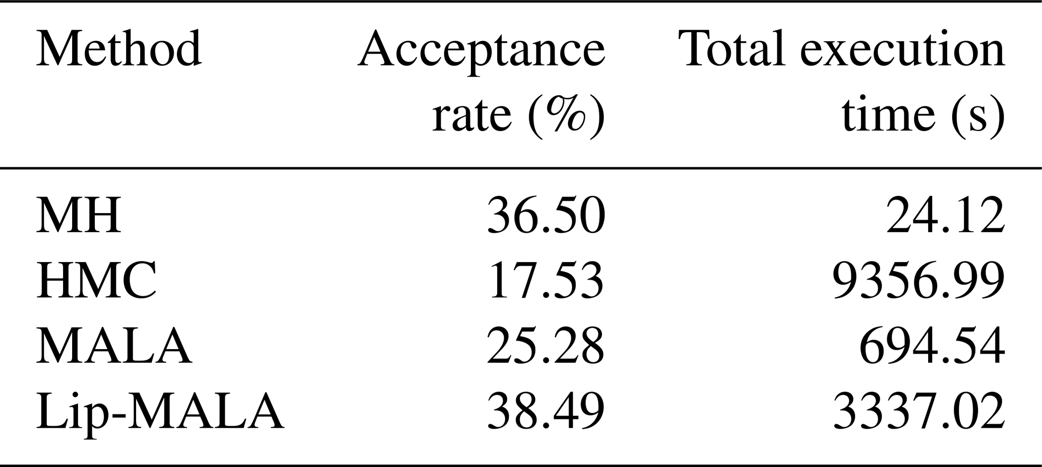
Table 4 presents various performance parameters, including acceptance rate and total execution time. Lip-MALA exhibits the highest acceptance rate, while HMC exhibits the lowest. Conversely, MH boasts the lowest total execution time, while HMC demonstrates the highest.

Table 4 Other parameters for synthetic test.

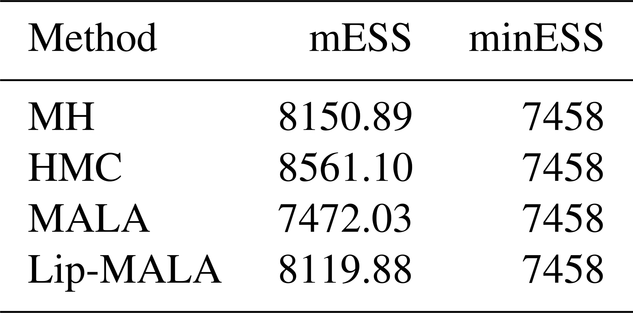
Finally, the convergence of the samples was analyzed a posteriori of the unknown parameters (seismic data parameters) m obtained from the different algorithms used. The multivariate effective sample size (mESS) statistic was used. The mESS is a measure that determines the size of an independent and identically distributed sample with the same covariance structure as the sample obtained from an MCMC method for the multivariate case- If we want to know if the chain converges by we can calculate minimum effective sample size (minESS) so that if mESS > minESS we say that the chain converges, if the reader is recommended to review Vats et al. (2019) to delve deeper into the convergence test used in this work. Table 5 shows the summary of mESS and minESS obtained for each method.

Table 5 Convergence test for synthetic data.

4.2 Application to real data

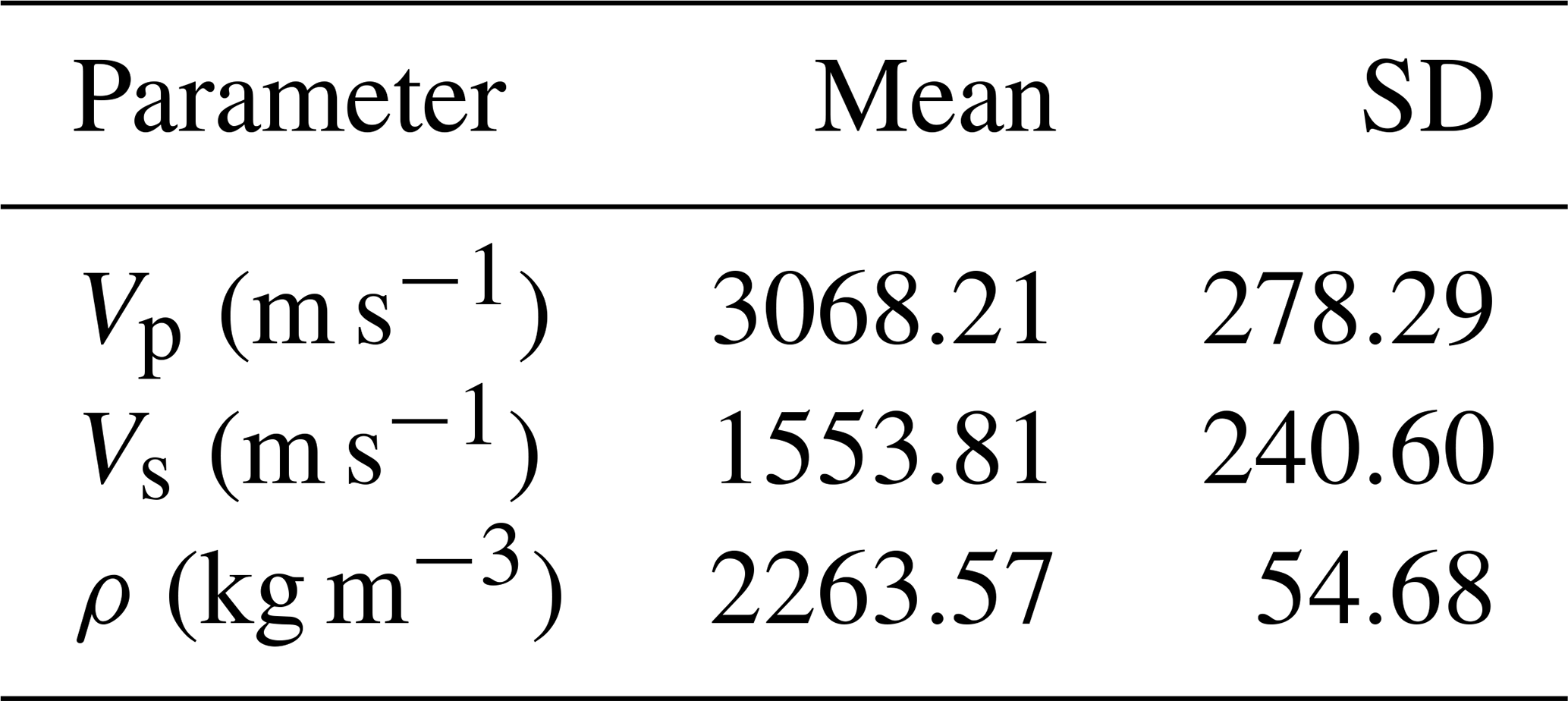
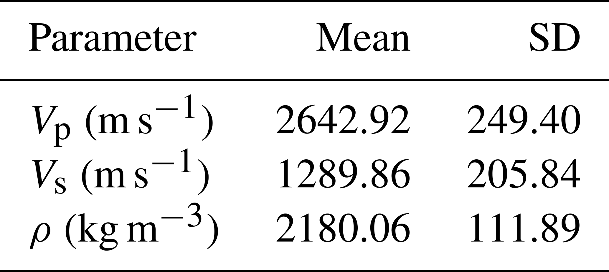
To demonstrate the effectiveness of the algorithms, we applied them to a real dataset of an oil field in eastern Venezuela. The site is located in a formation dominated by clastic rocks, a type of sedimentary rock characterized by alternating layers of sand and shale. The fluids in the pore spaces of these rocks are brine water and oil, without gas. As a preliminary step, we upscaled the P-wave and S-wave velocities obtained from well log data to the corresponding seismic scale using a bandpass filter. This process ensures that the velocity data is consistent with the frequency range of seismic waves. Table 6 presents the descriptive statistics, including mean and standard deviation (SD), for the real data. These values will serve as a baseline for comparison with the results obtained from the inference procedures employed by the various algorithms under consideration.

Table 6 Mean and Standard deviation of elastic parameters used for real data.

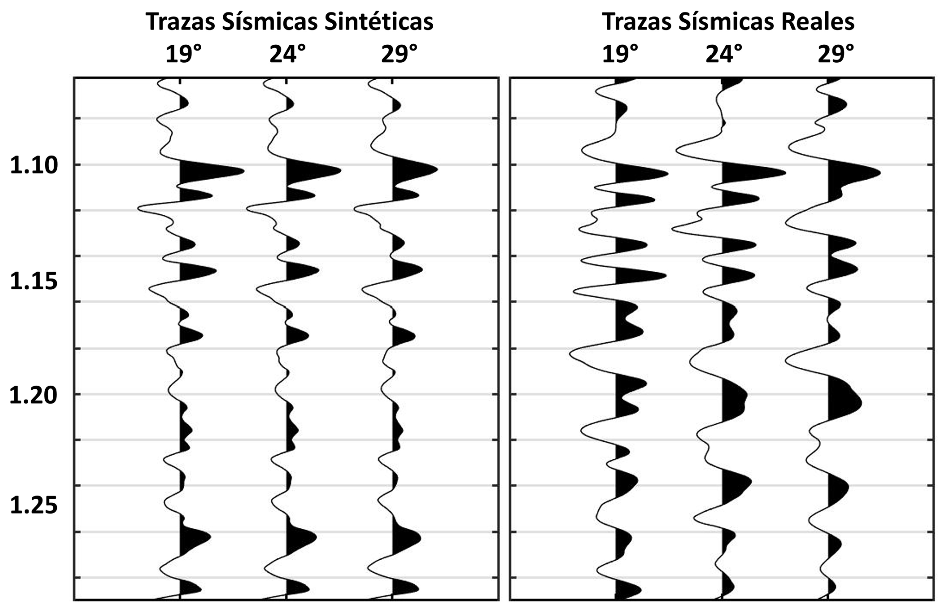
The seismic traces were obtained from partial stacks for the angles θ₁=19°, θ₂=24°, and θ₃=29°. Utilizing V_p, V_s and ρ logs in seismic scale and wavelets were extracted from the partial stacked seismic data using the frequency content of the data, the synthetic trace was generated using Eq. (13). The synthetic trace obtained was correlated with observed traces for seismic well tie (see Fig. 7) obtaining a correlation value of 0.55. The sampling algorithms described in Sect. 3 were implemented, generating a large chain of realizations starting from a prior model configuration corresponding to a low-frequency model of V_p, V_s and ρ.

Figure 7 Seismic well tie for real data used.

As depicted in Fig. 8, the objective function variation curves for each sampling algorithm are presented. During each iteration, a subset of layers undergoes a random perturbation of their velocities and density, followed by a recalculation of the seismic trace. The objective function, calculated using Eq. (5), is represented on the vertical axis, while the horizontal axis represents the number of steps in the Markov chain. Each step corresponds to an accepted or rejected perturbation of the velocities and density configuration.

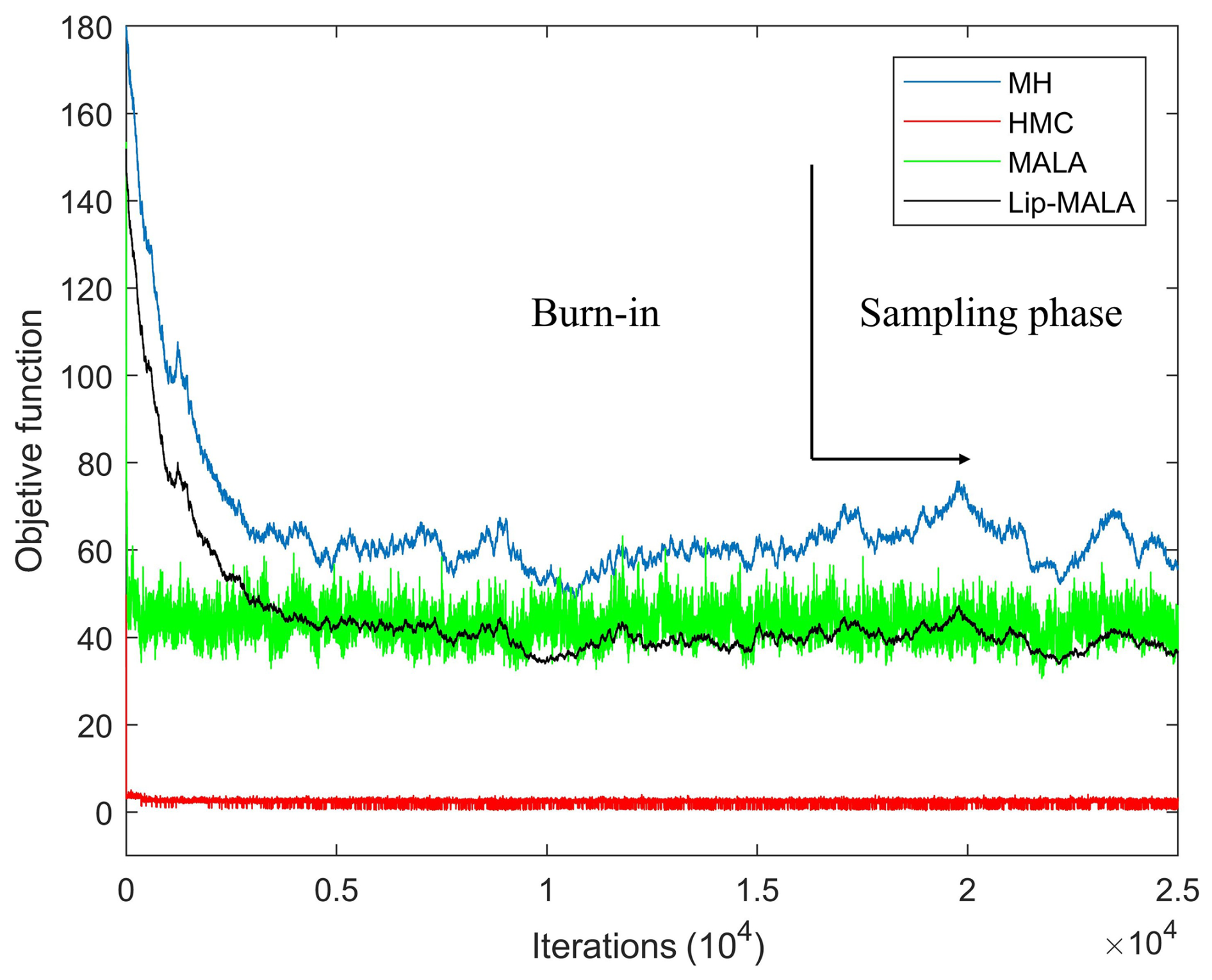
Figure 8 Progress with iterations in the MH (blue line), HMC (red line), MALA (green line) and Lip-MALA (black line) sampling algorithms for real data.

The model settings were adjusted during the sampling phase, ensuring they remained within the probability function (Fig. 9). Figure 10 illustrates all realizations sampled (gray area) in the chain sampling phase for the various algorithms tested in this study, all of which align with the observed seismic data and fall within the data's uncertainty bounds. These realizations highlight the characteristics and variability of the velocities and density.

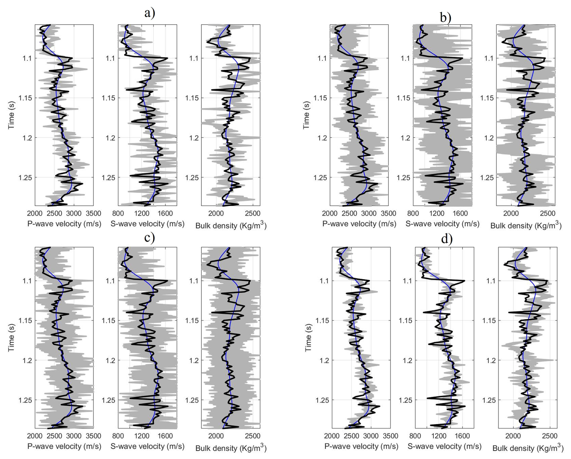
Figure 9 True data (black line), prior model (blue line), and accepted realizations of the model (gray) for real data where (a) MH, (b) HMC, (c) MALA, and (d) Lip-MALA.

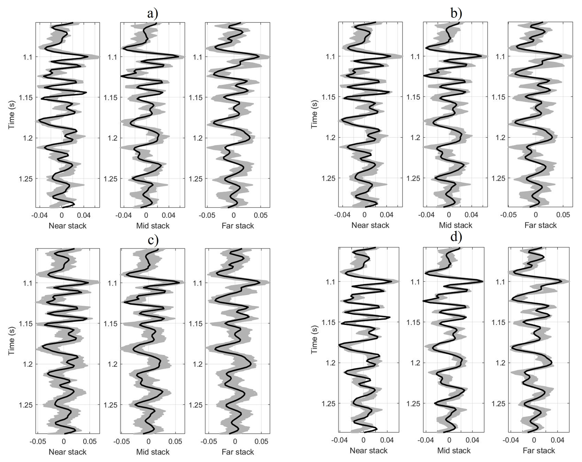
Figure 10 Observed seismic data (black line) and seismic traces obtained from the accepted model realizations (gray) for real data where (a) MH, (b) HMC, (c) MALA, and (d) Lip-MALA.

Employing a chain sampling scheme, we generated 9000 realizations from which we extracted the expected values and marginal probabilities of P-wave and S-wave velocities and density, all as functions of two-way reflection time. These calculations were derived by averaging the model performances across the sampling phase. Figure 11 depicts the marginal cumulative probability distributions for P and S wave velocities and density, as inferred from the inversion process, alongside the actual P and S wave velocities and density of the synthetic test.

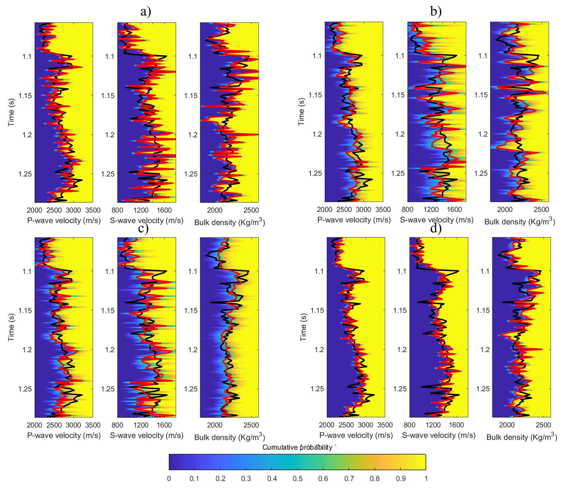
Figure 11 Marginal cumulative probability distributions (color map), true data (black line) and seismic inversion model result (red line) for real data where (a) MH, (b) HMC, (c) MALA, and (d) Lip-MALA.

Table 7 summarizes the performance of the tested algorithms in predicting P-wave and S-wave velocities and density. The mean, Standard Deviation (SD), correlation, and Root Mean Squared Error (RMSE) are presented for each parameter. The predicted values closely align with the true values as evidenced by the mean and standard deviation values. MH exhibits the lowest correlation for velocity prediction, while Lip-MALA achieves the highest. For density prediction, MH and HMC show correlations below 0.28, while MALA and Lip-MALA achieve correlations above 0.48. MH demonstrates the highest error for velocity prediction, while Lip-MALA achieves the lowest. For density prediction, MH and HMC exhibit errors above 151.41, while MALA and Lip-MALA maintain errors below 122.22.

Table 7 Statistical parameters for the results obtained for algorithms tested for real data.

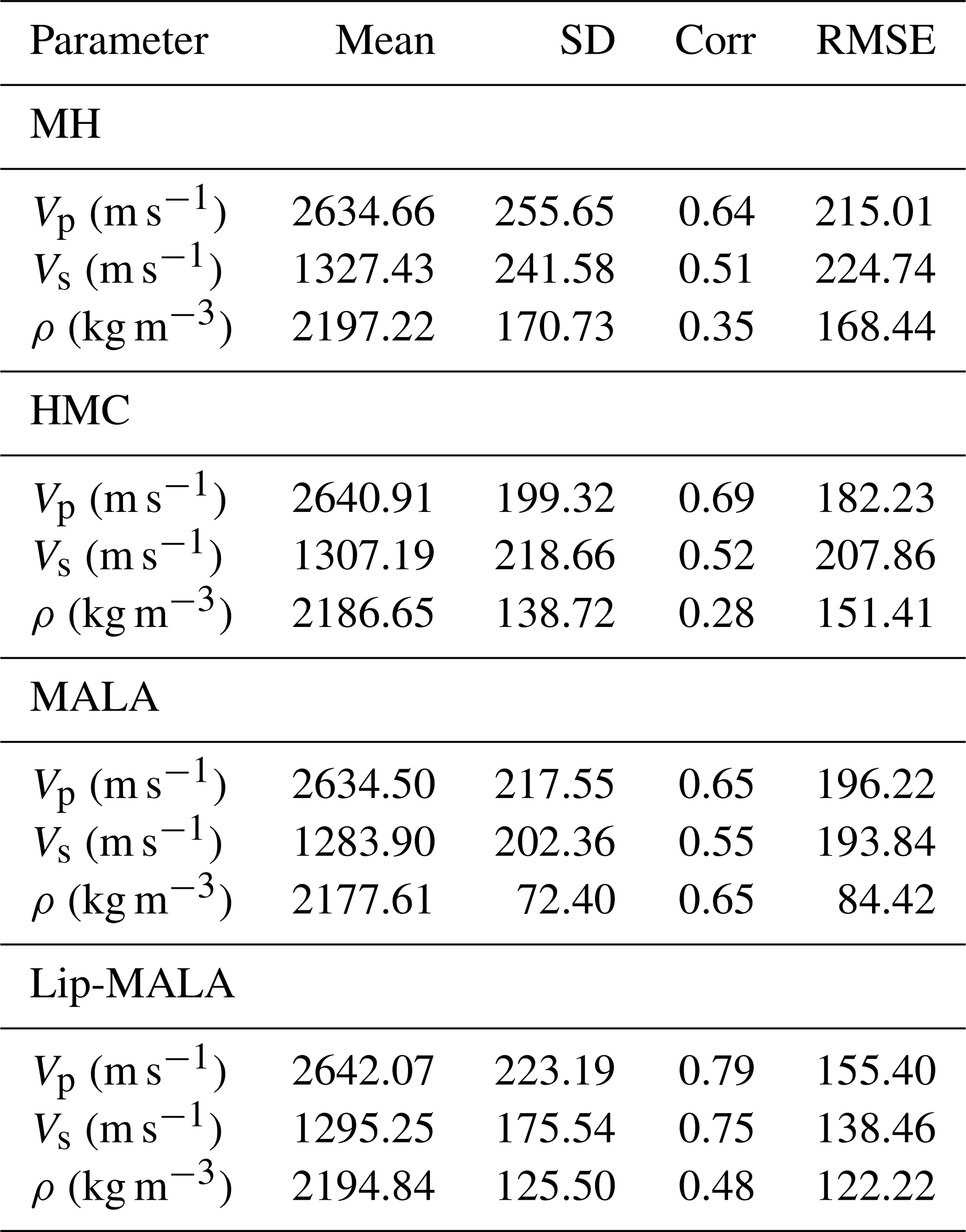
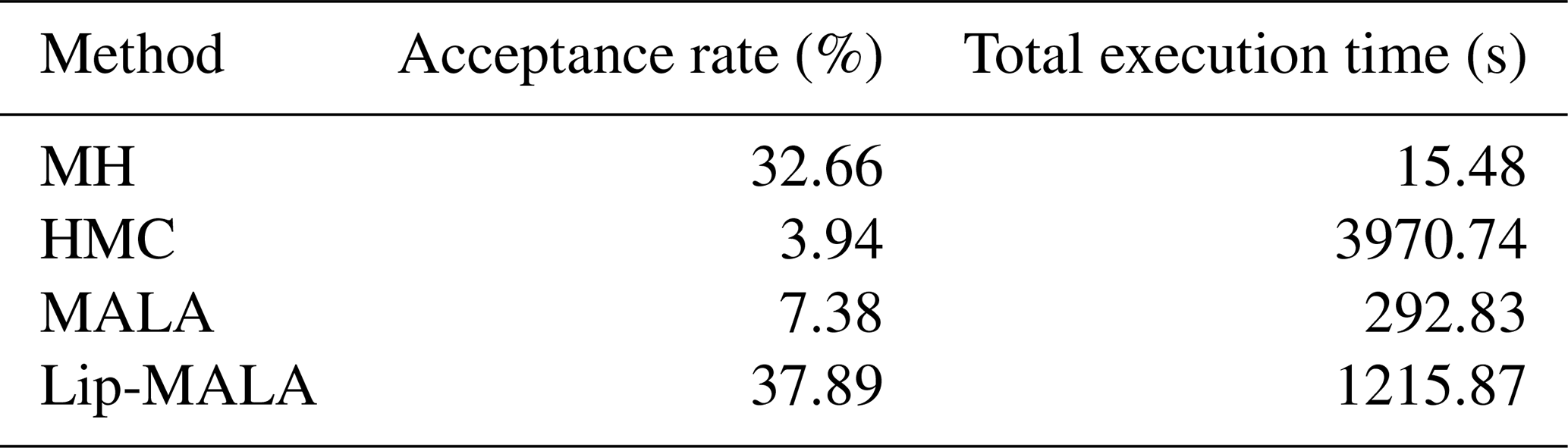
Table 8 presents various performance parameters, including acceptance rate and total execution time. Lip-MALA exhibits the highest acceptance rate, while HMC exhibits the lowest. Conversely, MH boasts the lowest total execution time, while HMC demonstrates the highest.

Table 8 Other parameters for real data.

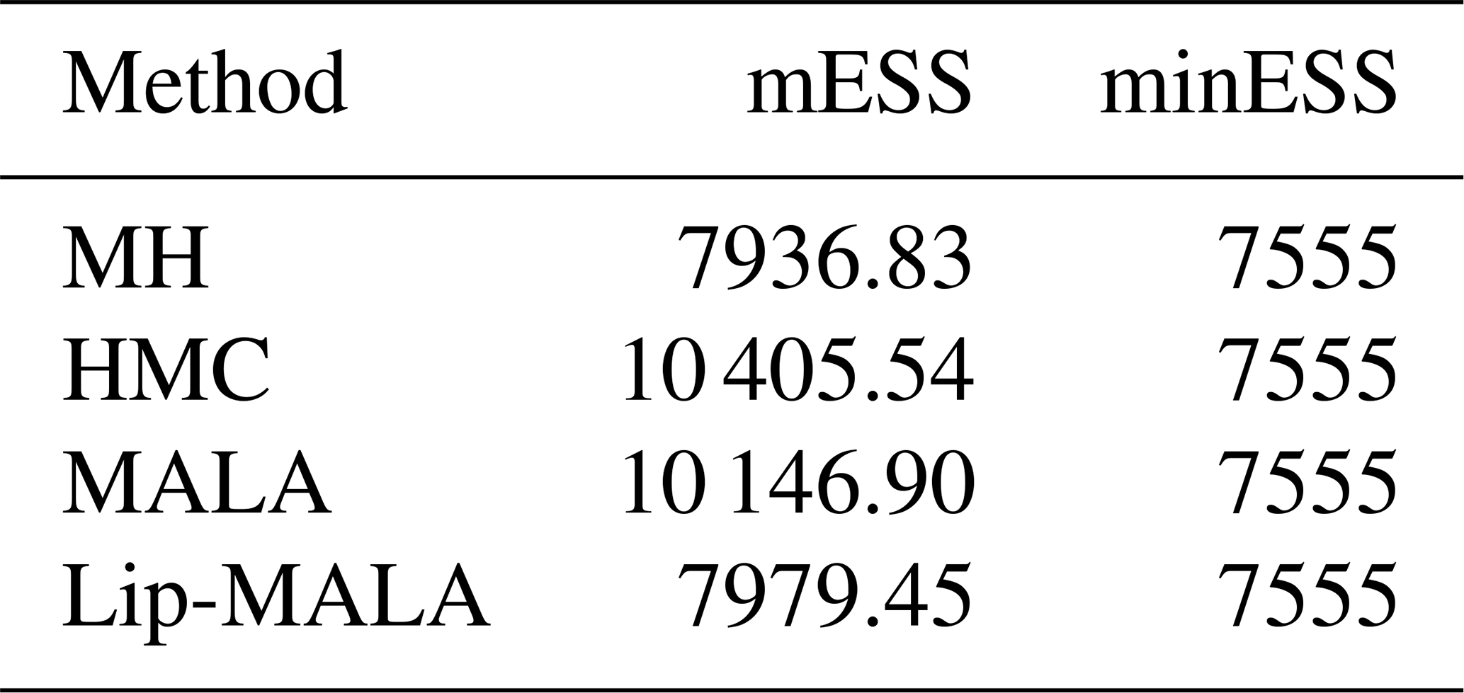
And a final step, as in the synthetic data, was to test the convergence of the chains, this study employed a posteriori analysis to assess the convergence of samples obtained for the unknown seismic data parameters (denoted by m) using various algorithms. The multivariate effective sample size (mESS) statistic served as the convergence metric. The mESS quantifies the equivalent size of an independent and identically distributed (iid) sample possessing the same covariance structure as the sample generated by a Markov Chain Monte Carlo (MCMC) method in the multivariate case.

To formally determine chain convergence, a minimum effective sample size (minESS) threshold can be established. If the mESS value surpasses the minESS threshold, convergence is achieved. For a more in-depth exploration of the convergence test employed in this work, readers are referred to Vats et al. (2019). Table 9 summarizes the mESS and minESS values obtained for each method.

Table 9 Convergence test for real data.

Table 10 Posterior standard deviations (2D real data).

4.3 Two-dimensional test with real data

In line with the main objective of this study, which is to comparatively evaluate the performance of different MCMC algorithms applied to prestack seismic inversion in geological contexts of varying complexity, this section includes an additional test using real data in a two-dimensional setting. This extension allows us to validate the scalability and robustness of the methods beyond idealized one-dimensional cases, providing evidence of their practical applicability in environments with greater structural and lithological heterogeneity, typical of exploration in real reservoirs.

The study area corresponds to a sector of the Eastern Basin of Venezuela, characterized by clastic lithology with alternating sandstones and shales. The seismic data used was acquired using conventional reflection techniques and subsequently reprocessed to generate prestack gathers organized by incidence angle. Three partial stacks were selected, corresponding to central angles of approximately 19, 24, and 29°, and used in the inverse process.

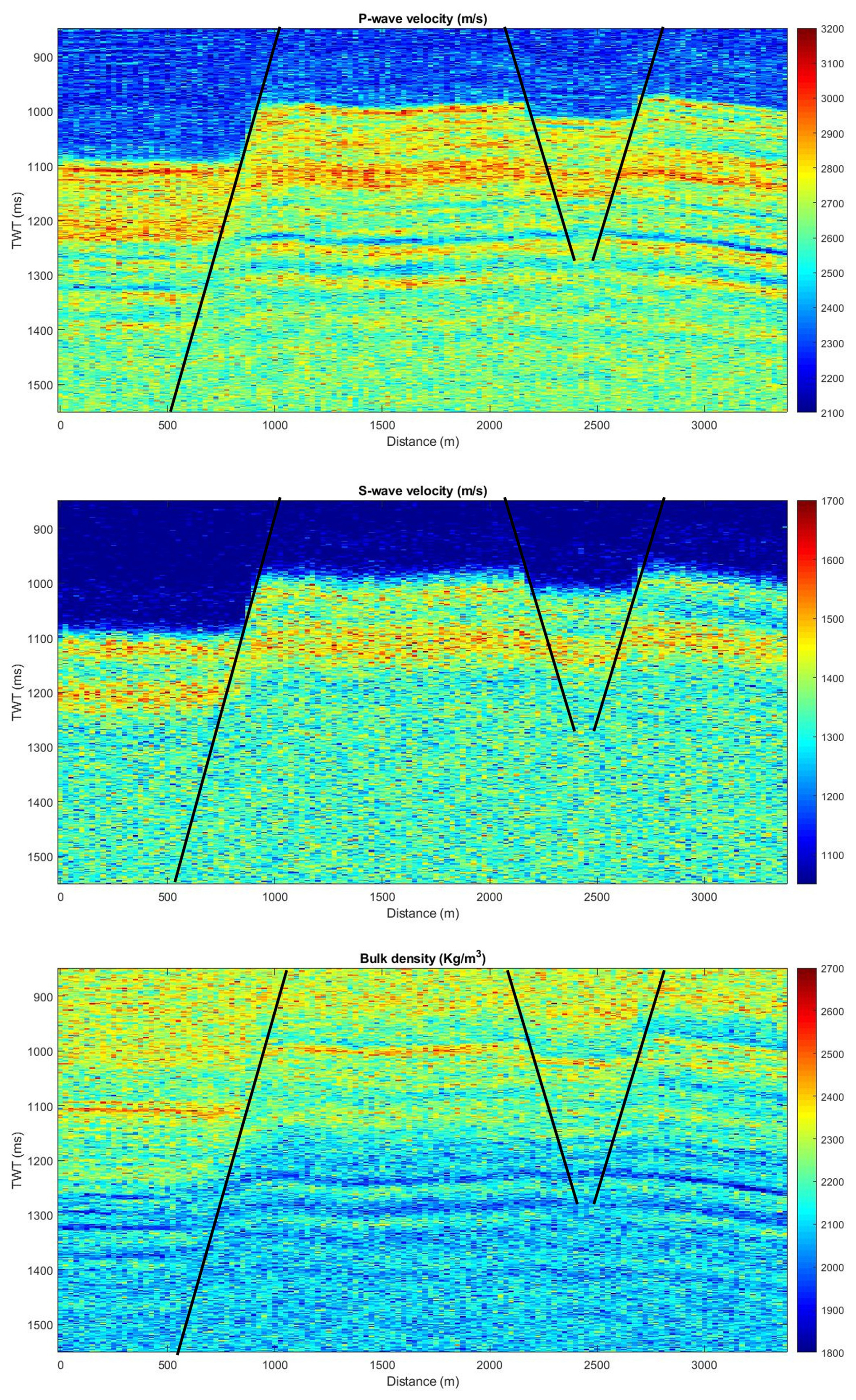
The two-dimensional inversion grid was designed with a vertical resolution of 351 samples, corresponding to the two-way time axis from 850 to 1550 ms, and a horizontal extent of 136 cells from 0 to 340 m. Three fundamental elastic parameters were considered: V_p, V_s and ρ. The prior model was built by integrating the structural interpretation of horizons and faults obtained from seismic data, together with low-frequency interpolation of the elastic properties V_p, V_s and ρ. derived from the well logs available in the study area. This approach allowed the establishment of a consistent geological model that served as an initial reference for the Bayesian inversion process.

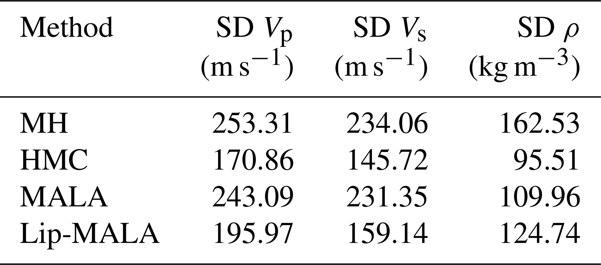
The four MCMC sampling algorithms analyzed were applied in 1D: MH, HMC, MALA, and Lip-MALA. The resulting realizations were used to calculate the posterior marginal distributions for each parameter, as well as their summary statistics (mean and standard deviation, Table 10).

Quantitative analysis of the Figs. 12 to 15 reveals important differences between the algorithms. The HMC method presents the lowest standard deviations for all three parameters, indicating greater accuracy and lower uncertainty in the estimation, although at the cost of higher computational costs. MALA and Lip-MALA also offer robust results, with Lip-MALA demonstrating a better compromise between accuracy and computational efficiency, especially in density estimation. In contrast, the MH algorithm shows the greatest uncertainties, confirming its limitations in contexts of higher dimensionality and complexity.

Figure 12 Inverted models of V_p, V_s and ρ obtained using the MH algorithm.

Figure 13 Inverted models of V_p, V_s and ρ obtained using the HMC algorithm.

Figure 14 Inverted models of V_p, V_s and ρ obtained using the MALA algorithm.

Figure 15 Inverted models of V_p, V_s and ρ obtained using the Lip-MALA algorithm.

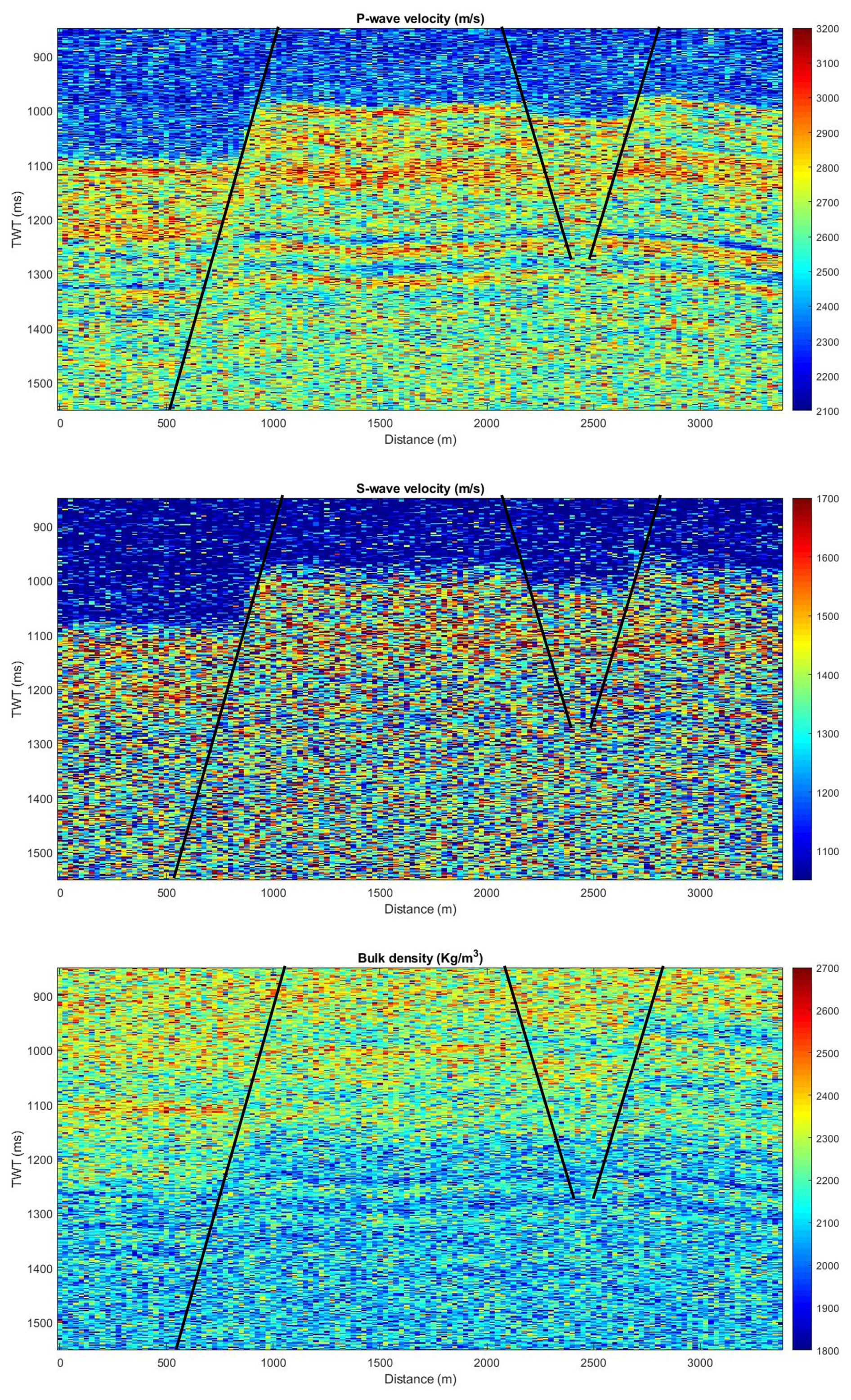
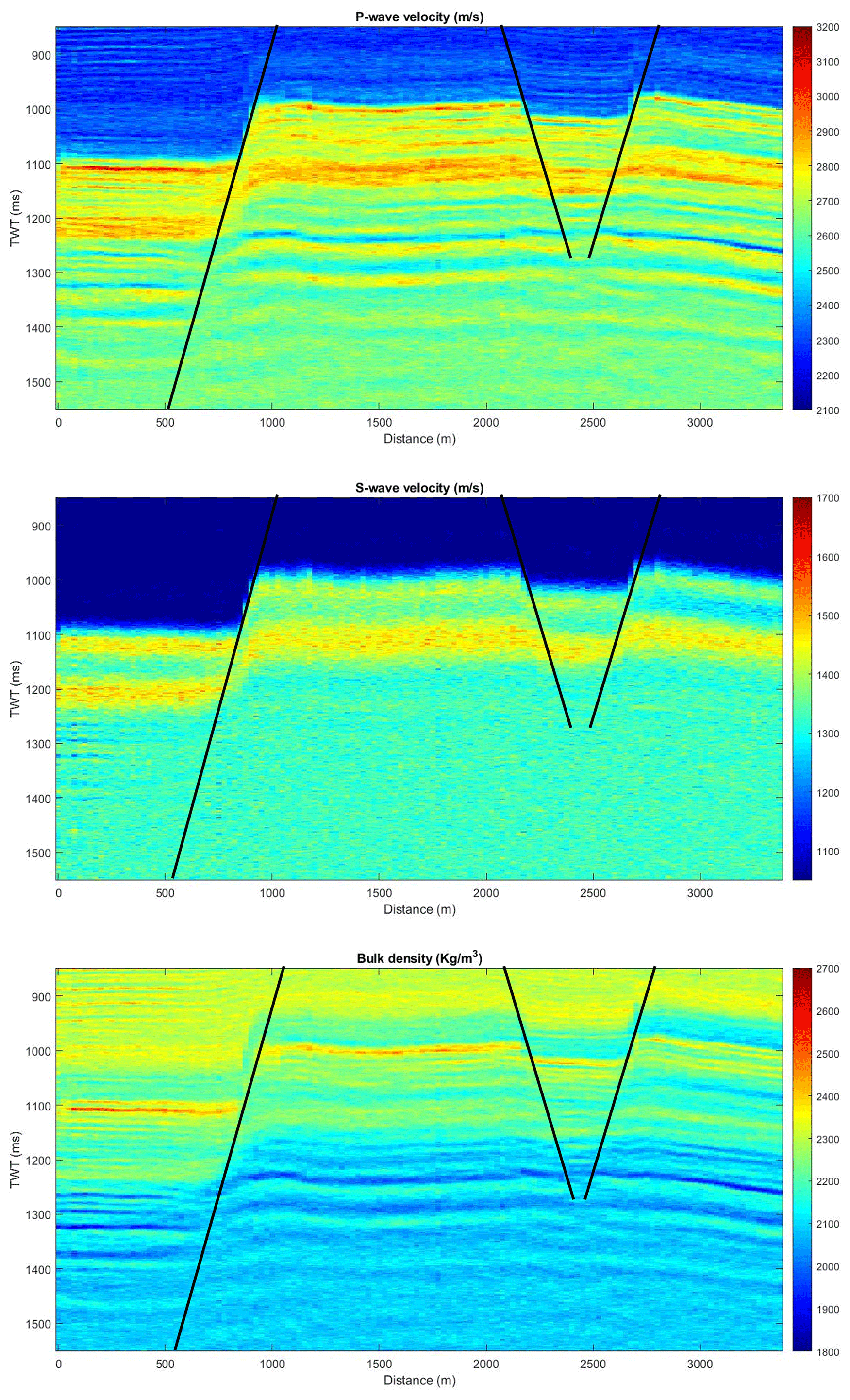
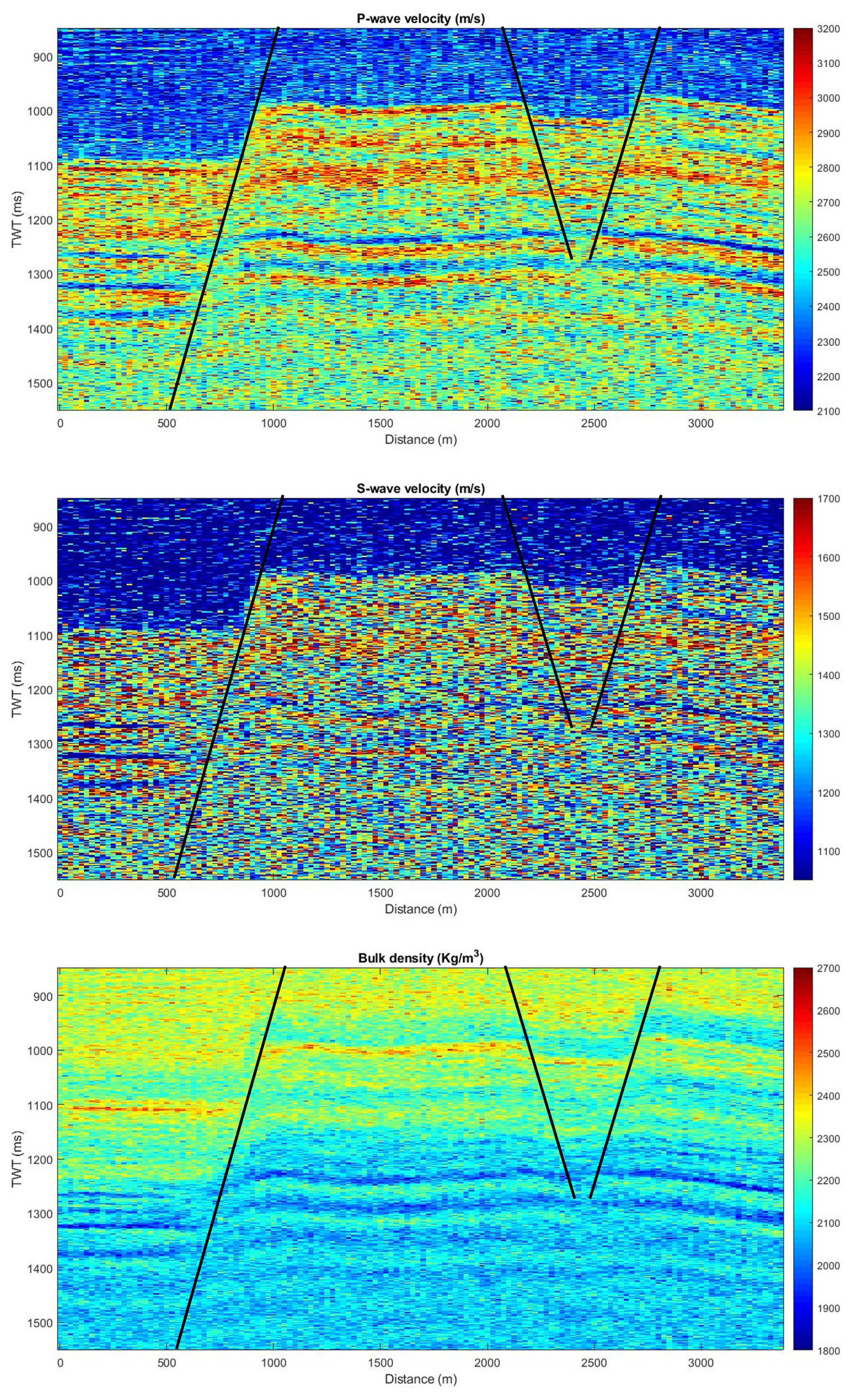
From an applied perspective, these results are relevant for choosing the most appropriate method in exploratory contexts. In situations where high accuracy is required and sufficient computational resources are available, HMC may be the preferred option. On the other hand, in scenarios where computational time is a constraint, methods such as Lip-MALA offer an efficient and stable alternative. Density (ρ) remains the most challenging parameter to accurately recover, especially for MH and HMC, which is consistent with the results obtained in the one-dimensional case.

Finally, the incorporation of this two-dimensional test with real data demonstrates the practical applicability of the evaluated algorithms, not only under controlled conditions but also in situations representative of real-world geology. Furthermore, it reinforces the validity of the study's overall conclusions by confirming that gradient-based algorithms are more appropriate for complex inverse scenarios, and that algorithm selection must consider both the level of uncertainty and computational cost.

5 Discussion

This study presents a comparative analysis of Markov Chain Monte Carlo (MCMC) methods for estimating elastic properties from seismic amplitudes. We demonstrate the application of these methods in a field case, employing the following assumptions: (1) a one-dimensional reservoir model represented by stacked seismic traces, (2) seismic data simulation using the small reflectivity approximation, and (3) the Aki-Richards equation for weak contrast to establish the relationship between seismic data and elastic parameters. Notably, the proposed general formulation transcends these assumptions, allowing for the integration of more sophisticated seismic simulation techniques and comprehensive petrophysical models within a similar framework. Why does Lip-MALA yield smaller errors in the theoretical (1D) test while HMC performs better in the two-dimensional real case? In our experiments, two factors explain this: (i) the evaluation metric and (ii) the dimensionality/structure of the posterior.

• i.

  Metric. In 1D (synthetic and real), we compared primarily RMSE along the trace; Lip-MALA, by enforcing a Lipschitz-based step control, stabilizes local moves and reduces pointwise error (RMSE) in V_p and V_s. In 2D, we mainly reported posterior SD per parameter; HMC, via long Hamiltonian trajectories, explores connected valleys of the posterior more efficiently and achieves lower global uncertainty (SD), even if RMSE 2D is not emphasized in the main text.

• ii.

  Dimensionality/heterogeneity. In real 2D, lateral couplings and heterogeneity induce a rough/multimodal posterior; HMC traverses basins more effectively than local Lip-MALA steps, reducing posterior variance.

  The four methods studied demonstrate acceptable performance, but in-depth analysis reveals notable differences:

  • –

    Velocity estimation: In both the synthetic and real-world scenarios, methods that incorporate gradient calculations (HMC, MALA, and Lip-MALA) outperform MH in estimating velocities.

  • –

    Density estimation: Density estimation proves to be the most challenging parameter, with MH and HMC exhibiting unsatisfactory results. However, MALA and Lip-MALA showcase more promising performance.

  • –

    Execution time: A significant difference emerges in execution time between methods. MH and MALA exhibit shorter execution times compared to HMC and Lip-MALA, which are considerably more time-consuming.

A natural progression of this research would be to invert prestack seismic data to extract additional elastic parameters and reservoir properties, revealing a more comprehensive subsurface understanding. Similarly, incorporating well log conditioning into the model holds promise, as it could enhance vertical resolution near wells and guarantee that the model aligns with well data at drilling locations.

From an applied perspective, the results obtained in this study are relevant for decision-making in real-world exploration settings. For example, in frontier areas with poor well control, the MH algorithm could be used as a rapid evaluation tool due to its low computational cost, albeit with accuracy limitations. In contrast, methods such as HMC or Lip-MALA would be more suitable for mature fields where higher fidelity in estimating elastic properties is required, despite their greater computational demand. The choice of algorithm should be guided not only by statistical metrics but also by the specific requirements of the geophysical project, the geological setting, and the time and resource constraints available.

The results obtained in this work show consistency with previous research. For example, Gebraad et al. (2020) highlights the effectiveness of the HMC algorithm in full-waveform elastic inversion problems, particularly due to its ability to efficiently explore the posterior space. However, unlike their FWI-oriented approach, our AVO inversion results indicate that Lip-MALA achieves a better balance between accuracy and computational cost, particularly in density estimation, which is crucial in clastic media with gradual transitions. Similarly, Izzatullah et al. (2021) demonstrated that Langevin dynamics-based methods, such as MALA and its adaptive variants, are more efficient in high-dimensional spaces, which is reflected in our study by better definition of lithological boundaries in inverted images. These parallels confirm that Langevin-derived methods are viable and robust options in real-world seismic scenarios where efficiency and stability are practical priorities.

Although the HMC algorithm presents significantly longer runtimes, these may be acceptable within a seismic interpretation workflow that includes validation and multidisciplinary analysis phases. In contexts where the inversion must be performed in near-real time, such as during well drilling (geosteering), methods such as MH or MALA may be more appropriate despite their lower resolution. Therefore, computation time should not be evaluated in isolation, but rather based on operational priorities, available computational resources, and the criticality of the information to be estimated at each stage of the geophysical project.

6 Conclusions

This study compares various pre-stack inversion methods under an MCMC framework for the estimation of elastic parameters. We invert pre-stacked seismic data to infer velocities (V_p and V_s) and density (ρ), which are linked to the seismic data via the Aki-Richards equation. All methods employed effectively handle the inherent uncertainties associated with seismic and elastic data.

The proposed algorithms allow estimating several important aspects of the posterior distribution, such as the means and standard deviations of the posterior parameters. We rigorously validated the algorithms by measuring the quality of the MCMC sample through correlations, plotting the objective function, seismic traces and estimating the RMSE.

The four methods evaluated in this study exhibit acceptable performance overall, but a closer examination reveals notable differences in their specific capabilities. Velocity estimation: In both the simulated and real-world scenarios, methods that leverage gradient calculations (HMC, MALA, and Lip-MALA) demonstrate superior performance in estimating velocities compared to MH. Density estimation: Density estimation poses the most significant challenge, with MH and HMC exhibiting unsatisfactory results. However, MALA and Lip-MALA demonstrate more promising performance in this area. Execution time: A clear distinction emerges in execution time between the methods. MH and MALA exhibit significantly shorter execution times compared to HMC and Lip-MALA, which are considerably more time-consuming.

Furthermore, the results of the two-dimensional test with real data showed that in situations where high accuracy is required and sufficient computational resources are available, HMC may be the preferred option. On the other hand, in scenarios where computational time is a constraint, methods such as Lip-MALA offer an efficient and stable alternative. This validation in a context closer to real geology strengthens the study's conclusions. The choice of algorithm must consider not only statistical metrics but also the geophysical context, resource availability, and project purpose. In summary we have:

• Balance runtime vs accuracy: HMC yields lower SD at higher cost; Lip-MALA provides strong local accuracy efficiently.

• Choose metrics deliberately: report both RMSE (fit) and SD (uncertainty) to avoid metric-induced contradictions.

• Use HMC for 2D (and higher) problems to reduce global posterior SD and traverse multi-basin landscapes.

• Use MALA/Lip-MALA to stabilize density estimation and reduce pointwise errors.

• Use Lip-MALA when local accuracy (lower RMSE) in VP/VS is prioritized on 1D settings.