Inferring the role of Interdecadal Pacific Oscillation phase on tropical-extratropical teleconnection dependencies

Regime dependencies and Granger causal relationships between tropical and extratropical teleconnections are inferred using Bayesian structure learning. Using ERA5 data, an examination of the differences between the learned graphical structures during particular phases of the Interdecadal Pacific Oscillation (IPO) are used to infer the role of the background state on interactions between the major climate teleconnections. These relationships present a clear regime dependency on the phase of IPO. In the positive phase, IPO autocorrelations are weak whereas Indian Ocean Dipole (IOD) and El Niño Southern Oscillation (ENSO) autocorrelations and the influence of the Madden Julian Oscillation (MJO) are indicative of an enhanced Walker circulation. In contrast, during the negative phase, IPO autocorrelations are strongest with evidence of an enhanced role for extratropical teleconnections on the tropics. Exclusion of MJO removes important tropical-extratropical influences while increasing posterior edge weights between ENSO, the IPO and IOD. Our analysis reveals the dependence of the ENSO autocorrelation on the phase of the background IPO state, and the role of the MJO as being key to link the extratropical tropospheric modes Pacific North American and North Atlantic Oscillation (PNA, NAO) and equatorial surface ocean temperatures (IOD, ENSO) and as a consequence convection.

1 Introduction

The complexity of the climate system is most evident in the interactions between the respective internal modes of variability, otherwise known as teleconnections, modes that are distinct in both geographical location and timescale. Whereas internal variability occurs on timescales from synoptic to inter-annual, the longer time- and larger spatial-scale multi-decadal modes act as background states, most notable of which are the Interdecadal Pacific Oscillation (IPO) and Atlantic Multi-decadal Oscillation (AMO). The extent to which these low frequency background states impose regime dependencies on the shorter timescale internal modes, and therefore their intrinsic predictability, remains largely an open question. Quantifying (Granger) causal relationships from reanalyses or data from dynamic general circulation models (GCMs) is challenging due to the dimensionality and large sample sizes required to determine accurate statistical measures from often non-stationary timeseries. Recent work by the authors (Harries and O'Kane, 2021; O'Kane et al., 2024) has shown that the current generation of GCMs often exhibit large systematic biases in representing autocorrelations and dependencies in graphical representations of their associated structural causal models. The ability to quantify model biases and their uncertainties in relation to observational products from a causal perspective is key to determining not only the source of any given model error but to enhancing our understanding of the climate system thereby aiding the development of better predictive systems.

In this study we seek to quantify differences in the inferred dynamic Bayesian network structures describing interactions between the major modes of tropical ocean and extratropical atmospheric variability for alternative phases of the dominant background state of the Pacific Ocean over multidecadal timescales. To this end, we examine extensively studied large scale modes of climate variability including an index of the IPO during representative phases of the IPO. The IPO (Power and Coleman, 2006; Meehl et al., 2010; Dong and Dai, 2015; Heidemann et al., 2023) characterizes low frequency sea surface temperature (SST) variability on decadal timescales over the entire Pacific basin, incorporating variations due to the El Niño Southern Oscillation (ENSO), the North Pacific Decadal oscillation (PDO) (Mantua et al., 1997), and the South Pacific Decadal Oscillation (SPDO) (Chen and Wallace, 2015). The IPO, as characterized by the Tripolar Index (TPI) of Henley et al. (2015), exhibits a distinct “tripole” pattern of SST spanning the Pacific Ocean from the Northern Hemisphere subtropics to the Southern Hemisphere subtropics. Over the decades covered by reanalysis data sets, debate on the mechanisms driving substantive variations in the phase of the IPO has been focused on the relative role of external forcing in the form of anthropogenic warming (Kosaka and Xie, 2013), versus internal variability (Risbey et al., 2014; Liguori et al., 2020; Sun et al., 2021).

The phase of the IPO has been shown to have impacts both globally and at a regional scale. For example, periods of accelerated global warming during the last decade of the twentieth century or the recent warming hiatus earlier this century have been shown to align with positive and negative phases of the IPO (Meehl et al., 2013; England et al., 2013). Australian rainfall is related to IPO phase which can clearly have a bearing on flood threat as well as agricultural outputs and heightened levels of social anxiety. During the boreal winter (December–January–February: DJF), the IPO in concert with low frequency SST variations in the Atlantic i.e., the Atlantic Multidecadal Oscillation, are known to induce synoptic Rossby wave patterns over Eurasia, which act to modulate the East Asian trough and jet stream, and blocking highs over the Urals and Siberia (Yang et al., 2024). Recent studies point to the role of the IPO on surface winds over the densely populated South Asian region (Yuan and Shen, 2025). In addition the role of the IPO in modulating the Pacific Walker (Bjerknes, 1969) and Hadley (Webster, 2004) circulations has gained much recognition; for example, Wu (2024) point to internal variations due to IPO phase change as the likely determinant for the recent strengthening of the Pacific Walker circulation and widening of the Hadley Cell. That said, the role of the IPO in modulating variations of the respective internal tropical modes remains open but one of increasingly recognized importance. In this study we apply, for the first time, the methodology of Bayesian structure learning to infer conditionally (Granger) causal directed acyclic graphical network representations of the most probable lagged relationships between the tropics and the major modes of variability of both hemispheres and their dependence on IPO phase. The introduction of the IPO into the inference set of random variables allows investigation of the role that the extratropics play in determining tropical variability. We pay particular attention to changes in autocorrelation and the inferred respective roles of the teleconnections in communicating variability between tropics and extra-tropics.

The use of structure learning has been only recently been proposed as a means of evaluating the ability of coupled general circulation models (CGCMs) to reliably simulate the relationships between major modes of climate variability (Vázquez-Patiño et al., 2020; Nowack et al., 2020; O'Kane et al., 2024). Constraint-based (Spirtes and Glymour, 1991) or score-based (Geiger and Heckerman, 1994) methods may be used to learn the time lagged relationships and autocorrelations for the selected modes, which may be represented graphically as a dynamic Bayesian network (DBN). The inferred Granger causal relationships provide an intuitive simplified representation of the underlying dynamics (note that, in the following we always use “causal” in the sense of Granger). Where the structure of the network is not known a priori, it must be inferred using appropriate criteria, e.g., the correlation or mutual information (Tsonis et al., 2007; Donges et al., 2009) between time series associated with each given node, thresholded according to the required level of statistical interdependence between node pairs. For the Bayesian directed network models presented here, the graph encodes the set of independence relationships between the timeseries of climate teleconnections, by identifying a corresponding set of random variables with nodes in the network and encoding the joint probability density function (PDF) in the included edges.

In the absence of expert knowledge, constraint-based algorithms (Colombo and Maathuis, 2014), in which the set of edges is determined starting from a series of conditional independence tests, have proved popular (Ebert-Uphoff and Deng, 2012a, b, 2017; Runge et al., 2019). Such methods can flexibly incorporate linear or non-linear conditional independence tests together with predefined constraints, allowing for non-linear dependence structures to be estimated from data (Hlinka et al., 2013). However, the inclusion of edges on the basis of a (initially arbitrary) significance level together with multiple testing adjustments makes assessing the level of confidence in the inferred networks difficult. Instead, various strategies, such as varying the hyperparameters of the structure learning algorithm (Ebert-Uphoff and Deng, 2012a) or the form of independence test used (Hlinka et al., 2013), are often employed to identify robust links in a fitted network. Structure learning methods have recently been applied as a model evaluation tool by Nowack et al. (2020), in which a constraint-based approach was used to compare the graph structures obtained in Coupled Model Intercomparison Project version 5 (CMIP5) models (Taylor et al., 2012) to those found from reanalyses.

In previous applications of Bayesian structure learning to reanalysis (Harries and O'Kane, 2021) and model (O'Kane et al., 2024) data, the DBN structure has been assumed to be constant in time (i.e., time-homogeneous). In practice, in a multiscale climate system, the various modes of variability are known to interact across spatiotemporal scales, which, in combination with non-stationary forcing (e.g., anthropogenic warming), has the potential to manifest as changes in the network structure or the corresponding vector autoregressive (VAR) model parameters (Wu et al., 2018; Saggioro et al., 2020). In the current work, we approach the computationally challenging task of direct inference of time-varying networks via a score-based approach by examining time-homogeneous networks fitted to time periods corresponding to the distinctly different but clearly defined IPO background states. Due to constraints on the observational record, there occurs only one positive IPO (+IPO: 1977–1999) and one negative IPO (−IPO: 1948–1976) phase of sufficient length to allow for accurate fitting of a Bayesian structural causal model. In order to sample from a wider range of possible background states, we therefore additionally examine an ensemble of historical CMIP6 model simulations from the ACCESSCM2 model (Bi et al., 2020). By approaching structure learning based on Bayesian inference we allow for explicit quantification of uncertainty (Cooper and Herskovits, 1992; Heckerman et al., 1995; Harries and O'Kane, 2021; O'Kane et al., 2024; Zhou et al., 2024), which may potentially be considerable given the restricted instrumental record. For a comprehensive discussion of constraint based versus Bayesian structure learning methods see Harries and O'Kane (2021).

In Sect. 2 we describe the data and derivation of the climate indices. In Sect. 3 we describe the Bayesian structural causal models (SCMs) methods and in Sect. 4 discuss the resulting DBNs. Lastly our conclusions are summarized in Sect. 5.

2 Data and Diagnostics

2.1 ERA5 reanalyses, and model simulation data sets

The analyzed teleconnections are calculated from the fifth generation ECMWF reanalysis (ERA5). This reanalysis was chosen because it provides an up-to-date, complete set of variables at sufficient temporal resolution from which to calculate best estimate indices of the major modes of climate variability over the decades post-1940. Hourly ERA5 data with a spatial resolution of 0.25° longitude × 0.25° latitude (1440 × 721 points, respectively) are averaged to daily and, by selecting every fourth point in each horizontal direction, reduced to 1° longitude × 1° latitude (360 × 180) resolution. In addition, low-frequency variability is very well represented for most of the atmosphere, with temperature patterns that agree well with those of the other major reanalysis systems, including JRA-55 (Kobayashi et al., 2015) and MERRA-2 (Gelaro et al., 2017). We further examine three historical simulations spanning the years 1850–2014 generated by the ACCESSCM2 GCM (Bi et al., 2020) and submitted to the CMIP6 (Eyrng et al., 2016). The ACCESSCM2 horizontal Gaussian atmospheric variables are linearly interpolated, and the tri-polar ocean gridded data bi-linearly interpolated, to the common 1° × 1° resolution of the ERA5 reanalysis.

2.2 Climate teleconnection indices

We use a set of generally accepted and well-studied empirically defined climate indices allowing for easy interpretation of the fitted networks in terms of known relationships between traditional indices. The considered climate teleconnection indices and their dependencies are described in Table 1. Section 3.2 of Harries and O'Kane (2021) describes in some detail the methods used in the calculation of these standard set of climate teleconnection indices and code for their calculation has been made freely available (Harries, 2020). All indices are based on monthly data except where indicated, such as for the case of the Madden Julian Oscillation (MJO) indices which are calculated using daily data and the indices averaged to monthly.

Table 1 The climate teleconnection indices, their abbreviations, and the input variables used in their calculation. Calculation of the IPO index follows Eq. (1). Details of the methods applied to generate all other indices were previously detailed in Harries and O'Kane (2021) and code for their calculation available online (Harries, 2020).

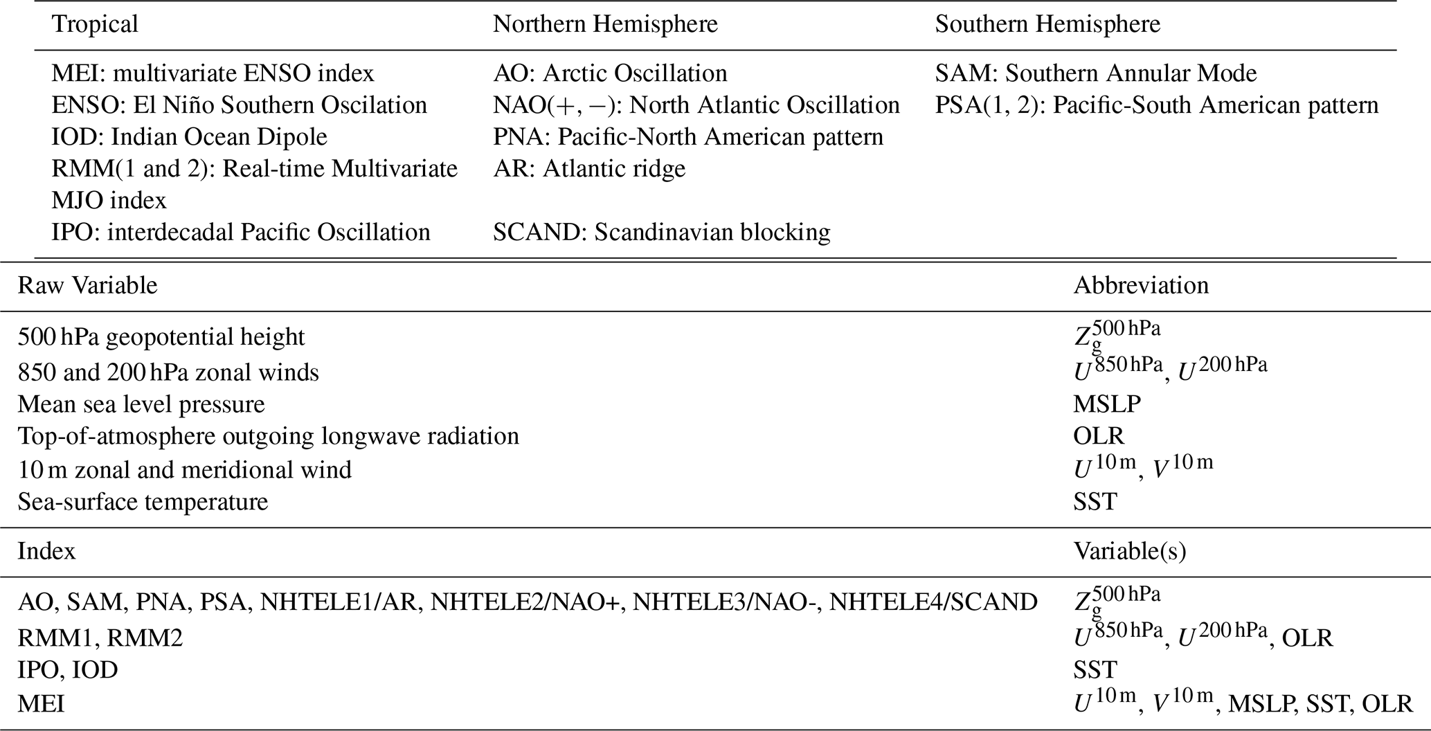
To fully examine tropical interactions we need to understand the MJO, which is considered an eastward moving “pulse” of cloud and rain occurring every 1 to 2 months. The Real-time Multivariate MJO indices RMM1 and RMM2 of Wheeler and Hendon (2004) correspond to a principal component pair formed by projection of daily data onto multivariate empirical orthogonal functions (EOFs) comprised of tropospheric zonal winds (U^{200 hPa,850 hPa}) and outgoing longwave radiation (OLR), with the annual cycle and components of interannual variability removed, such that the time series vary mostly on intraseasonal timescales. Unlike for ERA5, the RMM indices were not able to be calculated for the ACCESS model as the required daily variables are unavailable and so are not present in the inferred ACCESSCM2 networks. For this reason two further Bayesian network experiments using ERA5 inputs with the RMM indices removed were conducted to enable an appropriate comparison with the ACCESS model experiments. Tropical variability induced via SST in the Pacific is incorporated via inclusion of the multivariate ENSO index (MEI) as defined by Zhang et al. (2019) and in the Indian Ocean via the dipole mode index (IOD) (Saji et al., 1999).

The computation of the Southern Annular Mode (SAM) (Rogers and van Loon, 1982), Arctic Oscillation (AO) (Thompson and Wallace, 1998, 2000), and the Pacific South American (PSA) patterns (Mo and Ghil, 1987) are all calculated via EOFs where the loading pattern was computed from the square root cosine weighted monthly anomalies of 500 hPa geopotential height ($Z_{\mathrm{g}}^{\mathrm{500}\mathrm{hPa}}$) relative to a 1979–2001 base period and normalized. Our investigations using this approach on ERA5 for which there were both daily and monthly inputs indicated the impacts of reduced temporal resolution were minor. The Pacific North American (PNA) pattern (Barnston and Livezey, 1987) is constructed as the leading mode obtained after performing a VARIMAX rotation of the first ten EOF modes of monthly standardized anomalies of monthly mean $Z_{\mathrm{g}}^{\mathrm{500}\mathrm{hPa}}$ polewards of 20° N during the boreal winter. The PNA index is then the projection of the standardized height anomalies onto the resulting pattern, standardized by the monthly mean and standard deviation within the aforementioned climatology reference period. Indices of the Pacific South American modes (PSA) (Mo and Ghil, 1987), are defined as the second and third EOF modes calculated from year-round $Z_{\mathrm{g}}^{\mathrm{500}\mathrm{hPa}}$ anomalies polewards of 20° S, projected onto each mode and normalizing by the standard deviation of the corresponding principal component (PC) over the reference period.

Following Straus et al. (2017), the set of four Euro-Atlantic Northern Hemisphere tropospheric teleconnections (NHTELE) are calculated via k-means clustering analysis of the leading 24 PCs of boreal winter $Z_{\mathrm{g}}^{\mathrm{500}\mathrm{hPa}}$ anomalies in the sector 20–80° N, 90° W–30° E computed using monthly anomalies of $Z_{\mathrm{g}}^{\mathrm{500}\mathrm{hPa}}$ rather than the traditional daily values, again with apparent minor impacts on the patterns of the cluster centroids and in comparison to reference indices. Specifically, we consider the North Atlantic Oscillation (NAO) (van Loon and Rogers, 1978), Scandinavian blocking (SCAND), and the Atlantic Ridge (AR) as defined in Table 1.

2.3 Interdecadal Pacific Oscillation

Although a principal component based approach to computing the IPO produces a robust signal of the SST variability associated with the dominant Pacific basin wide variability, and thereby potentially mitigates systematic biases present in some models, the fixed latitude/longitude rectangular boxes of the IPOTPI has been found by us to adequately capture the signal in both our reanalysis and models under investigation, with numerous computational advantages as described by Henley et al. (2015). It is defined by:

$$\begin{array}{}\text{(1)}& \mathrm{IPOTPI}={\mathrm{SSTA}}_{\mathrm{2}}-{\displaystyle \frac{({\mathrm{SSTA}}_{\mathrm{1}}+{\mathrm{SSTA}}_{\mathrm{3}})}{\mathrm{2}}},\end{array}$$

where SSTA is the monthly SST anomaly (relative to same base or entire period) and 1, 2 and 3 denote different regions which are latitude/longitude horizontal boxes defined by the edges 25° N → 45° N/140° E → 145° W, 10° S → 10° N/170° E → 90° W and 50° S → 15° S/150° E → 160° W, respectively.

The application of a moving window applied to the IPO tripole index is a standard approach to isolate multi-decadal variability and for identifying the time periods corresponding to respective phases of the IPO. Here we have chosen a 30-year window as we are primarily interested in the timing of the phase transition if present in the data. The most common choices of window range from 13- to 30-years. Henley et al. (2015) point out that results are qualitatively consistent across three SST reanalysis datasets (HadISST1, HadSST.3.1.0.0, ERSSTv3b) for moving windows of length varying between 10–40 years. We apply the same approach to CMIP model data to augment the number of possible alternate cases of phase transitions beyond the observed historical single case of transition between positive and negative multi-decadal regimes.

To examine causal relationships in physically well established indices of the tropical-extratropical region shown in Table 1 and as used in our previous studies (Harries and O'Kane, 2021; O'Kane et al., 2024), augmented here with the addition of IPOTPI following Eq. (1), we extracted relevant datasets from the ERA5 reanalysis and ACCESSCM2 model simulations. Hereafter we refer to the IPOTPI as simply the IPO. Periods for positive and negative phases of the observed IPO are shown in Fig. 1a and provided in Table 2. The monthly ERA5 IPO is found to be very similar to that derived from the extended reconstruction SST (ERSST) analysis version 5 (Huang et al., 2017) (not shown), as expected. Lowpass filtered and 30 year average moving window results for ERA5 and ERSST identify almost identical positive IPO phases, but are somewhat different during the negative phase due to less consistency in the early observed record in the first two-thirds of the twentieth century. Low pass filtered results obtained by retaining lowest order harmonics (7 modes) shown in Fig. 1 clearly indicate the IPO phases and are generally in agreement with the straight-forward moving window approach which we have implemented.

Table 2 Datasets and the determined IPO phase periods considered.

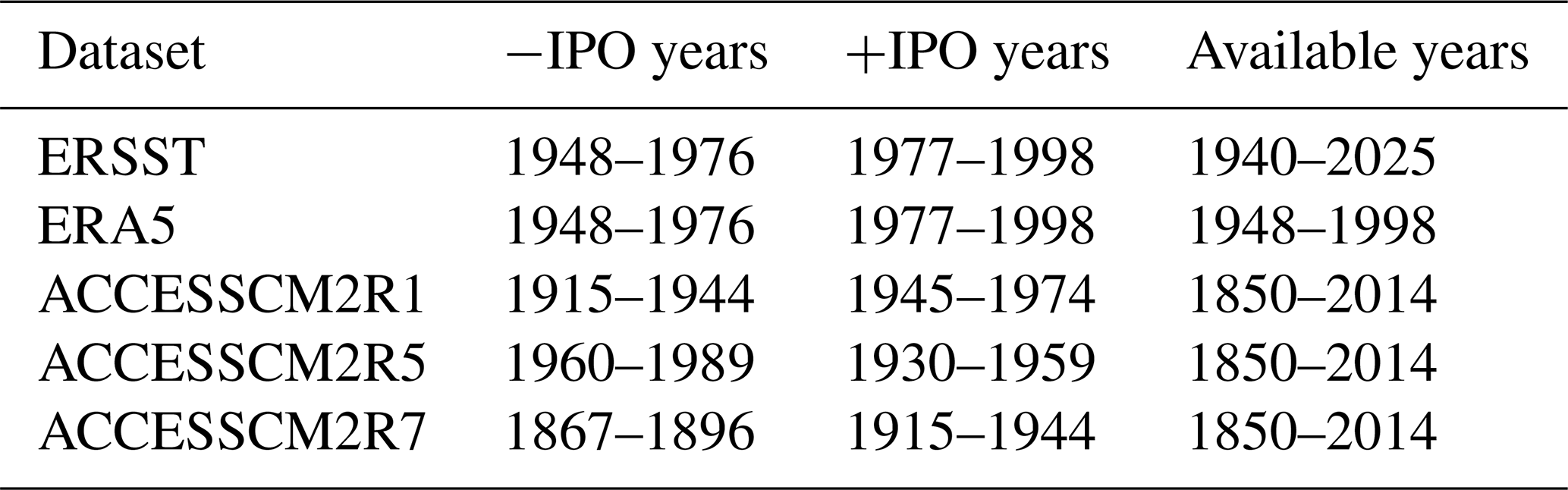
Figure 1 Monthly IPO tripole index values calculated over the period 1940–2024 via Eq. (1) (magenta); and with low pass filter applied by retaining only the leading 7 natural harmonic modes (orange lp nh = 7). Significant negative phases of the IPO occur over the indicated periods 1948–1976 and 1999–present. A prolonged positive phase occurred over 1977–1998.

The observed IPO phases over the second half of the twentieth century are provided in Table 2 and for this we have taken the phase switch year to be between 1976 and 1977. To isolate IPO regime shifts as simulated by the ACCESSCM2 model, we have examined the time-series over the full historical experiment, 1850 to 2014. To identify significant (when compared to what is observed) IPO phases we compute a 30 year moving window on the IPO and manually identify 30 year periods for each where they exist. These are provided in Table 2 for ACCESS and ERA5, and diagramatically in Fig. 1 for the ERA5. The chosen experiments with well defined IPO phases are numbered 1, 5 and 7. The DBN experiments are run separately for each IPO phase as well as over all years spanning the sequential phases, with the exception as follows. For the reanalysis and the ACCESSCM2{1,5} realizations the IPO phases are temporally contiguous, however, with the ACCESSCM2R7 realization the IPO phases are separated by a neutral phase lasting a number of decades. This set of three will allow us to comment on regime shifts versus independent regime events. To better observe the slowly varying component of the IPO in the monthly data often a low pass filter or similar is applied, however, in this case we have left the monthly data unfiltered to be compatible with the other indices, which exhibit significant spectral energy at a range of higher frequencies. The IPO and ENSO indices, for example Niño3.4, co-vary strongly, however, there are exceptions especially during negative IPO events when the extratropical SST anomalies dictate the overall magnitude and sign of the IPO index. During positive IPO events SSTs in the tropics dominate the index, where negative and positive extremes of the IPO index are generally well represented by the Niño3.4 index.

3 Methods

Causal relationships between the selected teleconnections are inferred under the assumption that the system may be adequately described by linear VAR models, represented graphically as DBNs (while the inclusion of a moving average component may yield a better fit for some modes, the use of VAR models somewhat simplifies model implementation). Here we briefly summarize the method used to fit the models, shown schematically in Fig. 2. Further details may be found in O'Kane et al. (2024).

Figure 2 Schematic outline of structure learning strategy.

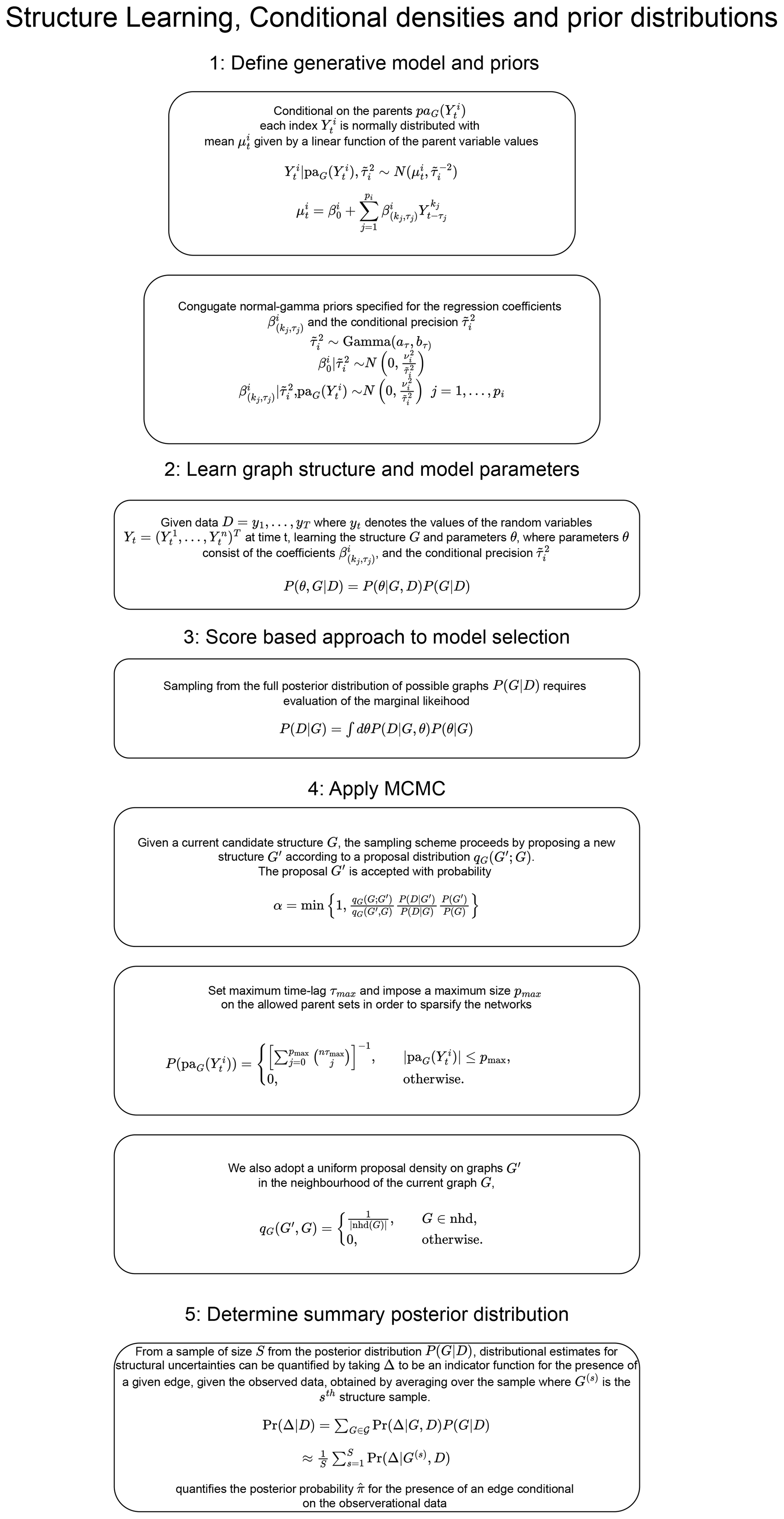
The observed value of each index i in month t, $Y_t^i$, is assumed to be normally distributed with mean ${\mathit{\mu }}_t^i$ and variance ${\stackrel{\mathrm{̃}}{\mathit{\tau }}}_i^{-\mathrm{2}}$ (panel 1 of Fig. 2), with

$$\begin{array}{}\text{(2)}& {\mathit{\mu }}_t^i={\mathit{\beta }}_{\mathrm{0}}^i+\sum _{j=\mathrm{1}}^{p_i}{\mathit{\beta }}_{(k_j,{\mathit{\tau }}_j)}^i{Y}_{t-{\mathit{\tau }}_j}^{k_j}.\end{array}$$

The collection of indices ${\mathrm{pa}}_G\left(Y_t^i\right)=\mathit{\left\{}{Y}_{t-{\mathit{\tau }}_j}^{k_j}\mathit{\right\}}$ upon which $Y_t^i$ depends is referred to as the parent set of $Y_t^i$. Graphically, the model may be represented as a network in which the nodes are the random variables corresponding to the indices and their lagged values, up to some maximum lag τ_max. Directed edges are drawn from the node for each member of the parent set to the node representing the index at time t (the child node). Contemporaneous edges are assumed to be absent, ensuring acyclicity of the graph at the cost of excluding possible interaction taking place on time-scales shorter than the monthly sampling frequency. The resulting graph is assumed to be constant over time, and thus corresponds to a time-homogeneous DBN. To investigate possible changes in the structural relationships associated with changes in the background state, separate models were fitted to periods of positive and negative IPO phase, in addition to the full timeseries. In this respect, we assume that the prescribed IPO phases represents period in which the relationships between the different modes are stationary, and can be inferred by stratifying on IPO phase. While doing so invariably results in some loss of power due to reduced sample size, and may introduce artefacts arising from discretization of what is likely a continuous underlying process, the use of separate models is a simple approach to allow an initial investigation into variability in teleconnections with respect to the background state without dramatically increasing model complexity. The implementation of more realistic non-stationary models may be facilitated by the use of alternative model specifications (Zhou et al., 2024), and is left for future study.

Both the parent sets (i.e., the graph structure) and associated VAR parameters are taken to be unknown, and are inferred from the historical data or model runs. Independent, conjugate normal-gamma priors are assumed for the VAR parameters ${\mathit{\beta }}_{\mathrm{0}}^i$, ${\mathit{\beta }}_{(k_j,{\mathit{\tau }}_j)}^i$, and ${\stackrel{\mathrm{̃}}{\mathit{\tau }}}_i^{-\mathrm{2}}$, with hyperparameters a_τ=1.5, b_τ=20, and ${\mathit{\nu }}_i^{\mathrm{2}}=\mathrm{3}$ (panel 2). Estimation of the graph structure and parameters proceeds in two stages, by writing the joint posterior distribution as a product of conditional distributions (panel 3). The prior specification yields an analytically tractable marginal likelihood (panel 4), thus allowing the MC³ scheme of Madigan et al. (1995) to be used to sample from the posterior distribution over possible graphs P(G|D) (panel 5). Structurally modular, uniform priors over possible parent sets with lags of at most τ_max=6 months and size at most p_max=10 are used (panel 6). The choice of lag for networks based on monthly indices, i.e., ${\mathit{\tau }}_{max}=\mathrm{6}$ months, corresponds to the approximate e-folding time of the MEI and we argue this is an appropriate timescale for tropical variability. This choice also allows direct examination of the influence of IPO phase on the causal relationships between the internal modes relative to their annual and seasonal climatological DAGs recently reported by O'Kane et al. (2024) in their examination of CMIP5 models where the IPO was absent from the parent set.

A uniform proposal distribution over the neighborhood of the current graph is used (panel 7), where the neighborhood of a given graph consists of those graphs that can be obtained from it via addition or deletion of a single edge or exchange of two edges (Grzegorczyk and Husmeier, 2011), subject to the constraints on the maximum lag and parent set size. Posterior samples for each index were obtained by running 8 chains of length 1×10⁷ samples, discarding the first 250 000 samples as a burn-in period, to reduce possible biases associated with samples drawn well before the chain has converged to the target distribution. Chain convergence was assessed by considering the homogeneity of the distribution of parent sets across chains using χ² and Kolmogorov-Smirnov tests (Brooks et al., 2003) for each index, in addition to trace plots for individual edge indicators. Results presented here are based on the full set of posterior samples.

From the sample of graph structures, estimates for the posterior distribution of quantities of interest Δ may be obtained by averaging over the sample (Draper, 1995) (panel 9 Fig. 2). In particular, structural uncertainties may be quantified via an indicator function Δ for the presence of a given edge, with Pr(Δ|D) quantifying the posterior probability $\widehat{\mathit{\pi }}$ for the presence of that edge, conditional on the observed data D. In the following we summarize edges for which $\widehat{\mathit{\pi }}>\mathrm{0.5}$ (both overall and within IPO phases) as summary graphs. It should be noted, however, that these figures summarize the posterior distribution over the candidate VAR models, and do not correspond to any single model, such as the maximum a posteriori (MAP) model.

4 Results and discussion

Before exploring the impact of the IPO phase on inferred dependence relationships, we first assessed the tropical-extratropical causal networks in ERA5 as compared to those in similar state of the art reanalyses as reported previously (Harries and O'Kane, 2021; O'Kane et al., 2024). When the full ERA5 time period is used and the IPO excluded, similar networks were found to those reported for JRA55 and NCEP-NCAR Reanalysis 1 (NNR1) as revealed in Fig. 3a, as compared to Fig. 2 of O'Kane et al. (2024), thereby confirming that the ERA5 DAGs are largely consistent with comparable reanalysis products. Relationships associated with the MJO and ENSO are generally similar, while there are minor differences (mostly at longer lags) with respect to relationships involving lagged extratropical modes. Such differences can arise in part due to various climate model configurations, data assimilation schemes and observing system inputs. Inclusion of the IPO index modifies the posterior edge probabilities identified with tropical interactions (Fig. 3b), most notably enhancing the long autocorrelation time-scales associated with ENSO and MJO indices relative to those of Fig. 3a. There is substantial posterior weight ($\widehat{\mathit{\pi }}>\mathrm{0.7}$) assigned to dependence of the IPO on IPO_t−6 however, the greatest weight is found at one month lag with linkage to ENSO and coupling at t−1 and t−2 to both MJO indices as well as the IOD (Fig. 3a). In particular, Fig. 3b shows the strong tropical coupling of the IPO via central to eastern Pacific SST variations evident in nodes ${\mathrm{IPO}}_{t-\mathrm{1}}\to {\mathrm{MEI}}_{t=\mathrm{0}}$ and to the Maritime Continent via ${\mathrm{IPO}}_{t-\mathrm{2}}\to \mathrm{RMM}{\mathrm{2}}_{t=\mathrm{0}}$. The overall set of relationships with all indices is quite similar whether the IPO is included or not, an indication of the level of strong interdependence of the IPO to the tropical drivers, especially considering when extratropical activity associated with the IPO is high.

Figure 3 Posterior probabilities for edges from ERA5 data over the period 1948–1999: (a) considering all teleconnections excluding the IPO (ALL-IPO); (b) considering all teleconnections including the IPO (All) and (c) considering all teleconnections excluding the MJO (All-MJO). π<0.8 probabilities are dashed for clarity.

The graphs in Fig. 3 indicate Indian and Pacific oceans linkages occur via the MJO (RMM2). Specifically in Fig. 3a, we see the IOD_t−5 connecting to RMM2_t child and the RMM1_t−6 and RMM2_t−2 to the IOD_t child. The MEI has multiple linkages to RMM1_t with RMM1_t−4 with $\widehat{\mathit{\pi }}\ge \mathrm{0.9}$. The MEI also links to the IOD_t−1 ($\mathrm{0.5}<\widehat{\mathit{\pi }}<\mathrm{0.6}$) and RMM2_t−2 ($\mathrm{0.8}<\widehat{\mathit{\pi }}<\mathrm{0.9}$). These relationships are indicative of the Walker circulation and convection over the Maritime Continent on intraseasonal to interannual timescales as the major mechanism teleconnecting tropical Sea Surface Temperatures in the Pacific and Indian oceans. Addition of the IPO (Fig. 3b) enhances the MJO autocorrelation while also adding an edge from IPO_t−1 to the MEI_t child node ($\widehat{\mathit{\pi }}\ge \mathrm{0.9}$) but otherwise the graph is unchanged. The large edge weight between IPO_t−1 and MEI_t is not surprising given the definition of the IPO index Eq. (1).

Removing the MJO child nodes (Fig. 3c) eliminates a crucial branch of the Walker circulation but does not lead to posterior edges not present in the more complete graphs. The directionality of the high probability NAO${}_{t-\mathrm{1}}^{-}$ to RMM2_t reflects the lagged influence of extra-tropical NH variability on the tropics (Kitsios et al., 2019; Stan et al., 2017). Given there are no NH child nodes present, the influence of the tropics on the NAO, i.e., a directed edge from the tropical modes to the NAO child, is not captured. In general we see that, apart from the high latitude AO, the mid-latitude NH extra-tropical modes (NAO⁻, PNA, SCAND) are still present however in the absence of the MJO, their tropical teleconnection transfers to the MEI. The SH PSA and SAM modes are largely unaffected as they teleconnect to the tropics through ENSO directly. Posterior edges between the hemispheres (sans IPO) were comprehensively examined in the study of O'Kane et al. (2024).

The MJO is known to couple to the extratropics via Rossby wave activity, and in particular to the NAO (Kitsios et al., 2019; Stan et al., 2017). From the result shown in Fig. 3c, we observe no IPO autocorrelation beyond the t−1 parent node, rather there is a >0.9 edge weight from the MEI${}_{t-\mathrm{1},\mathit{\&}t-\mathrm{6}}$ months. This is in contrast to Fig. 3a and b, where the MJO teleconnection was observed to mediate the tropical-extratropical interactions. In the absence of the MJO, the MEI${}_{t-\mathrm{1},\mathit{\&}t-\mathrm{6}}$ nodes (and to a lesser degree the IOD node at lag one) links with high probability to the IPO. Comparison of Fig. 3b and c and the relationship between the IPO and the MEI (and IOD), when MJO variability is or is not included, reveals the important role of the MJO in linking the tropics with the extratropics, not only on the intra-seasonal time scale that dominates the regions of the Maritime Continent and tropical Indian Ocean, but as being key to inter-annual ENSO and longer timescale IPO phases.

Comparison of ERA5 networks conditioned on specified phases of the IPO, including or excluding the MJO, are shown in Figs. 4 and 5 for the negative (−IPO: Figs. 4a and 5a) and positive (+IPO: Figs. 4c and 5b) phases, respectively. Where the MJO is not included, it is striking the reduction and/or reallocation that occurs between tropical child indices and their parent nodes, and even more dramatic relative to that which occurred in examining all years (Fig. 3). In the −IPO case when MJO indices are not included (Fig. 5a), almost no parent-child relationships remained apart from autocorrelation in the principal tropical modes i.e., IOD, MEI and IPO; the only NH extratropical parent node occurs for the PNA_t−4. The DBNs for the +IPO phase depict a similar collapse of the IPO autocorrelation with no dependence on any extratropical modes. When the MJO is included in the −IPO network (Fig. 4a), there are generally more interactions at longer time lags occurring for the PNA_t−6, SAM_t−5 and IPO${}_{t-\mathrm{6},t-\mathrm{5}}$. Also, during the +IPO phase (Fig. 4c) a short term t−1 lagged relationship is noted between the NAO⁻ and MJO with a probability between 0.7 and 0.8. The IOD in the +IPO phase is seen to have more parents and stronger evidence for the individual linkages, in particular between the MJO and the IOD and ENSO. This may be expected during the positive IPO phase when higher than average tropical SSTs in regions of the Indian/Pacific oceans are known to induce enhanced tropical-extratropical teleconnections and more frequent and larger amplitude El Niño events. Heidemann et al. (2023) found eastern Pacific El Nino's were observed (lasted) 23 % (10 months) of the time during +IPO periods compared to only 14 % (7 months) during −IPO periods. Furthermore, when IPO and ENSO are in phase, teleconnections around the Pacific basin are strongly enhanced (Yeh et al., 2018).

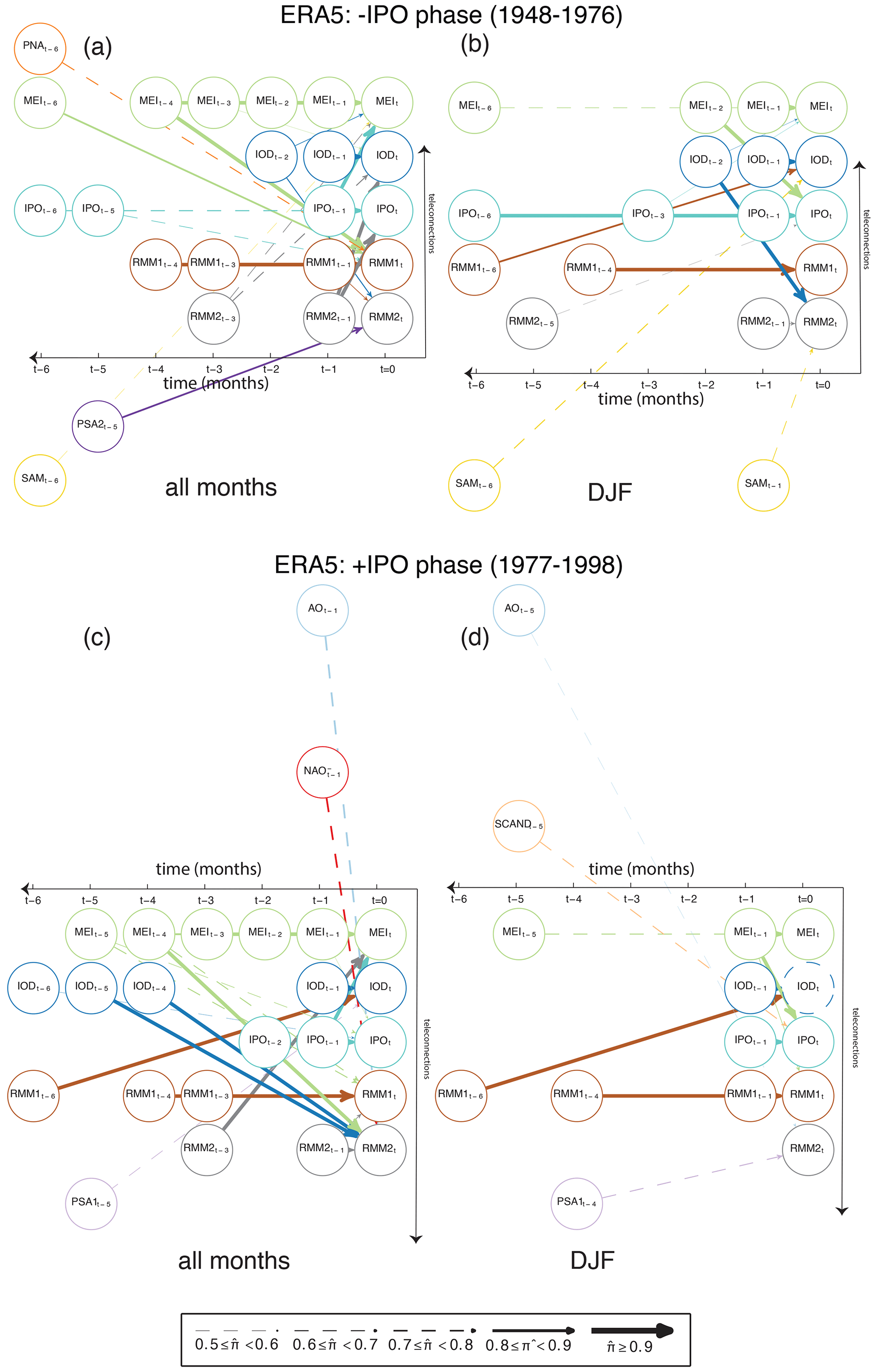
Figure 4 (a) Posterior probabilities for edges from ERA5 data over the (a) negative IPO phase 1948–1976 and (c) the positive IPO phase 1977–1998 considering all months in the designated periods; (b, d) considering only those months during the boreal winter (DJF). π<0.8 probabilities are dashed for clarity.

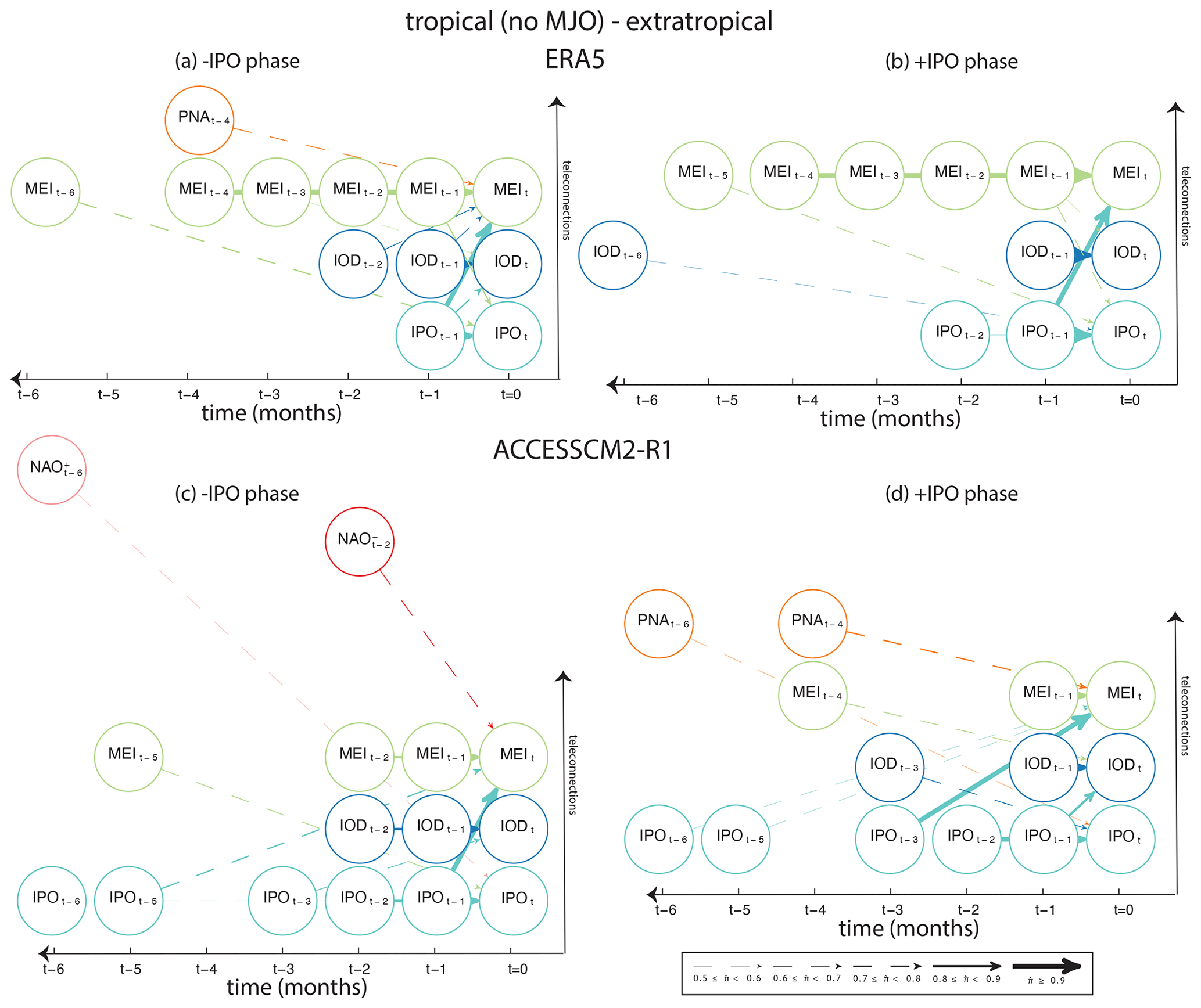
Figure 5 Posterior probabilities for edges from reanalysis and ACCESSCM2 GCM data over historical simulations corresponding to negative (a) ERA5 (c) R1, and positive (b) ERA5, (d) R1; IPO phases described in Table 2. π<0.8 probabilities are dashed for clarity.

Differences between the IPO phase dependent ERA5 networks inferred during the boreal winter DJF) (Fig. 4b and d) to those estimated over all months (Fig. 4a and c) most notably occur during the +IPO phase (Fig. 4c and d), and in particular a weakened lagged influence of the IOD${}_{t-\mathrm{4},\mathrm{\dots },t-\mathrm{6}}$ on the MJO (RMM2_t). Additionally we see weaker autocorrelation in the tropical modes with evidence of influence from synoptic scale blocking activity (SCAND_t−5) and zonal tropospheric flow (AO_t−5) in the NH at longer lag, presumably as a consequence of the seasonally dependent background state. In contrast, there are less substantial differences between the −IPO phase dependent ERA5 networks conditioned over all months (Fig. 4a) and those during the boreal winter (Fig. 4b) where the flow is more strongly influenced by the SAM_t−1 at the expense of the PSA_t−5.

When excluding the MJO child nodes, the lack of strong autocorrelation at lags beyond IPO_t−1 (Fig. 3c) can be understood as follows: the IPO index is defined such that, in the absence of extra-tropical SST influences, it will be dominated by the tropical Pacific SSTs and hence ENSO. One would therefore expect a strong autocorrelation in the MEI at most times with or without the MJO, with the IPO autocorrelation dependent on the strength of the extra-tropical SST anomalies, as our results show. Taking IPO phase and seasonality into account (Fig. 4) we see that long autocorrelation in the IPO occurs for the negative phase but not the positive phase and that this is consistent for conditioning only on the boreal winter. The dominance of tropical Pacific SST variability during the +IPO phase is not unexpected as this period was one where ENSO has been observed to be most active. Removal of the MJO (Fig. 5a and b) further collapses the graph structure to be dominated by the IPO, MEI, and IOD.

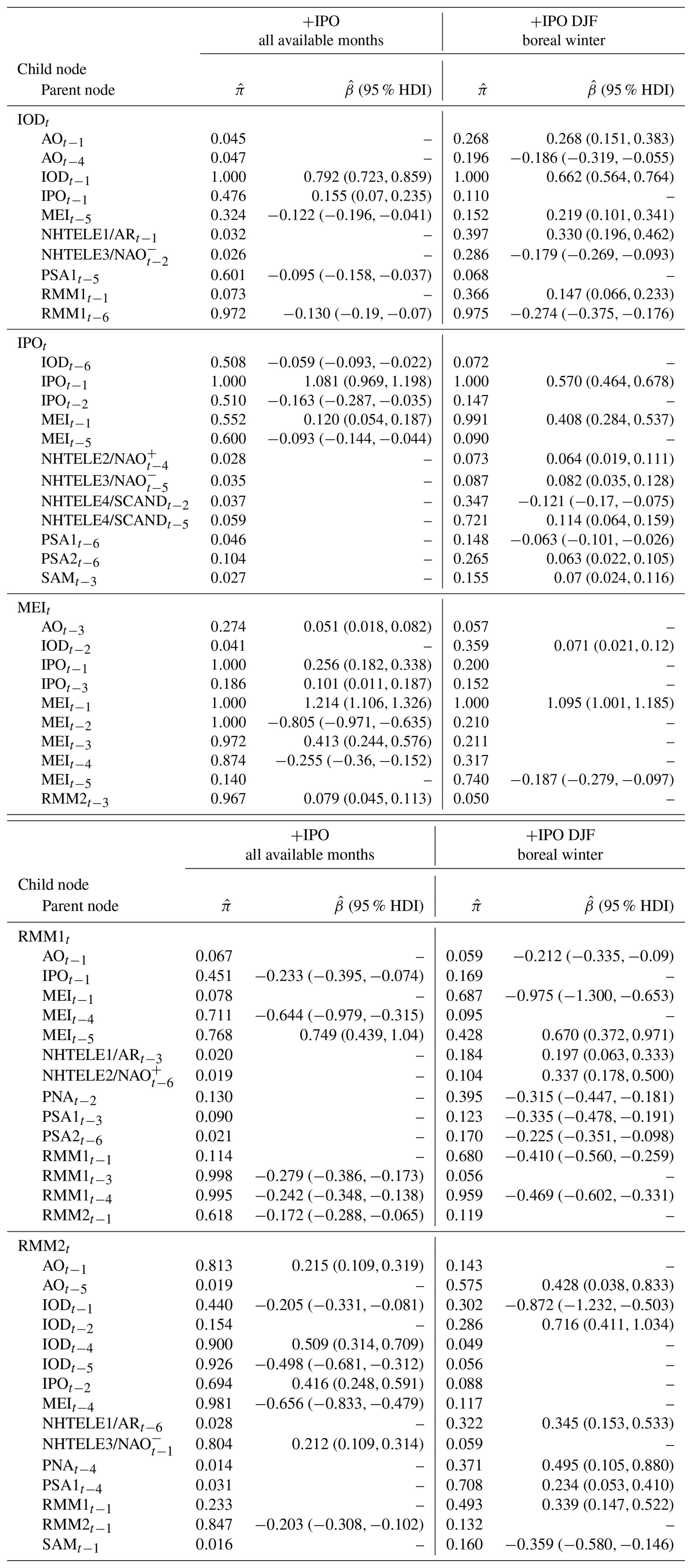
The graphs displayed in Fig. 4 summarize the relationships that, individually, have a relatively high posterior probability when considering all allowed models. Inspection of individual models allows the co-occurrence of particular edges to be examined. The structures of the MAP model for each IPO phase and season, together with the corresponding regression coefficients, are shown in Tables  and . In addition to edges with $\widehat{\mathit{\pi }}>\mathrm{0.5}$, the MAP models also include relationships that improve the fit but have weaker evidence to support their inclusion. For example, in addition to the associations involving Scandinavian blocking and the AO and the tropical modes, additional interactions for which $\widehat{\mathit{\pi }}<\mathrm{0.5}$ between other extratropical modes and tropical modes are found in the MAP model for the boreal winter during the positive IPO phase.

Table 3 ERA5 MAP parent sets for the IPO and tropical climate indices across all available months, and for the boreal winter (DJF) conditioned on the −IPO phase for fits with a_τ=1.5, b_τ=20, and ν²=3, showing the estimated posterior mean $\widehat{\mathit{\beta }}$ conditional on the MAP structure, and the 95 % posterior highest density interval (HDI). Dashes indicate a node that is not in the MAP parent set for a given phase and or season.

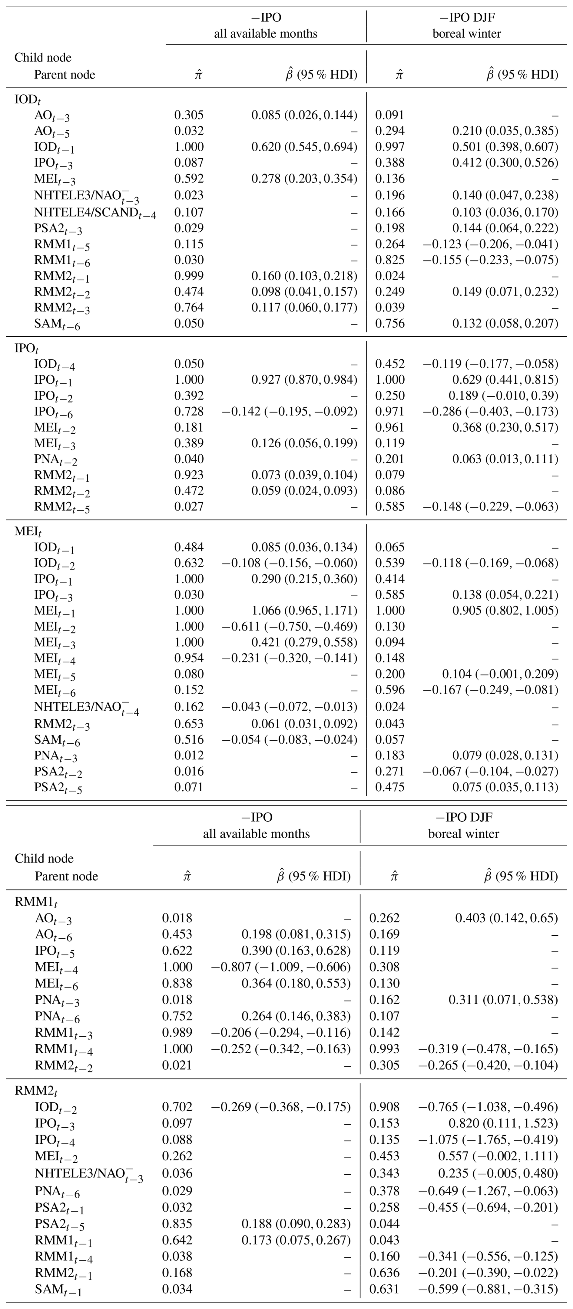
Table 4 ERA5 MAP parent sets for the IPO and tropical climate indices across all available months, and for the boreal winter (DJF) conditioned on the +IPO phase for fits with a_τ=1.5, b_τ=20, and ν²=3, showing the estimated posterior mean $\widehat{\mathit{\beta }}$ conditional on the MAP structure, and the 95 % posterior highest density interval (HDI). Note. Dashes indicate a node that is not in the MAP parent set for a given phase and or season.

Lastly, we turn our attention to the results for the identified IPO regimes in the ACCESSCM2 climate model. As noted in Sect. 2, daily data are not available from which to derive MJO indices and so are not included in summary statistics for comparison to the reanalysis. Instead, our aim is to examine the potential diversity of networks across IPO phases for a number of cases. This is not possible using reanalyses due to the restricted time period over which observations are available. While our focus here is to examine changes to the summary statistics during IPO phase transitions within a modeling context, we also compare to those we have already identified in the ERA5 reanalysis to ascertain potential model biases including autocorrelation and the range of displayed internal variability.

Like many models, the ACCESSCM2 model exhibits bias in the SST spatial pattern representing the leading principal component from singular value decomposition analysis; specifically an ENSO-like pattern that extends too far west and somewhat equatorially confined relative to ERA5. There are in addition regional SST biases, for example, the somewhat weak SST anomalies over the Tropical Indian Ocean also observed in other CMIP6 models (Chinta et al., 2023). That said, the availability of an ensemble of ACCESSCM2 historical simulations enables qualitative investigation of the potential diversity of teleconnections over recent decades. In particular, we are interested in the ENSO autocorrelation relative to the IPO autocorrelation during +IPO and −IPO phases, and in comparison to the case where the IPO is not included in the DBN model. Despite being unable to include an MJO index, we take the opportunity to compare CGCM DBNs to ERA5 DBNs with and without the MJO so as to infer the role of the MJO in communicating extratropical disturbances to organized tropical intraseasonal variability, e.g., Kitsios et al. (2019) and discussions therein.

Described in Table 2 are the three ACCESSCM2 cases of IPO transition considered, namely negative directly to positive (ACCESSCM2R1: Fig. 5c and d), positive directly to negative (ACCESSCM2R5: Fig. 6e and f), and a 19 year neutral period prior to transitioning from negative to positive (ACCESSCM2R7: Fig. 6g and h). These differences directly impact the graphs as the climatic features that “trigger” the transitions would be expected to be quite different. It is apparent that there is considerable diversity in the DBNs across each of the transition cases considered. The extent and weight of the simulated tropical-extratropical posterior edge probabilities is greater than those seen in ERA5 (MJO excluded). In particular, the extratropical indices such as the PNA, NAO${}^{+,-}$ and AR parent nodes at long lags (3–6 months) with high posterior edge probability to tropical indices (MEI, IPO) are particularly evident in the −IPO phase relative to the +IPO phase. These differences are especially apparent in the ACCESSCM2R5 and ACCESSCM2R7 IPO transitions displaying somewhat similar posterior edges e.g., to the PNA, NAO${}^{+,-}$. In the ACCESSCM2R5 model −IPO phase we observe a high posterior edge probability between the IPO_t−1 and the IOD not seen in the other five model based DAGs. During the −IPO, associated with relatively cool SSTs in the equatorial Pacific, the SSTs of the eastern Indian ocean are in phase with the north-west Pacific and further associated with relatively high temporal standard-deviations and a plausible inter-basin teleconnection across the Sea of Islands and the Maritime Continent. However, if the MJO were to be included in the ACCESSCM2 model graphs, then we would expect there to be evidence of the MJO interacting with the other modes, as was found with the ERA5 case albeit in both IPO phases (RMM2_t−1 and RMM1_t−6 $-/+$IPO, respectively). The observed ERA5 IOD${}_{t-\mathrm{1},t-\mathrm{2}}$ parent nodes link to the MEI_t=0 child, present in the −IPO phase but not in the +IPO, does not appear in any of the modeled networks.

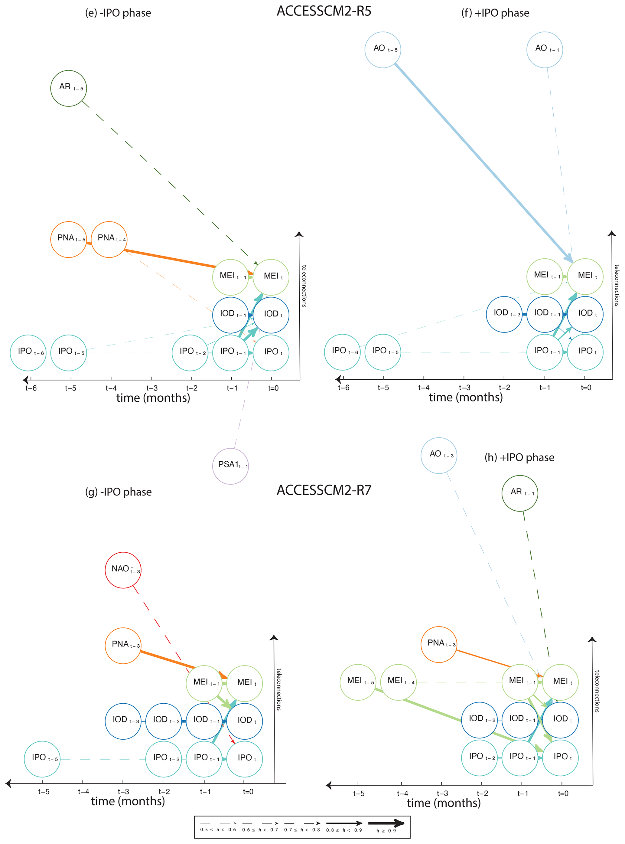
Figure 6 Posterior probabilities for edges from ACCESSCM2 GCM data over historical simulations corresponding to negative (e) R5, (g) R7 and positive (f) R5, (h) R7; IPO phases described in Table 2. π<0.8 probabilities are dashed for clarity.

It remains to comment on the relationship between inferred links i.e., edges in the DAGs, and the physical interpretation and implications of lagged statistical causality in relation to established mechanistic understanding of atmospheric teleconnections. In particular, that the graphs are directed and acyclic affords easy interpretability w.r.t. the direction of influence i.e., the arrow of time. Take for example the graphs for the ERA5 MJO child and NAO parent nodes depicted in Fig. 3. There we see strong northern extratropical influence of the NAO⁻ phase on RMM2 at 1-month lag. Physically this indicates the occurrence of the NAO⁻ phase leading the MJO is dynamically important. Lin et al. (2021) showed that for the majority of seasonal prediction models, MJO prediction skill is highly dependent on the amplitude and phase of the NAO in the initial condition and that where predictions are initialized from a strong NAO⁻, the skill in predicting the MJO is increased. The AO is also seen to influence the MJO at 1-month lag potentially revealing the combined effects of the background state on the MJO. A popular physical mechanism for the observed NAO-MJO relationship is posited in terms of extratropical Rossby wave propagation (Stan et al., 2017) however, studies of the NAO-MJO relationship have mainly examined the influence of the tropics on the extratropics, therefore requiring inclusion of NAO child nodes in the DAGs as was done in the studies of Harries and O'Kane (2021) and O'Kane et al. (2024). Notably, Lin et al. (2019) showed that the NAO does indeed modulate the subsequent behavior of the MJO at approximately 20 d lag following a strong NAO occurring, and that this tends to predominantly occur during MJO phases 7 and 3, respectively. However, the relationship of NAO phase to any of the particular eight phases of the MJO requires daily rather than the monthly averaged data employed here, which is for future study.

Taking a Bayesian approach to causality potentially identifies relationships that are sometimes hard to discern using standard correlation methods. For example, it is well known that the Southern Hemisphere climate is strongly influenced by low lattitude variations of ENSO and high latitude variations of SAM. Dätwyler et al. (2020) contend that limitations in the length of the instrumental record limits knowledge of the SAM-ENSO relationship through time. Our analysis (Fig. 3) shows that where the IPO is present, SAM is seen to have a statistically significant influence on ENSO at 6-months lag. Dätwyler et al. (2020) further point to evidence in the longer paleo record that large amplitude anomalous states of the IPO are seen to occur during periods when SAM and ENSO indices are anticorrelated thereby providing some support that the IPO is important to establishing a SAM-ENSO causal link. It is important to note that the DAGs shown point to the probability that causal relationships exist however, verification and understanding of the mechanisms by which they arise requires detailed investigation of the data from which the graphs are generated.

5 Conclusions

Our objective in this study has been to better characterize regime dependencies via Granger causal graphs corresponding to observed and simulated phases of multi-decadal variations in the IPO. We find not only lagged autoregressive effects but also changes in tropical-extratropical relationships due to dependencies on the phase of the large scale background state, including high confidence levels for those estimates.

Our analysis noted a degree of consistency between ERA5 and earlier published results for NNR1 and JRA55 when conditioned over the same period and tropical regions. Not only does this provide confidence in the results, but it underscores the important role of data assimilation in reanalyses required to constrain the phase relationships of the internal modes of variability. When conditioned on the 1948–1998 time series, inclusion of the IPO index into the considered set of input random variables does not significantly change the posterior edge weights, whereas removal of the MJO impacts both the ENSO and IPO autocorrelation with additional loss of causal relationships between the AO and modification to the PNA teleconnection to the tropics. The latter case reveals the importance of the MJO as a conduit to communicate extratropical variability to the tropics.

Substantive systematic differences between the graphs for positive and negative phases of the ERA5 IPO are found to occur, most notably in the IOD and IPO autocorrelation. IPO autocorrelation for the −IPO phase extends out to t−6 with weaker evidence of interactions between the MJO and IOD. For the +IPO phase, IPO autocorrelation reduces to t−2 but the IOD autocorrelation is very much enhanced with substantial posterior edge weights observed between the MJO and IOD at longer lag. Where the MJO is removed from the input data, the DBN structures collapse to largely IOD-ENSO-IPO nodes further indicating the importance of tropical convection over the Maritime Continent.

Summarizing the analysis of DAGs conditioned on ERA5:

• Inclusion of the IPO index does not substantially modify networks when conditioned over $-/+$IPO phases

• Networks conditioned on the −IPO phase are largely similar to those conditioned on both phases

• Networks conditioned on the +IPO phase are substantially different to the −IPO, showing increased IOD autocorrelations; reduced IPO autocorrelation; enhanced lagged posterior edge weights from MJO parent nodes to the IOD and ENSO

• Exclusion of MJO indices removes important tropical-extratropical linkages while increasing posterior edge weights between ENSO parent nodes and the IPO and IOD child nodes

• Networks conditioned on the boreal winter are sparse with respect to those conditioned on all months of the year

Finally, we attempt to estimate regime dependencies under several transition scenarios. Due to the restricted observational record, we employ the ACCESSCM2 ocean-atmosphere coupled model ensemble simulations with historical radiative forcing. Here we do not expect the model simulations to reproduce the observed phases of the internal modes of variability, however we were surprised by the diversity of IPO phase transitions given the same external forcing applied. A further restriction was the unavailability of full historical period daily data with which to calculate an MJO index, the omission of long continuous set of daily data critical for many studies is a common issue for CMIP submissions. In general, we found DBNs for the three considered cases to be quite diverse with teleconnections to the large scale synoptic tropospheric modes of the Northern Hemisphere i.e., PNA, NAO & AO; and long IPO autocorrelation but systematically much weaker ENSO autocorrelation, that are not reflected in the ERA5 −IPO → +IPO transition. This in part reflects known biases in ACCESSCM2 ENSO power density spectrum (Bi et al., 2020), but also indicates the need to develop systematic causal inference methodologies to better understand regime dependencies manifest in the coupling and phase relationships between the major modes of internal climate variability.