On process-oriented conditional targeted covariance inflation (TCI) for 3D-volume radar data assimilation

This paper addresses a major challenge in assimilating 3D radar reflectivity data with a localized ensemble transform Kalman filter (LETKF). In the case of observations with significant reflectivity and small or zero corresponding simulated reflectivities for all ensemble members, i.e., when the ensemble spread is vanishing, the filter ignores the observations based on its low-variance estimate for the background uncertainty. For such low-variance cases, the LETKF is insensitive to observations and their contribution to the analysis increment is effectively zero. Targeted covariance inflation (TCI) has been suggested to deal with the ensemble spread deficiency (Yokota et al., 2018; Dowell and Wicker, 2009; Vobig et al., 2021). To actually make TCI work in a fully cycled convective-scale data assimilation framework, here we will introduce a process-oriented approach to the TCI in combination with a conditional approach formulating criteria under which targeted covariance inflation is efficient.

The process-oriented conditional TCI addresses the challenge of underrepresented reflectivity in the prior by constructing artificially simulated reflectivities for each ensemble member based on current observations and typical convective processes. Furthermore, certain conditions are used to restrict this spread inflation process to a carefully selected minimal set of eligible observations, reducing the noise introduced into the system.

We will describe the theoretical basis of the new TCI approach. Furthermore, we will present numerical results of a case study in an operational framework, for which the TCI is applied to radar observations at each hourly assimilation step throughout a data assimilation cycle. We are able to demonstrate that the TCI is able to clearly improve the assimilation of radar reflectivities, making the system dynamically generate reflectivity that would otherwise be missing. Related to this, we are able to show that the fractional skill score of radar reflectivity forecasts over lead times of up to 6 h is significantly improved by up to 10 %. All of the results are based on the German radar network and the ICON-D2 model covering central Europe.

1 Introduction

Data assimilation techniques (Lorenc et al., 2000; Rabier et al., 2000; Lorenc, 2003; Liu et al., 2008; Evensen, 2009; Van Leeuwen, 2009; Kleist et al., 2009; Nakamura and Potthast, 2015; Houtekamer and Zhang, 2016; Bannister, 2017; Gustafsson et al., 2018) are employed for the estimation of initial conditions that are used for the initialization of dynamical forecast models. For this purpose, data assimilation techniques combine information from newly measured meteorological observations and previous model forecasts. Considering the special class of ensemble data assimilation techniques (Evensen, 1994; Houtekamer and Mitchell, 1998; Evensen and van Leeuwen, 2000; Houtekamer and Mitchell, 2001; Anderson, 2001; Houtekamer and Mitchell, 2005; Houtekamer et al., 2005; Houtekamer and Zhang, 2016; Potthast et al., 2019; Schenk et al., 2022), an ensemble of atmospheric model states is used to represent uncertainties and correlations between model variables. The usage of such an ensemble of states also allows the calculation of correlations between model variables and atmospheric observations as well as weighting of the information contained in the observations and model variables. Belonging to this group of ensemble data assimilation techniques are the many versions of the particularly popular ensemble Kalman filter (Evensen, 2009), of which the localized ensemble transform Kalman filter (LETKF) (Hunt et al., 2007) is the one most relevant for this present work.

Predicting convective events with numerical weather prediction (NWP) models is challenging due to errors in the initial conditions and the atmosphere's chaotic behavior. Weather radar observations, such as reflectivity and radial winds, can significantly reduce these errors by capturing the 3D evolution of convective systems with high spatiotemporal resolution. The use of radar data to improve convective initiation and forecasting dates back to Lin et al. (1993), who developed a method to initialize convective models by adding humidity in areas with radar echoes. More recently, radar observations were successfully applied in convective-scale data assimilation, significantly enhancing convective storm predictions in NWP models (Gustafsson et al., 2018), with the ensemble Kalman filter – known for its flow-dependent covariances – being widely used in this context. The potential to assimilate radar observations at convective scales was demonstrated in idealized setups (Snyder and Zhang, 2003; Caya et al., 2005; Tong and Xue, 2005; Xue et al., 2006; Gao and Xue, 2008; Sobash and Stensrud, 2013; Lange and Craig, 2014; Thompson et al., 2015; Gao et al., 2016; Lange et al., 2017; Potvin et al., 2017; Bachmann et al., 2019, 2020; Zeng et al., 2021) and in real-data assimilation (Bick et al., 2016; Gastaldo et al., 2018; Zeng et al., 2018; Duda et al., 2019; Zeng et al., 2019; Ruckstuhl and Janjić, 2020; Zeng et al., 2020; Shen et al., 2020).

In this study, we employ the data assimilation framework KENDA (Kilometere-scale ENsemble Data Assimilation) (Schraff et al., 2016), which combines an implementation of the LETKF that closely follows Hunt et al. (2007) and the regional ICON-D2 model, a limited-area mode configuration of the ICON (ICOsahedral Nonhydrostatic) model (Zängl et al., 2015; Prill et al., 2024) that covers central Europe. Considering the assimilation of radar data, KENDA operationally assimilates radar data by employing 3D radar observations obtained from the C-band radar network of the German Weather Service and model equivalents computed by means of the radar forward operator EMVORADO (Efficient Modular VOlume scan RADar Operator) (Zeng et al., 2016). In addition to the assimilation of 3D radar data, KENDA includes the latent heat nudging (LHN) mechanism (Stephan et al., 2008; Schraff et al., 2016), which is based on radar composites of radar precipitation scans.

One of the main challenges of assimilating radar reflectivities with an ensemble data assimilation system like the LETKF is dealing with observations whose corresponding background reflectivity spread vanishes. This vanishing ensemble spread leads to overconfidence in the background system state, and, as a result, the LETKF is unable to adequately employ the information given through such observations and effectively rejects them – even in the presence of large discrepancies between observed and simulated reflectivities. In practical applications it may then happen that the LETKF effectively ignores the information given through the observation of even very large-reflectivity cells and fails to synchronize the true system state, i.e., nature, with the model state.

The purpose of the TCI approach (Yokota et al., 2018; Dowell and Wicker, 2009; Vobig et al., 2021) employed in this work is to overcome the issue just mentioned, i.e., to address the issue of missing ensemble variability and, thus, to make the LETKF more sensitive to observations in cases where observations show that the ensemble does not capture the processes adequately. To this end, artificially simulated reflectivities are constructed and assimilated. The studies of Yokota et al. (2018), Dowell and Wicker (2009), and Vobig et al. (2021) suggest that adding spreads in a targeted way can help make the LETKF take up the observations and draw the fields in the right direction. However, it turns out that applying the scheme in a naive way to the whole domain in a cycled convective-scale framework generates a lot of noise in the system and, even though it helps in selected situations, it worsens the overall scores of both reflectivity forecasts and conventional variables.

To overcome the above problems with the TCI scheme, we will introduce two key techniques into the system. Firstly, the construction is accomplished by means of a specifically designed model that employs selected model variables as independent variables and that has been trained on data found exclusively in the nearest spatiotemporal vicinity of early-stage convective events – defined as regions where the model has just begun to generate significant reflectivity. This algorithm is therefore designed to capture those empirically observed correlations that are most relevant to convective events and the involved physical processes related to their initiation. Using this algorithm for the construction of artificially simulated reflectivities and assimilating them, we expect the system to be pulled towards an overall state that is related to a (pre)convective environment and that is more likely to dynamically produce reflectivity.

Secondly, we employ a particular set of observation selection rules to ensure that the TCI is only applied to the most relevant observations, which usually represent only a very small percentage of the total number of observations. We found that these observation selection rules are essential for minimizing negative effects on the system state. This is particularly relevant in the context of the TCI being potentially applied to all radar data at multiple time steps throughout long-term cycled data assimilation experiments, as this could lead to “accumulation effects”, such as the gradual buildup of errors or biases over time due to periodic changes to the assimilation process introduced by the TCI algorithm.

Regarding an earlier implementation and study of the TCI approach (Vobig et al., 2021), we are already able to demonstrate that, in the context of non-cycled single-observation experiments assimilating only single isolated observations at single time steps, positive effects are introduced into the system in the form of newly emerging simulated reflectivity cells. While this earlier TCI implementation is based on the same general idea, there are several substantial differences between the current version presented here and its predecessor, not only regarding methodological aspects, but also regarding the types of assimilation experiments. Firstly, we completely redesigned the algorithm the TCI approach is relying on for the calculation of artificially simulated reflectivities, using preconvective situations only. Secondly, we established observation selection rules for applying the TCI to carefully selected observations only where a set of criteria is satisfied. Thirdly, we are processing all 3D radar observations available to our system. Lastly, we are studying longer-term NWP data assimilation cycles in an operational setup for which the TCI is applied at each hourly assimilation step – allowing accumulation effects to build up.

Our implementation of the LETKF in the KENDA system is described in Sect. 2.1, the ICON-D2 model setup is summarized in Sect. 2.2, the radar forward operator EMVORADO is explained in Sect. 2.3, and a brief explanation of the latent heat nudging approach is given in Sect. 2.4. We will introduce and describe the process-oriented TCI in Sect. 3.1, describe the conditional approach in Sect. 3.2, and provide more details on the implementation in Sect. 3.3.

The case study upon which the numerical results presented in this work are based is described in Sect. 4.1, together with its particular setup. In Sect. 4.2, we will demonstrate the positive effects of the TCI on the basis of studies of individual cases at single times. In Sect. 4.3, we will discuss the statistical evaluation of longer-term NWP experiments, showing that the fractional skill score (FSS) (Roberts and Lean, 2008) with respect to the reflectivity prediction of free forecast model runs is clearly improved through the TCI by up to 10 % while keeping the negative impact on observation error statistics at a minimum.

2 ICON-KENDA ensemble data assimilation system

2.1 Data assimilation: LETKF

The KENDA system (Schraff et al., 2016) employs the LETKF as suggested by Hunt et al. (2007). This formulation allows us to easily add new observations to the assimilation, while the core implementation can be kept once it is implemented. In the KENDA data assimilation system, the deterministic member represents the best estimate of the atmospheric state, while the ensemble members capture the range of possible states and uncertainties used to generate corrections to improve the deterministic member.

The formulation of Hunt et al. (2007) – see also Nakamura and Potthast (2015, Chap. 5) – solves the Kalman filter equations in ensemble space defined by the ensemble members x^(b,ℓ) for $\mathrm{\ell }=\mathrm{1},\mathrm{\dots },L$ minus the ensemble mean

$$\begin{array}{}\text{(1)}& {\overline{x}}^{\left(b\right)}:={\displaystyle \frac{\mathrm{1}}{L}}\sum _{\mathrm{\ell }=\mathrm{1}}^L{x}^{(b,\mathrm{\ell })}.\end{array}$$

We use the notation

$$\begin{array}{}\text{(2)}& {\mathbf{X}}^b:=(x^{(b,\mathrm{1})}-{\overline{x}}^{\left(b\right)},\mathrm{\dots },x^{(b,L)}-{\overline{x}}^{\left(b\right)})\end{array}$$

for the matrix of ensemble differences from the mean and (for the case of linear H)

$$\begin{array}{}\text{(3)}& {\mathbf{Y}}^b:=H{\mathbf{X}}^b\end{array}$$

for the ensemble differences in observation space, with y^o the observation vector and ${\overline{\mathit{y}}}^b$ the mean of observations simulated from the ensemble. The observation error covariance matrix is denoted by R. Now, we employ Eqs. (20) and (21) of Hunt et al. (2007), i.e.,

$$\begin{array}{}\text{(4)}& {\stackrel{\mathrm{‾}}{\mathit{w}}}^a={\stackrel{\mathrm{̃}}{\mathbf{P}}}^a\left({\mathbf{Y}}^b{)}^T{\mathbf{R}}^{-\mathrm{1}}\right({\mathbf{y}}^o-{\stackrel{\mathrm{‾}}{\mathit{y}}}^b),\end{array}$$

to calculate the mean of the analysis ensemble and ${\stackrel{\mathrm{̃}}{\mathbf{P}}}^a$ given by

$$\begin{array}{}\text{(5)}& {\stackrel{\mathrm{̃}}{\mathbf{P}}}^a=\left[\right(L-\mathrm{1})\mathbf{I}+({\mathbf{Y}}^b{)}^T{\mathbf{R}}^{-\mathrm{1}}{\mathbf{Y}}^b{]}^{-\mathrm{1}},\end{array}$$

where we use the letter L for the number of ensemble members, the notation ${\stackrel{\mathrm{‾}}{\mathit{w}}}^a$ for the linear coefficients of the analysis mean, and I for the identity matrix. ${\stackrel{\mathrm{̃}}{\mathbf{P}}}^a$ denotes the L×L analysis covariance in the space of ensemble coefficients. Equation (2) in the model space leads to Eqs. (22) and (23) of Hunt et al. (2007):

$$\begin{array}{}\text{(6)}& {\displaystyle }{\stackrel{\mathrm{‾}}{\mathit{x}}}^a& {\displaystyle }={\stackrel{\mathrm{‾}}{\mathit{x}}}^b+{\mathbf{X}}^b{\stackrel{\mathrm{‾}}{w}}^a,\text{(7)}& {\displaystyle }{\mathbf{P}}^a& {\displaystyle }={\mathbf{X}}^b{\stackrel{\mathrm{̃}}{\mathbf{P}}}^a({\mathbf{X}}^b{)}^T,\end{array}$$

where ${\stackrel{\mathrm{‾}}{\mathit{x}}}^a$ is the analysis mean and P^a is the analysis covariance matrix. W is calculated by

$$\begin{array}{}\text{(8)}& \mathbf{W}=\left[\right(L-\mathrm{1}){\stackrel{\mathrm{̃}}{\mathbf{P}}}^a{]}^{\mathrm{1}/\mathrm{2}}.\end{array}$$

As in Eq. (24) of Hunt et al. (2007), the analysis ensemble is calculated by

$$\begin{array}{}\text{(9)}& {\mathbf{X}}^a={\mathbf{X}}^b\mathbf{W},\end{array}$$

where the power $\mathrm{1}/\mathrm{2}$ denotes the symmetric square root of the symmetric matrix ${\stackrel{\mathrm{̃}}{\mathbf{P}}}^a$ given by Eq. (5).

It is obvious that, in the case where the ensemble of simulated reflectivities has a small or zero spread, the matrix Y^b (see Eq. 3) has small or zero entries, and in that case both P^a (see Eq. 7) and the transform matrix W (see Eq. 8) are small, such that the ensemble analysis increments given by X^a (see Eq. 9) are small as well. The goal of targeted covariance inflation is to change Y^b in such a way that the reflectivity observations lead to appropriate increments in the humidity and further variables. The basic challenge of different approaches to the TCI is how to construct the inflated matrix Y^b such that the increments avoid spurious noise and generate meaningful convective processes in the model propagations following the analysis steps in a cycled data assimilation framework. We will develop the process-oriented and conditional approaches in Sect. 3.

2.2 NWP model: ICON-D2

The ICON modeling framework (Zängl et al., 2015; Prill et al., 2024) is the numerical weather prediction and climate modeling system collaboratively developed by various institutions and weather services where the Deutscher Wetterdienst (DWD) and the Max Planck Institute for Meteorology (MPI-M) are major contributors. At DWD, the ICON system runs operationally on a global scale, within the European subdomain known as ICON-EU and in the convection-permitting local-area-mode ICON-D2. The model domain of ICON-D2 covers all of Germany, Switzerland, Austria, and parts of the other neighboring countries; see Fig. 1. Therefore, the ICON-D2 model is very similar to that of the former operational COSMO-D2 model¹ (Baldauf et al., 2011), which it replaced in 2021. In this work we mainly employ the ICON-D2 configuration for our model simulations, which have a model resolution of 2.1 km, 65 vertical levels, and lateral boundary conditions provided by ICON-EU simulations.

Horizontally, the ICON model uses an unstructured triangular grid, while in the vertical dimension a distinct set of levels $\mathit{\left\{}{l}_i\right|\mathrm{1}\ge i\ge N\mathit{\}}$ is defined. See Fig. 1 for a rough estimate of the height of each ICON level. Furthermore, the ICON model solves an equation system based on a distinct set of prognostic variables. Generally speaking, a two-component system is assumed involving dry air and water as variables where the latter may appear in all three phases. For a more in-depth discussion of the ICON model, see Prill et al. (2024).

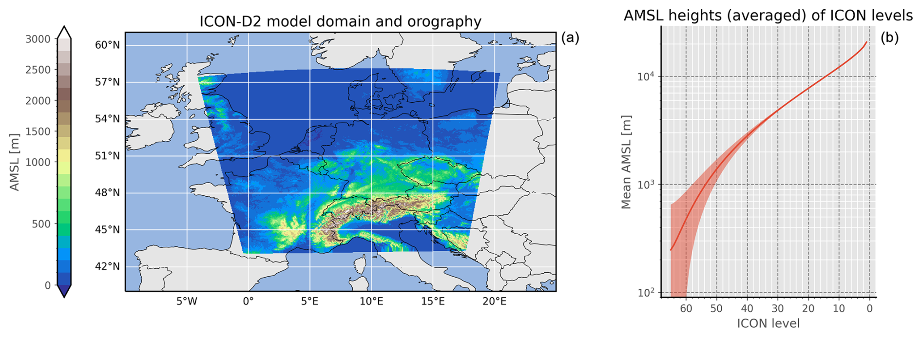
Figure 1 (a) Depiction of the ICON-D2 model domain covering central Europe. The colors indicate the height above mean sea level (a.m.s.l.) of the lowest ICON level that coincides with the ground level. (b) Taking the horizontal mean over the complete model domain, the mean of the a.m.s.l. heights of each ICON level is shown. The shaded areas indicate the related standard deviation.

2.3 Radar forward operator: EMVORADO

In the convective-scale ICON-D2 configuration of the ICON model, 3D radar observations obtained from the German radar network are employed (Bick et al., 2016). The German radar network consists of 17 dual-polarization C-band Doppler radar stations that comprehensively cover Germany (see Fig. 2). The scanning procedure for 3D-volume scans at each radar station involves a complete 360° azimuthal sweep with a 1° resolution at 10 elevation angles ranging from 0.5 to 25°. Radially, the distance reaches up to 180 km for each station, with a resolution of 1 km.

To assimilate 3D radar observations, synthetic 3D radar data are derived from model variables utilizing the EMVORADO forward operator (Zeng et al., 2016), where, considering only its single-polarization implementation in this study, Doppler velocities and reflectivities are computed. Note that simulated radar observations are produced in the observation space; i.e., for each observation, an associated model equivalent is computed. Furthermore, EMVORADO accounts for various intricate physical factors related to the simulation of radar measurements, e.g., beam bending, beam broadening, beam shielding, Doppler velocity with fall speed and reflectivity weighting, attenuated reflectivity, and a detectable signal. The EMVORADO operator also allows superobbing, i.e., the local spatial averaging of observations and corresponding observation equivalents as a standard technique for assimilating spatially high-resolution observations. For more comprehensive information and specifics that are beyond the required scope of this work, please refer to Zeng et al. (2016).

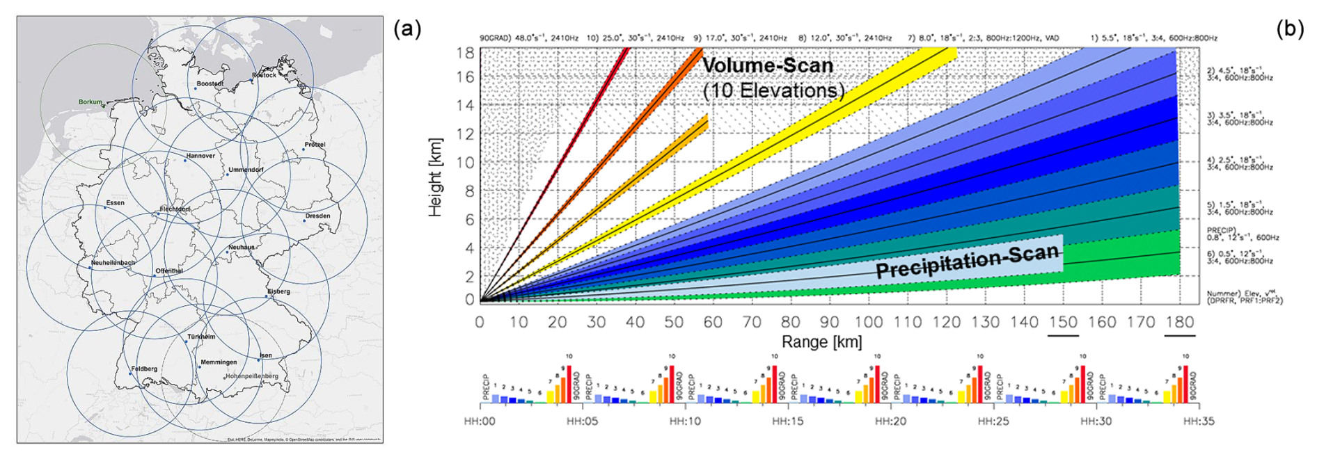
Figure 2 (a) Depiction of the German radar network covering the area of Germany. Each radar station is depicted as an individual circle and has a range of 150 km. (b) Scanning strategy of each radar station of the German radar network. Each of the 10 fixed elevations and the terrain-following precipitation scans are shown.

2.4 Latent heat nudging

The LHN mechanism is a feature of KENDA that enables the assimilation of radar-derived precipitation rates, independent of the assimilation of volume radar data. Note that these precipitation rates are derived from radar data supplied by the OPERA network (including a precipitation scan of the German radar network). For further details on the LHN approach and its integration into KENDA, please refer to Stephan et al. (2008) and Schraff et al. (2016).

3 Targeted covariance inflation

In the following, we discuss the basic elements of the TCI approach, aiming for an improvement in the LETKF assimilation of 3D radar reflectivity data. This approach is motivated by the fact that the LETKF has a fundamental deficit when assimilating observations whose associated simulated ensemble spread vanishes. In numerical applications, such observations are effectively discarded by the LETKF algorithm and have no practical impact on the generated increments, which can also be seen directly through Eqs. (5)–(9). The TCI approach specifically aims to resolve this issue by inflating the ensemble spread for such observations.

We would like to note that the opposite of the previously described scenario – spurious convection in the model background when observations show no convection – is not directly addressed in this study. This issue is generally handled by the standard mechanisms of the LETKF data assimilation and is not related to the ensemble spread problem that the TCI specifically targets.

The spread inflation is achieved by employing a specifically designed model to compute artificially simulated reflectivities for all ensemble members. This model is based on empirically observed correlations found in the nearest spatiotemporal vicinity of convective events. Note that the particular design of the model for the construction of artificial reflectivities is driven by the intention to make the LETKF produce additional increments that make convective initiation and the dynamic generation of reflectivity in the nearest vicinity of spread-inflated observations throughout a subsequent NWP run more likely to occur. See Sect. 3.1 for an in-depth discussion of the construction of this model.

The overall TCI algorithm only computes and assigns artificially simulated reflectivities for observations fulfilling a certain set of conditions. As a consequence, the TCI usually only makes modifications to a very small subset of the most relevant radar observations, and the negative effects (like a potential negative impact on observation error statistics; see Sect. 4.3.1) on the system state are kept at a minimum. See Sect. 3.2 for a discussion of these conditions and a concise formulation of the overall TCI algorithm.

Finally, the TCI algorithm has to be implemented and integrated into the KENDA system to perform the numerical experiments, which is discussed briefly in Sect. 3.3.

3.1 A process-oriented regression model for the TCI

The computation of artificially simulated reflectivities Z of the TCI approach is based on an application of a specifically constructed model ℳ. Considering the general functional form of this model, we assume a linear relationship between the simulated reflectivity perturbation δZ (restricted to heights h above mean sea levels of 3000 to 4000 m) and the simulated specific humidity perturbation δq_v at a certain ICON level L. Formally, this may also be written as follows:

$$\begin{array}{}\text{(10)}& {\displaystyle }{\displaystyle }\mathit{\delta }{Z}^i(\mathit{\lambda },\mathit{\varphi },h)=\mathcal{M}\left(\mathit{\delta }{q_{\mathrm{v}}}^i\right(\mathit{\lambda },\mathit{\varphi },L\left)\right)={\mathit{\alpha }}_L\cdot \mathit{\delta }{q_{\mathrm{v}}}^i(\mathit{\lambda },\mathit{\varphi },L),\end{array}$$

with the ensemble member index i, longitude λ, and latitude ϕ. We would like to point out that, firstly, this model lives within the ensemble perturbation space as only ensemble perturbations δZ and δq_v are used as variables. Secondly, this is a height-based approach; i.e., the algorithm only differentiates between the heights of the radar observations and does not explicitly take the actual radar elevation angle into account.

To determine the coefficients α_L, we perform a linear regression for each available value for the parameter L, i.e., the specific ICON level used for the independent variable q_v. The definite value for the parameter L is then selected by finding the maximum position of the corresponding correlation coefficient ρ_L. As shown in Fig. 3, there is a clear maximum for this correlation coefficient of ρ=0.8  at L=30 (with α=16 000 dB(Z) kg kg⁻¹).

Figure 3 Performing a fit of Eq. (10) to data that are exclusively related to early-stage convective events (see the text for more information on the data preparation steps), this plot depicts the resulting correlation coefficient ρ_L over the ICON level L of the specific humidity variable q_v for each of these fits. To study the effect of spatiotemporal displacements between reflectivities and specific humidities, a moving average with strength β is applied to the 2D input fields for q_v (see Eq. 11).

The dataset used for each linear regression is constructed as follows:

1. All simulated reflectivity data (from all elevation angles of the volume scan) and specific humidity data from all ensemble forecasts are collected. The forecasts provide data every 10 min and start hourly for the first 24 h of an ICON-D2 assimilation cycle with 40 ensemble members. This cycle is initialized at 2019-06-03T00:00:00, which coincides with the beginning of the period studied in Sect. 4.

2. All of the data are interpolated to a regular grid with 2 km resolution.

3. The volume radar data are binned with respect to the height above mean sea level, using bin edges at {1000, 2000, …, 10 000 m}, and the mean value is calculated for all data points within each bin.

A filter is then applied to this initial large dataset to only include data representative of early-stage convective events, i.e., data from spatial and temporal points near newly emerging convective cells. For each assimilation date d₀ and lead time t₀, this filter includes only those horizontal positions (x₀,y₀) in the final dataset that satisfy the following conditions:

1. At time $t=t_{\mathrm{0}}-\mathrm{10}$ min, within a 20 km radius of (x₀,y₀), the ensemble mean of the lowest available radar data bin is below 1 dBZ.

2. At time t=t₀, the ensemble mean of the lowest available radar data bin at (x₀,y₀) is above 10 dBZ.

We found that these specific conditions (based on ensemble mean data) are fairly robust at identifying spatial positions where at least one of the ensemble members is associated with convective initiation and convection in the growing process.

By only including data associated with convective processes, we intend to capture the most relevant correlations associated with convection and, therefore, construct a more process-oriented approach which will eventually be more capable of pulling the system state towards an environment that is likely to initiate convection and help the model dynamically produce reflectivity.

Finally, it is important to note that the algorithm we just discussed for constructing and selecting a TCI model, used to compute artificial reflectivities, is only loosely related to the overall algorithm that applies this selected TCI model based on specific observation selection rules, as discussed in Sect. 3.2. However, as we will demonstrate, both algorithms follow the same general principles and ideas.

3.2 Conditional TCI based on observation and ensemble characteristics

Another important advancement compared to earlier versions of the TCI approach (Vobig et al., 2021) is that multiple specific conditions must be fulfilled before the TCI is applied for a specific observation. We found that this restriction of an application of the TCI to only a small subset of all available observations and, as a consequence, keeping the overall impact on the system state at a minimum is essential for keeping the negative effects of the TCI under control.

Some of the following operations involve the calculation of a moving average acting solely on the two horizontal dimensions. This is implemented as a centered convolution employing a normalized rectangular function of width β (given in kilometers) in both horizontal dimensions λ and ϕ as a kernel. Denoting such a kernel as f_β(λ,ϕ), the processing of an arbitrary field X can be written formally as

$$\begin{array}{}\text{(11)}& \begin{array}{rl}{\stackrel{\mathrm{̃}}{X}}_{\mathit{\beta }}(\mathit{\lambda },\mathit{\varphi },h)& =\underset{-\mathrm{\infty }}{\overset{\mathrm{\infty }}{\int }}\underset{-\mathrm{\infty }}{\overset{\mathrm{\infty }}{\int }}\mathrm{d}{\mathit{\lambda }}^{\prime }\mathrm{d}{\mathit{\varphi }}^{\prime }\\ & f_{\mathit{\beta }}(\mathit{\lambda }-{\mathit{\lambda }}^{\prime },\mathit{\varphi }-{\mathit{\varphi }}^{\prime })X({\mathit{\lambda }}^{\prime },{\mathit{\varphi }}^{\prime },h).\end{array}\end{array}$$

In the following, we employ the Boolean field $\mathcal{B}(\mathit{\lambda },\mathit{\varphi },h)$ to specify, for each spatial position, whether the TCI should be active (where its value is “true” or “1”) and simulated reflectivity values modified or whether the TCI should be inactive (“false” or “0”) and simulated values left unmodified. Furthermore, this field is defined as being the result of a logical conjunction of several auxiliary Boolean fields ${\mathcal{B}}_i(\mathit{\lambda },\mathit{\varphi },h)$:

$$\begin{array}{}\text{(12)}& {\displaystyle }{\displaystyle }\mathcal{B}(\mathit{\lambda },\mathit{\varphi },h)=\prod _i{\mathcal{B}}_i(\mathit{\lambda },\mathit{\varphi },h),\end{array}$$

where each of these Boolean fields ${\mathcal{B}}_i(\mathit{\lambda },\mathit{\varphi },h)$ is the result of an individual condition check.

$$\begin{array}{}\text{(13)}& {\displaystyle }\begin{array}{rl}& \text{Spread check:}\\ & {\mathcal{B}}_{\mathrm{1}}(\mathit{\lambda },\mathit{\varphi },h)\equiv \left\{\begin{array}{ll}\mathrm{1}& \text{if }{\mathit{\sigma }}_i\left[Z^{\left(i\right)}\right(\mathit{\lambda },\mathit{\varphi },h\left)\right]<\text{0.1\hspace{0.17em}dB(Z)},\\ \mathrm{0}& \text{otherwise.}\end{array}\right.\end{array}\text{(14)}& {\displaystyle }\begin{array}{rl}& \text{Deterministic check:}\\ & {\mathcal{B}}_{\mathrm{2}}(\mathit{\lambda },\mathit{\varphi },h)\equiv \left\{\begin{array}{ll}\mathrm{1}& \text{if }{\stackrel{\mathrm{̃}}{Z}}_{\mathit{\beta }=\mathrm{10}}^{\det }(\mathit{\lambda },\mathit{\varphi },h)<\text{1\hspace{0.17em}dBZ},\\ \mathrm{0}& \text{otherwise.}\end{array}\right.\end{array}\text{(15)}& {\displaystyle }\begin{array}{rl}& \text{Ensemble mean check:}\\ & {\mathcal{B}}_{\mathrm{3}}(\mathit{\lambda },\mathit{\varphi },h)\equiv \left\{\begin{array}{ll}\mathrm{1}& \text{if }{\mathit{\mu }}_i\left[{\stackrel{\mathrm{̃}}{Z}}_{\mathit{\beta }=\mathrm{10}}^{\left(i\right)}\right(\mathit{\lambda },\mathit{\varphi },h\left)\right]<\text{1\hspace{0.17em}dBZ},\\ \mathrm{0}& \text{otherwise.}\end{array}\right.\end{array}\text{(16)}& {\displaystyle }\begin{array}{rl}& \text{Observation check:}\\ & {\mathcal{B}}_{\mathrm{4}}(\mathit{\lambda },\mathit{\varphi },h)\equiv \left\{\begin{array}{ll}\mathrm{1}& \text{if }{Z}^{\mathrm{obs}}(\mathit{\lambda },\mathit{\varphi },h)]>\text{15\hspace{0.17em}dBZ},\\ \mathrm{0}& \text{otherwise.}\end{array}\right.\end{array}\text{(17)}& {\displaystyle }\begin{array}{rl}& \text{Height check:}\\ & {\mathcal{B}}_{\mathrm{5}}(\mathit{\lambda },\mathit{\varphi },h)\equiv \left\{\begin{array}{ll}\mathrm{1}& \text{if }\text{3000\hspace{0.17em}m}\le h\le \text{4000\hspace{0.17em}m},\\ \mathrm{0}& \text{otherwise.}\end{array}\right.\end{array}\end{array}$$

Note that we employ σ_i[X⁽ⁱ⁾] and μ_i[X⁽ⁱ⁾] to denote the spread and mean, respectively, of a variable X.

With ℬ₁, we ensure that we only make changes for observations whose associated ensemble spread is too small. The fields ℬ₂, ℬ₃, and ℬ₄ ensure that the deterministic member and the ensemble mean have to vanish, while, simultaneously, there has to be a sizable observed reflectivity; i.e., there has to be a large discrepancy between observed and simulated values. Note that the calculation of ℬ₂ and ℬ₃ relies on simulated fields that have been preprocessed by means of a moving average (defined in Eq. 11). This is done to take possible spatiotemporal displacements between observed and simulated reflectivity cells into account. Finally, ℬ₅ ensures that the TCI is only applied for radar observations whose heights fall within a certain height range. This is important as the previously constructed TCI model (see Sect. 3.1) is based on observations falling within this specific height range.

We conducted sensitivity tests on the parameters in Eqs. (13)–(17), varying them within a defined range to assess their impact on DA performance and short-term NWP forecasts. The results showed that small changes had minimal impact, and the final parameters were chosen to balance effective TCI application while minimizing noise.

The TCI modifies the simulated reflectivity of all ensemble members employing the linear model ℳ (see Eq. 10) defined in Sect. 3.1, but only for a specific subset of all observations which is specified by means of the logical field ℬ. Formally, the inflated reflectivities ${Z^{\prime }}^{\left(i\right)}$ of the ith ensemble member are then computed via the following rule:

$$\begin{array}{}\text{(18)}& \begin{array}{rl}& {Z^{\prime }}^{\left(i\right)}(\mathit{\lambda },\mathit{\varphi },h)=\\ & \left\{\begin{array}{l}{\mathit{\mu }}_i\left[Z^{\left(i\right)}\right(\mathit{\lambda },\mathit{\varphi },h\left)\right]\\ +\mathcal{M}\left({\stackrel{\mathrm{̃}}{\mathit{\delta }{q}_{\mathrm{v}}}}_{\mathit{\beta }=\mathrm{10}}^{\left(i\right)}(\mathit{\lambda },\mathit{\varphi },l=\mathrm{30})\right)& \text{if }\mathcal{B}(\mathit{\lambda },\mathit{\varphi },h)\text{ is true,}\\ Z^{\left(i\right)}(\mathit{\lambda },\mathit{\varphi },h)& \text{otherwise}.\end{array}\right.\end{array}\end{array}$$

λ, ϕ, and h loop over all discrete spatial points for which a reflectivity is measured. Note that in Eq. (18) the field for q_v that enters the TCI algorithm is preprocessed by means of a moving average for taking spatiotemporal displacements into account.

Overall, Eqs. (18) and (10) demonstrate that reflectivity perturbations are derived deterministically from specific humidity perturbations using a linear model – without the involvement of any random perturbations – and are then applied conditionally.

Additionally, we modify the observation error for each observation for which the ensemble is inflated. Usually, we use a global observation error of 10 dB(Z) for all radar observations in our quasi-operational setup. However, if the TCI is applied for a specific observation $Z^{\mathrm{obs}}(\mathit{\lambda },\mathit{\varphi },h)$, which means that $\mathcal{B}(\mathit{\lambda },\mathit{\varphi },h)$ is true, the observation error is reduced to 2 dB(Z). This results in much more pronounced increments, and the system is pulled significantly more strongly towards these observations.

Note that we performed the same sensitivity checks on the reflectivity observation error as in our previous TCI study (Vobig et al., 2021), and the results were consistent. These findings confirm that the observation error significantly influences the size of the increments, underscoring its importance in the TCI process. The chosen value for the observation error of 2 dB(Z) strikes a balance, ensuring that no excessively large increments are introduced while maintaining the effectiveness of the TCI application.

3.3 Implementation

To integrate the TCI approach into the KENDA system (see Sect. 2.1), the input data that eventually enter the LETKF system are preprocessed. Usually, these input data are supplied in the form of feedback files (containing all superobbed² reflectivity observations and model equivalents to be assimilated) and model field files (containing, e.g., the model fields for q_v), where there is one file per ensemble member and radar station. Processing each radar station and radar elevation separately, the TCI is implemented by performing the following steps sequentially:

1. Read all required ICON q_v model fields for all ensemble members from the model field files.

2. Read all required observed and simulated radar reflectivity data Z for all ensemble members and all radar stations from the radar feedback files.

3. Interpolate Z and q_v onto a common regular 2D horizontal grid (using a resolution of 2 km).

4. Construct the logical field ℬ; see Eq. (12).

5. Calculate modified simulated reflectivities for all ensemble members using the TCI algorithm; see Eq. (18).

6. Write modified simulated reflectivities back to their corresponding radar feedback files. This step involves an inverse map from the regular grid used internally by the TCI algorithm to the irregular grid used internally by the radar feedback files.

7. Modify observation errors (within the radar feedback files) for observations whose related ensemble spread was inflated.

Based on the observations and model equivalents, the LETKF calculates a transform vector for the mean and a transform matrix for the ensemble perturbations (i.e., the ensemble where its mean is subtracted), which are applied to the first-guess ensemble to calculate the analysis ensemble. In the KENDA (Schraff et al., 2016) implementation, the calculations of the model equivalents are carried out during the model run and are saved in the so-called feedback files. The calculation of the transform matrices and the execution of the transform are performed in a subsequent step by the core KENDA module.

4 Numerical results

4.1 Case study setup

To study the effects of the TCI, we performed data assimilation cycles for ICON-D2 over the period from 2019-06-03T00:00 to 2019-06-20T00:00 at an hourly data assimilation frequency. This specific time frame extends for several days for which individual case studies have been selected by the RealPEP (Near-Realtime Quantitative Precipitation Estimation and Prediction) research group. It includes many typical convective events. The general meteorological situation and its temporal development over the course of the chosen time period are shown in Fig. 4 by means of the spatial fraction of reflectivities above a certain threshold of time.

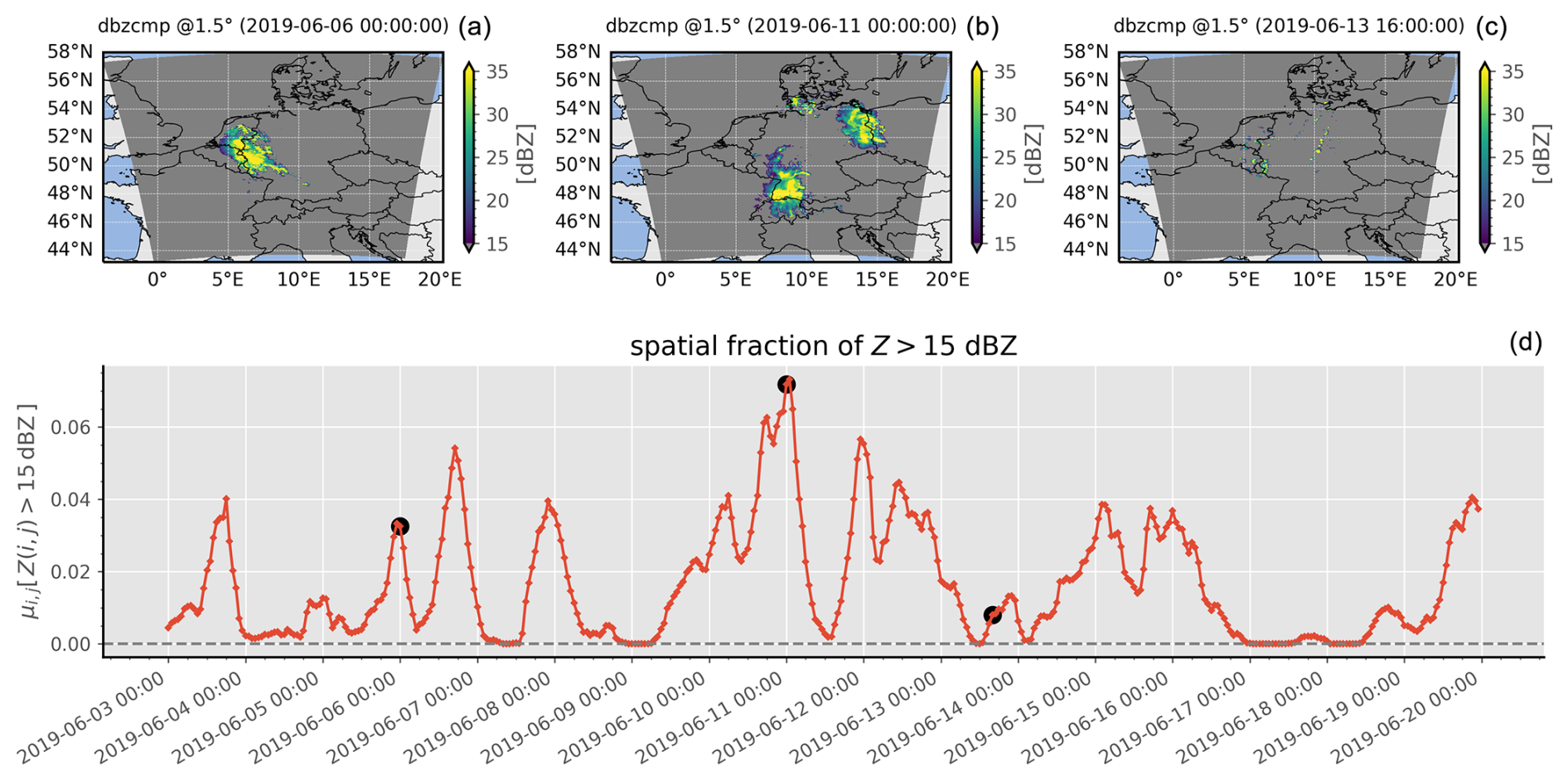
Figure 4 Using all available radar observations from the radar composite at 1.5°, panel (d) depicts the fraction of all radar reflectivities whose value is above the threshold of 15 dBZ over time. For three exemplary points in time that are also indicated by the black circles in panel (d), panels (a), (b), and (c) show the associated radar reflectivity composites.

To study the intrinsic effects of the TCI approach, we performed two assimilation cycles³: a reference cycle and a TCI cycle, which differ from each other solely by the fact that the TCI is either inactive or active. The TCI cycle applies the TCI algorithm at each assimilation step, i.e., hourly to all radar data entering the LETKF assimilation algorithm. For both assimilation cycles, we performed free forecasts every 3 h with a 6 h lead time. During these forecasts, no assimilation and, therefore, no TCI take place.

Overall, the configuration of these two assimilation cycles is basically the operational configuration. This includes the assimilation of all conventional data, the assimilation of 3D radar data from the German radar network, the assimilation of radar data obtained from radar precipitation scans via the LHN mechanism, and the usage of an ensemble of 40 members. In contrast to the operational assimilation, we did not include the all-sky assimilation of satellite data in our experiments, since the operationalization of these was carried out during the project execution.

At each data assimilation step, the LETKF generates increments for several model variables, particularly for the temperature T and the specific humidity q_v, which by incremental analysis update (IAU) (Bloom et al., 1996) are fed into the system propagation throughout a certain time window centered around the assimilation time. However, it is important to note that, for our operational setup, there are no increments for hydrometeors other than q_v, e.g., q_r, q_i, and q_c.

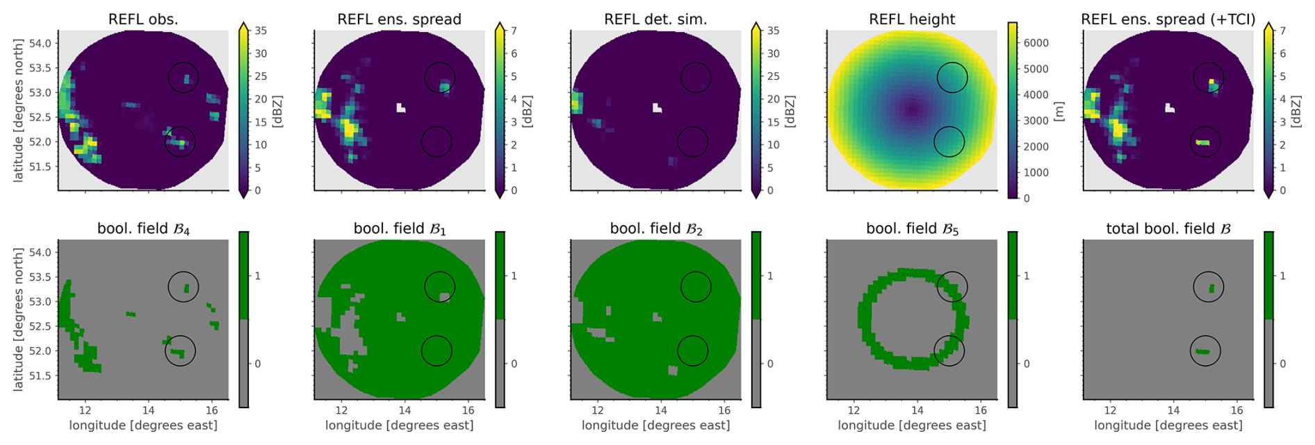
Figure 5 Illustration of the Boolean fields ℬ_i and their associated input fields, the total field ℬ, and the resulting inflated reflectivities (see Eqs. 12–18) at t₀=2019-06-05T15:00:00. Note that radar reflectivity data of one single radar station (Prötzel) at one single radar elevation angle of 1.5° only are employed here. Each of the first four columns is related to a certain necessary condition of the TCI and depicts the result of the computation of a certain ℬ_i field (bottom row) together with its related input fields (top row). The last column shows the total field ℬ resulting from a logical conjunction of all ℬ_i (bottom row) and the computed reflectivity ensemble spread after the TCI has been applied to all of the members (top row).

4.2 Study of individual cases

Let us now look more closely at the TCI effects by exemplarily studying the details of an assimilation at t₀=2019-06-05T15:00:00 and its impact on a subsequent model run up to 1 h after t₀.

Let us begin with an illustration of certain internal details and immediate effects of the TCI algorithm, in particular the construction of the total Boolean field ℬ and the computation of the final inflated reflectivities (see Sect. 3.2 for more information). For this purpose, Fig. 5 depicts selected ℬ_i fields as well as their corresponding input fields, the total Boolean field ℬ, and the final inflated reflectivities obtained from the TCI. Note that here we only visualize the radar data of one exemplarily chosen radar station at a single radar elevation angle to improve the clarity of this illustration.

Two things become apparent here: firstly, there are only very few spatially connected regions for which ℬ is true, and, secondly, the TCI is successfully able to increase the reflectivity ensemble spread within these regions. Directly related to Fig. 5, an aggregation (taking the mean) over all of the radar stations and all of the elevation angles of the Boolean field ℬ and difference in the ensemble spread is depicted in Fig. 6, allowing an overview of the complete model domain. Similarly to before, it becomes evident that there are only very few spatially connected regions within the complete domain that are compatible with the imposed conditions for an application of the TCI. Looking at the depicted difference between the reflectivity ensemble spread with and without the TCI, it also becomes directly clear that the TCI is able to increase the reflectivity ensemble spread if ℬ is true. However, the ensemble spread is always kept unmodified for observations for which ℬ is false.

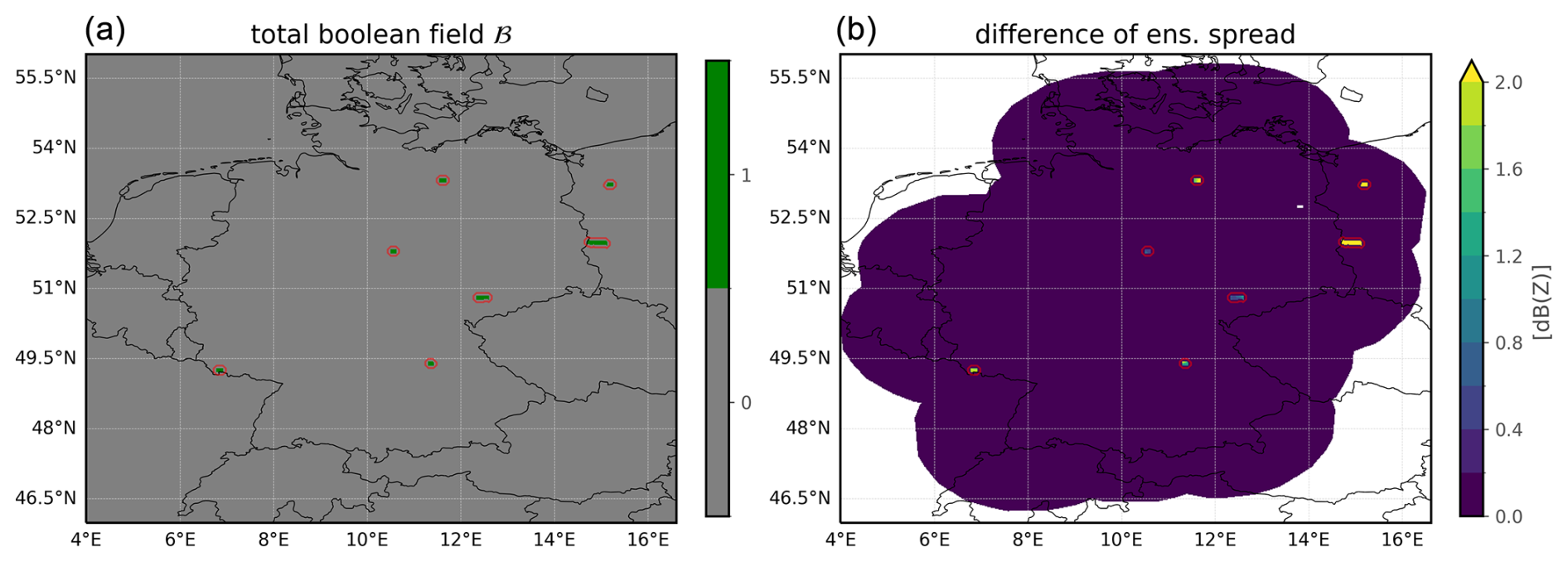
Figure 6 Depiction of the total Boolean field ℬ (a) and the difference in the reflectivity ensemble spread with and without the TCI (b) at t₀=2019-06-05T15:00:00. While this figure is closely related to Fig. 5, the 2D fields shown here are the result of an aggregation (taking the mean) over all available radar stations and radar elevation angles, allowing for an overview of the complete model domain. Red contours are used here to indicate regions for which the aggregated Boolean field ℬ is true, i.e., areas for which the TCI algorithm is potentially active.

As the TCI increases the spread by modifying all ensemble members of only a few carefully selected observations for which the spread would be vanishing otherwise, we enable the LETKF to include these otherwise discarded observations. This leads to altered increments that are produced by the LETKF, and we expect these increments to modify our system in a way that makes the generation of reflectivity more likely. It is important to note that, firstly, reflectivity is not a prognostic variable but merely a diagnostic variable, and, secondly, we are not updating hydrometeor variables that are directly connected to the simulation of reflectivity (e.g., q_r). Therefore, increments do not directly affect reflectivities, but the model has to respond dynamically to increments for other variables, e.g., temperature and specific humidity, and it may eventually, after a short period of time, dynamically generate reflectivity through the generation of, e.g., q_r and q_g.

To observe how the TCI is able to let new reflectivity cells emerge, let us consider Fig. 7. By considering the depicted reflectivity composite at a lead time of 1 h, it becomes clear that the TCI is very often able to produce new simulated reflectivity cells that are consistent with observed reflectivity cells and that are not produced (or at least are not as pronounced) without application of the TCI. Thus, we can already observe a positive impact of the TCI here.

It is important to note that Fig. 7 illustrates the general trend observed for other assimilation dates and lead times that are not shown. For regions in which the TCI is active, the simulation of the TCI cycle is very often able to produce new reflectivities that are not present in the reference cycle. However, for very large observed values, the corresponding simulated values of the TCI cycle are usually smaller than the observed ones – which is, however, plausible as the model had only 1 h here to dynamically respond to the additional increments introduced by the TCI and the production of reflectivity. Note that two other possible explanations for this general trend are that the TCI is only applied over a small height range of 3 to 4 km, limiting the region that can be convectively destabilized, and that the relatively sluggish model begins its convection later than in reality, preventing it from evolving as quickly.

Furthermore, we would like to note that the source of possible differences between the two simulated reflectivity composites may be two-fold: firstly, the TCI has an effect through the very last assimilation step, and, secondly, the TCI has also been applied hourly at many assimilation steps before the very last one at t₀, such that there is also an accumulation of its effects and, therefore, a substantial divergence of the background states of the TCI and the reference cycle at t₀.

The direct impact of the TCI on convective initiation (without any possible accumulation effects) was investigated in Vobig et al. (2021), where the TCI was applied at single time steps in the context of non-cycled experiments. These “cold-start scenarios” demonstrated that the TCI is effective even when applied only once. In the current study, we confirmed that the TCI produces similar results in cold-start scenarios, generating reflectivity even when applied at a single time step instead of through cycling.

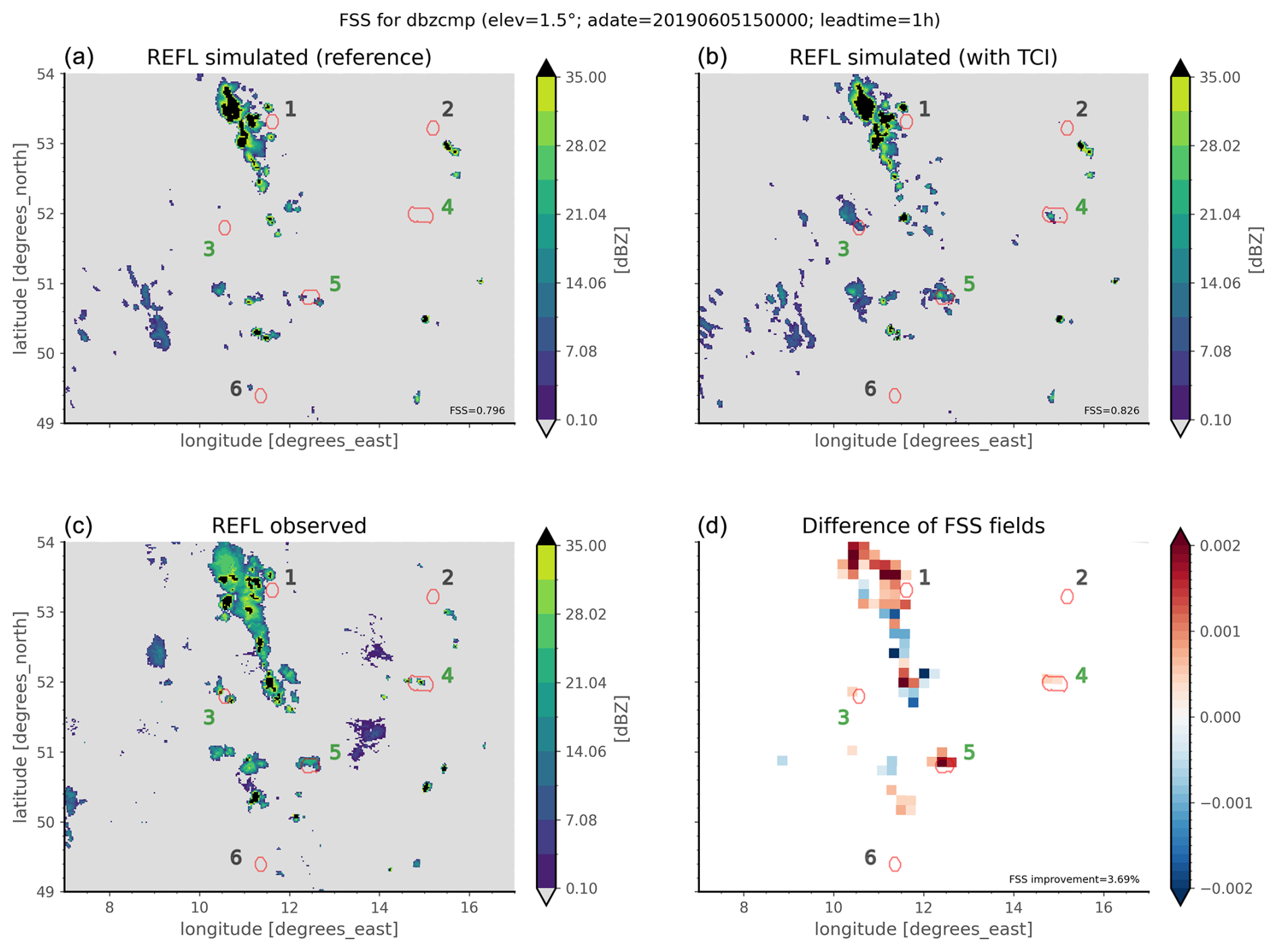
Figure 7 Visualization of radar reflectivity composites at 1.5 ° for the observed values (c), simulated values of the reference assimilation cycle (a), and simulated values of the TCI assimilation cycle (b). The lead time here is 60 min with respect to the last assimilation at t₀=2019-06-05T15:00:00. Panel (d) shows the field Δfss computed from reflectivity data of the other three panels for β=20 km and τ=15 dBZ (see Eqs. 19 and 20). Similar to Fig. 6, the red contours in all four plots indicate regions for which the TCI was active during the last assimilation at t₀. Each red contour is also assigned a number for better visibility and identification, and, additionally, the color of each number indicates whether there is an overall positive (green) or neutral (gray) impact of the TCI on the related region.

Let us now further formalize and quantify the verification of reflectivities at a single time step as shown in Fig. 7 by employing a special version of the FSS designed by Roberts and Lean (2008) to deal with highly structured fields such as reflectivity that are particularly susceptible to double penalties (Rossa et al., 2008).

The FSS is a popular spatial verification metric that is also used in this work for the spatial verification of reflectivities for longer-term experiments in Sect. 4.3 and, thus, it is particularly important for the overall evaluation of the TCI approach. We denote 2D fields for observations and associated predictions as Y(i,j) and X(i,j), respectively, where i and j are indices for the two horizontal dimensions. Considering an arbitrary 2D field A(i,j), we use the notation ${\widehat{A}}_{\mathit{\beta },\mathit{\tau }}(i,j)$ to refer to the so-called fraction-of-occurrences field. The fraction-of-occurrences field is defined for each spatial point as the fraction of spatial points whose value is above the threshold τ with respect to all spatial points lying within a certain spatial neighborhood around this point – defined by a 2D box with box length β. The FSS with respect to these two input fields X and Y, the box length β, and the dBZ threshold τ may now be written as follows:

$$\begin{array}{}\text{(19)}& {\mathrm{\text{FSS}}}_{X,Y,\mathit{\beta },\mathit{\tau }}=\mathrm{1}-\sum _{i,j}{\displaystyle \frac{{\left({\widehat{X}}_{\mathit{\beta },\mathit{\tau }}(i,j)-{\widehat{Y}}_{\mathit{\beta },\mathit{\tau }}(i,j)\right)}^{\mathrm{2}}}{{\sum }_{k,l}{\widehat{X}}_{\mathit{\beta },\mathit{\tau }}(k,l{)}^{\mathrm{2}}+{\sum }_{k,l}{\widehat{Y}}_{\mathit{\beta },\mathit{\tau }}(k,l{)}^{\mathrm{2}}}}.\end{array}$$

By comparing two different predictions X and X^′ by means of the difference of their corresponding FSS values with each other, we obtain

$$\begin{array}{}\text{(20)}& {\displaystyle }{\text{FSS}}_{X^{\prime },Y,\mathit{\beta },\mathit{\tau }}-{\text{FSS}}_{X,Y,\mathit{\beta },\mathit{\tau }}=\sum _{i,j}\mathrm{\Delta }{\text{fss}}_{X^{\prime },X,Y,\mathit{\beta },\mathit{\tau }}(i,j),\end{array}$$

where we inserted Eq. (19), combined both sums in the resulting expression, and then implicitly defined the 2D field $\mathrm{\Delta }{\text{fss}}_{X^{\prime },X,Y,\mathit{\beta },\mathit{\tau }}(i,j)$ as the argument of this combined sum. Evidently, from the sign and magnitude of $\mathrm{\Delta }{\text{fss}}_{X^{\prime },X,Y,\mathit{\beta },\mathit{\tau }}(i,j)$, we may assess how much the prediction $X^{\prime }(i,j)$ improves (positive values) or worsens (negative values) the overall FSS with respect to the reference prediction X(i,j) and observation Y(i,j).

Following these considerations, Fig. 7d shows the aforementioned 2D field $\mathrm{\Delta }{\text{fss}}_{X^{\prime },X,Y,\mathit{\beta },\mathit{\tau }}(i,j)$ based on simulated reflectivities of the TCI cycle for X^′, simulated reflectivities of the reference cycle for X, observed reflectivities for Y, β=20 km, and τ=15 dBZ. Observing that most of the values are positive, it becomes evident that the TCI is predominantly improving the FSS. This qualitative first impression is confirmed by computing the FSS related to the reference cycle reflectivity composite and the FSS related to the TCI cycle reflectivity composite, which amount to 0.796 and 0.826, respectively. Therefore, we obtain a relative improvement in the FSS of the TCI cycle of about 3.69 %.⁴

Interestingly, Fig. 7 demonstrates that the TCI improves reflectivity not only in the near vicinity of regions for which the TCI is applied in the very last assimilation step (indicated by the red contours), but also for many other spatial regions, hinting at an accumulated impact of the TCI on the background state dating back to assimilation steps before the very last one.

4.3 Statistical evaluation of long-term experiments

Let us now proceed to a more statistical view of the TCI effects by studying different statistics and scores of longer-term NWP experiments covering a period of about 17 d. Note that the specific configuration of these experiments, including the setup of their assimilation cycles and free forecasts, was already discussed in Sect. 4.1.

4.3.1 Observation error statistics

Figure 8 shows selected observation error statistics for the TEMP⁵ relative humidity, TEMP temperature, and radar reflectivities. It becomes evident that there is a slight negative impact of the TCI on the mean error of TEMP relative humidity with respect to both the analysis and the first guess, especially at heights around 500 to 600 hPa, which can be interpreted as the TCI introducing additional humidity into the simulation at those heights. However, this kind of impact is – at least to some extent – to be expected and does not necessarily have to be regarded as a negative effect. Considering that the TCI modifies reflectivities only within a certain height range (see Sect. 3.2 and Eq. 17) and employs an algorithm that is based on correlations with the specific humidity at a certain ICON level (see Sect. 3.1), it is plausible that – by taking cross-correlations into account – the LETKF pulls the ensemble mean towards those ensemble members with more specific humidity. Therefore, the LETKF increases the specific humidity of the ensemble mean and the deterministic member but – taking vertical localization into account – only within a certain height band. Considering the root-mean-square error (RMSE) of TEMP relative humidity, only a very small and negligible impact of the TCI becomes evident.

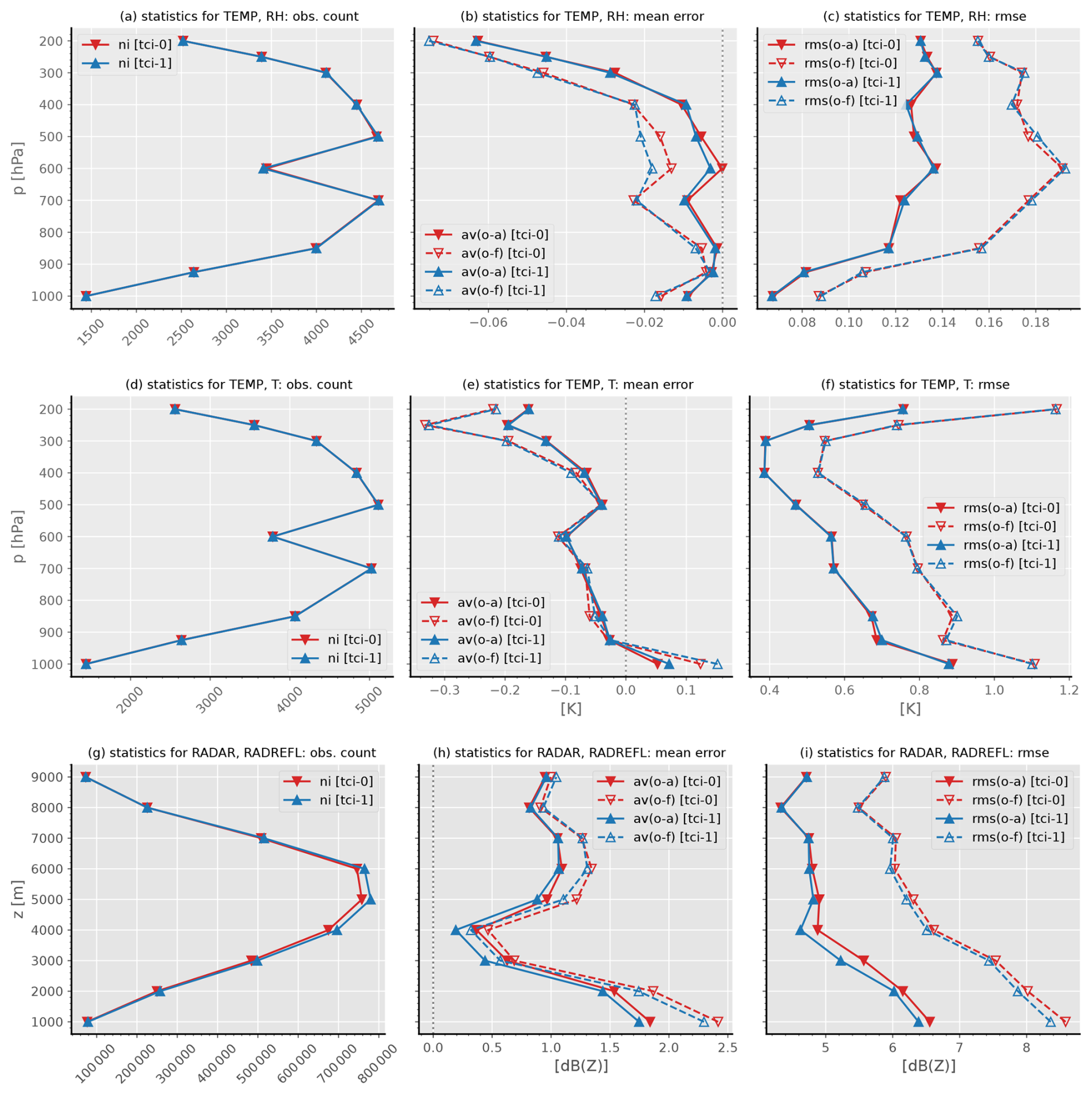
Figure 8 Observation error statistics for the TCI (label “tci-1”) and the reference (label “tci-0”) assimilation cycle over a period from 2019-06-03T00:00 to 2019-06-20T00:00. From top to bottom, statistics for the different observation types TEMP relative humidity, TEMP temperature, and radar reflectivity are shown. From left to right, the number of observations, mean error, and root-mean-square error (RMSE) are depicted. Note that the mean error and RMSE statistics are based on the difference of observations with their corresponding first-guess values (“o-f” included in the label) or analysis values (“o-a” included in the label).

To better understand the additional humidity bias introduced by the TCI, we examined the mean error of TEMP relative humidities on an hourly basis rather than aggregating over the entire study period. Our findings reveal that the additional humidity bias does not simply increase over time and saturate after a certain number of TCI applications. Instead, it fluctuates erratically, alternating between negative and positive values on an hourly scale. One possible explanation for this behavior is that any TCI effect on simulated relative humidities contributing to these statistics likely already evolved through space and time and is influenced by the model's highly nonlinear dynamics, given that it is statistically uncommon for the locations where the TCI is applied to overlap with those where TEMP measurements are taken. Additionally, it is worth noting that the ensemble spread and spread–skill ratio of relative humidity remain practically unchanged upon the application of the TCI.

Similar to TEMP relative humidity, the TCI has a slight effect on the mean error of TEMP temperature, which can be interpreted as the TCI increasing the temperature, especially near the ground at lower altitudes. The RMSE of TEMP temperature, however, does not exhibit any relevant effects of the TCI.

Finally, it is demonstrated that both the mean error and the RMSE of radar reflectivities are reduced through the TCI.

Overall, the largest negative impact of the TCI on observation error statistics is seen for the mean error of TEMP relative humidity. However, the magnitude of this effect is still acceptable and for the most part is to be expected. Note that a major problem of a further advancement of an earlier version of our TCI approach as presented in Vobig et al. (2021) was – when applied to all radar and not employed within a single-observation context – a significant negative impact on observation error statistics, especially on the statistics for TEMP relative humidity. The reduction of this negative impact – while still maintaining the positive effects of the TCI – was therefore one of the main objectives that decisively guided the further advancement of the TCI towards the current version presented in this work.

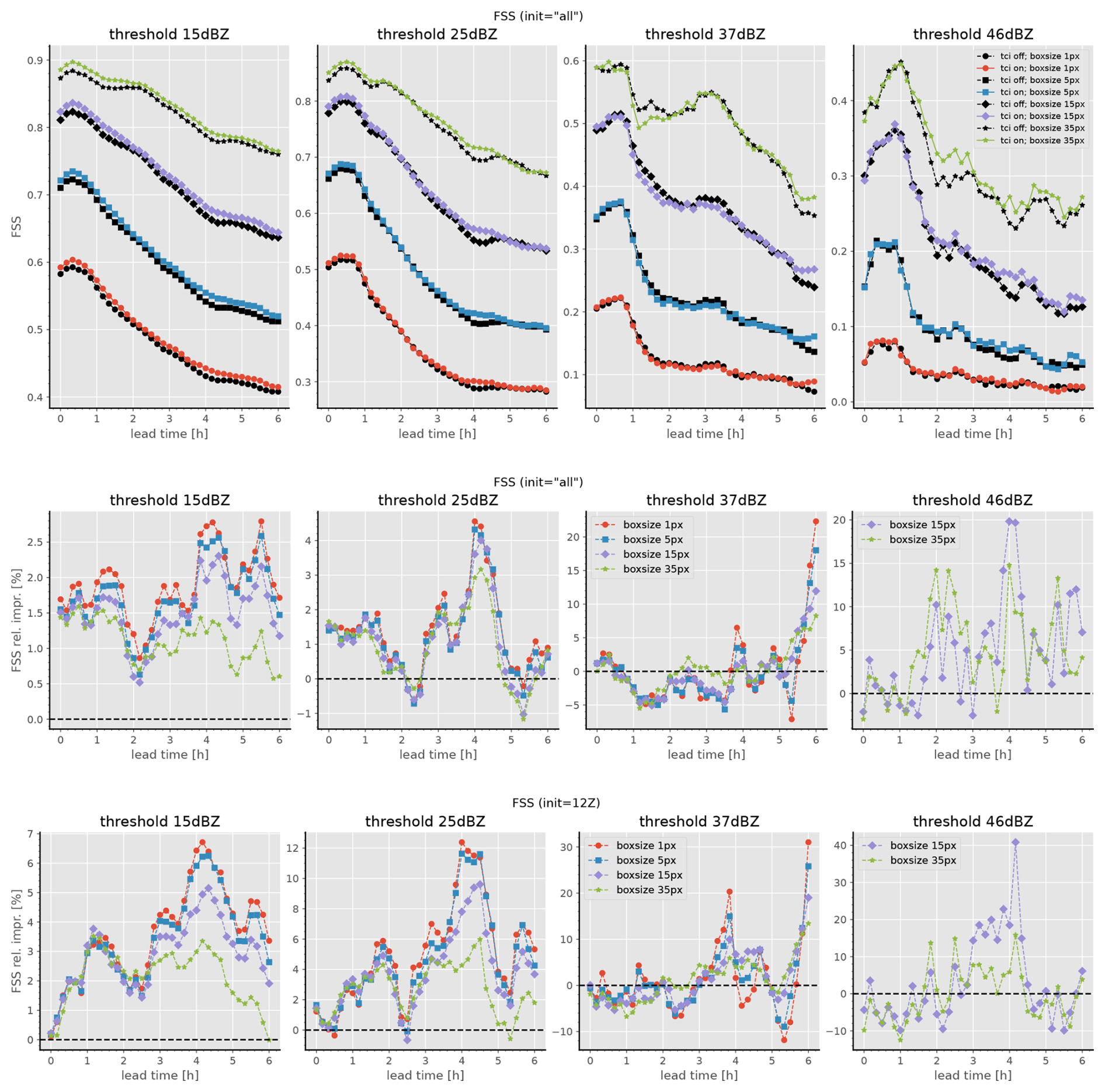
Figure 9 Fractional skill score (FSS) of reflectivity composites of free forecasts over lead times. The FSS calculation is based on forecasts branching off the TCI assimilation cycle (label “tci on”) or the reference assimilation cycle (label “tci off”). For further details on the setup of this case study over the period of more than 2 weeks, see Sect. 4.1. Each panel within the upper row depicts the FSS for both experiments. Directly related to the upper row, the middle row depicts the relative FSS improvement (in percent) of the “tci on” experiment with respect to the “tci off” experiment. Similar to the middle row, the bottom row also depicts the relative FSS improvement but exclusively employs data from free forecasts starting at 12:00 UTC. For all of the rows, the threshold used for the FSS calculation is varied column-wise, and each panel shows results for several box sizes (given in pixels, where 1 pixel amounts to 2.2 km).

4.3.2 Fractional skill score

The positive impact of the TCI is demonstrated by means of Fig. 9, which depicts the FSS of radar reflectivity composites of free forecasts with respect to their lead times.⁶ It should be noted that this verification is conducted with respect to the complete model domain and not only for regions for which the TCI has been active. Furthermore, the following analysis is based on full-scale data assimilation and forecasting experiments covering a period of more than 2 weeks and employing a quasi-operational configuration – which especially includes an active LHN mechanism – as already discussed in Sect. 4.1.

Let us begin our analysis with the top and middle rows of Fig. 9, depicting FSS statistics based on the reflectivity data of all available free forecasts; i.e., there are no further restrictions on the initialization times of these forecasts. Regarding the threshold 15 dBZ, it becomes evident that the TCI consistently improves the FSS for all of the depicted box lengths and lead times. It is especially remarkable that this positive effect is still clearly visible even after 6 h. The positive effect of the TCI on the FSS tends to decrease with box length, and the relative improvement amounts to up to 2.7 % for the box length of 1 pixel and up to 1.6 % for the longest box length of 35 pixels. Considering the plots for the threshold of 25 dBZ, a similar conclusion to before can be drawn; i.e., a positive impact of the TCI is clearly visible and amounts to up to 4.3 % for the box length of 1 pixel. Regarding the two largest thresholds of 37 and 46 dBZ, the curves of the FSS with respect to the lead time become more erratic. However, the overall effect (averaged over the lead times) of the TCI still ranges from neutral to clearly positive when taking all of the lead times into account.

Furthermore, the bottom row of Fig. 9 depicts fractional skill score improvements based solely on radar reflectivity data of model runs initialized at 12:00 UTC, i.e., forecasts for the time frame between 12:00 and 18:00 UTC. During these afternoon hours⁷, the positive effect of the TCI on the FSS is even more pronounced: for the threshold of 15 dBZ, the FSS is improved by up to about 6 %, and for the threshold of 25 dBZ there is even an improvement by up to about 10 %. Consistent with our previous findings, the FSS for the 37 and 46 dBZ thresholds is rather erratic with respect to the lead time. However, when considering all lead times, the overall averaged effect ranges from neutral to clearly positive, with occasional improvements of up to 20 %.

A possible explanation for the more consistent improvement in the TCI at the two lower thresholds of 15 and 25 dBZ, compared to the two higher thresholds, is that higher reflectivities are simply much rarer. Additionally, we generally observe in our NWP system that the LHN mechanism already generates most of the high-reflectivity cells and that, statistically, our current NWP system tends to simulate too many large reflectivities and too few small ones. Given that the TCI can only add reflectivity at each assimilation step and reducing reflectivity requires indirect accumulation effects (i.e., longer-term changes to the background system state), it is also plausible that the TCI is better at improving the representation of the lower-reflectivity band than that of the higher-reflectivity one.

Overall, Fig. 9 demonstrates a clear positive impact of the TCI on the FSS of radar reflectivity composites of up to 10 %. The fact that this effect is still apparent even after 6 h hints at a more profound influence of the TCI on the background system state accumulated throughout several assimilations – which is also consistent with some of the conclusions already drawn in Sect. 4.2.

5 Summary and outlook

We have introduced and studied new process-oriented and conditional approaches to targeted covariance inflation (TCI). For particular cases as well as for full-scale data assimilation and forecasting experiments over a period of more than 2 weeks, we have shown that the approaches can improve the representation of convective processes in the forecasts and lead to clearly improved fractional skill scores for radar reflectivity of up to 10 %.

Details of the evaluation for different dBZ thresholds show that the TCI successfully initializes convection in the range of 15 dBZ to 25 dBZ and also has a positive effect on stronger precipitation cells which form part of the 37 and 46 dBZ threshold scores. The TCI as implemented through Eqs. (10) and (18) is currently not dependent on the strength of the observed reflectivity, though the LETKF will of course use the difference between observed and simulated reflectivities when calculating its increments.

Looking into refinement of the scheme to further improve scores for all reflectivity bands and lead times will be a topic of future research. The sophisticated interplay of convective processes with the broader atmospheric state has the potential to be taken into account in a much deeper way. Here, machine learning (ML) techniques provide a set of very flexible nonlinear tools which can help to model more sophisticated dependencies and use them to develop an AI- or ML-based TCI.

The approach to construct appropriate targeted covariances in an ensemble Kalman filter is very generic and could also be employed in other types of observations. It can also be applied to other ensemble data assimilation methods such as ensemble-variational data assimilation (EnVAR) (Buehner et al., 2013; Meng et al., 2019), where the observation-based covariance matrix enters the scheme in the form of $HB{H}^T=HX{X}^T{H}^T=Y{Y}^T$ or the localized adaptive particle filter (LAPF) (Potthast et al., 2019; Schenk et al., 2022).