A range of outcomes: the combined effects of internal variability and anthropogenic forcing on regional climate trends over Europe

Disentangling the effects of internal variability and anthropogenic forcing on regional climate trends remains a key challenge with far-reaching implications. Due to its largely unpredictable nature on timescales longer than a decade, internal climate variability limits the accuracy of climate model projections, introduces challenges in attributing past climate changes, and complicates climate model evaluation. Here, we highlight recent advances in climate modeling and physical understanding that have led to novel insights about these key issues. In particular, we synthesize new findings from large-ensemble simulations with Earth system models, observational large ensembles, and dynamical adjustment methodologies, with a focus on European climate.

1 Introduction

1.1 Internal variability and forced climate change

The climate system is highly variable in both space and time. This variability originates from processes within the coupled ocean–atmosphere–cryosphere–land–biosphere system and from external influences such as solar and orbital cycles, volcanic eruptions, and anthropogenic emissions of greenhouse gases and sulfate aerosols. A primary source of internally generated variability is the atmospheric general circulation, which produces familiar day-to-day and week-to-week weather fluctuations. The non-linear nature of atmospheric dynamics limits predictability to less than a few weeks; beyond this timescale, atmospheric motions may be considered to be random stochastic processes, often termed “weather noise” (e.g., Lorenz, 1963; Leith, 1973; James and James, 1992). It is important to note that such weather noise imparts variability on a continuum of timescales, from sub-monthly to decadal and longer (e.g., Madden, 1975; Deser et al., 2012; Thompson et al., 2015).

Another important source of internally generated variability is the coupling between the ocean and atmosphere. Large-scale air–sea interactions give rise to distinctive patterns (or “modes”) of variability on interannual and longer timescales, including phenomena such as the El Niño–Southern Oscillation (ENSO; Wang et al., 2017), Pacific decadal variability (PDV; Newman et al., 2016), and Atlantic multi-decadal variability (AMV; Zhang et al., 2019). Like the atmospheric general circulation, these coupled modes are governed by non-linear dynamical processes which limit their predictability. For example, forecast skill is generally limited to 1–2 years for ENSO (Jin et al., 2008; DiNezio et al., 2017; Wu et al., 2021), 5 years for PDV (Teng and Branstator, 2011; Meehl et al., 2016; Gordon and Barnes, 2022), and 10 years for AMV (Griffies and Bryan, 1997; Trenary and DelSole, 2016; Yeager et al., 2018). Beyond these predictability time horizons, internally generated variability can be thought of as a roll of the dice, introducing unavoidable uncertainty to climate model projections, especially at local and regional scales (e.g., Deser et al., 2012, 2014, 2020a).

Not only does the unpredictable internal variability cause irreducible uncertainty in future climate projections, but it also confounds interpretation of the historical climate record. For example, internal variability may partially obscure the regional climate response to external forcings including industrial greenhouse gas emissions, stratospheric ozone depletion, and volcanic eruptions (Wallace et al., 2013; Schneider et al., 2015; Lehner et al., 2016; McGraw et al., 2016). In some areas, climate trends driven by internal processes may even outweigh those due to anthropogenic influences over the past 30–60 years (Deser et al., 2012, 2016, 2017a; Wallace et al., 2013; Swart et al., 2015; Lehner et al., 2017). It is important to note that such internally generated multi-decadal trends need not originate from slow processes within the ocean or coupled ocean–atmosphere system; indeed, random fluctuations in the atmospheric circulation independent of oceanic influences have been shown to drive a large fraction of long-term precipitation and temperature trends over North America and Eurasia (Deser et al., 2012; McKinnon and Deser, 2018). The co-existence of internal and anthropogenic factors necessitates a probabilistic approach to detection and attribution of the human contribution to extreme weather events.

The prevalence of internal climate variability also complicates model evaluation efforts, since the simulated temporal sequence of (unpredictable) internal variability need not match observations, even if the model's physics are realistic. Furthermore, the brevity of the instrumental record provides only a limited sampling of internal variability, hindering robust model evaluation. Thus, climate models may show an apparent bias with respect to observations, but this could be entirely attributable to sampling issues rather than indicative of a true bias due to incorrect model physics. Apparent model bias due to sampling uncertainty must be kept in mind when assessing the fidelity of simulated modes of internal variability (e.g., Wittenberg, 2009; Deser et al., 2017; Capotondi et al., 2020; Fasullo et al., 2020; McKenna and Maycock, 2021), transient climate sensitivity (Dong et al., 2020; Andrews et al., 2022), and signal-to-noise properties of initial-value predictions and forced responses (e.g., Scaife and Smith, 2018; Smith et al., 2020; Klavans et al., 2021). In particular, even with 100 years of data, sampling uncertainty is a limiting factor for evaluating ENSO properties in climate models, including its global atmospheric teleconnections and associated climate impacts (Deser et al., 2017, 2018; Capotondi et al., 2020) and forced changes thereof (Stevenson et al., 2012; Maher et al., 2018; O'Brien and Deser, 2023). This issue is particularly acute for model assessment of modes of decadal variability such as PDV and AMV due to the paucity of samples in the short instrumental record (Deser and Phillips, 2021; Fasullo et al., 2020).

1.2 Initial-condition large-ensemble simulations with Earth system models

To overcome the issue of sampling uncertainty, a recent thrust in climate modeling is to run a large number of simulations (30–100) with the same coupled model and the same radiative forcing protocol (historical and/or future scenario) but vary the initial conditions. The initial-condition variation can be accomplished by introducing a random perturbation to the atmosphere of the order of the model's numerical rounding-off error (e.g., 10⁻¹⁴ K in the case of atmospheric temperatures; Kay et al., 2015), or it can be done by selecting a different ocean state from a long control run of the coupled model or a combination of the two (Deser et al., 2020a; Rodgers et al., 2021). Regardless of the method used, the initial-condition perturbation serves to create ensemble spread once the memory of the initial state is lost, typically within a month for the atmosphere and a few years to a couple of decades for the ocean (Yeager et al., 2018). The ensuing ensemble spread is thus solely attributable to random internal variability (e.g., the butterfly effect in chaos theory; see Lorenz, 1963, and Tél et al. 2020). Because the temporal sequences of internal variability unfold differently in the various ensemble members once the memory of the initial conditions is lost, one can estimate the forced component at each time step (at each location) by averaging the members together, provided the ensemble size is sufficiently large. The internal component in each ensemble member is then obtained as a residual from the ensemble mean. Note that a larger ensemble may be needed for some aspects of the forced response than others, depending on the relative magnitudes of the forced response and internal variability (Milinski et al., 2020). For example, forced changes in ocean heat content may be readily detected with just a few members (Fasullo and Nerem, 2018), while forced changes in atmospheric circulation (Deser et al., 2012) or precipitation and temperature extremes (Tebaldi et al., 2021) may require 20–30 members. Detecting forced changes in the characteristics of internal variability itself, such as its amplitude, spatial pattern, and remote teleconnections, may necessitate even larger ensembles (Milinski et al., 2020; Bódai et al., 2020, 2022; O'Brien and Deser, 2023).

Initial-condition large ensembles (LEs for short) have proven to be enormously useful for separating internal variability and forced climate change on regional scales in models and for providing robust sampling of models' internal variability by pooling together all of the ensemble members (e.g., Deser et al., 2012; Kay et al., 2015; Maher et al., 2019; Deser et al., 2020a; Lehner et al., 2020). They have also been used to assess externally forced changes in the characteristics of simulated internal variability, including extreme events for which large sample sizes are crucial (e.g., Tebaldi et al., 2021; O'Brien and Deser, 2023). Additionally, they have served as methodological test beds for evaluating approaches to the detection and attribution of anthropogenic climate change in the (single) observational record (e.g., Deser et al., 2016; Barnes et al., 2019; Sippel et al., 2019; Santer et al., 2019; Bonfils et al., 2020; Wills et al., 2020). Until the advent of LEs, it was problematic to identify the sources of model differences in the Coupled Model Intercomparison Project (CMIP) archives due to the limited number of simulations (generally <3) for each model (i.e., structural uncertainty was confounded with uncertainty due to internal variability). This concern has been largely alleviated thanks to the recent availability of LEs with multiple Earth system models (e.g., Deser et al., 2020a; Lehner et al., 2020).

1.3 Observationally based large ensemble

Just as in a model LE, the sequence of internal variability in the real world could have unfolded differently. That is, the observational record traces only one of many possible climate histories that could have happened under the same external radiative forcing. For example, El Niño and La Niña events could have occurred in a different set of years, and positive or negative regimes of PDV and AMV could have taken place in different decades. This concept of alternate chronologies, sometimes referred to as the theory of parallel climate realizations (Tél et al., 2020) or the notion of contingency (Gould, 1989), has major implications that call for a reframing of perspective. For example, it means that a single model simulation of the historical period need not match the observed record, even if the model is “perfect” in its physical representation of the real world's climate. However, the statistical characteristics of the model's internal variability must agree with those of the real world, taking into account sampling uncertainty (uncertainty due to limited sampling in the short observational record). Thus, while a single ensemble member need not match observations, the ensemble as a whole should encompass the instrumental data, provided there are enough members to adequately span the range of possible sequences of internal variability (Suarez-Guttierez et al., 2021).

Another implication of the concept of parallel climate realizations is that the climate trends we have experienced are not the only ones that could have occurred under the same radiative forcing conditions. In analogy with a model LE, the observational record is just one “member” of a larger set of possible “members”, each with a different (and largely unpredictable) chronology of internal variability. Although one cannot replay the tape of history, one can construct an observational LE by generating alternate synthetic sequences of internal variability from the instrumental data. Conceptually, this involves removing an estimate of the forced component from the data and then randomizing the residual (internal) variability in time. Importantly, the randomization procedure must be done in a way that preserves the statistical properties of the observed variability including its variance, temporal autocorrelation, and spatial patterns. The resulting synthetic sequences of internal variability derived from the observational record can then be added back to the time-evolving forced response obtained from a climate model LE.

The development of statistically based observational LEs is just beginning, with recent efforts targeting surface climate fields (McKinnon et al., 2017; McKinnon and Deser, 2018, 2021) and carbon dioxide fluxes across the air–sea interface (Olivarez et al., 2022). Here, we focus on the work of McKinnon and Deser (2018, 2021), who constructed an observational LE for global sea level pressure (SLP) and terrestrial precipitation and temperature based on ∼100 years of monthly gridded instrumental data. To test the skill of their method, they applied it independently to each member of a climate model LE and then compared the results to the “true” statistical properties of the model's internal variability, based on the full set of ensemble members. According to this test, their approach was found to be accurate to within 10 %–20 % at most locations. They then constructed a large (1000 member) ensemble of plausible parallel worlds of what the observational record might have looked like had a different sequence of internal variability unfolded by chance. Their observational LE has been used for many applications, including the evaluation of internal variability in climate model LEs, assessment of uncertainty in observed 50-year climate trends, and quantification of extreme precipitation risk over the Upper Colorado River basin, a critical water resource for the western U.S. (McKinnon and Deser, 2018, 2021).

1.4 Dynamical adjustment

Determining the forced contribution to observed changes in climate remains an ongoing challenge. Most detection and attribution methods rely on climate models to provide a set of spatial and temporal “fingerprints” of forced climate change that are distinct from patterns of internal variability (Hegerl et al., 2007; Santer et al., 2019; Sippel et al., 2019). These model-based fingerprints are then used to assess the proportion of observed climate change that is due to external forcing. However, model shortcomings may limit the accuracy of such methods. Thus, it is also desirable to develop complementary approaches to attribution that do not rely on climate model information. Two such methods, linear inverse modeling (Newman, 2007) and low-frequency pattern analysis (Wills et al., 2020), leverage the assumption that forced climate change evolves slowly compared to the timescales of internal variability. However, decadal shifts in regional anthropogenic aerosol emissions (Deser et al., 2020b; Persad et al., 2018), in addition to decadal changes in solar and volcanic activity and the rate of greenhouse gas rise, present challenges to this assumption and may complicate interpretation of the results.

A complementary, physically based approach to isolating the externally forced response in observations without reliance on climate model information is the technique of dynamical adjustment. This method aims to remove the influence of atmospheric circulation variability from observed temperature and precipitation data, thereby revealing the thermodynamically induced component of observed climate change (Wallace et al., 2013; Smoliak et al., 2015; Deser et al., 2016; Guo et al., 2019). According to the current generation of coupled climate models, the forced component of extratropical atmospheric circulation changes is small relative to internal variability (Deser et al., 2012; Shepherd, 2014). If models are correct in this regard, then dynamical adjustment can be used to parse the relative contributions of internal dynamics and forced thermodynamics to observed climate changes at middle and high latitudes (Wallace et al., 2013; Deser et al., 2016). A variety of dynamical adjustment algorithms has been developed and tested within the framework of a model LE (Deser et al., 2016; Lehner et al., 2017, 2018; Smoliak et al., 2015; Guo et al., 2019; Merrifield et al., 2017; Terray, 2021a; Sippel et al., 2019). These protocols are all based on statistical associations between patterns of SLP and temperature or precipitation deduced from long observational records. Generally, the data are high-pass filtered or detrended so as to avoid aliasing any potential forced component onto the statistical relationships. These procedures generally work best for large-amplitude SLP anomaly patterns and are more effective for temperature than precipitation due to higher levels of noise in the latter (Guo et al., 2019).

2 Data and methods

We make use of a state-of-the-art 100-member LE conducted with the National Center for Atmospheric Research (NCAR) Community Earth System Model version 2 (CESM2), described in Rodgers et al. (2021). This publicly available LE resource is unprecedented for its combination of large ensemble size, high spatial resolution (approximately 1^∘ in both latitude and longitude), and length of simulation (1850–2100). Each ensemble member is driven by the same radiative forcing scenario (historical from 1850–2014 and SSP3–7.0 from 2015–2100) but begins from a different state on 1 January 1850, which is taken from a long preindustrial control simulation. We analyze linear trends in air temperature, precipitation, and sea level pressure over the past 50 years (1972–2021) and projected for the next 50 years (2022–2071). It should be noted that memory of the initial state is negligible by the middle of the 20th century for the quantities we analyze; thus, diversity in trends amongst the individual ensemble members is solely due to different random samples of internal variability, which are superimposed upon a common forced response.

For consistency with the 100-member CESM2 LE, we make use of the first 100 members of the observational LE (OBS LE) constructed by McKinnon and Deser (2018) to illustrate the diversity of past 50-year trends consistent with the statistical spatiotemporal properties of internal variability in the observational record. For the purpose of comparing directly to the CESM2 LE, we have added the model's forced trend to the internal trend of each OBS LE member. The OBS LE is based on the Berkeley Earth Surface Temperature (BEST) dataset (Rohde et al., 2013), the Global Precipitation Climatology Centre (GPCC) dataset (Schneider et al., 2014), and the Twentieth Century Reanalysis version 2c (20CR) sea level pressure (SLP) dataset (Compo et al., 2011).

We apply the dynamical adjustment methodology of Deser et al. (2016), based on SLP-constructed circulation analogues, to monthly temperature and precipitation during 1900–2021, using the same observational datasets as in the OBS LE. The reader is referred to Deser et al. (2016), for details of the methodology, and to Lehner et al. (2017, 2018), Guo et al. (2019), and Terray (2021a), for additional applications.

For each ensemble member of the CESM2 and OBS LEs, we form monthly anomalies by subtracting the long-term means for each month individually and then form seasonal averages (December–February) of the monthly anomalies. We compute 50-year trends of the wintertime anomalies using linear least-squares regression analysis. All results shown in this study are original findings.

3 European climate trends

We begin by illustrating the diversity of winter temperature and precipitation trends over Europe during the past 50 years (1972–2021) in the CESM2 and OBS LEs (Sect. 3.1 and 3.2) and projected for the next 50 years (2022–2071) in the CESM2 LE (Sect. 3.3). We then provide a more quantitative view of the relative contributions of forced climate change and internal variability to past and future climate trends using a variety of signal-to-noise metrics, with comparison between the CESM2 and OBS LEs (Sect. 3.4). We summarize the CESM2 LE results by showing the expected range of trend outcomes in Sect. 3.5. Finally, we apply the technique of dynamical adjustment to estimate the forced component of observed temperature trends (Sect. 3.6) and then use this estimate in conjunction with the OBS LE to produce a purely observational estimate of the plausible range of temperature trend outcomes over the past 60 years (Sect. 3.7).

Figure 1 Winter air temperature trends (^∘C per decade) for the period 1972–2021, as simulated by the first 28 members of the CESM2 large ensemble (number in the lower left of each panel denotes the ensemble member) and the 100-member ensemble mean (panel labeled EM). Observed trends are shown in the lower right (panel labeled OBS).

3.1 Past trends (1972–2021) in the CESM2 LE

The CESM2 model simulates a wide range of wintertime temperature trend patterns for the past 50 years due to the combined effects of internal variability and forced response, as illustrated by the first 28 members of the LE (Fig. 1). Recall that the only reason that these trend maps are not identical is because of random differences in internal variability between the members. While moderate warming is seen over most of the European continent in the majority of cases, as expected, some members show regions of considerably greater temperature increase (in excess of 1 ^∘C per decade; for example, members 1, 10, and 18), while others exhibit weak cooling in some locations (for example, members 17, 23, and 26; Fig. 1). The relative contributions of internal variability and forced response can be readily discerned by comparing the individual member trends with the ensemble-mean trend (see EM panel in Fig. 1). The observed trend (see OBS panel in Fig. 1) bears a close resemblance to the model's forced trend in both amplitude and spatial pattern. This correspondence may be coincidental, as individual members of the CESM2 LE also resemble the forced response (for example, members 6 and 21), or it may suggest that the model overestimates the amplitude of internally generated 50-year trends relative to forced trends. The OBS LE results shown below will shed some light on these two possibilities.

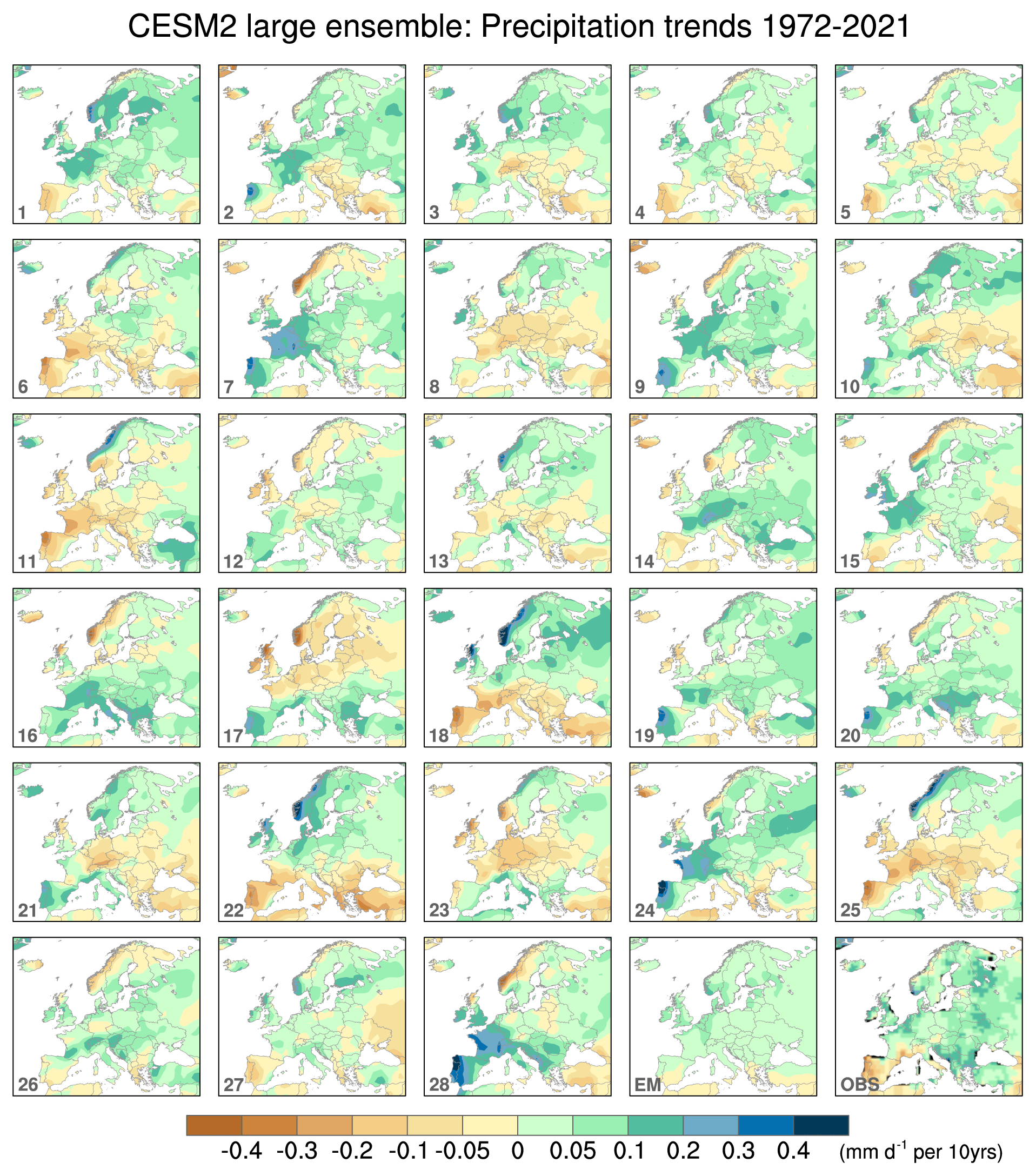
Figure 2 As in Fig. 1 but for precipitation (mm d⁻¹ per decade).

Like temperature, precipitation trends also vary considerably across ensemble members (Fig. 2). While the ensemble-mean trend shows modest increases in precipitation throughout Europe (except for the southernmost fringes), internal variability can evidently overwhelm the forced response in individual simulations. For example, some members show drying over large parts of the continent, while others depict enhanced wetting in the same regions (compare, for example, members 22 and 28, which show nearly opposite patterns). Observed precipitation trends are generally positive, except over Spain, Portugal, southern France, and other parts of the western Mediterranean (Fig. 2). The observed precipitation increases, while of the same sign as the model's forced response, are approximately twice as large in many areas. Again, the interpretation of the observed trends is ambiguous, since there are individual members that resemble observations (for example, member 1).

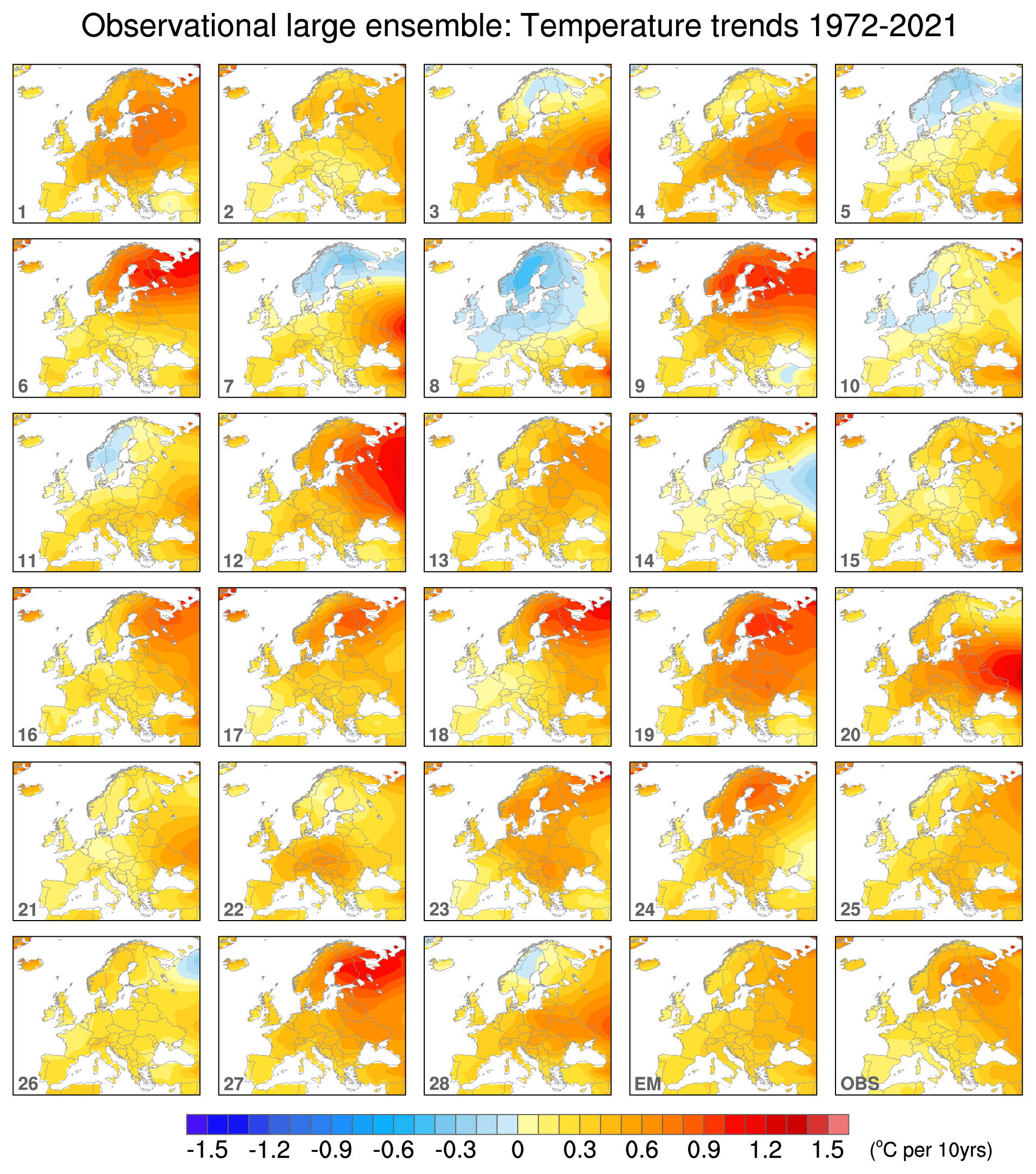
Figure 3 As in Fig. 1 but for the observational large ensemble of McKinnon and Deser (2018), with the ensemble mean from the 100-member CESM2 large ensemble. See text for details.

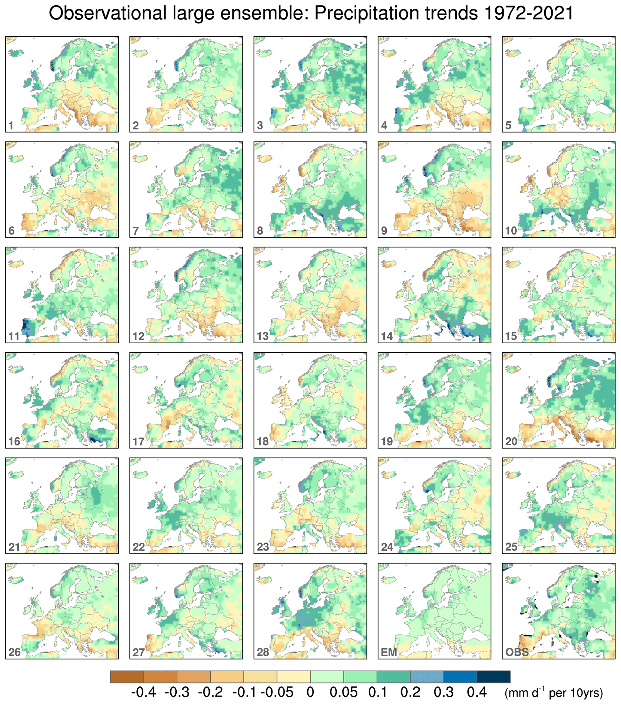
Figure 4 As in Fig. 2 but for the observational large ensemble of McKinnon and Deser (2018), with the ensemble mean from the 100-member CESM2 large ensemble. See text for details.

3.2 Past trends (1972–2021) in the OBS LE

The individual members of the OBS LE show a qualitatively similar diversity in the 50-year temperature trends as the CESM2 LE (Fig. 3). Like CESM2, some members show weak cooling in some areas, while others show widespread moderate or strong warming. This suggests that the resemblance between the observed trend and the model's forced response may be purely coincidental. Precipitation trends in the OBS LE also display large contrasts between members, similar to CESM2 (Fig. 4). For example, nearly opposite patterns are found between members 6 and 11 (or 8 and 9). Trend amplitudes also vary considerably across the OBS LE, with larger magnitudes in some members (for example, members 3 and 20) compared to others (e.g., members 21 and 13). While no single member of the 28 OBS LE samples shown matches the model's forced trend, member 21, with its relatively muted trends, comes close.

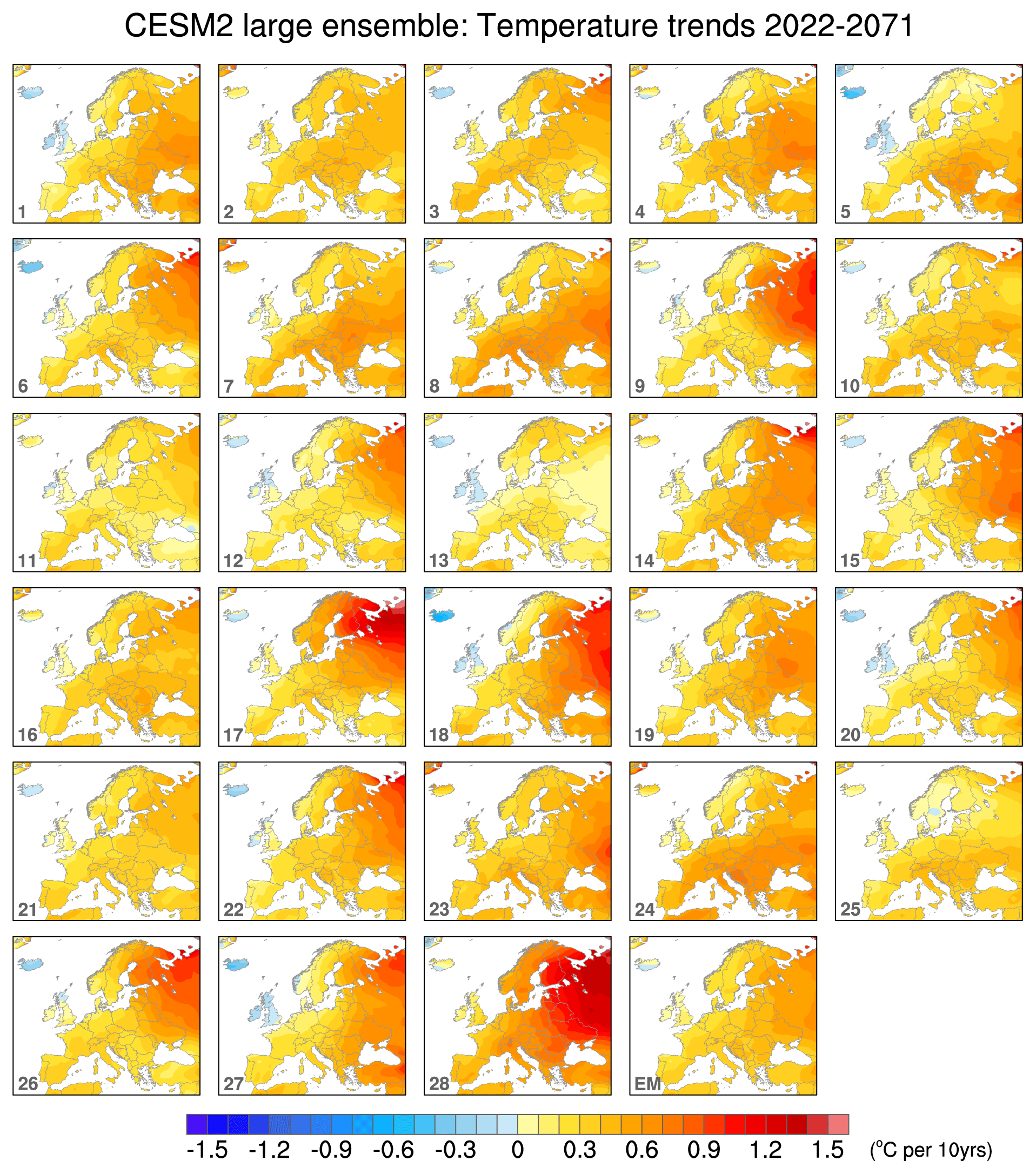
Figure 5 As in Fig. 1 but for the period 2022–2071.

3.3 Future trends (2022–2071) in the CESM2 LE

As expected, temperature trends projected for the next 50 years show larger amplitudes than those for the past 50 years in the CESM2 LE (Fig. 5). This is due to the fact that the forced (ensemble-mean) component of warming increases as greenhouse gas emissions accelerate. In most regions, the forced warming trend increases by approximately 0.2 ^∘C per decade in the future compared to the past. Notable exceptions are Iceland and the British Isles, which show less warming in the future due to a circulation-induced forced cooling trend (see Sect. 3.5). Despite a larger forced component, temperature trends projected for the next 50 years still show a wide range of amplitudes across individual members of the CESM2 LE. For example, member 13 is striking for its muted warming (generally <0.5 ^∘C per decade) across Europe (and absolute cooling over the UK and Iceland), while member 28 shows highly amplified warming, with values exceeding 1.3 ^∘C per decade over western Russia.

Figure 6 As in Fig. 2 but for the period 2022–2071.

Forced trends in precipitation are projected to amplify over the next 50 years, with greater wetting over northern Europe and drying over southern Europe and the Mediterranean (Fig. 6). In addition, the region with a forced drying trend is projected to expand northward into Spain, Italy, and the Balkans. While the forced pattern of future drying in the south and wetting in the north is generally evident in most of the simulations shown, there are notable differences in amplitude across the members. For example, member 28 shows precipitation trends in excess of 0.1 mm d⁻¹ per decade over most of northern Europe, while member 11 shows positive precipitation trends of less than half of this amount. Members 27 and 28 illustrate that the midsection of the European continent may become wetter or drier, depending on the unpredictable sequence of internal variability that unfolds. Thus, internal variability can still make a sizable contribution to the projected patterns and amplitudes of winter precipitation trends over the next 50 years.

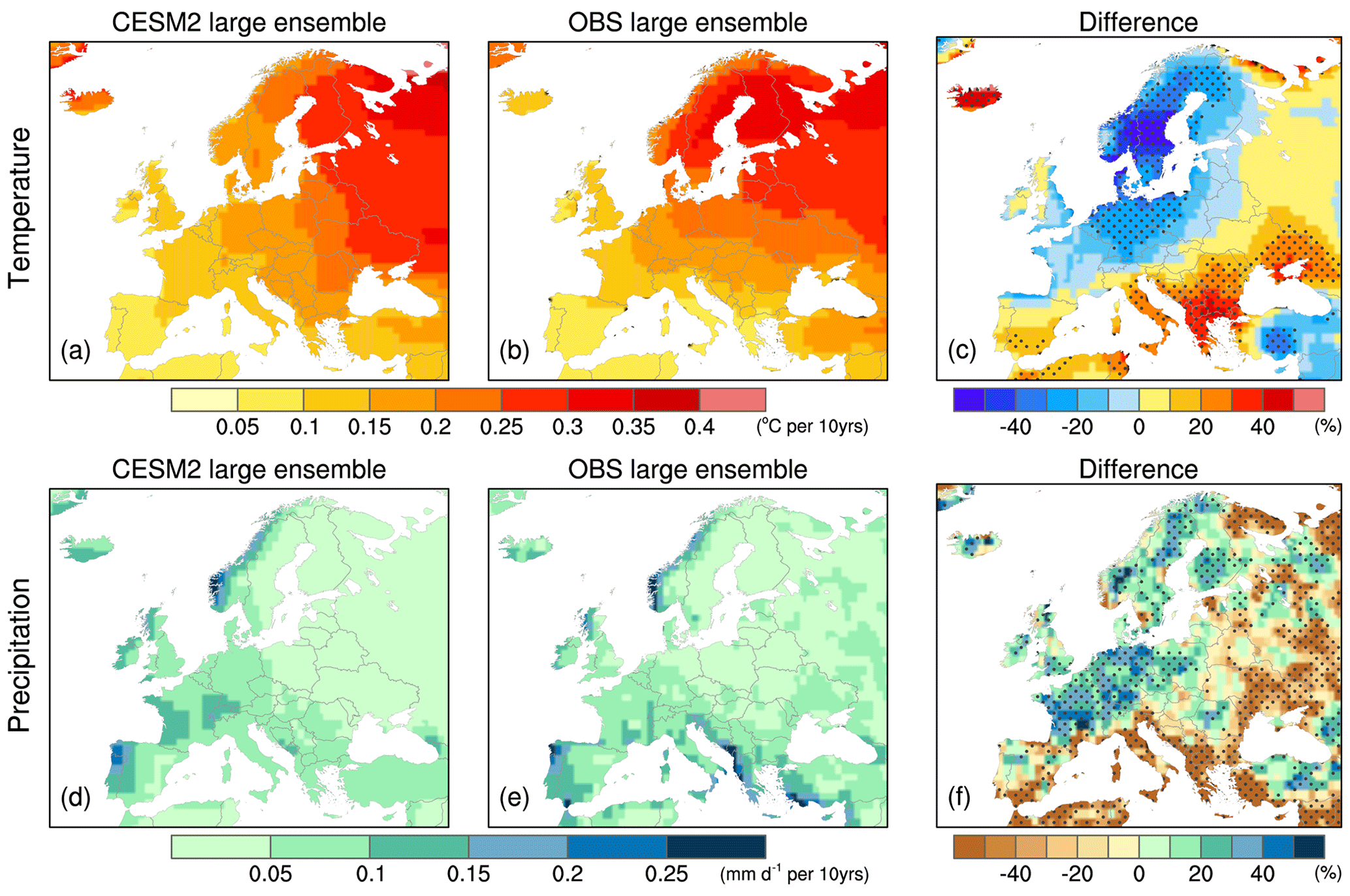
Figure 7 Standard deviation of 50-year trends (1972–2021) across 100 members of the CESM2 large ensemble (a, d) and 100 members of the observational large ensemble (b, e), and their difference (c, f) for winter air temperature (a–c; ^∘C per decade) and precipitation (d–f; mm d⁻¹ per decade). Stippling in panels (c) and (f) indicates that the differences are statistically significant at the 95 % confidence level according to an f test.

3.4 Signal-to-noise metrics and model evaluation

In the previous section, we conveyed a qualitative impression of the possible range of 50-year trends due to the superposition of internal variability and forced climate change in the CESM2 and OBS LEs. Here, we provide a more quantitative view, beginning with a comparison of the standard deviation (σ) of trends over the period 1972–2021 computed across the ensemble members of each LE. In the CESM2 LE, the ensemble σ of temperature trends increases from southwest to northeast, with minimum values (0.05–0.10 K per decade) over Spain and northern Africa and maximum values (0.30–0.35 0.5 ^∘C per decade) over northwestern Russia (Fig. 7a). A similar pattern is found in OBS LE, with some regional differences in amplitude (Fig. 7b). In particular, the ensemble σ values are significantly smaller (20 %–40 %) over Scandinavia, Germany, and Poland and significantly larger (20 %–40 %) in areas near the Mediterranean and Black seas in the OBS LE compared to the CESM2 LE (Fig. 7c). For precipitation trends, the two LEs show similar patterns of ensemble σ, with largest amplitudes generally along the west coasts (0.10–0.25 mm d⁻¹ per decade) and over southwestern Europe (values 0.05–0.10 mm d⁻¹ per decade; Fig. 7d and e). However, CESM2 LE significantly underestimates the OBS LE by more than 40 % along the Mediterranean and Black seas and parts of Russia and significantly overestimates the OBS LE by 20 %–40 % in many areas of western Europe (Fig. 7f).

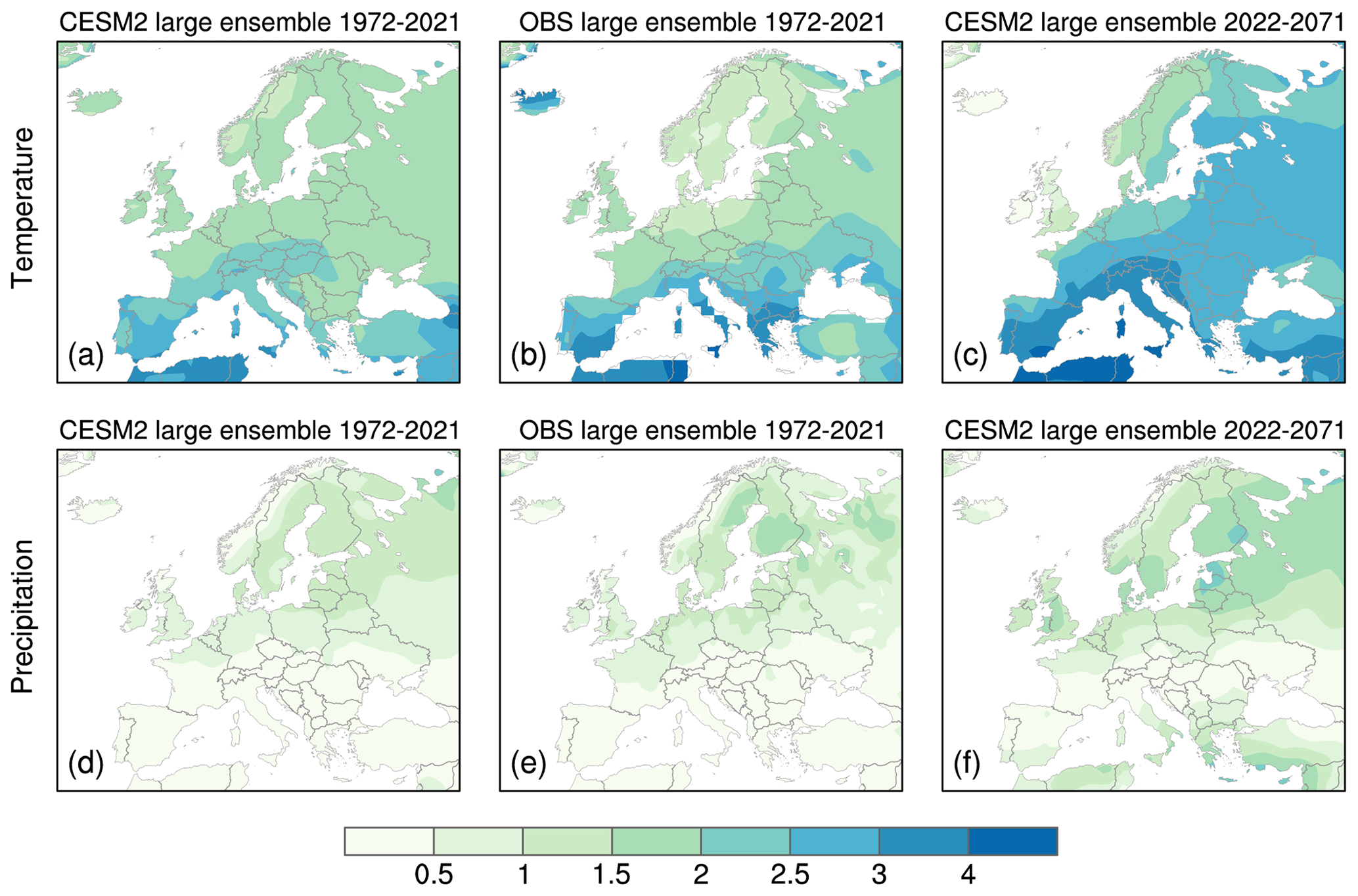
Figure 8 Signal-to-noise ratio of forced trends in winter (a–c) air temperature and (d–f) precipitation based on the 100-member CESM2 large ensemble during 1972–2021 (a, d), the observational large ensemble during 1972–2021 (b, e), and the CESM2 large ensemble during 2022–2071 (c, f). See text for details.

Next, we assess the relative magnitude of the forced and internal components of trends by computing a signal-to-noise ratio defined as the CESM2 ensemble-mean trend divided by the σ of trends across the 100 members of each LE. This signal-to-noise ratio provides a metric of the likelihood that the ensemble-mean (e.g., forced) trend might be overwhelmed by the internally generated trend in any given ensemble member (and, by extension, the real world). Assuming that the 100-member set of 50-year trends follows a normal distribution (not shown; see related results in Deser et al., 2012; Thompson et al., 2015; Deser et al., 2020a), a signal-to-noise ratio greater than one (two) indicates that the magnitude of the ensemble-mean (forced) trend is larger than (more than twice as large as) that of a typical (e.g., 1 standard deviation) internal trend, and a signal-to-noise ratio less than one indicates that the amplitude of a typical internal trend exceeds the magnitude of the forced trend. In the CESM2 LE, the signal-to-noise ratio of forced temperature trends over the past 50 years generally ranges from 1.5–2 over central and northern Europe and from 2–3 over southern Europe (Fig. 8a). Forced precipitation trends over the past 50 years exhibit much lower signal-to-noise ratios than temperature, with values generally <1 and nearly always <1.5 (Fig. 8d).

How much do model biases in the ensemble σ shown previously affect the signal-to-noise of the model's forced trends? We address this question by using the OBS LE σ values in place of the model's σ values in the signal-to-noise calculation (note that the signal in the two LEs is identical by construction). This substitution results in an enhancement of the signal-to-noise ratio of past forced temperature trends over southern Europe and a reduction in the signal-to-noise ratio over Scandinavia, Germany, and Poland, with a net increase from 38 % to 60 % in the area with values >2 (Fig. 8b). The impact of model biases in the ensemble trend σ is much less pronounced for precipitation than temperature, with signal-to-noise values in all locations remaining below 2 (Fig. 8e).

As expected, signal-to-noise values are higher for forced trends in the future than in the past. A total of 97 % of the area of the continent (excluding Iceland and Greenland) shows a signal-to-noise value >2 for forced temperature trends during 2022–2071 (Fig. 8c), compared with 38 % for trends during 1972–2021. Forced precipitation trends in the future remain uncertain, with only 2 % of the land area showing a signal-to-noise value >2 (Fig. 8f).

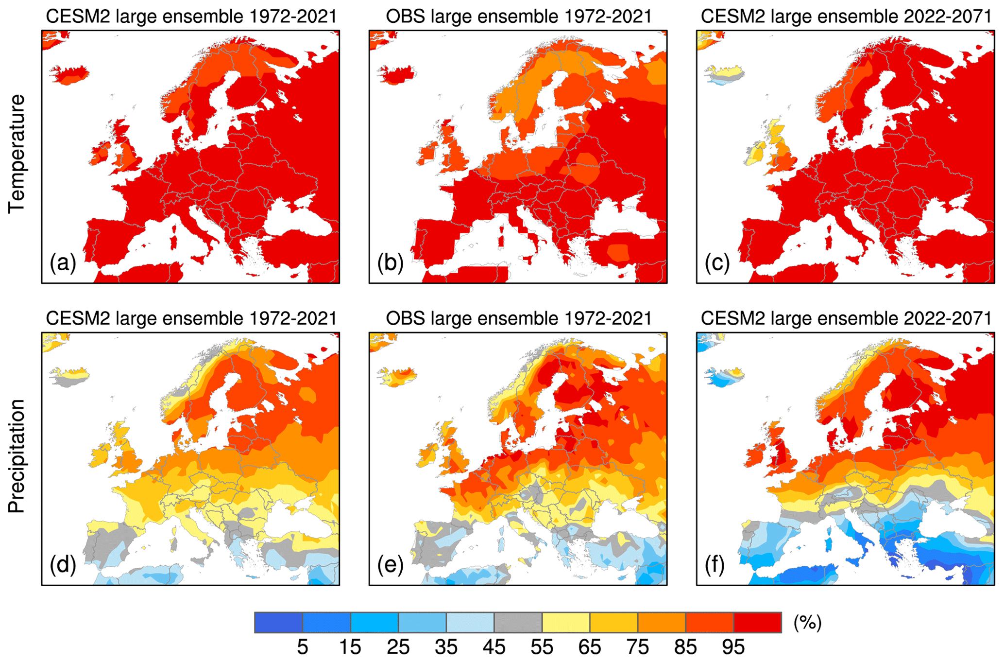
Figure 9 The percentage of ensemble members with a positive trend in winter (a–c) air temperature and (d–f) precipitation trends based on (a, d) the 100-member CESM2 large ensemble during 1972–2021, (b, e) the 100-member observational large ensemble during 1972–2021, and (c, f) the 100-member CESM2 large ensemble during 2022–2071.

Another way to view the relative impacts of internal variability and external forcing on trends is by computing the fraction of ensemble members at each location that shows a positive trend (e.g., warming or wetting). This metric conveys the likelihood of having a positive (or negative) trend in any single ensemble member, which is analogous to the single realization of the real world. At nearly all locations, more than 95 % of ensemble members in the CESM2 LE show warming in both the past and future periods, with slightly lower percentages (85 %–95 %) over western Scandinavia and parts of Great Britain (and <75 % over Ireland, Scotland, and Iceland in the future; Fig. 9a and c). Similar percentages are obtained when the internal component of past temperature trends in the OBS LE is used in place of the model's internal trends, with some reduction (75 %–95 %) over Scandinavia, northern Russia, Germany, and Poland (Fig. 9b).

The sign of the trend in any given ensemble member is more uncertain for precipitation than for temperature. The highest chances (>85 %) of a positive precipitation trend are found over the northernmost third of the continent, excluding Norway, both in the past and future (Fig. 9d and f). Similarly high chances of a negative precipitation trend (equivalent to <15 % of a positive trend) occur in areas near the Mediterranean Sea but only in the future. The central portion of the continent shows roughly equal chances of having a positive or negative trend, both in the past and future. The area with a >85 % chance of a positive precipitation trend in the past 50 years expands southward into northern France, Germany, and areas bordering the Baltic Sea when internal variability is derived from the OBS LE compared to the CESM2 LE (Fig. 9e).

Taken together, the results shown in Fig. 9 indicate that warming is virtually guaranteed at nearly all locations, both in the past 50 years and the next 50 years, according to the CESM2 LE. However, the sign of the precipitation trend (past and future) is robust only over the northern tier of the continent and only in the future over the Mediterranean region. The model results for past trends are found to be generally credible, as measured against the OBS LE, with some overestimation in north–central Europe.

3.5 Range of outcomes and the role of the atmospheric circulation

As the saying goes, “climate is what we expect; weather is what we get”. This adage is also applicable to climate change, where “human-induced climate change is what we expect; internal variability plus human-induced climate change is what we get” (Deser, 2020). Here, we illustrate “what we expect” and the range of “what we get” for past and future 50-year trends in the CESM2 LE, using the ensemble mean for what we expect and two contrasting ensemble members for the range of what we get. We select the contrasting members from the bottom and top 5th percentiles of the distribution of 100-member trends averaged over the European continent for each period separately. This selection criterion is somewhat arbitrary and neither necessarily captures the wide range of trend amplitudes that may occur at a single location or sub-region, nor does it portray the full range of spatial patterns that occur within the ensemble.

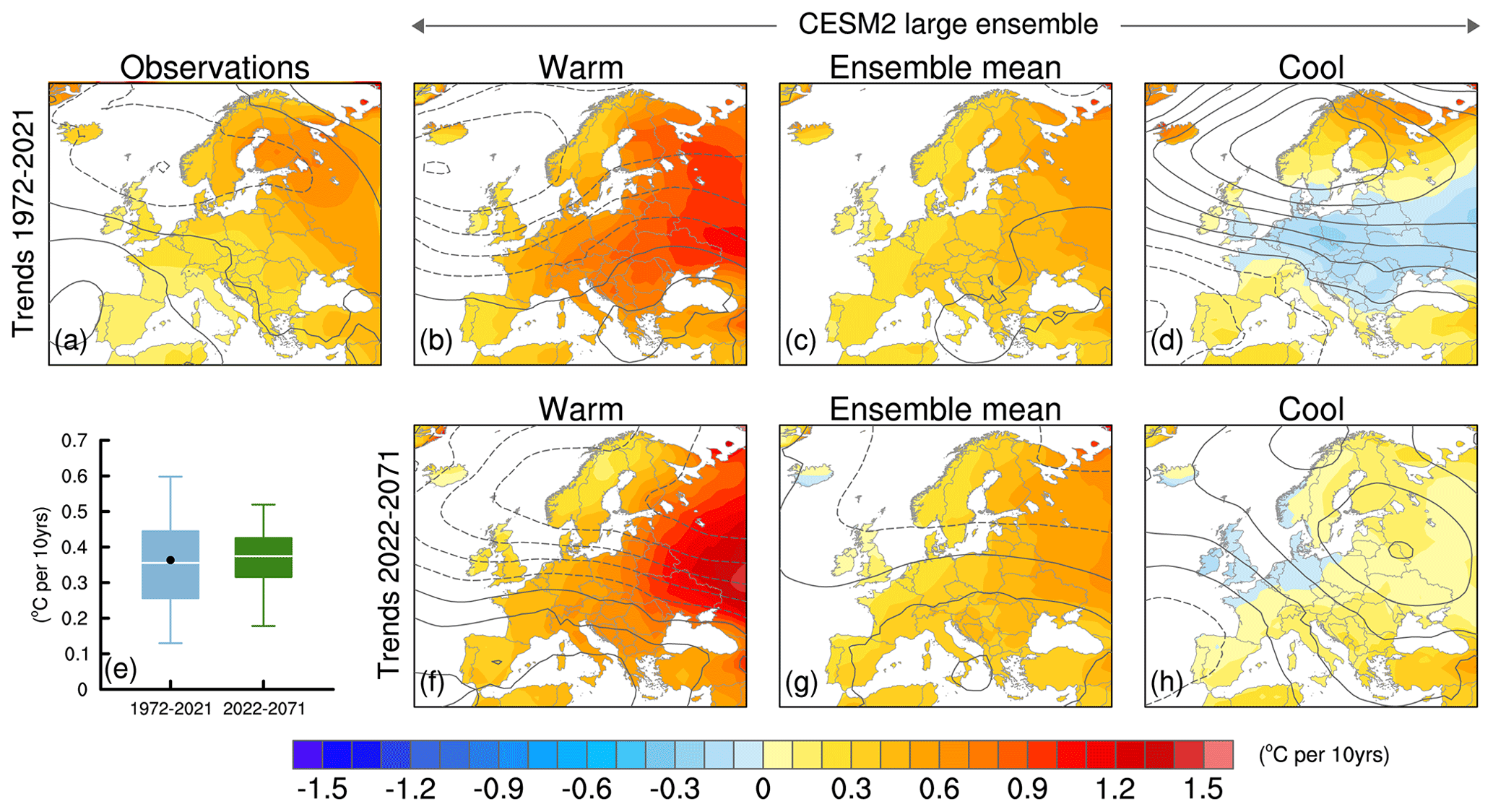
Figure 10 A range of outcomes. Trends in winter air temperature (color shading; ^∘C per decade) and sea level pressure (SLP) (contours; contour interval of 0.25 hPa per decade; negative values dashed) for the period (a–d) 1972–2021 and (e–h) 2022–2071. Panel (a) shows observed trends (1972–2021), and remaining panels show simulated trends from the 100-member CESM2 large ensemble. (c, g) Ensemble mean. (b, f) Warm end-member. (d, h) Cool end-member. See text for details. Note that panels (a) and (c) are identical to the OBS and EM panels in Fig. 1, respectively. (e) Distribution of European-averaged trends for 1972–2021 (blue) and 2022–2071 (green) from the CESM2 large ensemble (the box outlines 25th–75th percentile range, whiskers mark the 5th–95th percentile range, the horizontal white line denotes the median value, and the black circle marks the observed value).

There is a large range in temperature trend outcomes (what we get) for both the past 50 years and the next 50 years, as depicted by the warm and cool end-members (Fig. 10). For past trends, the warm end-member shows temperature increases of 0.9–1.1 ^∘C per decade over the eastern portion of the continent (Fig. 10b), while the cool end-member displays muted warming (<0.3 ^∘C per decade) and even slight cooling through the midsection of the continent (Fig. 10d). Clearly, the forced trend (what we expect), which depicts moderate warming (0.2–0.6 ^∘C per decade) across the continent does not tell the whole story (Fig. 10c). Analogous results are found for trends projected over the next 50 years; the warm member shows temperature increases of 1.0–1.5 ^∘C per decade over west–central Russia (Fig. 10f), while the cool member depicts <0.2 ^∘C per decade warming over most of the continent (Fig. 10h), which is in marked contrast to the forced trend which ranges from 0.3–0.6 ^∘C per decade (Fig. 10g). As discussed previously, the observed temperature trend map resembles the model's ensemble mean, but this could be by chance (Fig. 10a). In terms of European averages, the observed trend (0.36 ^∘C per decade) is nearly coincident with the median value of the model's trend distribution, which has a 5th–95th percentile range of 0.13–0.60 ^∘C per decade for past 50 years of trends (Fig. 10e). Curiously, the model's median trend value for Europe as a whole increases only slightly in the future compared to the past, while the 5th–95th and 25th–75th percentile ranges narrow (Fig. 10e). Further work is needed to understand why this is the case.

As mentioned in Sect. 1.4, previous work has shown that internal variability in the large-scale atmospheric circulation causes much of the member-to-member differences in temperature trends in model LEs. Here, we provide a qualitative indication of the circulation influence by superimposing SLP trends upon the maps in Fig. 10. In the case of past trends, the warm member shows a positive North Atlantic Oscillation (NAO)-like pattern (Hurrell et al., 2003), with negative SLP trends centered near Iceland and positive SLP trends centered over the Mediterranean (Fig. 10b). This SLP pattern is indicative of stronger westerly/southwesterly flow, which brings relatively warm maritime air over the continent. The cool member shows a largely opposite flow configuration (albeit with longitudinal shifts in the SLP centers of action), which advects relatively cold air from the east over the continent (Fig. 10d). In comparison, the forced response shows negligible atmospheric circulation change (Fig. 10c). Striking contrasts in circulation are also found for the future period, with a large positive NAO-like trend pattern in the warm member and a blocking continental high in the cool member (Fig. 10f and h). Future trends in SLP also contain a modest forced component indicative of enhanced westerlies over the continent (Fig. 10g).

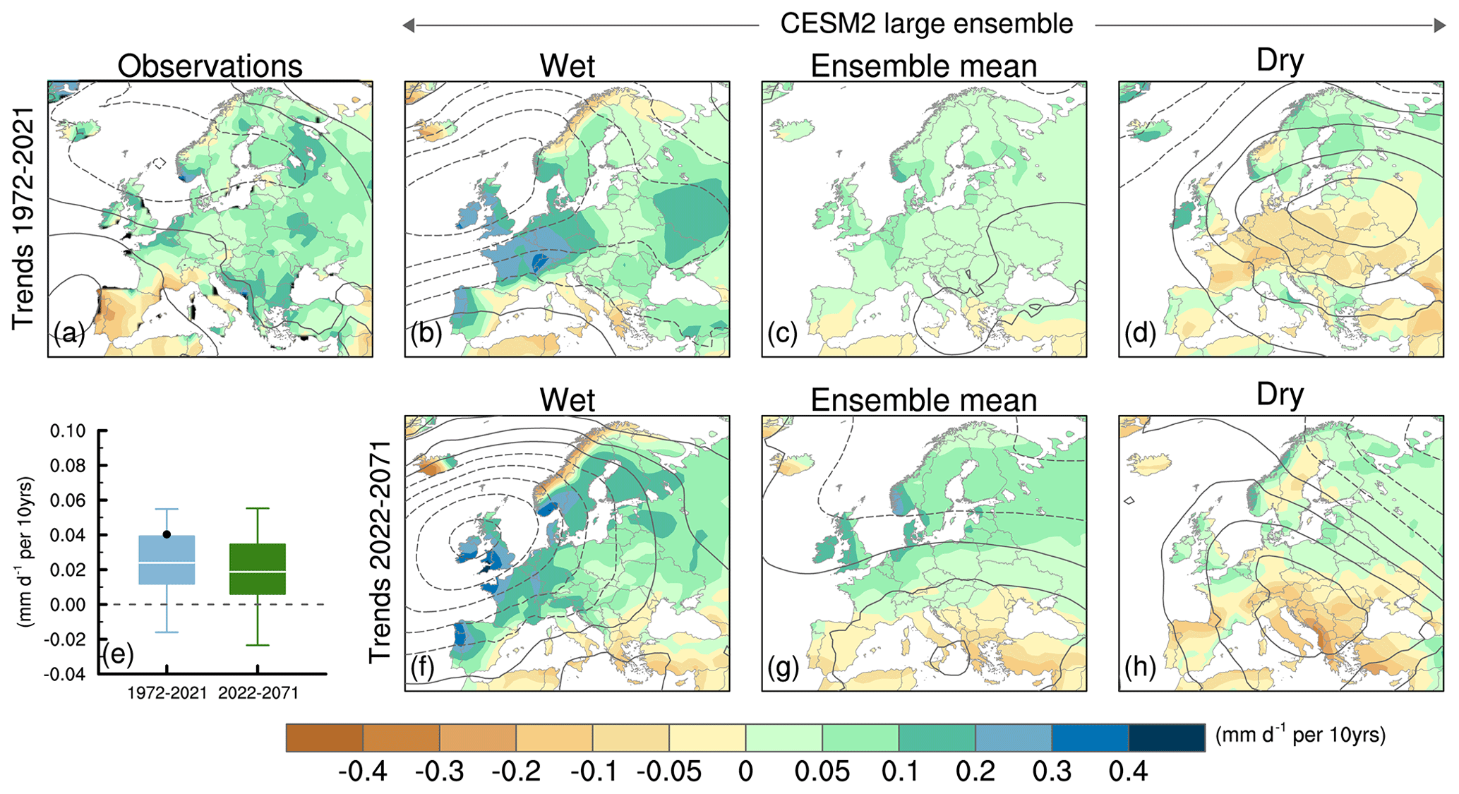
Figure 11 As in Fig. 10 but for precipitation (mm d⁻¹ per decade). Note that panels (a) and (c) are identical to the OBS and EM panels in Fig. 2, respectively.

The wet and dry end-members also show striking regional contrasts in both precipitation and circulation (Fig. 11). For example, for past trends, the wet member shows precipitation increases of 0.2–0.3 mm d⁻¹ per decade over France, southern Germany, Portugal, and the UK and precipitation declines over northern Norway and along the Mediterranean Sea (Fig. 11b). A nearly opposite pattern is found for the dry member (Fig. 11d). These contrasting precipitation trends can be understood in the context of the overlying atmospheric circulation changes, with wetter areas coinciding with anomalous westerly/southwesterly flow and drier areas located under blocking anticyclones. Analogous patterns are found for future trends, with pronounced increases in precipitation over western Europe associated with the low-pressure trend centered over the British Isles in the wet member (Fig. 11f) and generally reduced precipitation in the dry member associated with the blocking high centered over southern Europe (Fig. 11h).

3.6 Unmasking forced climate change in observations via dynamical adjustment

The empirical method of dynamical adjustment introduced in Sect. 1.4 can be used to estimate the circulation-induced component of observed temperature anomalies; this dynamically induced contribution can then be subtracted from the original anomaly to obtain the thermodynamically induced component as a residual. Since this method uses no information from climate models, it provides an independent estimate of the thermodynamic component of observed temperature trends, which can be compared with the forced response simulated by climate model LEs.

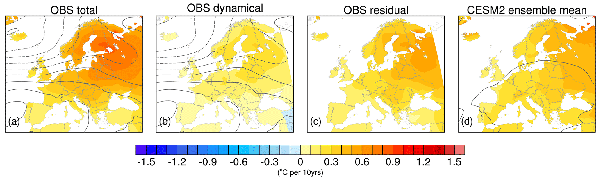
Figure 12 Decomposition of (a) observed winter air temperature trends (1962–2021; ^∘C per decade) into (b) dynamical and (c) residual thermodynamic contributions, using the dynamical adjustment procedure of Deser et al. (2018), based on constructed circulation analogues (see text for details). Contours in panel (a) show observed sea level pressure (SLP) trends (contour interval of 0.25 hPa per decade; negative values dashed), contours in panel (b) show the observed SLP trends estimated from the constructed circulation analogues, and contours in panel (c), based on the difference between panels (a) and (b), are near zero and not shown. Panel (d) shows the ensemble-mean temperature and SLP trends from the 100-member CESM2 large ensemble (note that only the zero contour shows up in panel d).

Figure 12 shows the decomposition of observed December–February (DJF) temperature trends into their dynamical and residual thermodynamic contributions. For this example, we have used the 60-year period 1962–2021, when observed SLP trends are more than twice as large as those during 1972–2021 on a per-decade basis (compare SLP contours in Figs. 10a and 12a). Observed SLP trends during the past 60 years show a pronounced positive NAO-like pattern, with maximum negative values of −1.25 hPa per decade near Iceland and maximum positive values of +0.75 hPa per decade west of Spain (Fig. 12a). Enhanced westerly/southwesterly flow associated with this pattern advects warm air, raising surface temperatures by 0.1–0.3 ^∘C per decade (with maximum warming over northern Europe), according to the dynamical adjustment algorithm (Fig. 12b). Removing this dynamically induced component from the total trend reveals the residual thermodynamic contribution to the observed warming trend (Fig. 12c). This observed thermodynamic trend is much closer in amplitude (and arguably pattern) to the model's forced response, as given by the CESM2 LE ensemble-mean trend (Fig. 12d), than is the total observed trend. Furthermore, the lack of an appreciable forced SLP trend in CESM2 indicates that the model's forced temperature trend is thermodynamically driven. The level of agreement between the observed thermodynamic temperature trend and the model's forced thermodynamic trend leads to the following two powerful conclusions: (1) The model's forced temperature trend is realistic, and (2) removing the circulation-induced component from the observed trends can effectively reveal the influence of anthropogenic forcing. Analogous results have been found for North America (Deser et al., 2016).

Figure 13 As in Fig. 12 but for precipitation (mm d⁻¹ per decade).

Precipitation is an inherently noisier field than temperature in both time and space, making it challenging to extract the forced signal via dynamical adjustment; indeed, only one previous study has attempted a dynamical adjustment of observed precipitation trends (Guo et al., 2019). Keeping in mind that the estimate of the circulation-induced component of precipitation trends may be less robust than for temperature, we present the results as a proof of concept. Observed precipitation trends during 1962–2021 are mainly driven by changes in atmospheric circulation, with a small thermodynamic residual component (Fig. 13). This residual component bears some resemblance to the forced response in CESM2, particularly in terms of amplitude (∼0.05 mm d⁻¹ per decade; Fig. 13d). Notable areas of agreement in the sign of the trends include drying over much of southern Europe and wetting over parts of northern Europe; central Europe shows less agreement in polarity. This is unsurprising, since this region was found to have a lower signal-to-noise ratio than other areas.

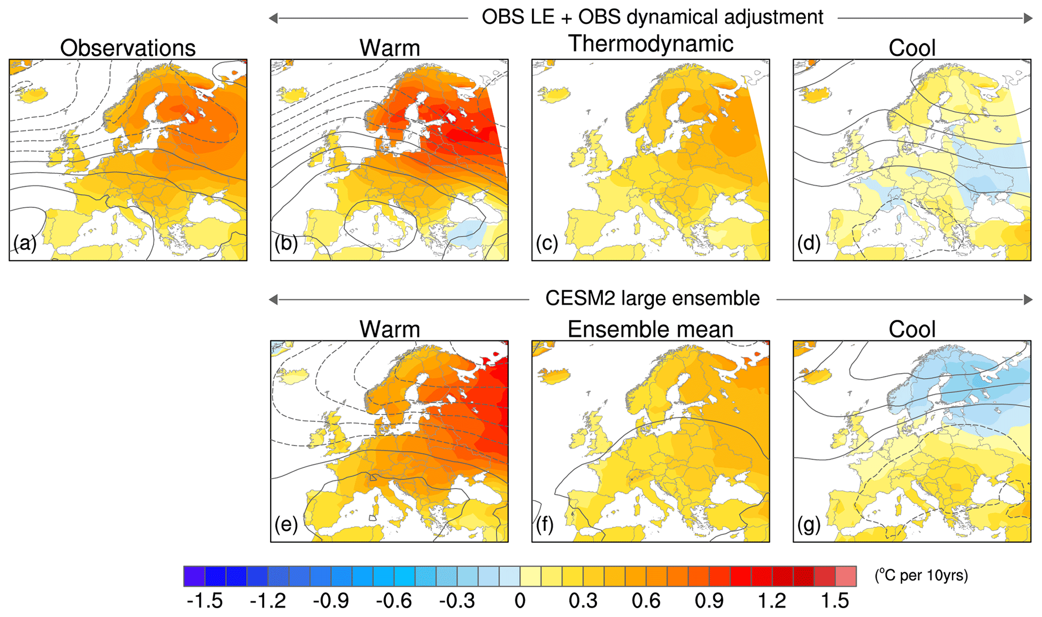
Figure 14 As in Fig. 10 but for the period 1962–2021. The top row (a–d) is based on the observational large ensemble combined with the residual thermodynamic component of observed trends. The bottom row (e–g) is based on the 100-member CESM2 large ensemble. See text for details.

3.7 Toward an observationally based range of outcomes

We conclude by bringing together the results of the observational LE and dynamical adjustment to produce a fully observationally based estimate of the range of the past 60 years of trends in temperature and precipitation. To the best of our knowledge, this is first time that these two approaches have been combined. Specifically, we add the internal component of trends from each member of the OBS LE to the thermodynamic residual trend (the estimate of the observed forced response) obtained from dynamical adjustment. As before, we select two contrasting ensemble members from the tails of the distribution based on Europe-wide averages to illustrate the range of trend outcomes. The warm end-member shows pronounced temperature increases over the northern two-thirds of the continent, with maximum values in excess of 0.9 ^∘C per decade, while the cool end-member warms less than 0.2 ^∘C per decade in most areas and even cools slightly over Ukraine and neighboring countries (Fig. 14b and d, respectively). These divergent temperature trends are associated with contrasting SLP trends, with a positive, NAO-like pattern in the warm member and a negative (and eastward-shifted) NAO pattern in the cool member (Fig. 14b and d). Qualitatively, this range of trend outcomes for both temperature and SLP is remarkably similar to that obtained directly from the CESM2 LE, with some regional differences in the location of cooling in the cool end-member (Fig. 14e and g). There is no guarantee that the patterns and amplitudes of trends sampled in our selected end-members will agree between the model and observationally based results, since there are many configurations that produce extremes in Europe-wide averages (not shown). That there is a strong qualitative resemblance between them is a testament to both the realism of the model's forced response and internal variability and the efficacy of the OBS LE and dynamical adjustment approaches.

Precipitation trends in the wet and dry end-members are also similar between the model and observationally based results (Fig. 15). The wet members show widespread increases in precipitation over southern and central Europe (maximum values of 0.2–0.4 mm d⁻¹ per decade) and drying over the northern UK and parts of Scandinavia (Fig. 15b and e). Largely opposite patterns prevail in the dry members (Fig. 15d and g). The contrasting precipitation trends in the wet and dry end-members are associated with opposite flow configurations, with regions of drying corresponding to high pressure, and vice versa.

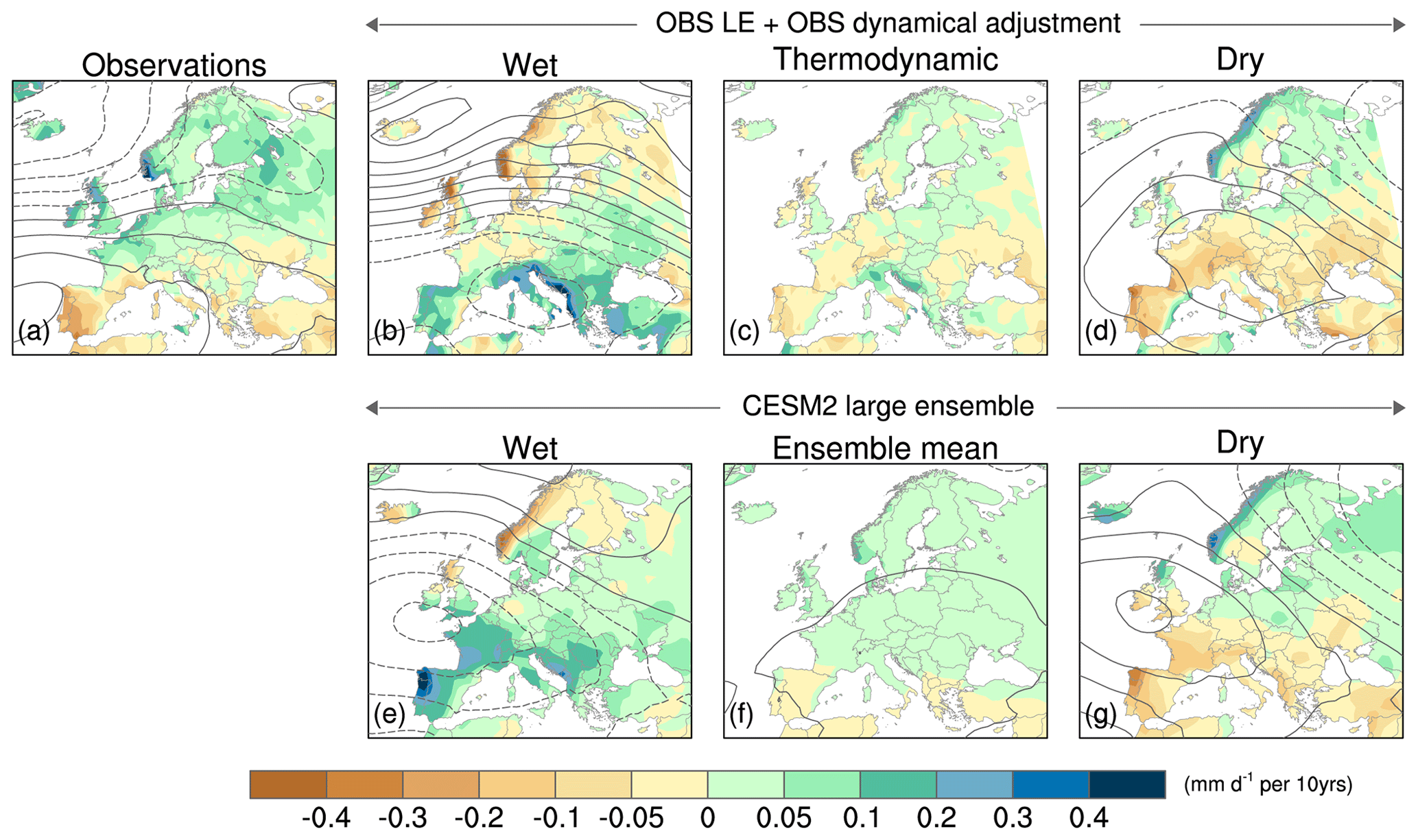
Figure 15 As in Fig. 14 but for precipitation (mm d⁻¹ per decade).

4 Summary and open questions

Disentangling the effects of internal variability and anthropogenic forcing on regional climate trends remains a long-standing issue in climate sciences. Recent advances in climate modeling and physical understanding have led to new insights about this topic and provided an improved source of information on the future risks of weather extremes associated with human-induced climate change. Here, we have highlighted new findings for European winter climate based on the following complementary tools: Earth system model large-ensemble simulations, an observationally based large ensemble, and an empirical approach for removing the influence of atmospheric circulation variability from observed temperature and precipitation data, which is termed dynamical adjustment.

The new 100-member CESM2 large ensemble shows that internal climate variability imparts considerable uncertainty to past and future 50-year trends in winter temperature and precipitation over Europe. Such uncertainty is irreducible due to the lack of predictability of the simulated internal variability on decadal timescales. A novel synthetic large ensemble constructed from the statistical characteristics of internal variability in the observational record exhibits quantitatively similar levels of uncertainty in the past 50 years of trends as the CESM2 LE, reinforcing the credibility of the model's internally generated trends. Additionally, the results of our dynamical adjustment procedure applied to observations shows good agreement between the observed thermodynamic residual trend component and the model's forced thermodynamic trend, further underscoring the realism of CESM2. Finally, we have combined internal variability in trends from an observational large ensemble with an observational estimate of the forced trend (the thermodynamic residual component obtained from dynamical adjustment) to show what the observed range of past trends in European temperature and precipitation could have been. Because it does not rely on climate model information, this observationally based range of trend outcomes provides a powerful test for the range of simulated trends in a model large ensemble. To the best of our knowledge, this is the first time that such a synthesis of the two purely observational methods has been undertaken.

Many outstanding questions remain regarding the relative influences of internal climate variability and anthropogenic forcing on regional climate change in models and the real world. Fortunately, promising new tools are being developed to help address these challenges. For example, innovative machine learning methods may be able to improve upon existing techniques for constructing observational large ensembles. Such methods have shown good results as statistical emulators of model-based LEs, but their application to the observational record remains to be pursued (Beusch et al., 2020). Similarly, neural network approaches to dynamical adjustment may offer increased skill compared to conventional methods (Davenport and Diffenbaugh, 2021) but have yet to be applied with the aim of separating forced and internal components of observed trends. Complementary physically based approaches such as linear inverse modeling and low-frequency pattern analysis, mentioned in Sect. 1.4, also offer promise for estimating the forced response in observations without reliance on climate models and should be pursued more widely.

We have relied on the fact that the CESM2 LE (like other models of its class; see Deser et al., 2020a, and references therein) simulates a negligible forced atmospheric circulation trend over the past 50–60 years to interpret our observed dynamical adjustment results (i.e., we have equated the observed dynamically induced trend with the internal component, and the observed thermodynamic residual trend with the forced component). If the model is erroneous in this regard, then our interpretation of our decomposition of observed trends into internal dynamical and forced thermodynamic components is flawed. Indeed, recent work suggests that climate models may be less predictable on seasonal-to-decadal timescales than the real world, particularly in terms of the large-scale extratropical atmospheric circulation (the so-called signal-to-noise paradox; e.g., Scaife et al., 2014; Eade et al., 2014; Scaife and Smith, 2018). But whether the results from such initial-value predictability studies carry over to the models' forced atmospheric circulation responses to anthropogenic emissions remains an open question. Finally, a recent study by Strommen et al. (2022) finds that the inclusion of stochastic parameterizations amplifies the simulated atmospheric circulation response to sea surface temperature and Arctic sea ice anomalies. Such stochastic parameterizations may represent unresolved air–sea coupling processes in coarse-resolution climate models such as CESM2. Emerging efforts to develop mesoscale–eddy-resolving global coupled climate models may provide more definitive answers to this elusive challenge in the near future.