An approach for projecting the timing of abrupt winter Arctic sea ice loss

Abrupt and irreversible winter Arctic sea ice loss may occur under anthropogenic warming due to the disappearance of a sea ice equilibrium at a threshold value of CO₂, commonly referred to as a tipping point. Previous work has been unable to conclusively identify whether a tipping point in winter Arctic sea ice exists because fully coupled climate models are too computationally expensive to run to equilibrium for many CO₂ values. Here, we explore the deviation of sea ice from its equilibrium state under realistic rates of CO₂ increase to demonstrate for the first time how a few time-dependent CO₂ experiments can be used to predict the existence and timing of sea ice tipping points without running the model to steady state. This study highlights the inefficacy of using a single experiment with slow-changing CO₂ to discover changes in the sea ice steady state and provides a novel alternate method that can be developed for the identification of tipping points in realistic climate models.

1 Introduction

The Arctic is warming at a rate at least twice as fast as the global mean with profound consequences for its sea ice cover. Sea ice is already exhibiting rapid retreat with warming, especially in the summertime (Comiso and Parkinson, 2004; Nghiem et al., 2007; Stroeve et al., 2008; Notz and Stroeve, 2016; Stroeve and Notz, 2018), shortening the time that socioeconomic and ecological systems have to adapt. These concerns have motivated a large body of work dedicated to both observing present-day sea ice loss (Kwok and Untersteiner, 2011; Stroeve et al., 2012; Lindsay and Schweiger, 2015; Lavergne et al., 2019) and modeling sea ice to understand whether its projected loss is modulated by a threshold-like or “tipping point” behavior. Abrupt loss of Arctic sea ice could be driven by local positive feedback mechanisms (Curry et al., 1995; Abbot and Tziperman, 2008; Abbot et al., 2009; Kay et al., 2012; Leibowicz et al., 2012; Burt et al., 2016; Feldl et al., 2020; Hankel and Tziperman, 2021), remote feedback mechanisms that increase heat flux from the midlatitudes (Holland et al., 2006; Park et al., 2015), or by the natural threshold corresponding to the seawater freezing point (Bathiany et al., 2016). If such an abrupt loss is caused by irreversible processes (typically, strong positive feedback mechanisms as opposed to the reversible mechanism of a freezing point threshold of Bathiany et al., 2016), it is referred to here as a tipping point. A tipping point in the sense used here is a change in the number or stability of steady-state solutions (Ghil and Childress, 1987; Strogatz, 1994) as a function of CO₂ and is also known as a bifurcation. We note that some of the climate literature uses the term tipping point in a more general sense of a relatively rapid change (e.g., Lenton, 2012). While most studies have concluded that there is no tipping point during the transition from perennial to seasonal ice cover (i.e., during the loss of summer sea ice), the existence of a tipping point during the loss of winter sea ice (transition to year-round ice-free conditions) continues to be debated in the literature (Eisenman, 2007, 2012; Eisenman and Wettlaufer, 2009; Notz, 2009). Wagner and Eisenman (2015) showed that a winter tipping point disappeared from a simple model of sea ice with no active atmosphere when a longitudinal dimension was added. On the other hand, other literature (e.g., Abbot and Tziperman, 2008; Hankel and Tziperman, 2021) has demonstrated the importance of atmospheric feedbacks, not included in the model of Wagner and Eisenman (2015), in inducing winter sea ice tipping point. Furthermore, three out of seven fully complex global climate models (GCMs) that lost their winter sea ice completely in the CMIP5 extended RCP8.5 scenario showed a very abrupt change in winter Arctic sea ice resembling a tipping point (Hezel et al., 2014; Hankel and Tziperman, 2021). However, given the projected rapid changes to CO₂ in the coming centuries and the slower response of the climate system, we do not expect future sea ice to be fully equilibrated to the CO₂ forcing at a given time, making the standard steady-state tipping point analysis challenging. Thus, our first goal is to understand abrupt winter Arctic sea ice changes – which may or may not be due to tipping points – under rapidly changing CO₂ forcing, where sea ice is not at equilibrium.

Tipping points imply a bistability (meaning that sea ice can take on different values for the same CO₂ concentration), and hysteresis – an irreversible loss of sea ice even if CO₂ is later reduced. Bistability (and therefore tipping points) can be tested for by running model simulations to steady state at many different CO₂ values, which is computationally inefficient in expensive, state-of-the-art GCMs. GCM studies, therefore, tend to use a single experiment with very gradual CO₂ increases and decreases (Li et al., 2013) or even a faster CO₂ change (Ridley et al., 2012; Armour et al., 2011) and look for hysteresis in sea ice that would imply the existence of a tipping point. These studies implicitly assume that such a run should approximate the behavior of the steady state at different CO₂ concentrations. However, Li et al. (2013) further integrated two apparently bistable points and found that they equilibrated to the same value of winter sea ice: there was no “true” bistability at these two CO₂ concentrations, the sea ice was simply out of equilibrium with the CO₂ forcing. This calls into question the current use of time-changing CO₂ runs to study the bifurcation structure of sea ice.

In light of the difficulties in using climate model runs with time-changing CO₂ (hereafter “transient runs”), the first goal of this work is to understand the relationship between these transient runs and the steady-state value of sea ice in systems with and without bifurcations (since the existence of a bifurcation in winter sea ice remains unknown), and the second goal is to develop a new efficient method for the identification of tipping points from transient runs. Theoretical work in dynamical systems (Haberman, 1979; Mandel and Erneux, 1987; Baer et al., 1989; Tredicce et al., 2004) and studies related to bistability in the Atlantic Meridional Overturning Circulation (AMOC; Kim et al., 2021; An et al., 2021) have examined systems with tipping points when the forcing parameter (CO₂ in our case) changes in time at a finite rate. They found that as the forcing parameter passes the bifurcation point, the system continues to follow the old equilibrium solution for some time before it rapidly transitions to the new one. Specifically, Kim et al. (2021) and An et al. (2021) find that the width of the hysteresis loop of AMOC is altered by the rate of forcing changes – this phenomenon is referred to as “rate-dependent hysteresis”. This rate dependence occurs in their case in a system that also has bistability and hysteresis in the equilibrium state. This type of analysis has, to our knowledge, not yet been applied in the context of winter sea ice loss under time-changing CO₂ concentrations nor compared in systems with and without a bifurcation (that is, with and without an equilibrium hysteresis).

In order to analyze how the hysteresis of sea ice under time-changing forcing relates to the steady-state behavior of sea ice, we run a simple physics-based model of sea ice (Eisenman, 2007), configured in three different scenarios: with a large CO₂ range of bistability, a small range of bistability, and no bistability in the equilibrium. These three scenarios span the range of possible behaviors of winter sea ice in state-of-the-art climate models. Each case is run with different rates of CO₂ increase (ramping rates). We use results from this model and from an even simpler standard 1D dynamical system to demonstrate that the convergence of the transient behavior (under time-changing forcing) to the equilibrium behavior is very slow as a function of the ramping rate of CO₂. In other words, even climate model runs with very slow-changing CO₂ forcing may simulate sea ice that is considerably out of equilibrium near the period of abrupt sea ice loss. Finally, we propose a novel approach for uncovering the underlying equilibrium behavior – and thus the existence and location of tipping points – in comprehensive models where it is computationally infeasible to simulate steady-state conditions for many CO₂ values. Such a method is important given the model-dependent nature of winter sea ice tipping points discussed above; uncovering the existence of sea ice tipping points in GCMs, which are the most realistic representation of Arctic-wide sea ice behavior that we have, is the next step toward understanding whether such tipping points exist in the real climate system. Our goal has some parallels to that of Gregory et al. (2004), who used un-equilibrated GCM runs to deduce the equilibrium climate sensitivity when fully equilibrated runs were computationally infeasible.

As mentioned above, some GCMs exhibit an abrupt change in winter sea ice that may be a tipping point, and others do not (Hezel et al., 2014; Hankel and Tziperman, 2021). The reasons likely involve numerous differences in parameters and parameterizations. It is not obvious how to modify parameters in a single GCM to display all of these different behaviors. Therefore, we choose to use an idealized model of sea ice where we can directly produce different bifurcation behaviors to address our second goal and answer the question: is it possible to identify the CO₂ at which tipping points occur without running the model to a steady state for many CO₂ values? Answering such a question in a simple model is an obvious prerequisite to tackling the problem of identifying climate bistability in noisy, high-dimensional GCMs. In order to perform this analysis for each of the three scenarios mentioned above, we modify the strength of the albedo feedback via the choice of surface albedo parameters. The albedo values used here to generate the three scenarios are not meant to reflect realistic albedo values but rather allow us to represent in a single model the range of sea ice equilibria behaviors that may exist in different GCMs. We, therefore, follow in the footsteps of previous studies (e.g., Eisenman, 2007) that have also changed parameters outside of their physically relevant regime in order to understand summer sea ice bifurcation behavior; here we follow the same approach to understand when a winter sea ice bifurcation can be detected without running an expensive climate model to steady state.

2 Methods

2.1 Sea ice model

The sea ice model used follows Eisenman (2007) almost exactly, and its key features are depicted schematically in Fig. 1. The model contains four state variables: sea ice effective thickness (V, which is volume divided by the area of the model grid box), sea ice area (A), sea ice surface temperature (T_i), and mixed-layer temperature (T_ml) for a single box representing the entire Arctic. Subsequent versions of this sea ice model have been used in Eisenman and Wettlaufer (2009), Eisenman (2012), and Wagner and Eisenman (2015). Those versions are derived from the model used here, making a few further modest simplifications (using a hyperbolic tangent function for surface albedo, assuming the ice surface temperature is in a steady state, combining all prognostic variables into one, i.e., enthalpy) that do not affect the qualitative behavior of the model (i.e., the nature of summer and winter sea ice bifurcations). We choose to implement the earlier model because it explicitly represents the key physical variables of ice volume, area, ocean temperature, and ice temperature as prognostic variables – as opposed to combining them all into a single enthalpy – and thus provides more transparency and interpretability. We, therefore, do not expect our results to change if we use any of the later model versions.

Figure 1 Schematic showing some of the key features of the Eisenman (2007) model. Its four prognostic variables are ice volume, ice area, ice surface temperature, and ocean mixed-layer temperature. The full model equations can be found in the Supplement.

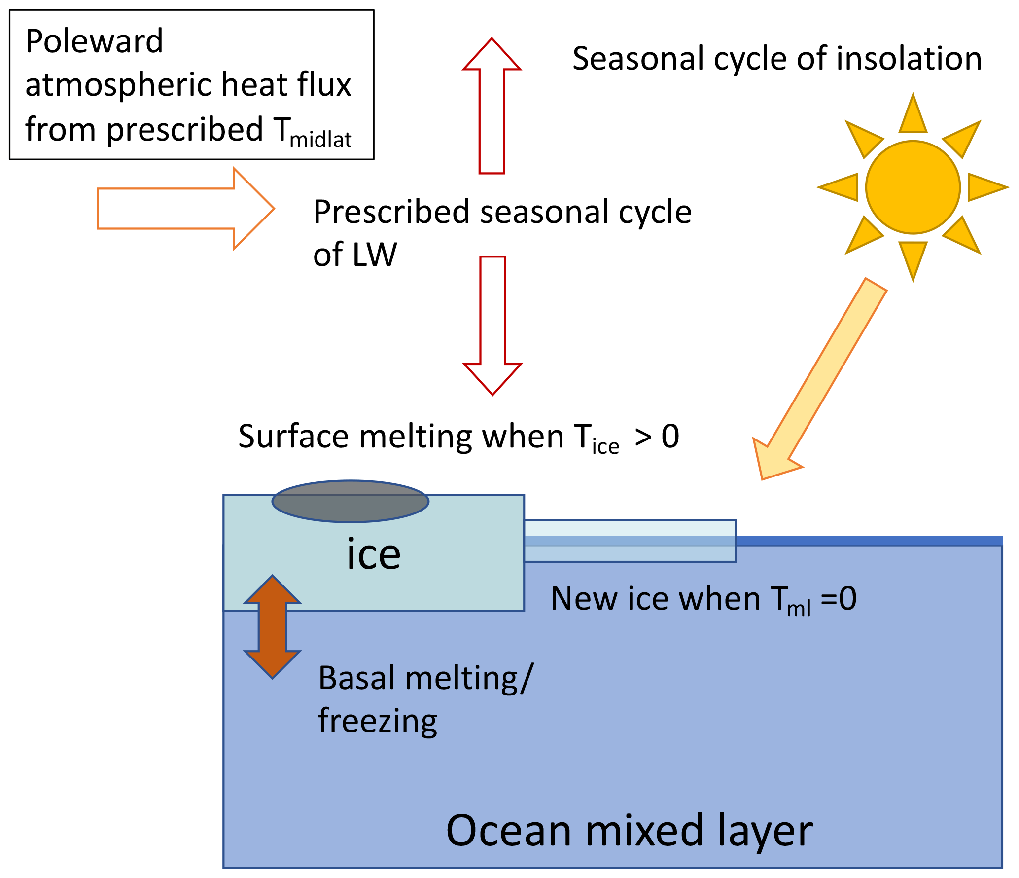
In the model, the atmosphere is assumed to be in radiative equilibrium with the surface, and the model is forced with a seasonal cycle of insolation; of poleward atmospheric heat transport from the midlatitudes; and of local optical thickness of the atmosphere, which represents cloudiness. Sea ice growth and loss are primarily determined by the heat budget at the bottom of the ice and are therefore set by the balance between ocean–ice heat exchanges and heat loss through the ice to the atmosphere. When conditions for surface melting are met (when the ice surface temperature is zero and net fluxes on the ice are positive), all surface heating goes into melting ice and the surface albedo of the ice is set to the melt pond albedo. The ocean temperature is affected by shortwave and longwave fluxes in the fraction of the box that is ice-free and by ice–ocean heat exchanges. When the ocean temperature reaches zero, all additional cooling goes into ice production, while the ocean temperature remains constant. The full equations of the sea ice model can be found in the original paper (Eisenman, 2007) and in the Supplement; here, we highlight a few minor ways in which our implementation differs. First, for simplicity, we do not model leads, which in the original model were represented by capping the ice fraction at 0.95 rather than 1. Second, we use an approximation to the seasonal cycle of insolation (Hartmann, 2015) using a latitude of 75^∘ N. The atmospheric albedo is set to 0.425 to produce the same magnitude of the seasonal cycle as in the original model of Eisenman (2007).

2.2 Setup of simulations

In our transient-forcing scenarios (described below), we vary CO₂ in time which affects the prescribed near-surface atmospheric midlatitude temperature (T_midlat) and the atmospheric optical depth (N; see the Supplement). Specifically, we increase the annual mean of T_midlat by 3 ^∘C per CO₂ doubling and N by a ΔN that corresponds to 3.7 W m⁻² per doubling. All model parameters are as in Eisenman (2007) except as mentioned below.

We configure the model in three different scenarios that yield a wide CO₂ range of bistability in winter sea ice (Scenario 1), a small range of bistability in winter sea ice (Scenario 2), and no bistability in winter sea ice (Scenario 3). We do so by modifying the strength of the ice–albedo feedback by changing the albedos of bare ice (α_i), melt ponds (α_mp), and ocean (α_o), as listed in Table S1 in the Supplement.

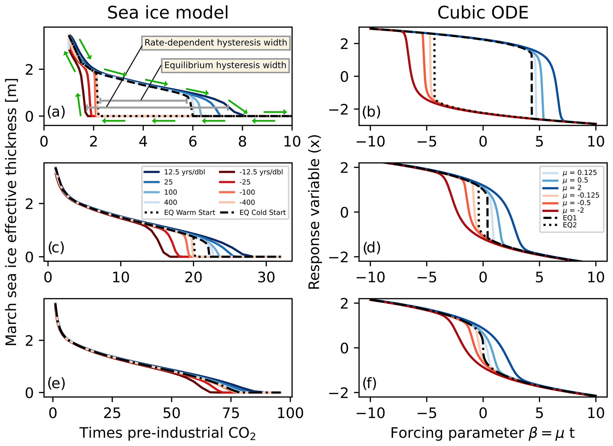
Figure 2 Hysteresis runs (time-changing forcing) and equilibrium runs (fixed forcing) for average March sea ice effective thickness (sea ice volume divided by area of the grid cell; panels a, c, and d) and the simple ODE from Eq. 1 (b, d, and f). The first row corresponds to Scenario 1 (wide bistability), the second row to Scenario 2 (narrow bistability), and the third to Scenario 3 (no bistability). Blue lines indicate simulations with increasing forcing (CO₂ or β), while red lines indicate simulations with decreasing forcing. Dashed and dotted black lines indicate the steady-state values of sea ice or the ODE variable x. These two black lines are different when the two initial conditions evolve to two different steady states. The legends indicate the different ramping rates (represented by darker colors for faster rates), which are in units of years per CO₂ doubling in the case of the sea ice model. The green arrows demonstrate the direction of evolving sea ice effective thickness during the hysteresis experiments.

In each of the three scenarios, we tune the model (by adjusting the mean and amplitude of the atmospheric optical depth) to roughly match the observed seasonal cycle of ice thickness under pre-industrial CO₂ (∼ 2.5–3.7 m, Eisenman, 2007). We then run each scenario with multiple CO₂ ramping rates (expressed in “years per doubling”) with an initial stabilization period (fixed pre-industrial CO₂), a period of exponentially increasing CO₂ concentration (which corresponds to linearly increasing radiative forcing), another period of stabilization at the maximum CO₂, a period of decreasing CO₂, and a final period of stabilization at the minimum CO₂ value (see Fig. S2 in the Supplement). Scenarios 2 and 3 are ramped to higher final CO₂ values than Scenario 1 so that they lose all their sea ice. We also directly calculate the steady-state behavior of the sea ice (as done in the original study) by running many simulations with fixed CO₂ values until the seasonal cycle of all the variables stabilizes. Because we expect multiple equilibria (which could be ice-free, seasonal ice, or perennial ice) at some CO₂ values in Scenarios 1 and 2, we run these steady-state simulations starting with both a cold (ice-covered) and a warm (ice-free) initial condition in order to find these different steady states. In the ice-free initial condition runs, the ice–albedo feedback will still play an important role if the temperature cools sufficiently for ice to develop. At CO₂ values for which the sea ice is bistable, the ice-free initial condition evolves to a perennially ice-free steady state, and the ice-covered initial condition evolves to a seasonally ice-covered steady state (seen by the dotted and dashed lines, respectively, in Fig. 2a and c).

2.3 Cubic ODE

The main points we are trying to make about the transient versus equilibrium behavior of winter sea ice near a tipping point are not unique to the problem of winter sea ice, and in order to demonstrate this, we use the simplest mathematical model that can display tipping points, following other studies that have also used such simple dynamical systems (Ditlevsen and Johnsen, 2010; Bathiany et al., 2018; Ritchie et al., 2021; Boers, 2021). The cubic ODE used, while much simpler than the sea ice model above, has some of the key characteristics of the sea ice system (it is a non-autonomous system due to the time-dependent forcing and has saddle–node bifurcations), which allows for direct comparison between the two models. The ODE equation,

$$\begin{array}{}\text{(1)}& {\displaystyle \frac{\mathrm{d}x}{\mathrm{d}t}}=-x^{\mathrm{3}}+\mathit{\delta }x+\mathit{\beta }\left(t\right),\mathit{\beta }\left(t\right)={\mathit{\beta }}_{\mathrm{0}}+\mathit{\mu }t,\end{array}$$

contains a time-changing forcing parameter, β(t) mimicking the effects of CO₂ in the sea ice model. We consider this differential equation in three scenarios, paralleling those used with the sea ice model: in Scenario 1, δ=5 leading to a wide region of bistability; in Scenario 2, δ=1 leading to a narrow region of bistability; and finally, in Scenario 3, δ=0 leading to a mono-stable system. The different values of δ, therefore, produce the same three scenarios that were achieved in the sea ice model by modifying the strength of the ice–albedo feedback. We mimic the hysteresis experiments of the sea ice model with a sequence of ramping up and ramping down (using different ramping rates, μ) with values of β ranging from −10 to 10 to sweep the parameter space that contains the bifurcations. We calculate the steady states with fixed values of β (μ=0), starting with both a positive and a negative initial condition of x to yield two stable solutions when these exist.

We want to calculate the upper and lower CO₂ values of the hysteresis region in runs with time-changing (i.e., transient) CO₂ forcing. We do so by calculating the CO₂ value at which the March sea ice area drops below a critical threshold (50 % ice coverage; results are insensitive to the specific value used) during increasing and decreasing CO₂ integrations: we denote these CO₂ values ${\mathrm{CO}}_{\mathrm{2}}^{\mathrm{i}}$ and ${\mathrm{CO}}_{\mathrm{2}}^{\mathrm{d}}$, respectively (see Fig. S9). The difference between ${\mathrm{CO}}_{\mathrm{2}}^{\mathrm{i}}$ and ${\mathrm{CO}}_{\mathrm{2}}^{\mathrm{d}}$ is referred to below as the “hysteresis width” of the rate-dependent hysteresis whether an equilibrium hysteresis exists or not; this width approaches the width of bistability at very slow ramping rates.

2.4 A new method for predicting the CO₂ of the sea ice tipping point

One of our main goals (see the Introduction) is to efficiently estimate the equilibrium behavior of sea ice, including the location of tipping points, without running the model to a steady state for many CO₂ values. This would show that such estimation could be calculated for GCMs where tipping points cannot be detected using steady-state runs due to their computational cost. In order to estimate the values of ${\mathrm{CO}}_{\mathrm{2}}^{\mathrm{i}}$ and ${\mathrm{CO}}_{\mathrm{2}}^{\mathrm{d}}$ that would have occurred for an infinitely slow ramping rate (in other words, the range of CO₂ for which there is bistability) using only the transient runs, we fit a polynomial of the form $f\left(x\right)=m{x}^c+b$ to ${\mathrm{CO}}_{\mathrm{2}}^{\mathrm{i}}$ and ${\mathrm{CO}}_{\mathrm{2}}^{\mathrm{d}}$ as functions of the ramping rate x. Because c is negative, the fitted parameter b represents the prediction of ${\mathrm{CO}}_{\mathrm{2}}^{\mathrm{i}}$ and ${\mathrm{CO}}_{\mathrm{2}}^{\mathrm{d}}$ at infinitely slow ramping rates, i.e., in the steady state. We also calculate the uncertainty in the fitted parameter b by block bootstrapping to account for autocorrelation; see the Supplement. Other fits to ${\mathrm{CO}}_{\mathrm{2}}^{\mathrm{i}}$ and ${\mathrm{CO}}_{\mathrm{2}}^{\mathrm{d}}$ as a function of ramping rates, such as an exponential function $f\left(x\right)=a+b\text{exp}(-cx)$, could in principle be used, although we found that fit to be less good in our case.

3 Results

In the following three subsections, we discuss the behavior of the sea ice model and the cubic ODE under time-changing forcing, the relationship of the transient and equilibrium behaviors, and a method that we propose for inferring the existence and location of tipping points from the transient behavior. Equilibrium hysteresis refers here to the path-dependent solution of a variable due to bistability and a bifurcation in the steady state (in other words, the loop traced by the steady-state solutions). The term rate-dependent hysteresis (An et al., 2021; Manoli et al., 2020) describes hysteresis loops that appear in time-changing forcing runs (rather than in the steady state) and that depend on the rate of forcing change. In our analysis rate-dependent hysteresis applies to both systems with and without equilibrium hysteresis: it refers to any differences in the results for increasing vs. decreasing CO₂ simulations of sea ice that are altered by the rate of CO₂ change.

3.1 Transient response of Arctic winter sea ice to time-changing CO₂

Our goal in this section is to understand the relationship of winter sea ice forced with time-changing CO₂ to its equilibrium state, both in cases with and without a sea ice tipping point. In Fig. 2a, c, and e, we plot the results of running all three scenarios (wide range of bistability, Scenario 1; narrow range of bistability, Scenario 2; and no bistability, Scenario 3) under time-changing (transient) and fixed CO₂ values. In all scenarios, the experiments run with time-changing CO₂ exhibit rate-dependent hysteresis; the hysteresis width (lower horizontal gray bar in Fig. 2a) is larger for faster ramping rates (Fig. 2a, c, and e). For Scenarios 1 and 2, which have a region of bistability and equilibrium hysteresis (upper gray bar in Fig. 2a), this corresponds to a widening from the equilibrium hysteresis (that would exist even with infinitely slow ramping rates), while in Scenario 3, this hysteresis occurs only in transient simulations and is due to the inertia in the system (the sea ice cannot respond instantaneously to forcing changes). In Scenarios 1 and 2, whose equilibrium solutions (dashed and dotted black lines in Fig. 2) have a tipping point and therefore an infinite gradient of sea ice thickness vs. CO₂, the faster ramping rates also lead to more gradual (and finite) gradient of sea ice thickness vs. CO₂.

The rate-dependent hysteresis loops across all scenarios at fast enough ramping rates (loops composed of the darkest blue and darkest red in Fig. 2a, c, and e) are qualitatively similar in shape, despite their different underlying steady-state structures. This similarity indicates that from a single hysteresis run with time-changing CO₂, we cannot discern whether the underlying Arctic winter sea ice equilibrium behavior has a region of bistability or not nor how wide the region of true bistability is. In particular, a single hysteresis loop found from a time-changing forcing simulation would always overestimate the width of bistability if it was assumed to represent a quasi-steady state. This result demonstrates that the apparent sea ice hysteresis loop found by Li et al. (2013) could be due to a system without an equilibrium hysteresis, as they suggest, or due to a system with a narrower equilibrium hysteresis than the one implied by their transient simulation.

We now discuss the behavior of the simple cubic ODE (Eq. 1) under similarly time-changing forcing. Previous work in the dynamical systems literature (e.g., Haberman, 1979; Mandel and Erneux, 1987; Baer et al., 1989; Breban et al., 2003; Tredicce et al., 2004; Kaszás et al., 2019) has examined a variety of simple systems to understand the nature of bifurcations in the presence of a time-changing (“drifting” or “transient”) forcing parameter. In the climate literature, too (e.g., Ditlevsen and Johnsen, 2010; Bathiany et al., 2018; Ritchie et al., 2021; Boers, 2021), idealized dynamical systems similar to our Eq. (1) have been used to understand the predictability of tipping points in the presence of noise, and the ability to recover from such tipping points (“overshoot” scenarios). These works, as well as the AMOC study of An et al. (2021), found that a system with a bifurcation that is run with a time-changing forcing parameter can follow a given equilibrium value beyond the bifurcation value of the forcing parameter before undergoing the tipping point transition to the new equilibrium value. This is consistent with the out-of-equilibrium behaviors we find for sea ice in Scenarios 1 and 2. To our knowledge, the simple ODE used here has not yet been analyzed with our specific goal in mind: to compare the shape of rate-dependent hysteresis loops in generic dynamical systems both with and without bifurcations and to address the question of whether the equilibrium behavior can be inferred from the rate-dependent behavior of such systems.

To address these two goals, we configure Eq. (1) analogously to the sea ice model in three scenarios with wide bistability (Scenario 1), narrow bistability (Scenario 2), and no bistability (Scenario 3) and force it with a time-changing forcing parameter. In Fig. 2b, d, and f, we see that the three scenarios with similar dynamics (but different equilibrium structures) all display rate-dependent hysteresis, similar to the result from the sea ice model. Specifically, even when there is only one stable equilibrium solution in both models (Scenario 3, panels e and f of Fig. 2), there is still a narrow region of rate-dependent hysteresis. Thus, we find that the inability to tell if rate-dependent hysteresis in Arctic winter sea ice is accompanied by an underlying equilibrium hysteresis appears to be a generic feature of dynamical systems, which helps explain the challenges of interpreting the results of Li et al. (2013).

Mathematically, this 1D system is fundamentally different from the sea ice model because it is not periodically forced. We show in the Supplement that adding a sinusoidal forcing term to the ODE does not qualitatively change our results.

3.2 Slow convergence of the rate-dependent hysteresis to the equilibrium behavior

Our next objective is to demonstrate that it would require expensive runs in a GCM to approach the equilibrium behavior of sea ice using slower and slower-changing CO₂ runs (hysteresis experiments). As we saw in Fig. 2, the rate of loss of sea ice with increasing CO₂ is infinite (dashed and dotted black lines) in Scenarios 1 and 2 at the tipping points. On the other hand, the gradient of sea ice thickness with respect to CO₂ is more gradual and finite under time-changing forcing (blue and red curves) but steepens as the ramping rate of CO₂ decreases. We now quantify the rate of this steepening by examining the maximum gradient of sea ice loss during each transient simulation as a function of ramping rate (inverse of the years per doubling of CO₂).

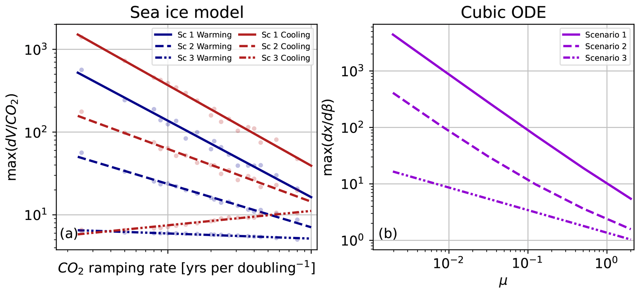
Figure 3 Maximum gradient of sea ice effective thickness with respect to CO₂ in (a) and the maximum gradient of x with respect to the forcing parameter β in (b) during transient simulations. For the sea ice model (a) the data points from the 18 different runs are shown as faded points, with a superimposed line of best fit. For the cubic ODE (b) the maximum gradient lines corresponding to increasing and decreasing forcing time series are identical due to the symmetry around β=0 seen in Fig. 1b, d, and f.

In Fig. 3a, we plot the maximum gradient of March sea ice thickness with respect to CO₂ during each hysteresis experiment, as a function of the CO₂ ramping rate. In Scenarios 1 and 2 (wide and narrow bistability, respectively), the maximum gradient gets greater as the ramping rate is slower (Fig. 3a, negative slopes of solid and dashed lines), consistent with Fig. 2 (e.g., steepening from dark-blue to light-blue curves in Fig. 2a and b). In particular, the gradient approximately follows a negative power law as a function of ramping rate on both warming and cooling time series. In Scenario 3, the maximum gradient is nearly insensitive to the ramping rate (relatively flat dash-dotted lines seen in Fig. 3a). In Fig. 3b, we see a similar result for the simple ODE, as seen by the shallowing of the power law from Scenarios 1 to 3 (though here the slope in Scenario 3 is clearly nonzero). Notably, in the cubic ODE the power law in the case with the largest region of bistability (Scenario 1) is approximately given by $\text{max}(\mathrm{d}x/\mathrm{d}\mathit{\beta })\propto {\mathit{\mu }}^{-\mathrm{1}}$, where μ again is the ramping rate. The Supplement further explains the above convergence rate of µ⁻¹.

A dependence on the reciprocal of the ramping rate in the case of wide bistability suggests that running a climate model with twice as gradual CO₂ ramping leads to a less than a factor of 2 increase in the gradient $\text{max}(\mathrm{d}V/\mathrm{d}{\mathrm{CO}}_{\mathrm{2}})$. This is an important result because this implies that the distance between the CO₂ at the simulated transient tipping point and the CO₂ of the true (equilibrium) tipping point (which we want to estimate) also only reduces by a factor of 2 when the ramping rate is reduced by a factor of 2. A greater power law slope (e.g., a slope of −2) would imply a much faster convergence to the equilibrium location of the tipping point. Thus, using more and more gradual ramping experiments may be an inefficient way to approach the equilibrium behavior of this physical system, suggesting the need for a more efficient approach, discussed next.

3.3 Predicting the steady-state behavior of sea ice using only transient runs

Our main novel result, presented next, is a method for finding the CO₂ concentration at which a bifurcation (if any) occurs in the equilibrium using computationally feasible transient model runs instead of fixed-forcing steady-state runs. We are interested in this CO₂ concentration because it determines the threshold beyond which significant sea ice loss is practically irreversible (Ritchie et al., 2021). In our simple, inexpensive model, we can test the estimates of the bistability and associated tipping points derived from transient model runs against the known true tipping points and equilibrium structure that are found from fixed-forcing runs (see Methods). When used in a GCM, our method would provide a prediction for the existence and location of tipping points when the equilibrium value of sea ice is actually unknown. Thus, this section is a proof of concept that our new method can accurately determine whether observed rate-dependent hysteresis is caused by lag around a system with no bistability or tipping points or is caused by a rate-dependent widening of an equilibrium hysteresis loop in a system with tipping points.

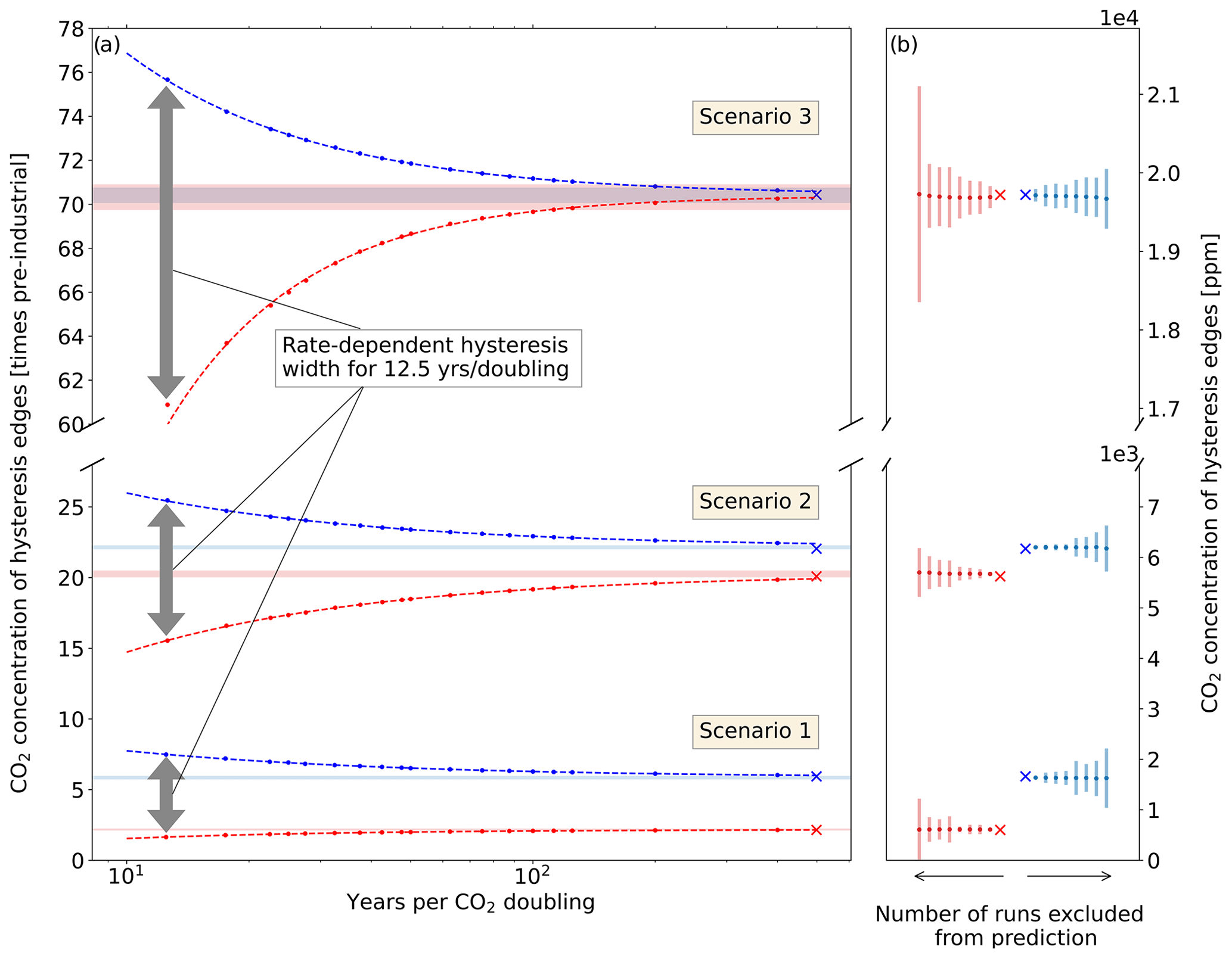
Figure 4 Estimating the equilibrium tipping point value from the rate-dependent hysteresis runs. In (a), the scatter points show the CO₂ value of the right and left edges of the rate-dependent hysteresis (${\mathrm{CO}}_{\mathrm{2}}^{\mathrm{i}}$ and ${\mathrm{CO}}_{\mathrm{2}}^{\mathrm{d}}$, located along increasing (blue) and decreasing (red) CO₂ time series, respectively) for different ramping rates. The dashed lines show the curve that is fitted to the scatter points, and the shaded blue and red bands show ± 2σ around the predicted values of ${\mathrm{CO}}_{\mathrm{2}}^{\mathrm{i}}$ and ${\mathrm{CO}}_{\mathrm{2}}^{\mathrm{d}}$ at infinitely slow ramping rates. The blue and red x symbols show the true equilibrium values of ${\mathrm{CO}}_{\mathrm{2}}^{\mathrm{i}}$ and ${\mathrm{CO}}_{\mathrm{2}}^{\mathrm{d}}$ (calculated from the fixed-CO₂ runs starting with cold and warm initial conditions, respectively). In (b), we analyze the accuracy of this prediction as we use fewer transient runs. For the three scenarios, we show the result of sequentially excluding the most gradual ramping simulations from the curve-fitting process used for predictions. The dots and the corresponding bars represent the predicted equilibrium values of ${\mathrm{CO}}_{\mathrm{2}}^{\mathrm{i}}$ and ${\mathrm{CO}}_{\mathrm{2}}^{\mathrm{d}}$, with ±2σ around the prediction, and dots moving away from the true value with larger error bars correspond to excluding more and more runs from the calculation.

In Fig. 4a, we plot a measure of the upper and lower CO₂ values that correspond to the rightmost and leftmost edges of the rate-dependent hysteresis (by calculating the CO₂ at which the March sea ice area crosses a critical threshold; see Methods and Fig. S9). We plot this measure for the warming (increasing greenhouse concentration) trajectories in blue (${\mathrm{CO}}_{\mathrm{2}}^{\mathrm{i}}$) and for the cooling (decreasing greenhouse) trajectories in red (${\mathrm{CO}}_{\mathrm{2}}^{\mathrm{d}}$), as a function of the ramping rate for all three scenarios. As expected, as the ramping rate gets slower ${\mathrm{CO}}_{\mathrm{2}}^{\mathrm{i}}$ and ${\mathrm{CO}}_{\mathrm{2}}^{\mathrm{d}}$ approach the CO₂ values corresponding to the edges of the equilibrium hysteresis and the location of the true tipping points in the case of Scenarios 1 and 2 (denoted by the × symbols). In Scenario 3, ${\mathrm{CO}}_{\mathrm{2}}^{\mathrm{i}}$ and ${\mathrm{CO}}_{\mathrm{2}}^{\mathrm{d}}$ approach the same value (the rate-dependent hysteresis width approaches zero) because there is no bistability in the steady state.

Finally, we demonstrate that fitting a curve to the edges of the rate-dependent hysteresis (${\mathrm{CO}}_{\mathrm{2}}^{\mathrm{i}}$ and ${\mathrm{CO}}_{\mathrm{2}}^{\mathrm{d}}$) as a function of the ramping rate can be used to predict ${\mathrm{CO}}_{\mathrm{2}}^{\mathrm{i}}$ and ${\mathrm{CO}}_{\mathrm{2}}^{\mathrm{d}}$ at infinitely slow ramping rates (i.e., the edges of the equilibrium hysteresis). This would allow us to estimate the CO₂ value corresponding to a bifurcation in the equilibrium behavior without running a model to a steady state. In Fig. 4a, we plot ${\mathrm{CO}}_{\mathrm{2}}^{\mathrm{i}}$ and ${\mathrm{CO}}_{\mathrm{2}}^{\mathrm{d}}$ and the curves that fit them (see Methods) as functions of the ramping rate and the predicted values of ${\mathrm{CO}}_{\mathrm{2}}^{\mathrm{i}}$ and ${\mathrm{CO}}_{\mathrm{2}}^{\mathrm{d}}$ at infinitely slow ramping rates with a 95 % confidence interval range shaded around them. We perform this fitting and estimation process using all the ramping experiments (18 different ramping rates total, as shown in Fig. 4a). We then repeat the fit using fewer and fewer experiments to explore how the uncertainty in predicted values of ${\mathrm{CO}}_{\mathrm{2}}^{\mathrm{i}}$ and ${\mathrm{CO}}_{\mathrm{2}}^{\mathrm{d}}$ increases as we move to only using a few fast ramping experiments that are more feasible when using full-complexity climate models. Figure 4b shows a summary of these analyses.

The predicted values of ${\mathrm{CO}}_{\mathrm{2}}^{\mathrm{i}}$ and ${\mathrm{CO}}_{\mathrm{2}}^{\mathrm{d}}$ are remarkably accurate for all scenarios (points approaching the red and blue x symbols in Fig. 4b), even when excluding several of the slower ramping experiments. This is an important test because when this method is applied to a GCM, one would only have a smaller number of faster-ramping experiments due to computational limitations. The uncertainties (indicated by the shaded blue and red bars around the points) in the predictions grow when excluding more experiments from the curve fitting process but still remain very low, especially for Scenarios 1 and 2. In predicting ${\mathrm{CO}}_{\mathrm{2}}^{\mathrm{d}}$ for Scenario 3, the uncertainties are a bit higher because the functional form of our fit does not represent this case as well as the others, leading to serial correlation in the residuals. The structure in the residuals can be used to guide the choice of the functional form used to fit such model output in future applications. This same method and functional form can also successfully predict the equilibrium structure of our simple ODE (Eq. 1), with even smaller uncertainties in the prediction when using very few ramping experiments (see Fig. S11). Finally, we can use the difference between the distributions ${\mathrm{CO}}_{\mathrm{2}}^{\mathrm{i}}$ and ${\mathrm{CO}}_{\mathrm{2}}^{\mathrm{d}}$ to calculate the probability that bistability – and thus a tipping point – exists (see the Supplement). Another very similar approach using only the difference between ${\mathrm{CO}}_{\mathrm{2}}^{\mathrm{i}}$ and ${\mathrm{CO}}_{\mathrm{2}}^{\mathrm{d}}$ (i.e., the hysteresis width) as a function of the ramping rate is also shown in Fig. S10.

Overall, these results demonstrate the potential for using several shorter runs with time-changing CO₂ forcing to efficiently estimate the CO₂ value of the tipping points and predict the existence of bistability in GCMs where equilibrium runs or long, slow-ramping hysteresis runs are computationally infeasible.

4 Discussion

We have shown that a single climate model hysteresis run with time-changing (transient) forcing cannot be used to conclusively estimate the true location of Arctic winter sea ice tipping points, the range of bistability in the steady state, and even the existence of bistability at all. We demonstrated that the transient sea ice responses under time-changing CO₂ reflect the generic behavior of a nonlinear dynamical system (e.g., our Eq. 1): specifically, we showed that systems with and without bistability can also produce qualitatively indistinguishable rate-dependent hysteresis behavior. We also find that very long model runs are needed to identify whether the system approaches a bifurcation (Fig. 3) and at what CO₂ this occurs. We showed that even in runs with a very slow-changing CO₂, the system can be surprisingly far from the equilibrium as it undergoes a tipping point, consistent with the work of Li et al. (2013). In addition, even with a very slow-ramping experiment, one would always have to perform additional expensive fixed-forcing experiments (as done by Li et al., 2013) to confirm that the experiment was indeed in quasi-equilibrium. Instead, we propose a novel method that uses a few fast-ramping experiments to efficiently predict the true range of bistability and provide uncertainty estimates on this prediction.

We demonstrated that the method we propose can accurately predict the steady-state behavior of sea ice in a simple model; now we discuss applying this method to a GCM. First, we note that while we use a highly idealized model of sea ice in this study, the method developed deals with identifying bistability in complex systems with unknown equilibrium structures more generally. This means that the framework should be applicable to other models (including GCMs), since moving from fast- to slower-ramping rates allows convergence to the equilibrium behavior. It could also be used in the context of vastly different climate problems, for example, in identifying the abrupt transitions to a moist greenhouse (Popp et al., 2016), runaway greenhouse (Goldblatt et al., 2013), or snowball Earth state (Hyde et al., 2000). The functional form used to fit the transient runs, as well as the level of certainty achieved from a given number of experiments, would likely depend on the given model and climate problem analyzed. Possible challenges in finding the functional best fit to the transient runs might mirror those of Gregory et al. (2004), who encountered difficulties when trying to fit a line to un-equilibrated GCM runs with a different goal of deducing the equilibrium climate sensitivity. We suggest that a careful examination of the residuals from a given fit can help guide the choice of functional form.

The generality of the method also highlights another advantage: the same set of ramping experiments in a GCM could be used to analyze all suspected tipping elements in the Earth's climate system simultaneously. The main challenge we anticipate in applying this method to GCMs comes from the significant stochastic variability and multiple timescales of forcings that may render the calculated width of the rate-dependent hysteresis more uncertain in a GCM. Nonetheless, using multiple runs to estimate the width of the bistability of a given climate variable and providing a quantified uncertainty in such a prediction should offer a potential improvement over using a single hysteresis experiment.

We can estimate the efficiency of the proposed approach over more standard ones when applied in a GCM. Taking the experimental setup of Li et al. (2013) as a guide, we can assume that a slow-ramping experiment to four times CO₂ requires a 2000-year ramp-up and ramp-down with at minimum a 2500-year equilibration period after each ramp (though they actually allowed the model to equilibrate for nearly 6000 years). Within the 500 ppm width of the rate-dependent hysteresis found by Li et al. (2013), 10 fixed-forcing experiments 2500 years long would be needed to test for bistability and estimate the tipping point location at a relatively crude accuracy of 100 ppm. This leads to a total of 34 000 simulation years. On the other hand, if we used our proposed approach, we could run three ramping experiments with fast to intermediate rates of 100, 200, and 400 years to quadruple CO₂. We would run only one experiment to complete equilibration after ramp-up (2500 years) and run the others only until they lost their sea ice, using the ice-free steady-state run to conduct the three ramp-downs. This yields a total of approximately 6400 simulation years and computational savings of over a factor of 5. Using only three ramping experiments is sufficient to get an estimate of the equilibrium hysteresis width and location, but the uncertainty in the estimate could still be high.

Finally, our results indicate that rate-dependent hysteresis and irreversibility of Arctic winter sea ice are expected to be relevant for realistic rates of CO₂ increase. While rate-dependent hysteresis has been explored in other climate contexts (e.g., AMOC; Kim et al., 2021; An et al., 2021), previous work on Arctic winter sea ice has typically sought to identify equilibrium hysteresis in sea ice because it would imply irreversibility of sea ice loss, generally ignoring the out-of-equilibrium behavior of sea ice under rapid CO₂ changes. The SSP585 scenario in CMIP6 corresponds to a ramping rate of approximately 60 years per CO₂ doubling; this is a rate at which sea ice in our idealized model already exhibits rate-dependent hysteresis and significant deviation from its steady state (see Figs. 2 and S2). Since we identify rate-dependent hysteresis in sea ice here in all scenarios, even without a deep ocean and subsequent recalcitrant warming (Held et al., 2010), we expect rate-dependent hysteresis to be even more pronounced in GCMs and in the real climate when such long-timescale components are included. We, therefore, conclude that on policy-relevant timescales the significant irreversibility of winter Arctic sea ice involved in rate-dependent hysteresis is likely to occur in the real climate system due to the expected lagged response regardless of whether an actual bifurcation (tipping point) in the equilibrium exists.