the Creative Commons Attribution 4.0 License.
the Creative Commons Attribution 4.0 License.
 | 15 Jan 2021
Fast hybrid tempered ensemble transform filter formulation for Bayesian elliptical problems via Sinkhorn approximation
Sangeetika Ruchi
Svetlana Dubinkina
Identification of unknown parameters on the basis of partial and noisy data is a challenging task, in particular in high dimensional and non-linear settings. Gaussian approximations to the problem, such as ensemble Kalman inversion, tend to be robust and computationally cheap and often produce astonishingly accurate estimations despite the simplifying underlying assumptions. Yet there is a lot of room for improvement, specifically regarding a correct approximation of a non-Gaussian posterior distribution. The tempered ensemble transform particle filter is an adaptive Sequential Monte Carlo (SMC) method, whereby resampling is based on optimal transport mapping. Unlike ensemble Kalman inversion, it does not require any assumptions regarding the posterior distribution and hence has shown to provide promising results for non-linear non-Gaussian inverse problems. However, the improved accuracy comes with the price of much higher computational complexity, and the method is not as robust as ensemble Kalman inversion in high dimensional problems. In this work, we add an entropy-inspired regularisation factor to the underlying optimal transport problem that allows the high computational cost to be considerably reduced via Sinkhorn iterations. Further, the robustness of the method is increased via an ensemble Kalman inversion proposal step before each update of the samples, which is also referred to as a hybrid approach. The promising performance of the introduced method is numerically verified by testing it on a steady-state single-phase Darcy flow model with two different permeability configurations. The results are compared to the output of ensemble Kalman inversion, and Markov chain Monte Carlo methods results are computed as a benchmark.
- Article
(3416 KB) - Full-text XML
- BibTeX
- EndNote


If a solution of a considered partial differential equation (PDE) is highly sensitive to its parameters, accurate estimation of the parameters and their uncertainties is essential to obtain a correct approximation of the solution. Partial observations of the solution are then used to infer uncertain parameters by solving a PDE-constrained inverse problem. For instance, one can approach such problems via methods induced by Bayes' formula (Stuart, 2010). More specifically, the posterior probability density of the parameters given the data is then computed on the basis of a prior probability density and a likelihood, which is the conditional probability density associated with the given noisy observations. The well-posedness of an inverse problem and convergence to the true posterior in the limit of observational noise going to zero were proven for different priors and under assumptions on the parameter-to-observation map by Dashti and Stuart (2017), for example.
When aiming at practical applications as in oil reservoir management (Lorentzen et al., 2020) and meteorology (Houtekamer and Zhang, 2016), for example, the posterior is approximated by means of a finite set of samples. Markov chain Monte Carlo (MCMC) methods approximate the posterior with a chain of samples – a sequential update of samples according to the posterior (Robert and Casella, 2004; Rosenthal, 2009; Hoang et al., 2013). Typically, MCMC methods provide highly correlated samples. Therefore, in order to sample the posterior correctly, MCMC requires a long chain, especially in the case of a multi-modal or a peaked distribution. A peaked posterior is associated with very accurate observations. Therefore, unless a speed-up is introduced in a MCMC chain (e.g. Cotter et al., 2013), MCMC is impractical for computationally expensive PDE models.
Adaptive Sequential Monte Carlo (SMC) methods are different approaches to approximate the posterior with an ensemble of samples by computing their probability (e.g, Vergé et al., 2015). Adaptive intermediate probability measures are introduced between the prior measure and the posterior measure to improve upon method divergence due to the curse of dimensionality following Del Moral et al. (2006) and Neal (2001). Moreover, sampling from an invariant Markov kernel with the target intermediate measure and the reference prior measure improves upon ensemble diversity due to parameters' stationarity, as shown by Beskos et al. (2015). However, when parameter space is high dimensional, adaptive SMC requires computationally prohibitive ensemble sizes unless we approximate only the first two moments (e.g. Iglesias et al., 2018) or we sample highly correlated samples (Ruchi et al., 2019).
Ensemble Kalman inversion (EKI) approximates primarily the first two moments of the posterior, which makes it computationally attractive for estimating high dimensional parameters (Iglesias et al., 2014). For linear problems, Blömker et al. (2019) showed well-posedness and convergence of the EKI for a fixed ensemble size and without any assumptions of Gaussianity. However for non-linear problems, it has been shown by Oliver et al. (1996), Bardsley et al. (2014), Ernst et al. (2015), Liu et al. (2017) and Le Gland et al. (2009) that the EKI approximation is not consistent with the Bayesian approximation.
We note that the EKI is an iterative ensemble smoother (Evensen, 2018). Iterative ensemble smoothers for inverse problems introduce a trivial artificial dynamics to the unknown static parameter and iteratively update an estimation of the parameter. Then the parameter-dependent model variables are recomputed using a forward model with a parameter estimation. Examples of iterative ensemble smoothers are ensemble randomised maximum likelihood (Chen and Oliver, 2012), multiple data assimilation (Emerick and Reynolds, 2013) and randomise-then-optimise (Bardsley et al., 2014).
As an alternative ansatz one can employ optimal transport resampling that lies at the heart of the ensemble transform particle filter (ETPF) proposed by Reich (2013). An optimal transport map between two consecutive probability measures provides a direct sample-to-sample map with maximised sample correlation. Along the lines of an adaptive SMC approach, a probability measure is described via the importance weights, and the deterministic mapping replaces the traditional resampling step. A so-called tempered ensemble transform particle filter (TETPF) was proposed by Ruchi et al. (2019). Note that this ansatz does not require any distributional assumption for the posterior, and it was shown by Ruchi et al. (2019) that the TETPF provides encouraging results for non-linear high dimensional PDE-constrained inverse problems. However, the computational cost of solving an optimal transport problem in each iteration is considerably high.
In this work we address two issues that have arisen in the context of the TETPF: (i) the immense computational costs of solving the associated optimal transport problem and (ii) the lack of robustness of the TETPF with respect to high dimensional problems. More specifically, the performance of ETPF has been found to be highly dependent on the initial guess. Although tempering restrains any sharp fail in the importance sampling step due to a poor initial ensemble selection, the number of required intermediate steps and the efficiency of ETPF still depend on the initialisation. The lack of robustness in high dimensions can be addressed via a hybrid approach that combines a Gaussian approximation with a particle filter approximation (e.g. Santitissadeekorn and Jones, 2015). Different algorithms are created by Frei and Künsch (2013) and Stordal et al. (2011), for example. In this paper, we adapt a hybrid approach of Chustagulprom et al. (2016) that uses the EKI as a proposal step for the ETPF with a tuning parameter. Furthermore, it is well established that the computational complexity of solving an optimal transport problem can be significantly reduced via a Sinkhorn approximation by Cuturi (2013). This ansatz has been implemented for the ETPF by Acevedo et al. (2017).
Along the lines of Chustagulprom et al. (2016) and de Wiljes et al. (2020), we propose a tempered ensemble transform particle filter with Sinkhorn approximation (TESPF) and a tempered hybrid approach.
The remainder of the paper is organised as follows: in Sect. 2, the inverse problem setting is presented. There we describe the tempered ensemble transform particle filter (TETPF) proposed by Ruchi et al. (2019). Furthermore, we introduce the tempered ensemble transform particle filter with Sinkhorn approximation (TESPF), a tempered hybrid approach that combines the EKI and the TETPF (hybrid EKI–TETPF), and a tempered hybrid approach that combines the EKI and the TESPF (hybrid EKI–TESPF). We provide pseudocodes of all the presented techniques in Appendix A and corresponding computational complexities in Appendix B. In Sect. 3, we apply the adaptive SMC methods to an inverse problem of inferring high dimensional permeability parameters for a steady-state single-phase Darcy flow model. Permeability is parameterised following Ruchi et al. (2019), whereby one configuration of parameterisation leads to Gaussian posteriors, while another one leads to non-Gaussian posteriors. Finally, we draw conclusions in Sect. 4.
We assume is a random variable that is related to partially observable quantities by a non-linear forward operator , namely
Further, yobs∈𝒴 denotes a noisy observation of y, i.e.
where and 𝒩(0,R) is a Gaussian distribution with zero mean and R covariance matrix. The aim is to determine or approximate the posterior measure μ(u) conditioned on observations yobs and given a prior measure μ0(u), which is referred to as a Bayesian inverse problem. The posterior measure is absolutely continuous with respect to the prior, i.e.
where ∝ is up to a constant of normalisation, and g is referred to as the likelihood and depends on the forward operator G. The Gaussian observation noise of the observation yobs implies
where ′ denotes the transpose. In the following we will introduce a range of methods that can be employed to estimate solutions to the presented inverse problem under the overarching mantel of tempered Sequential Monte Carlo filters. Alongside these methods we will also propose several important add-on tools required to achieve feasibility and higher accuracy in high dimensional non-linear settings.
2.1 Tempered Sequential Monte Carlo
We consider Sequential Monte Carlo (SMC) methods that approximate the posterior measure μ(u) via an empirical measure
Here, δ is the Dirac function, and the importance weights for the approximation of μ are
An ensemble consists of M realisations ui∈ℝn of a random variable u that are independent and identically distributed according to ui∼μ0.
When an easy-to-sample ensemble from the prior μ0 does not approximate the complex posterior μ well, only a few weights wi have significant value, resulting in a degenerative approximation of the posterior measure. Potential reasons for this effect are high dimensionality of the uncertain parameter, a large number of observations, or lack of accuracy of the observations. An existing solution to a degenerative approximation is an iterative approach based on tempering by Del Moral et al. (2006) or annealing by Neal (2001). The underlying idea is to introduce T intermediate artificial measures between μ0 and μt=μ. These measures are bridged by introducing T tempering parameters that satisfy . An intermediate measure μt is defined as a probability measure that has density proportional to g(u) with respect to the previous measure μt−1:
Along the lines of Iglesias (2016) the tempering parameter ϕt is chosen such that the effective sample size (ESS),
with
does not drop below a certain threshold 1<Mthresh<M. Then, an approximation of the posterior measure μt is
A bisection algorithm on the interval is employed to find ϕt. If ESSt>Mthresh, we set ϕT=1, which implies that no further tempering is required.
The choice of ESS to define a tempering parameter is supported by results of Beskos et al. (2014) on the stability of a tempered SMC method in terms of the ESS. Moreover, for a Gaussian probability density approximated by importance sampling, Agapiou et al. (2017) showed that ESS is related to the second moment of the Radon–Nikodym derivative (Eq. 1).
The SMC method with importance sampling (Eq. 4) does not change the sample , which leads to the method collapse due to a finite ensemble size. Therefore each tempering iteration t needs to be supplied with resampling. Resampling provides a new ensemble that approximates the measure μt. We will discuss different resampling techniques in Sect. 2.3.
2.2 Mutation
Due to the stationarity of the parameters, SMC methods require ensemble perturbation. In the framework of particle filtering for dynamical systems, ensemble perturbation is achieved by rejuvenation, when ensemble members of the posterior measure are perturbed with a random noise sampled from a Gaussian distribution with zero mean and a covariance matrix of the prior measure. The covariance matrix of the ensemble is inflated, and no acceptance step is performed due to the associated high computational costs for a dynamical system.
Since we consider a static inverse problem, for ensemble perturbation we employ a Metropolis–Hastings method (thus we mutate samples) but with a proposal that speeds up the MCMC method for estimating a high dimensional parameter. Namely, we use the ensemble mutation of Cotter et al. (2013) with the target measure μt and the reference measure μ0. The mutation phase is initialised at , and at the final inner iteration τmax, we assign for .
For a Gaussian prior we use the preconditioned Crank–Nicolson MCMC (pcn-MCMC) method:
Here, m is the mean of the Gaussian prior measure μ0, and are from a Gaussian distribution with zero mean and a covariance matrix of the Gaussian prior measure μ0.
For a uniform prior U[a,b] we use the following random walk:
Here and are projected onto the [a,b] interval if necessary. Then the ensemble at the inner iteration τ+1 is
Here is from Eq. (5) for the Gaussian measure and from Eq. (6) for the uniform measure, and
The scalar in Eq. (5) controls the performance of the Markov chain. Small values of θ lead to high acceptance rates but poor mixing. Roberts and Rosenthal (2001) showed that for high dimensional problems it is optimal to choose θ such that the acceptance rate is in between 20 % and 30 % by the last tempering iteration T. Cotter et al. (2013) proved that under some assumptions this mutation produces a Markov kernel with an invariant measure μt.
Computational complexity. In each tempering iteration t the computational complexity of the pcn-MCMC mutation is 𝒪(τmaxM𝒞), where 𝒞 is the computational cost of the forward model G. For the pseudocode of the pcn-MCMC mutation, please refer to Algorithm 1 in Appendix A. Note that the computational complexity is not affected by the length of u, which is a very desirable property in high dimensions as shown by Cotter et al. (2013) and Hairer et al. (2014).
2.3 Resampling phase
As we have already mentioned in Sect. 2.1, an adaptive SMC method with importance sampling needs to be supplied with resampling at each tempering iteration t. We consider a resampling method based on optimal transport mapping proposed by Reich (2013).
2.3.1 Optimal transformation
The origin of the optimal transport theory lies in finding an optimal way of redistributing mass which was first formulated by Monge (1781). Given a distribution of matter, e.g. a pile of sand, the underlying question is how to reshape the matter into another form such that the work done is minimal. A century and a half later the original problem was rewritten by Kantorovich (1942) in a statistical framework that allowed it to be tackled. Due to these contributions it was later named the Monge–Kantorovich minimisation problem. The reader is also referred to Peyré and Cuturi (2019) for a comprehensible overview.
Let us consider a scenario whereby the initial distribution of matter is represented by a probability measure μ on the measurable space 𝒰, that has to be moved and rearranged according to a given new distribution ν, defined on the measurable space . In order to describe the link between the two probability measures μ and ν and to minimise a predefined cost associated with the transportation, one aims to find a joint measure on that is a solution to
where the minimum is computed over all joint probability measures ω on , denoted , with marginals μ and ν, and is a transport cost function on . The joint measures achieving the infinum are called optimal transport plans.
Let μ and ν be two measures on a measurable space (Ω,ℱ) such that μ is the law of random variable and ν is the law of random variable . Then a coupling of (μ,ν) consists of a pair . Note that couplings always exist; an example is the trivial coupling in which the random variables U and are independent. A coupling is called deterministic if there is a measurable function such that , and ΨM is called a transport map. Unlike general couplings, deterministic couplings do not always exist. On the other hand there may be infinitely many deterministic couplings. One famous variant of Eq. (9), whereby the optimal coupling is known to be a deterministic coupling, is given by
The aim of the resampling step is to obtain equally probable samples. Therefore, in resampling based on optimal transport of Reich (2013), the Monge–Kantorovich minimisation problem (Eq. 10) is considered for the current posterior measure given by its samples approximation (Eq. 4) and a uniform measure (here the weights in the sample approximation are set to 1∕M). The discretised objective functional of the associate optimal transport problem is given by
subject to sij>0 and constraints
where matrix S describes a joint probability measure under the assumption that the state space is finite. Then samples are obtained by a deterministic linear transform, i.e.
Reich (2013) showed weak convergence of the deterministic optimal transformation (Eq. 11) to a solution of the Monge–Kantorovich problem (Eq. 9) as M→∞.
Computational complexity. The computational complexity of solving the optimal transport problem with an efficient earth mover's distance algorithm such as FastEMD of Pele and Werman (2009) is of order 𝒪(M3log M). Consequently the computational complexity of the adaptive tempering SMC with optimal transport resampling (TETPF) is , where T is the number of tempering iterations, τmax is the number of pcn-MCMC inner iterations and 𝒞 is the computational cost of a forward model G. For the pseudocode of the TETPF, please refer to Algorithm 2 in Appendix A.
2.3.2 Sinkhorn approximation
As discussed above, solving the optimal transport problem has a computational complexity of 𝒪=M3log (M) in every iteration of the tempering procedure. Thus the TETPF becomes very expensive for large M. On the other hand an increase in the number of samples directly correlates with an improved accuracy of the estimation. In order to allow for as many samples as possible, one needs to reduce the associated computational cost of the optimal transport problem. This can be achieved by replacing the optimal transport distance with a Sinkhorn distance and subsequently exploiting the new structure to elude the immense computational time of the EMD (Earth mover's distance) solver, as shown by Cuturi (2013). More precisely the ansatz is built on the fact that the original transport problem has a natural entropic bound that is obtained for , where and , which constitutes an independent joint probability. Therefore, one can consider the problem of finding a matrix that is constrained by an additional lower entropic bound (Sinkhorn distance). This additional constraint can be incorporated via a Lagrange multiplier, which leads to the above regularised form, i.e.
where α>0. Due to additional smoothness the minimum of Eq. (12) can be unique and has the form
where Z is a matrix with entries and b and a non-negative vectors determined by employing Sinkhorn's fixed point iteration described by Sinkhorn (1967). We will refer to this approach as the tempered ensemble Sinkhorn particle filter (TESPF).
Computational complexity. Solving this regularised optimal transport problem rather than the original transport problem given in Eq. (9) reduces the complexity to 𝒪(M2C(α)), where C(α) denotes a computational scaling factor that depends on the choice of the regularisation factor α. In particular C(α) grows with α. Therefore, one needs to balance between reducing computational time and finding a reasonable approximate solution of the original transport problem when choosing a value for α. For the pseudocode of the Sinkhorn adaptation of solving the optimal transport problem, please refer to Algorithm 3 in Appendix A. For the pseudocode of the TESPF, please refer to Algorithm 4 in Appendix A.
2.4 Ensemble Kalman inversion
For Bayesian inverse problems with Gaussian measures, ensemble Kalman inversion (EKI) is one of the widely used algorithms. The EKI is an adaptive SMC method that approximates primarily the first two statistical moments of a posterior distribution. For a linear forward model, the EKI is optimal in the sense that it minimises the error in the mean (Blömker et al., 2019). For a non-linear forward model, the EKI still provides a good estimation of the posterior (e.g. Iglesias et al., 2018). Here we consider the EKI method of Iglesias et al. (2018), since it is based on the tempering approach.
The intermediate measures are approximated by Gaussian distributed variables with empirical mean mt and empirical variance Ct. Empirical mean mt−1 and empirical covariance Ct−1 are defined in terms of as follows:
where ⊗ denotes the Kronecker product. Then the mean and the covariance are updated as
respectively. Here ′ denotes the transpose,
We recall that the non-linear forward problem is y=G(u), the observation yobs has a Gaussian observation noise with zero mean and the covariance matrix R and ϕt is a temperature associated with the measure μt.
Since we are interested in an ensemble approximation of the posterior distribution, we update the ensemble members by
Here and for .
Computational complexity. The computational complexity of solving Eq. (13) is 𝒪(κ2n), where n is the parameter space dimension, and κ is the observation space dimension. Then the computational complexity of the EKI is , where T is the number of tempering iterations, τmax is the number of pcn-MCMC inner iterations and 𝒞 is the computational cost of a forward model G. For the pseudocode of the EKI method, please refer to Algorithm 5 in Appendix A.
2.5 Hybrid
Despite the underlying Gaussian assumption, the EKI is remarkably robust in non-linear high dimensional settings as opposed to consistent SMC methods such as the TET(S)PF. For many non-linear problems it is desirable to have better uncertainty estimates while maintaining a level of robustness. This can be achieved by factorising the likelihood given by Eq. (2), e.g,
where
and
Then it is possible to alternate between methods with complementing properties such as the EKI and the TET(S)PF updates; e.g. likelihood,
is used for an EKI update followed by an update with a TET(S)PF on the basis of
Note that and should be tuned according to the underlying forward operator. This combination of an approximative Gaussian method and a consistent SMC method has been referred to as hybrid filters in the data assimilation literature1(Stordal et al., 2011; Frei and Künsch, 2013; Chustagulprom et al., 2016). This ansatz can also be understood as using the EKI as a more elaborate proposal density for the importance sampling step within SMC (e.g. Oliver et al., 1996).
Computational complexity. The computational complexity of combining the two algorithms is for the hybrid EKI–TETPF and for the hybrid EKI–TESPF. For the pseudocode of the hybrid methods, please refer to Algorithm 6 in Appendix A.
We consider a steady-state single-phase Darcy flow model defined over an aquifer of a two-dimensional physical domain , which is given by
where , ⋅ the dot product, P(x,y) the pressure, k(x,y) the permeability, f(x,y) the source term which accounts for groundwater recharge and (x,y) the horizontal dimensions. The boundary conditions are
where ∂D is the boundary of domain D. The source term is
We implement a cell-centred finite-difference method and a linear algebra solver (backslash operator in MATLAB) to solve the forward model (Eqs. 16–17) on an N×N grid.
We note that a single-phase Darcy flow model, though not a steady-state model, is widely used to model the flow in a subsurface aquifer and to infer uncertain permeability using data assimilation. For example, Zovi et al. (2017) used an EKI to infer permeability of an existing aquifer located in north-east Italy. The area of this aquifer is 2.7 km2 and exhibits several channels, such as the one depicted in Fig. 1. There, a size of a computational cell ranged from 2 m (near wells) to 20 m away from the wells.
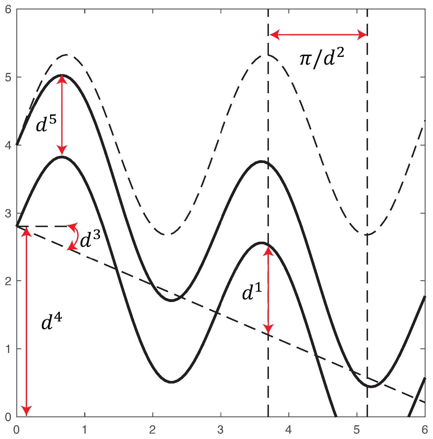
Figure 1Geometrical configuration of channel flow: amplitude d1, frequency d2, angle d3, initial point d4 and width d5.
3.1 Parameterisation of permeability
We consider the following two parameterisations of the permeability function k(x,y):
-
F1: log permeability over the entire domain D, ;
-
F2: permeability over domain D that has a channel, as by Iglesias et al. (2014).
Here Dc denotes a channel, δ is the Dirac function and and denote permeabilities inside and outside the channel. The geometry of the channel is parameterised by five parameters : amplitude, frequency, angle, initial point and width, correspondingly. The lower boundary of the channel is given by . The upper boundary of the channel is given by y+d5. These parameters are depicted in Fig. 1.
We assume that the log permeability for both F1 and F2 is drawn from a Gaussian distribution with mean m and covariance C. We define C via a correlation function given by the Whittle–Matern correlation function defined by Matérn (1986):
where γ is the gamma function, υ=0.5 is the characteristic length scale and Υ1 is the modified Bessel function of the second kind of order 1.
With λ and V we denote eigenvalues and eigenfunctions of the corresponding covariance matrix C, respectively. Then, following a Karhunen–Loève (KL) expansion, log permeability is
where uℓ is i.i.d. from 𝒩(0,1) for .
For F1, the prior for log permeability is a Gaussian distribution with mean 5. The grid dimension is N=70, and thus the uncertain parameter has dimension 4900.
For F2, we assume geometrical parameters are drawn from uniform priors, namely d, d, d, d, d. Furthermore, we assume independence between geometric parameters and log permeability. The prior for log permeability is a Gaussian distribution with mean 15 outside the channel and with mean 100 inside the channel. The grid dimension is N=50. Log permeability inside channel and log permeability outside channel are defined over the entire domain 50×50. Therefore, for F2 inference the uncertain parameter has dimension 5005. Moreover, for F2 we use the Metropolis-within-Gibbs methodology following Iglesias et al. (2014) to separate geometrical parameters and log permeability parameters within the mutation step, since it allows the structure of the prior to be better exploited.
3.2 Observations
Both the true permeability and an initial ensemble are drawn from the same prior distribution as the prior includes knowledge about geological properties. However, an initial guess is computed on a coarse grid, and the true solution is computed on a fine grid that has twice the resolution of the coarse grid. The synthetic observations of pressure are obtained by
An element of L(Ptrue) is a linear functional of pressure, namely
Here σ=0.01, Δx2 is the size of a grid cell , Nf is the resolution of a fine grid, hj is the location of the observation and κ is the number of observations. This form of the observation functional and the parameterisation F1 and F2 guarantee the continuity of the forward map from the uncertain parameters to the observations and thus the existence of the posterior distribution, as shown by Iglesias et al. (2014). The observation noise η is drawn from a normal distribution with zero mean and known covariance matrix R. We choose the observation noise to be 2 % of L2-norm of the true pressure. With such a small noise the likelihood is a peaked distribution. Therefore, a non-iterative data assimilation approach requires a computationally unfeasible number of ensemble members to sample the posterior.
To save computational costs, we choose an ESS threshold for tempering and the length of the Markov chain τmax=20 for mutation.
3.3 Metrics
We conduct numerical experiments with ensemble sizes M=100 and M=500 and 20 simulations with different initial ensemble realisations to check the robustness of results. We analyse the method's performance with respect to a pcn-MCMC solution, from here on referred to as the reference. An MCMC solution was obtained by combining 50 independent chains each of length 106, 105 burn-in period and 103 thinning. For log permeability, we compute the root mean square error (RMSE) of the mean
and uref is the reference solution.
For geometrical parameters d, we compute the Kullback–Leibler divergence
where pref(di) is the reference posterior, p(di) is approximated by the weights and is a chosen number of bins.
3.4 Application to F1 inference
For F1, we perform numerical experiments using 36 uniformly distributed observations, which are displayed in circles in Fig. 3a. We plot a box plot of the RMSE given by Eq. (18) over 20 independent simulations in Fig. 2a using Sinkhorn approximation and in Fig. 2b using optimal transport. The horizontal axis is for the hybrid parameter β, whose value 0 corresponds to the EKI and 1 to an adaptive SMC method with either a Sinkhorn approximation (TESPF) or optimal transport (TETPF). Ensemble size M=100 is shown in red and M=500 in green. First, we observe that at a small ensemble size M=100 and a large β (namely β≥0.6), TESPF outperforms the TETPF as the RMSE is lower. Since Sinkhorn approximation is a regularisation of an optimal transport solution, the TESPF provides a smoother solution than the TETPF that can be seen in Fig. 3c and 3f, respectively, where we plot mean log permeability. Next, we see in Fig. 2 that the hybrid approach decreases the RMSE compared to TET(S)PF: the smaller the β value, the smaller the median of the RMSE. The EKI gives the smallest error due to the Gaussian parameterisation of permeability. The advantage of the hybrid approach is most pronounced at a large ensemble size of M=500 and optimal transport resampling. Furthermore, we note a discrepancy between the M=100 and the M=500 experiments at β=0, i.e. for the pure EKI. This is related to the curse of dimensionality. It appears that the ensemble size M=100 is too small to estimate an uncertain parameter of the dimension 103 using 36 accurate observations. However, at the ensemble size M=500 the EKI alone (β=0) gives an excellent performance compared to any combination (β>0).
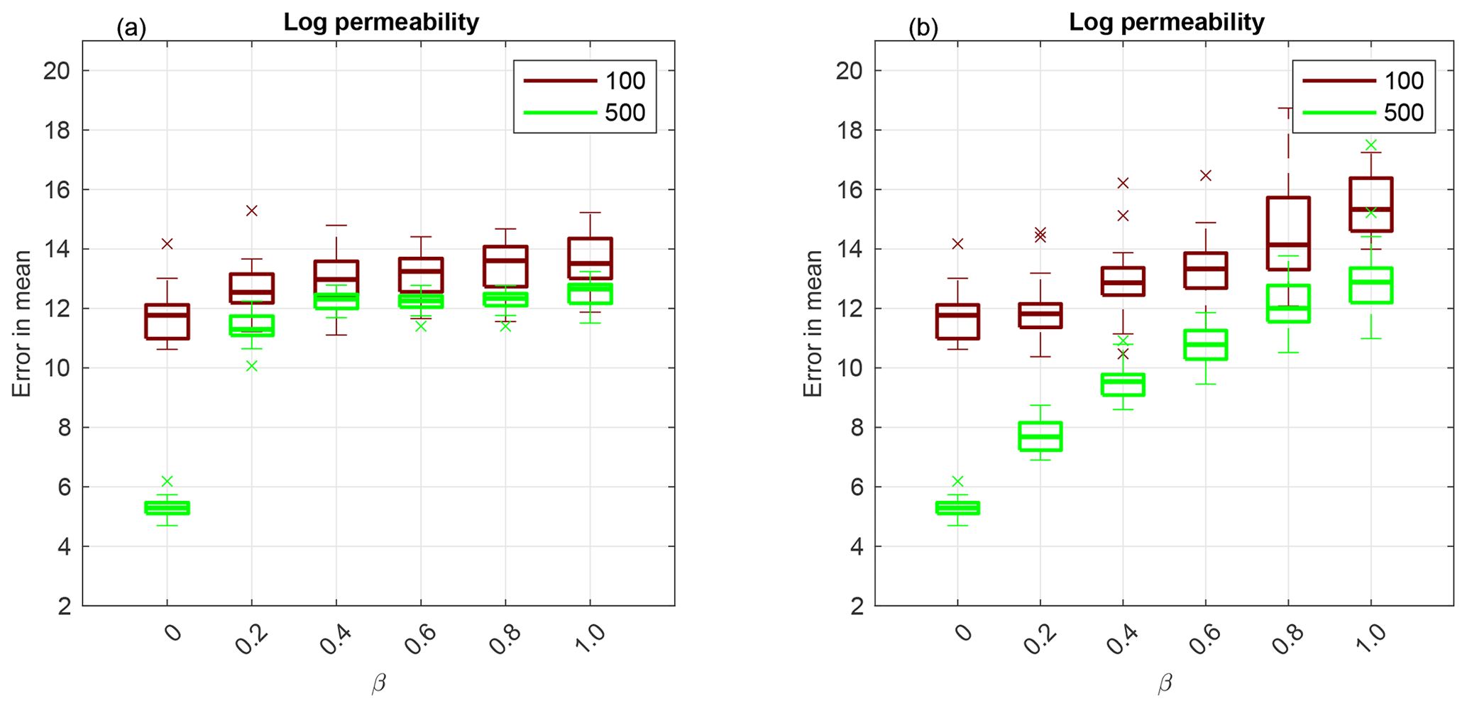
Figure 2Application to F1 parameterisation: using Sinkhorn approximation (a) and optimal transport resampling (b). Box plot over 20 independent simulations of the RMSE of mean log permeability. The horizontal axis is for the hybrid parameter, where β=0 corresponds to the EKI and β=1 to TET(S)PF. The ensemble size M=100 is shown in red and M=500 in green. The central mark is the median, the edges of the box are the 25th and 75th percentiles, whiskers extend to the most extreme data points and crosses are outliers.
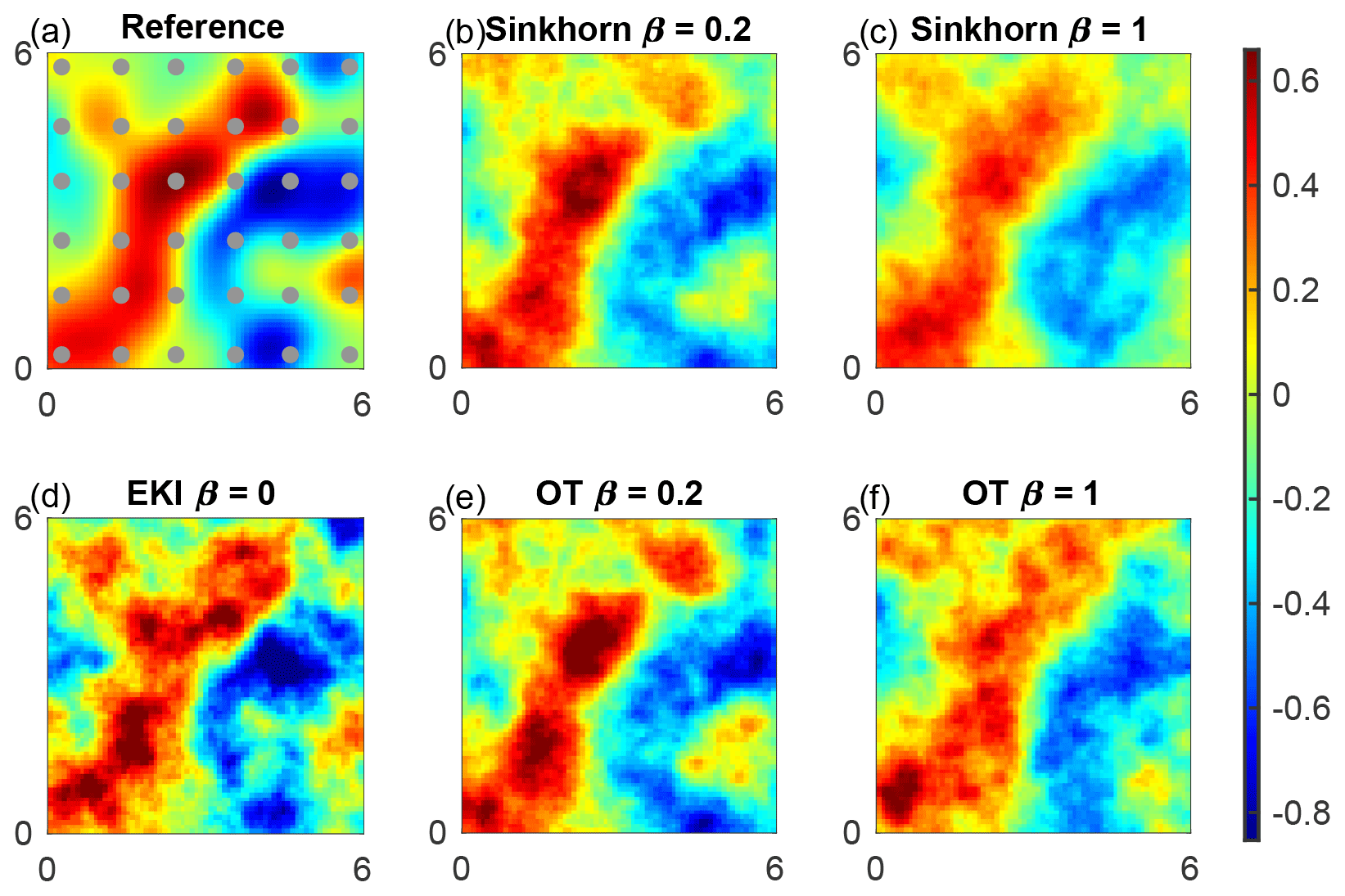
Figure 3Mean log permeability for F1 inference for the lowest error at ensemble size M=100. Observation locations are shown by circles. Reference (a), TESPF(0.2) (b), TESPF (c), EKI (d), TETPF(0.2) (e) and TETPF (f).
We plot mean log permeability at ensemble size M=100 and the smallest RMSE over 20 simulations in Fig. 3b–f and of the reference in Fig. 3a. We see that the EKI and the TETPF(0.2) estimate not only large-scale features but also small-scale features (e.g. negative mean in the top right corner) unlike the TET(S)PF and TESPF(0.2) well.
3.5 Application to F2 inference
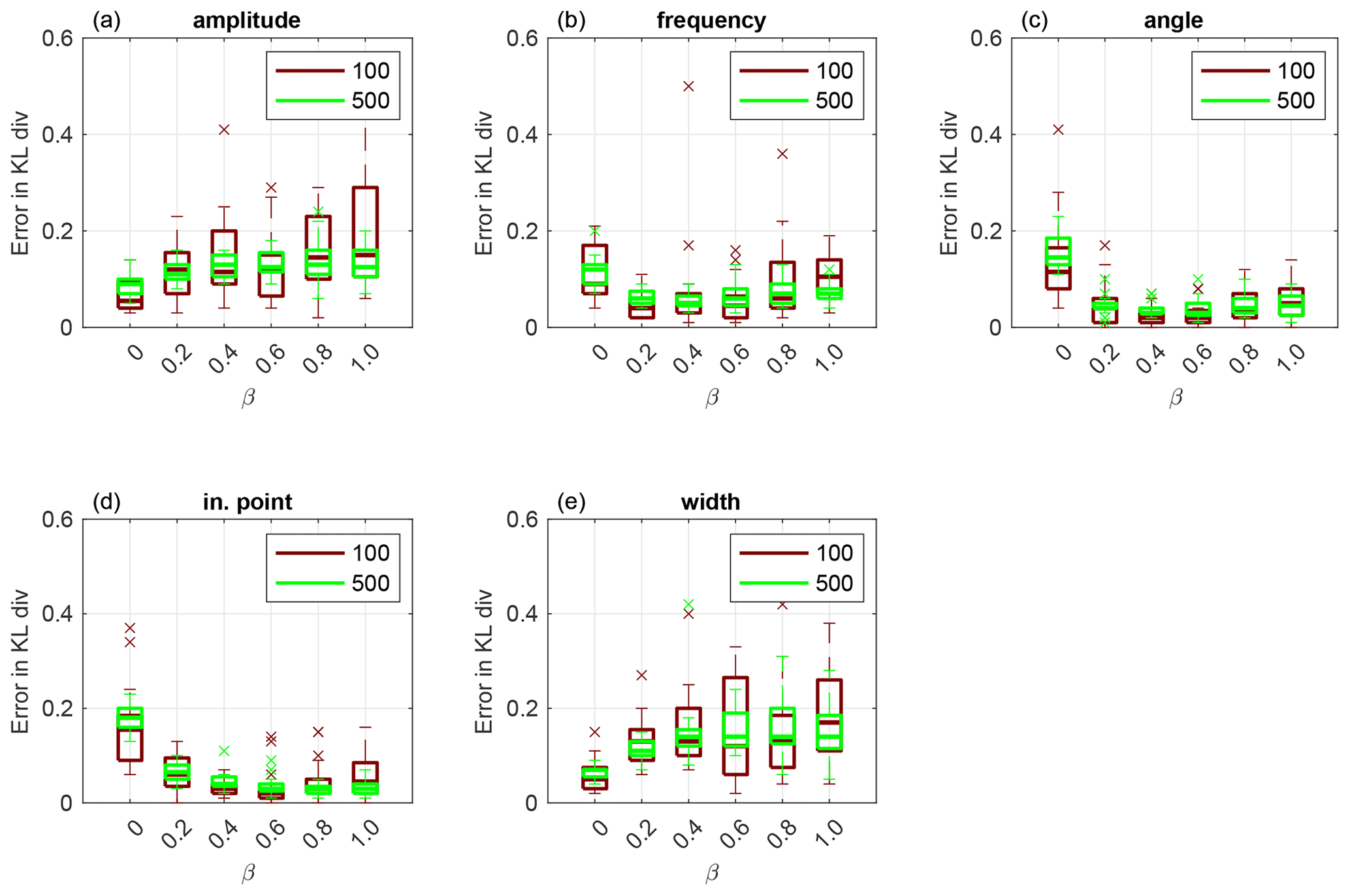
For F2, we perform numerical experiments using nine uniformly distributed observations. which are displayed in circles in Fig. 9a. First, we display results obtained using Sinkhorn approximation. In Fig. 4, we plot a box plot over 20 independent runs of KL divergence given by Eq. (19) for amplitude (a), frequency (b), angle (c), initial point (d) and width (e) that define the channel. We see that the EKI outperforms any TESPF(⋅) including the TESPF for amplitude (a) and width (e). This is due to Gaussian-like posteriors of these two geometrical parameters displayed in Fig. 6c and 6o, respectively. Due to Gaussian-like posteriors the hybrid approach decreases the RMSE compared to the TESPF: the smaller the β value, the smaller the median of the RMSE.
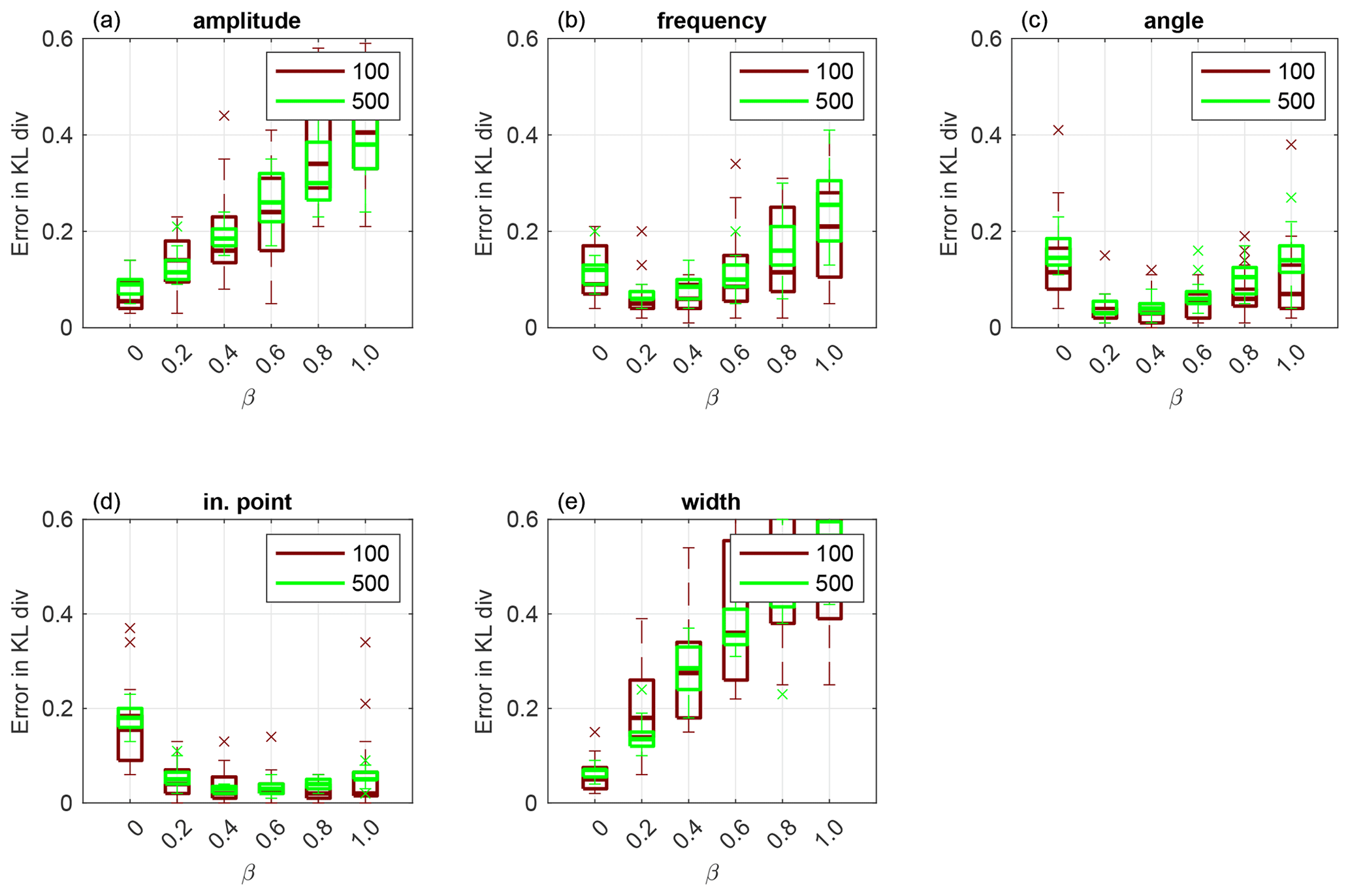
Figure 4Application to F2 parameterisation using Sinkhorn approximation. Box plot over 20 independent simulations of KL divergence for geometrical parameters: amplitude (a), frequency (b), angle (c), initial point (d) and width (e). The horizontal axis is for the hybrid parameter, where β=0 corresponds to the EKI and β=1 to TET(S)PF. Ensemble size M=100 is shown in red and M=500 in green. The central mark is the median, the edges of the box are the 25th and 75th percentiles, whiskers extend to the most extreme data points and crosses are outliers.
For frequency, angle and initial point, whose KL divergence is displayed in Fig. 4b, c and d, respectively, the behaviour of adaptive SMC is non-linear in terms of β. This is due to non Gaussian-like posteriors of these three geometrical parameters shown in Fig. 6f, i and l, respectively. Due to non Gaussian-like posteriors, the hybrid approach gives an advantage over both the TESPF and the EKI – there is a β≠0 for which the KL divergence is lowest, although it is inconsistent between geometrical parameters.
When comparing the TESPF(⋅) to the TETPF(⋅), we observe the same type of behaviour in terms of β: linear for amplitude and width, whose KL divergence is displayed in Fig. 5a and e, respectively, and non-linear for frequency, angle and initial point, whose KL divergence is displayed in Fig. 5b, c and d, respectively. However, the KL divergence is smaller when optimal transport resampling is used instead of Sinkhorn approximation.
In Fig. 6, we plot the posteriors of geometrical parameters: amplitude (a–c), frequency (d–f), angle (g–i), initial point (j–l) and width (m–o); on the left the TESPF(0.2) is shown, in the middle the TETPF(0.2) and on the right the EKI. In black is the reference, in red 20 simulations of ensemble size M=100 and in green 20 simulations of ensemble size M=500. The true parameters are shown by black crosses. We see that as the ensemble size increases, posteriors approximated by TET(S)PF converge to the reference posterior unlike the EKI.
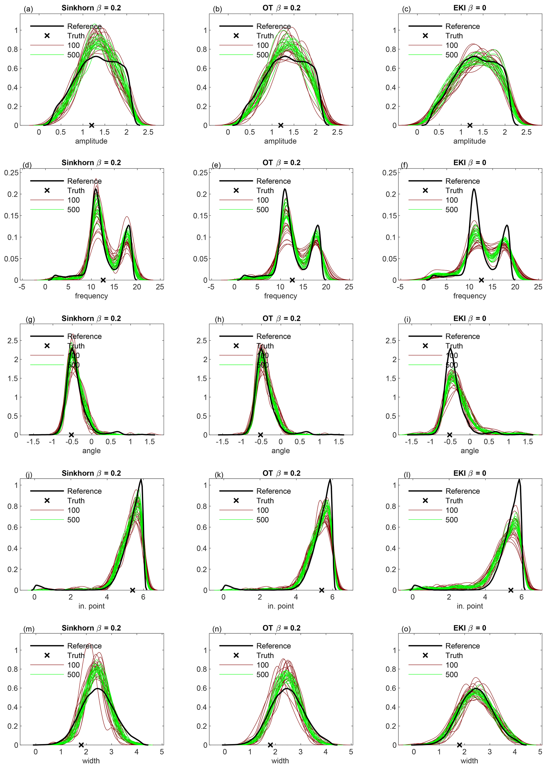
Figure 6Posteriors of geometrical parameters for F2 inference: amplitude (a–c), frequency (d–f), angle (g–i), initial point (j–l) and width (m–o). On the left is the TESPF(0.2), in the middle the TETPF(0.2) and on the right the EKI. In black is the reference, in red 20 simulations of ensemble size M=100 and in green 20 simulations of ensemble size M=500. The true parameters are shown by black crosses.
Now we investigate adaptive SMC performance for permeability estimation. First, we display results obtained using Sinkhorn approximation. The box plot shows over 20 independent simulations of the RMSE given by Eq. (18) for log permeability outside the channel in Fig. 7a and inside the channel in Fig. 7b. Even though log permeability is Gaussian-distributed, for a small ensemble size M=100, there is a β≠0 that gives the lowest RMSE both outside and inside the channel. As the ensemble size increases, the methods' performance becomes equivalent.
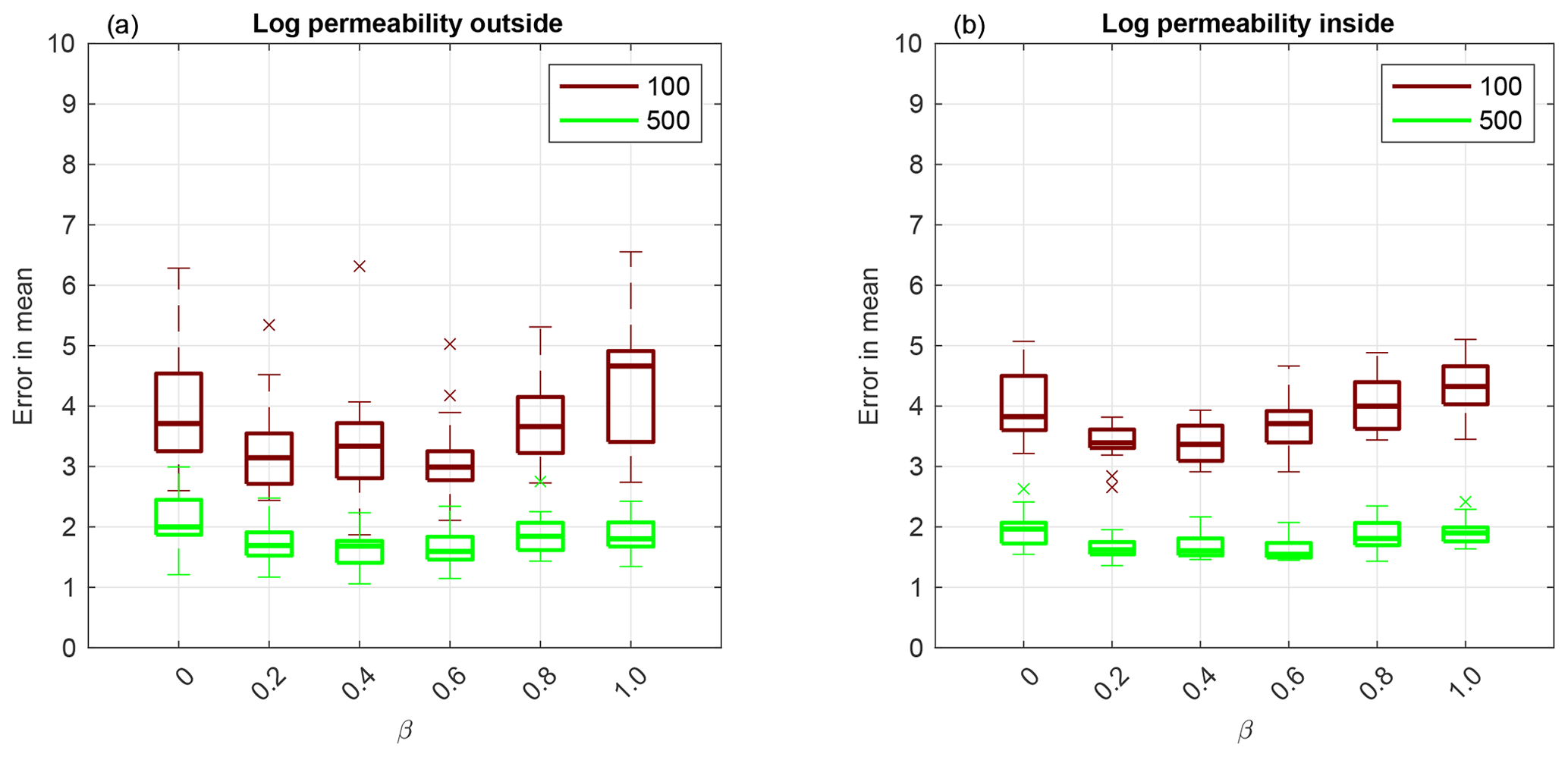
Figure 7Application to F2 parameterisation using Sinkhorn approximation. Box plot over 20 independent simulations of RMSE of mean log permeability outside the channel (a) and inside the channel (b). The horizontal axis is for the hybrid parameter, where β=0 corresponds to the EKI and β=1 to TET(S)PF. The ensemble size M=100 is shown in red and M=500 in green. The central mark is the median, the edges of the box are the 25th and 75th percentiles, whiskers extend to the most extreme data points and crosses are outliers.
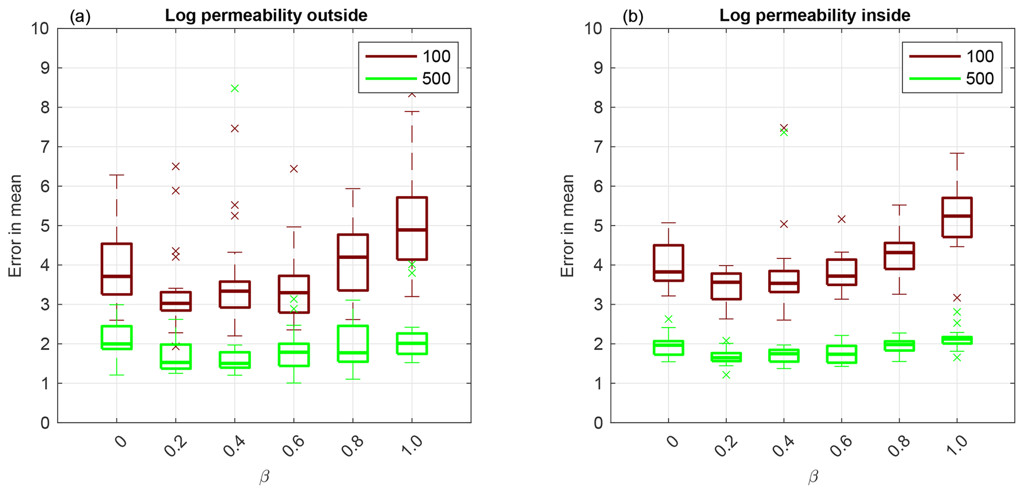
Next, we compare the TESPF(⋅) to the TETPF(⋅) for log permeability estimation outside and inside the channel, whose RMSE is displayed in Fig. 8a and b, respectively. We observe the same type of behaviour in terms of β: non-linear for a small ensemble size M=100 and equivalent for a larger ensemble size M=500. Furthermore, at a small ensemble size M=100, the TESPF outperforms the TETPF, which was also the case for F1 parameterisation (Sect. 3.4).
In Fig. 9, we show the mean field of permeability over the channelised domain for reference for the lowest error at ensemble size M=100 for the TESPF(0.2) (b), TESPF (c), EKI (d), TETPF(0.2) (e) and TETPF (f). We plot mean log permeability over the channelised domain at ensemble size M=100 and the smallest RMSE over 20 simulations in Fig. 9b–f and for the reference in Fig. 9a. We see that TESPF(0.2) does an excellent job at such a small ensemble size by estimating log permeability outside and inside the channel well, as well as parameters of the channel itself.
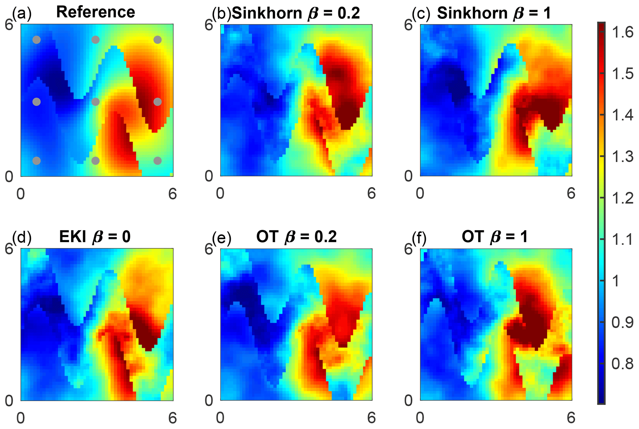
Figure 9Mean log permeability for F2 inference for the lowest error at ensemble size M=100. Observation locations are shown by circles. Reference (a), TESPF(0.2) (b), TESPF (c), EKI (d), TETPF(0.2) (e) and TETPF (f).
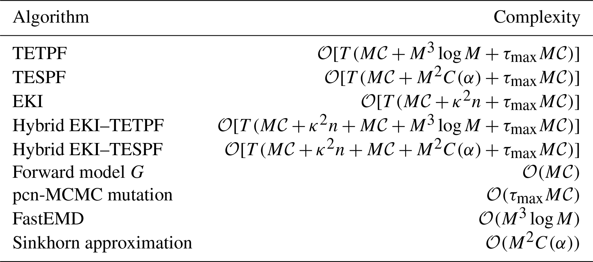
A Sinkhorn adaptation, namely the TESPF, of the previously proposed TETPF has been introduced and numerically investigated for a parameter estimation problem. The TESPF has similar accuracy results to the TETPF (see Figs. 6, 7 and 8), while it can have considerably smaller computational complexity. Specifically, the TESPF has a complexity and the TETPF (for a complete overview, see Table B1). In particular, the TESPF outperforms the EKI for non-Gaussian distributed parameters (e.g. initial point and angle in F2). This makes the proposed method a promising option for the high dimensional non-linear problems one is typically faced with in reservoir engineering. Further, to counterbalance potential robustness problems of the TETPF and its Sinkhorn adaptation, a hybrid between the EKI and the TET(S)PF is proposed and studied by means of the two configurations of the steady-state single-phase Darcy flow model. The combination of the two adaptive SMC methods with complementing properties, i.e. , is superior to the individual adaptive SMC method, i.e. β=0 or 1, for all non-Gaussian distributed parameters and performs better than the pure TETPF and the TESPF for Gaussian distributed parameters in F1. This suggests a hybrid approach has a great potential to obtain robust and highly accurate approximate solutions of non-linear high dimensional Bayesian inference problems. Note that we have considered a synthetic case, where the truth is available, and thus chose β in terms of accuracy of an estimate. However, in a realistic application, the truth is not provided. In the context of state estimation with an underlying dynamical system, it has been suggested to adaptively change the hybrid parameter with respect to the effective sample size. As the tempering scheme is already changed according to the effective sample size, this ansatz would require the interplay between the two tuning variables to be defined. An ad hoc choice for β could be 0.2 or 0.3. This is motivated by the fact that the particle filter is too unstable in high dimensions, and it is therefore sensible to use a tuning parameter prioritising the EKI. The ad hoc choice is supported by the numerical results in Sect. 3 and in Acevedo et al. (2017) and de Wiljes et al. (2020) in the context of state estimation.
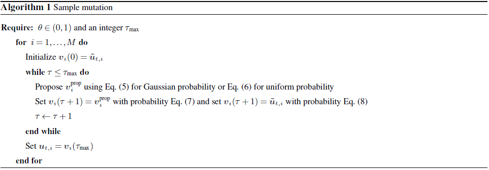
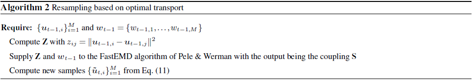
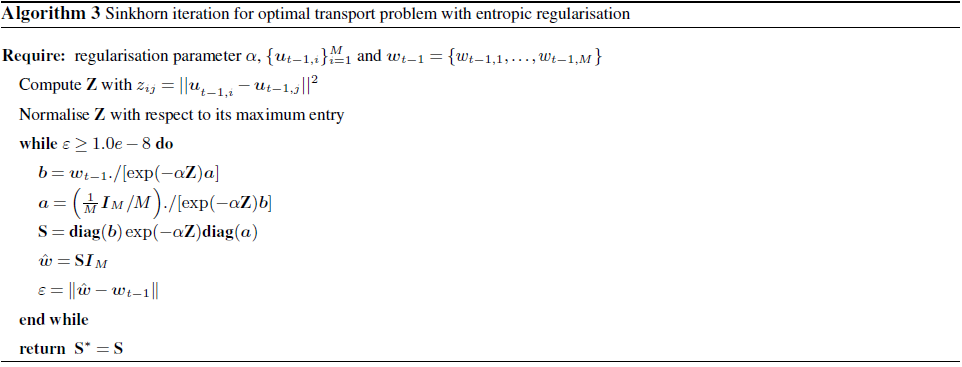
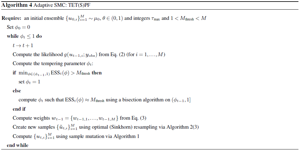
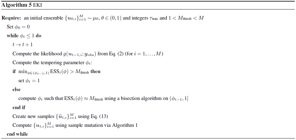
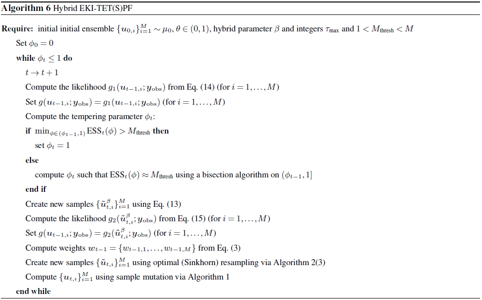
Table B1The table provides an overview of the computational complexity of all the algorithms considered in the paper.
Data and MATLAB codes for generating the plots are available at https://doi.org/10.4121/12987719 (Ruchi et al., 2021).
SR, SD and JdW designed the research. SD ran the numerical experiments. SR, SD and JdW analysed the results and wrote the paper.
The authors declare that they have no conflict of interest.
The research of Jana de Wiljes and Sangeetika Ruchi have been partially funded by the Deutsche Forschungsgemeinschaft (DFG) SFB 1294/1 – 318763901. Further, Jana de Wiljes has been supported by Simons CRM Scholar-in-Residence Program and ERC Advanced Grant ACRCC (grant no. 339390). Sangeetika Ruchi has been supported by the research programme Shell-NWO/FOM Computational Sciences for Energy Research (CSER), project no. 14CSER007, which is partly financed by the Netherlands Organization for Scientific Research (NWO).
This research has been supported by the Deutsche Forschungsgemeinschaft (grant no. SFB1294/1 – 318763901), the European Research Council (Advanced Grant ACRCC (grant no. 375 339390)), the Nederlandse Organisatie voor Wetenschappelijk Onderzoek, Stichting voor de Technische Wetenschappen (grant no. Shell-NWO/FOM Computational Sciences for Energy Research (CSER), project no. 14CSER007) and the Simons Foundation (CRM Scholar-in-Residence Program grant).
This paper was edited by Olivier Talagrand and reviewed by Femke Vossepoel and Marc Bocquet.
Acevedo, W., de Wiljes, J., and Reich, S.: Second-order Accurate Ensemble Transform Particle Filters, SIAM J. Sci. Comput., 39, A1834–A1850, 2017. a, b
Agapiou, S., Papaspiliopoulos, O., Sanz-Alonso, D., and Stuart, A. M.: Importance sampling: computational complexity and intrinsic dimension, Stat. Sci., 32, 405–431, https://doi.org/10.1214/17-STS611, 2017. a
Bardsley, J., Solonen, A., Haario, H., and Laine, M.: Randomize-then-optimize: A method for sampling from posterior distributions in nonlinear inverse problems, SIAM J. Sci. Comput., 36, A1895–A1910, 2014. a, b
Beskos, A., Crisan, D., and Jasra, A.: On the stability of sequential Monte Carlo methods in high dimensions, Ann. Appl. Probab., 24, 1396–1445, https://doi.org/10.1214/13-AAP951, 2014. a
Beskos, A., Jasra, A., Muzaffer, E. A., and Stuart, A. M.: Sequential Monte Carlo methods for Bayesian elliptic inverse problems, Stat. Comput., 25, 727–737, https://doi.org/10.1007/s11222-015-9556-7, 2015. a
Blömker, D., Schillings, C., Wacker, P., and Weissmann, S.: Well posedness and convergence analysis of the ensemble Kalman inversion, Inverse Probl., 35, 085007, https://doi.org/10.1088/1361-6420/ab149c, 2019. a, b
Chen, Y. and Oliver, D.: Ensemble randomized maximum likelihood method as an iterative ensemble smoother, Math. Geosci., 44, 1–26, 2012. a
Chustagulprom, N., Reich, S., and Reinhardt, M.: A Hybrid Ensemble Transform Particle Filter for Nonlinear and Spatially Extended Dynamical Systems, SIAM/ASA Journal on Uncertainty Quantification, 4, 592–608, https://doi.org/10.1137/15M1040967, 2016. a, b, c
Cotter, S., Roberts, G., Stuart, A., and White, D.: MCMC methods for functions: modifying old algorithms to make them faster, Stat. Sci., 28, 424–446, 2013. a, b, c, d
Cuturi, M.: Sinkhorn Distances: Lightspeed Computation of Optimal Transport, in: Advances in Neural Information Processing Systems 26, edited by: Burges, C. J. C., Bottou, L., Welling, M., Ghahramani, Z., and Weinberger, K. Q., available at: http://papers.nips.cc/paper/4927-sinkhorn-distances-lightspeed-computation-of-optimal-transport.pdf (last access: 29 December 2020), Curran Associates, Inc., 2292–2300, 2013. a, b
Dashti, M. and Stuart, A. M.: The Bayesian Approach to Inverse Problems, Springer International Publishing, Cham, 311–428, https://doi.org/10.1007/978-3-319-12385-1_7, 2017. a
Del Moral, P., Doucet, A., and Jasra, A.: Sequential Monte Carlo samplers, J. Roy. Stat. Soc. B, 68, 411–436, https://doi.org/10.1111/j.1467-9868.2006.00553.x, 2006. a, b
de Wiljes, J., Pathiraja, S., and Reich, S.: Ensemble Transform Algorithms for Nonlinear Smoothing Problems, SIAM J. Sci. Comput., 42, A87–A114, 2020. a, b
Emerick, A. and Reynolds, A.: Ensemble smoother with multiple data assimilation, Comput. Geosci., 55, 3–15, 2013. a
Ernst, O. G., Sprungk, B., and Starkloff, H.-J.: Analysis of the Ensemble and Polynomial Chaos Kalman Filters in Bayesian Inverse Problems, SIAM/ASA Journal on Uncertainty Quantification, 3, 823–851, https://doi.org/10.1137/140981319, 2015. a
Evensen, G.: Analysis of iterative ensemble smoothers for solving inverse problems, Computat. Geosci., 22, 885–908, https://doi.org/10.1002/qj.2236, 2018. a
Frei, M. and Künsch, H. R.: Bridging the ensemble Kalman and particle filters, Biometrika, 100, 781–800, https://doi.org/10.1093/biomet/ast020, 2013. a, b
Hairer, M., Stuart, A., and Vollmer, S.: Spectral gaps for a Metropolis–Hastings algorithm in infinite dimensions, Ann. Appl. Probab., 24, 2455–2490, 2014. a
Hoang, V. H., Schwab, C., and Stuart, A. M.: Complexity analysis of accelerated MCMC methods for Bayesian inversion, Inverse Probl., 29, 085010, https://doi.org/10.1088/0266-5611/29/8/085010, 2013. a
Houtekamer, P. L. and Zhang, F.: Review of the Ensemble Kalman Filter for Atmospheric Data Assimilation, Mon. Weather Rev., 144, 4489–4532, https://doi.org/10.1175/MWR-D-15-0440.1, 2016. a
Iglesias, M., Park, M., and Tretyakov, M.: Bayesian inversion in resin transfer molding, Inverse Probl., 34, 105002, https://doi.org/10.1088/1361-6420/aad1cc, 2018. a, b, c
Iglesias, M. A.: A regularizing iterative ensemble Kalman method for PDE-constrained inverse problems, Inverse Probl., 32, 025002, https://doi.org/10.1088/0266-5611/32/2/025002, 2016. a
Iglesias, M. A., Lin, K., and Stuart, A. M.: Well-posed Bayesian geometric inverse problems arising in subsurface flow, Inverse Probl., 30, 114001, https://doi.org/10.1088/0266-5611/30/11/114001, 2014. a, b, c, d
Kantorovich, L. V.: On the translocation of masses, Dokl. Akad. Nauk. USSR (NS), 37, 199–201, 1942. a
Le Gland, F., Monbet, V., and Tran, V.-D.: Large sample asymptotics for the ensemble Kalman Filter, Research Report, R-7014, INRIA, available at: https://hal.inria.fr/inria-00409060/file/RR-7014.pdf (last access: 14 November 2020), 2009. a
Liu, Y., Haussaire, J., Bocquet, M., Roustan, Y., Saunier, O., and Mathieu, A.: Uncertainty quantification of pollutant source retrieval: comparison of Bayesian methods with application to the Chernobyl and Fukushima-Daiichi accidental releases of radionuclides, Q. J. Roy. Meteor. Soc., 143, 2886–2901, 2017. a
Lorentzen, R. J., Bhakta, T., Grana, D., Luo, X., Valestrand, R., and Nævdal, G.: Simultaneous assimilation of production and seismic data: application to the Norne field, Computat. Geosci., 24, 907–920, https://doi.org/10.1007/s10596-019-09900-0, 2020. a
Matérn, B.: Spatial Variation, Lecture Notes in Statistics, No. 36, Springer-Verlag New York, USA, https://doi.org/10.1007/978-1-4615-7892-5, 1986. a
Monge, G.: Mémoire sur la théorie des déblais et des remblais, Histoire de l'Académie Royale des Sciences de Paris, avec les Mémoires de Mathématique et de Physique pour la même année, 666–704, 1781. a
Neal, R. M.: Annealed importance sampling, Stat. Comput., 11, 125–139, 2001. a, b
Oliver, D., He, N., and Reynolds, A.: Conditioning permeability fields to pressure data, ECMOR V-5th European Conference on the Mathematics of Oil Recovery, Leoben, Austria, 3–6 September 1996, pp. 259–269, 1996. a, b
Pele, O. and Werman, M.: Fast and robust earth mover's distances, in: Computer vision, 2009 IEEE 12th international conference on Computer Vision, Kyoto, Japan, 29 September–2 October 2009, pp. 460–467, IEEE, https://doi.org/10.1109/ICCV.2009.5459199, 2009. a
Peyré, G. and Cuturi, M.: Computational Optimal Transport: With Applications to Data Science, in: Foundations and Trends(r) in Machine Learning, 11, 355–607, https://doi.org/10.1561/2200000073, 2019. a
Reich, S.: A nonparametric ensemble transform method for Bayesian inference, SIAM Journal on Scientific Computing, 35, A2013–A2024, 2013. a, b, c, d
Robert, C. and Casella, G.: Monte Carlo Statistical Methods, 2nd Edn., Springer, New York, 2004. a
Roberts, G. O. and Rosenthal, J. S.: Optimal scaling for various Metropolis-Hastings algorithms, Stat. Sci., 16, 351–367, https://doi.org/10.1214/ss/1015346320, 2001. a
Rosenthal, J. S.: Markov Chain Monte Carlo Algorithms: Theory and Practice, in: Monte Carlo and Quasi-Monte Carlo Methods 2008, edited by: L'Ecuyer, P. and Owen, A. B., Springer Berlin Heidelberg, 157–169, https://doi.org/10.1007/978-3-642-04107-5, 2009. a
Ruchi, S., Dubinkina, S., and Iglesias, M. A.: Transform-based particle filtering for elliptic Bayesian inverse problems, Inverse Probl., 35, 115005, https://doi.org/10.1088/1361-6420/ab30f3, 2019. a, b, c, d, e
Ruchi, S., Dubinkina, S., and de Wiljes, J.: Data underlying the paper: Application of ensemble transform data assimilation methods for parameter estimation in nonlinear problems, 4TU, Centre for Research Data, Dataset, https://doi.org/10.4121/12987719, 2021. a
Santitissadeekorn, N. and Jones, C.: Two-Stage Filtering for Joint State-Parameter Estimation, Mon. Weather Rev., 143, 2028–2042, https://doi.org/10.1175/MWR-D-14-00176.1, 2015. a
Sinkhorn, R.: Diagonal equivalence to matrices with prescribed row and column sums, Am. Math. Mon., 74, 402–405, 1967. a
Stordal, A., Karlsen, H. A., Nævdal, G., Skaug, H., and Vallès, B.: Bridging the ensemble Kalman filter and particle filters: the adaptive Gaussian mixture filter, Computat. Geosci., 15, 293–305, https://doi.org/10.1007/s10596-010-9207-1, 2011. a, b
Stuart, A. M.: Inverse problems: a Bayesian perspective, Acta Numer., 19, 451–559, 2010. a
Vergé, C., Dubarry, C., Del Moral, P., and Moulines, E.: On parallel implementation of sequential Monte Carlo methods: the island particle model, Stat. Comput., 25, 243–260, https://doi.org/10.1007/s11222-013-9429-x, 2015. a
Zovi, F., Camporese, M., Hendricks Franssen, H.-J., Huisman, J. A., and Salandin, P.: Identification of high-permeability subsurface structures with multiple point geostatistics and normal score ensemble Kalman filter, J. Hydrol., 548, 208–224, https://doi.org/10.1016/j.jhydrol.2017.02.056, 2017. a
Note that the terminology is also used in the context of data assimilation filters combining variational and sequential approaches.