MESMER-RCM: a probabilistic climate emulator for regional warming projections

Regional Climate Model (RCM) emulators enable rapid and computationally efficient RCM projections given Global Climate Model (GCM) inputs, complementing dynamical downscaling by approximating physical representations with statistical models. However, while existing RCM emulators perform well in deterministic emulations, they do not sample internal RCM variability and remain computationally expensive. Here, we present MESMER-RCM, a probabilistic RCM emulator designed for spatially resolved annual 2 m temperature. MESMER-RCM is a generative model that enables both data-efficient learning and interpretability. It can generate large ensembles of synthetic, yet physically plausible, RCM realizations, capturing the internal RCM variability at a fraction of the computational cost. This work offers a fast and reliable RCM emulation framework, supporting finer-scale what-if analyses of regional climate responses and informing local adaptation and mitigation strategies.

1 Introduction

Warming at regional scales is a critical aspect of climate change as humans and natural systems are affected by local temperatures and not the global mean. Warming patterns vary spatially with geographical features, with amplification in urbanized and deforested regions (IPCC, 2023), as well as in mountainous areas (Mountain Research Initiative EDW Working Group, 2015). These heterogeneous warming patterns necessitate finer-scale climate projections, often achieved using Regional Climate Models (RCMs) downscaling Global Climate Model (GCM) simulations (Soares et al., 2022; Careto et al., 2022; Jacob et al., 2020; Roberts et al., 2019). However, these high-resolution simulations are computationally expensive and the need to explore uncertainty within multiple models and scenario pathways significantly increases computational demands. In addition, representing internal climate variability requires large initial-condition ensembles (Eyring et al., 2024; Schneider et al., 2023; Giorgi, 2019; Hawkins and Sutton, 2009), further escalating the overall cost.

Recent advancements in climate emulators address these challenges by simplifying model complexity, thus enabling rapid climate projections under various scenario pathways. Among these, RCM emulators have gained attention as efficient surrogates for RCMs, providing insights into regional climate projections. While both RCM emulators and statistical downscaling methods aim to bridge the gap between coarse-resolution GCM outputs and fine-scale regional climate information, they differ in their setup and objectives. RCM emulators are trained on GCM-RCM model chain simulations to reproduce RCM outputs, whereas statistical downscaling methods rely on empirical relationships derived from observational data to establish connections between large-scale and local-scale climate variables. Thus, RCM emulators and statistical downscaling methods can inform each other. Leveraging both deep neural networks (Doury et al., 2023, 2024; Van Der Meer et al., 2023; Baño-Medina et al., 2022; Passarella et al., 2022) and classical statistic approaches (Hobeichi et al., 2023; Boé and Mass, 2022), recent advancements in RCM emulators have achieved remarkable accuracy and efficiency. Moreover, efforts have been made to enhance interpretability of RCM emulators (González-Abad et al., 2023; Baño-Medina et al., 2022) and to evaluate transferability across emission scenarios, initial-condition ensembles, and GCMs (Hernanz et al., 2024, 2022; Bano-Medina et al., 2023).

Despite these advancements, current RCM emulators focus primarily on deterministic prediction and do not fully account for the internal RCM variability, which is essential for useful regional climate projections. Recently, deep learning-based generative models have shown promising performance in probabilistic ensemble downscaling by enabling realistic sampling of internal variability (Lopez-Gomez et al., 2024; Watt and Mansfield, 2024; Ling et al., 2024; Bischoff and Deck, 2024; Tomasi et al., 2024; Mardani et al., 2024; Wan et al., 2023). However, the inherent complexity of these models poses challenges for interpretability and requires significant computational resources during training and inference. Furthermore, these highly flexible models may fail to achieve optimal performance due to the currently limited sample size of GCM-RCM simulations that are available for training. To address these gaps, we present MESMER-RCM, a probabilistic ensemble RCM emulator designed for spatially-resolved annual 2 m temperature projections. MESMER-RCM is a generative model that achieves both interpretability and data-efficient learning. This study focuses on an RCM emulator tailored for the Europe (EURO-CORDEX, Gutowski et al., 2016), with potential applicability to other regions. MESMER-RCM can be integrated with GCM emulators such as MESMER (Beusch et al., 2020b), providing a foundation for building an robust GCM–RCM emulator chain for future applications.

2 Data

MESMER-RCM is trained and tested using simulations from the EURO-CORDEX-CMIP5 experiment (Gutowski et al., 2016; Taylor et al., 2012). EURO-CORDEX-CMIP5 provides RCM simulations forced by the output from a specific GCM, named a GCM-RCM model chain. We use RCM simulations with a spatial resolutions of 0.44° and re-grid GCM data to a common resolution of 2.5°. The dataset aligns with the one used in the Fischer et al. (2018). This study focuses on annual mean 2 m air temperature, for the period 1971 to 2099, and land grid points in the RCM domain (−25 to 45° E, 26 to 72° N). Each RCM simulation consists of 129 years of data and land 5929 grid points. The dataset contains 42 simulations (Table S1 in the Supplement), from five RCMs and nine GCMs under the Representative Concentration Pathways (RCP) 2.6, 4.5, and 8.5 scenario pathways (Meinshausen et al., 2011).

The simulation matrix for GCM-RCM combinations in EURO-CORDEX is sparse, with SMHI-RCA4 dominating the available model chains (Table S1). Additionally, not all model chains provide all scenarios and there are only few which contributed initial-condition ensembles. These limitations and their implications for the methodology are discussed in detail in Sect. 5.3. Nonetheless, the dataset provides a diverse set of GCM-RCM combinations under key scenario pathways, making it suitable to evaluate the performance of MESMER-RCM in emulating different GCM-RCM model chains and exploring various scenario pathways.

3 MESMER-RCM: A framework for regional climate model emulation

3.1 MESMER-RCM structure

MESMER-RCM explicitly models the annual mean temperature at an RCM grid point i and time step t as a linear combination of the RCM response to the driving GCM and a residual climate variability term:

$$\begin{array}{}\text{(1)}& T_{i,t}^{\mathrm{RCM}}=f(T_{s,t}^{\mathrm{GCM}}{)}_{i,t}+{\mathit{\eta }}_{i,t}^{\mathrm{RCM}}\end{array}$$

where $f(T_{s,t}^{\mathrm{GCM}}{)}_{i,t}$ denotes the deterministic response of the RCM at grid point i (for all i) to the GCM temperature at grid point s, and ${\mathit{\eta }}_{i,t}^{\mathrm{RCM}}$ represents the residual variability. The deterministic response term captures the systematic relationship between GCM and RCM simulations, while the residual variability term approximates the additional internal variability implied by the RCM as a stochastic process. The schematic overview of MESMER-RCM is shown in Fig. 1.

Figure 1 Schematic overview of the MESMER-RCM methodology, which statistically emulates regional climate model (RCM) outputs from global climate model (GCM) inputs. The upper box illustrates the mathematical formulation and structure of MESMER-RCM, showing how RCM temperatures are represented as statistical functions of GCM temperatures through a deterministic component and a stochastic residual. The lower-left box explains how the training and testing data sets are split. An example for a model chain with three simulation pairs is shown in the table: for each simulation pair i used for training (Train i), the remaining two simulation pairs are used for testing (Test i−1 and Test i−2), resulting in six training–testing experiments in total. The total number of training–testing experiments depends on the available simulation pairs, as indicated by the permutation formula in the box. The lower-right box outlines the training procedure of MESMER-RCM, which follows a modular training strategy. The steps related to the prior P are shown in gray text, as they need to be performed before Step 4 but not necessarily after Steps 1–3.

3.2 Deterministic response module

We use Lasso multiple linear regression (Lasso MLR) for mapping the deterministic RCM temperature response of GCM in Eq. (1):

$$\begin{array}{}\text{(2)}& f(T_{s,t}^{\mathrm{GCM}}{)}_{i,t}=a_i^{\mathrm{int}}+\sum _{s\in N_k\left(i\right)}{a}_{i,s}{T}_{s,t}^{\mathrm{GCM}}\end{array}$$

The predictors are the 2 m temperature at the k GCM grid points closest to the RCM grid point i (i.e., s∈N_k(i)). Here, a_i,s represents the scaling coefficients that determine the influence of GCM grid points on RCM grid point i, while $a_i^{\mathrm{int}}$ captures the local intercept. The scaling coefficients a_i,s for corresponding GCM predictors are optimized by minimizing a lasso loss that combines the least squares term and an L1 normalization term, $\mathit{\lambda }\cdot {\sum }_{s=\mathrm{1}}^k\left|a_{i,s}\right|$ (James et al., 2013). The L1 regularization adaptively selects the most relevant GCM grid points for predicting RCM temperature while shrinking the scaling coefficients of less relevant contributions towards zero. In this study, we use the nine nearest GCM grid points surrounding each RCM grid point as predictors (k = 9). Specifically, we first identify the GCM grid point closest to the RCM grid point based on Euclidean distance, and then select the surrounding eight neighbors to form a 3×3 local grid that captures the GCM information around the RCM location.

3.3 Residual variability module

The residual variability term, ${\mathit{\eta }}_{i,t}^{\mathrm{RCM},\mathrm{res}}$, is assumed to follow a multivariate Gaussian distribution (see Fig. S1 in the Supplement for the results of Shapiro–Wilk test for normality), ${\mathit{\eta }}_{i,t}^{\mathrm{RCM},\mathrm{res}}\sim \mathcal{N}(\mathrm{0},{\mathbf{\Sigma }}_{\mathrm{RCM}}^{\mathrm{res}})$, where ${\mathbf{\Sigma }}_{\mathrm{RCM}}^{\mathrm{res}}$ denotes the spatial covariance matrix across all considered RCM grid points, that is estimated from the residuals after subtracting the deterministic response. However, since each RCM simulation includes far more grid points than sample years, the sample covariance matrix of the residuals ${\widehat{\mathbf{\Sigma }}}_{\mathrm{RCM}}^{\mathrm{res}}$ becomes rank-deficient and needs to be regularized to improve the accuracy and stability of the estimate (Stein, 1956; Ledoit and Wolf, 2003; Pourahmadi, 2011). This is often achieved by shrinking the sample covariance matrix $\widehat{\mathbf{S}}$ to a target covariance matrix T that encapsulates prior knowledge on the dependence structure of the underlying process such that

$$\begin{array}{}\text{(3)}& S=\mathit{\alpha }\mathbf{T}+(\mathrm{1}-\mathit{\alpha })\widehat{\mathbf{S}}\end{array}$$

where α is the shrinkage parameter. Typical shrinkage targets are diagonal matrices such as the unit matrix since they are full rank. However, these assume independence for non-diagonal entries of the covariance matrix, which is physically not consistent with climate variability that is strongly correlated in space.

To address this limitation, we propose to leverage the full ensemble of RCM simulations to construct a data-driven prior, P, for T. The prior P is estimated by first concatenating the residuals of all RCM simulations, except those used for training and testing, and subsequent computations of an sample covariance matrix. Due to the increased sample size, P is nearly full rank and incorporates knowledge on the covariance structure derived from the available RCM simulations. However, P remains rank deficient and hence needs and is shrunken to $\mathbf{\Lambda }=\mathrm{diag}\left({\widehat{\mathbf{\Sigma }}}_{\mathrm{RCM}}^{\mathrm{res}}\right)$ which incorporates prior knowledge that sample variances typically have lower estimation errors than the covariances. The resulting shrinkage estimator can thus be written as

$$\begin{array}{}\text{(4)}& \begin{array}{rl}{\mathbf{\Sigma }}_{\mathrm{RCM}}^{\mathrm{res}}(\mathit{\alpha },\mathit{\beta })& =\mathit{\alpha }\cdot \left[\right(\mathrm{1}-\mathit{\beta })\cdot \mathbf{P}+\mathit{\beta }\cdot \mathbf{\Lambda }]\\ & +(\mathrm{1}-\mathit{\alpha })\cdot {\widehat{\mathbf{\Sigma }}}_{\mathrm{RCM}}^{\mathrm{res}}\end{array}\end{array}$$

4 Applying MESMER-RCM

4.1 Training and testing data sets

To train and test MESMER-RCM we use RCM simulations provided by the EURO-CORDEX ensemble and its driving GCM simulation from the CMIP5 ensemble (hereafter termed a simulation pair). We generally use one simulation pair for training and testing, respectively, except for some sensitivity test where we use more than one pair for training (Sect. 4.4). We train and test MESMER-RCM for each GCM-RCM model chain individually. The difference between training and testing sample thus comes from different forcing scenarios and/or initial conditions. We design the training–testing experiments by exhaustively considering all possible training–testing permutations of the available simulation pairs (Fig. 1). For instance, if there are two available simulation pairs in a model chain that differ in their scenarios, RCP4.5 and RCP8.5, we train MESMER-RCM on RCP4.5 and test on RCP8.5, and vice versa. The number of training–testing experiments for individual model chain can be calculated using the number of permutations, $P(n_{\mathrm{train}}+n_{\mathrm{test}},n_{\mathrm{sim}})=\frac{(n_{\mathrm{train}}+n_{\mathrm{test}})\mathrm{!}}{(n_{\mathrm{train}}+n_{\mathrm{test}}-n_{\mathrm{sim}})\mathrm{!}}$, where n_sim is the available number of simulation pairs, n_train and n_test are the number of simulation pairs used for training and testing, respectively.

In our framework, the prior P is decoupled from the training–testing design. For each training–testing experiment, P is constructed from the residuals of all RCM simulations other than those selected for training and testing, and is then kept fixed and identical across both phases within the experiment.

4.2 Modular training and emulation

MESMER-RCM follows a modular training approach, where the deterministic response and the residual variability module are learned separately. Firstly, we calibrate $a_i^{\mathrm{int}}$ and a_i,s by minimizing the lasso loss of Eq. (2) using coordinate descent. The lasso coefficients λ_s are determined through a cross-validation exercise based on minimum mean absolute error (James et al., 2013). The search range for λ_s spans from 10⁻⁴ to 10¹ with half-order-of-magnitude steps. In this study, we keep λ_s the same across all grid points as the the optimal lasso coefficients exhibit spatial smoothness.

Secondly, we derive the residual ${\mathit{\eta }}_{i,t}^{\mathrm{RCM}}$ as the difference between the RCM temperature $T_{s,t}^{\mathrm{RCM}}$ and the deterministic response $f\left(T_{s,t}^{\mathrm{GCM}}\right)$, the latter projected from the calibrated coefficients $a_i^{\mathrm{int}}$ and a_i,s using the GCM reference temperature $T_{s,t}^{\mathrm{GCM}}$. We then jointly calibrate the shrinkage coefficients α and β in Eq. (4) by maximizing the Gaussian log-likelihood through a grid search with 5-fold cross-validation. The search range for α is 0.1 to 1.0 in increments of 0.1, and for β it is 10⁻⁴ to 10¹ with half-order-of-magnitude steps. The prior P was constructed ahead and is kept fixed during the cross-validation experiments, while Λ and ${\widehat{\mathbf{\Sigma }}}_{\mathrm{RCM}}^{\mathrm{res}}$ are re-estimated in each training fold. The log-likelihood is evaluated on the testing folds by measuring the distributional fit between the held-out data and $\mathcal{N}(\mathrm{0},{\mathbf{\Sigma }}_{\mathrm{RCM}}^{\mathrm{res}}(\mathit{\alpha },\mathit{\beta }\left)\right)$.

To generate an ensemble of M RCM emulations, we first apply the deterministic response module (Eq. 2), replicate its output M times, and then add spatially correlated residuals drawn from the residual variability module (Eq. 4) to each copy.

4.3 Evaluation of MESMER-RCM performance

We first evaluate the reliability of MESMER-RCM as a ensemble prediction system using a rank histogram (Wilks, 2006, 2019; Weigel et al., 2008; Jolliffe, 2012). Reliability here refers to the calibration of MESMER-RCM, and whether the RCM emulation spread well captures the RCM reference, and is hence a suitable metric to evaluate our probabilistic emulator. The idea of a rank histogram is as follow: for each ensemble prediction (or here emulation) consisting of M ensemble members, the verifying reference is combined with the ensemble members to form a vector of M+1 values. The reference is ranked within this vector, where rank 1 is assigned to the smallest, and rank M+1 to the largest value within the ensemble. If the reference is statistically indistinguishable from the ensemble predictions, then each rank is equally likely to occur. In such cases, the rank histogram will be flat, apart from small fluctuations caused by sampling variability. Deviations from flatness in the rank histogram indicate MESMER-RCM miscalibration, arising either from bias in the mean due to the deterministic response module or from bias in the variance due to the residual variability module. We test the rank histogram flatness at the grid-point level using the χ² statistic (Wilks, 2019), and compute the χ² test pass rate defined as the percentage of grid points for which the null hypothesis of flatness is not rejected, for each training–testing experiment.

Noting that the rank histogram mostly focus on the correct specification of variance (Hamill, 2001), we complement it with an evaluation of the Gaussian likelihood function as it can take into account the full covariance structure. The likelihood function measures the probability of the RCM reference for each year given the emulated distribution $\mathcal{N}\left(f\right(T_{s,t}^{\mathrm{GCM}}),{\mathbf{\Sigma }}_{\mathrm{RCM}}^{\mathrm{res}})$, an analogy of emulator's ability to emulate the distribution of the RCM reference. We then compare MESMER-RCM with benchmarks using the likelihood function. We propose benchmark methods using the similar structure as MESMER-RCM. Our benchmark for the deterministic response module is a simple linear regression, where the predictor is only the nearest GCM grid point temperature (k = 1 in Eq. 2), while we use the Ledoit-Wolf estimator (Ledoit and Wolf, 2004) as benchmark for the residual variability module. The Ledoit-Wolf estimator is commonly used to estimate the covariance matrix in high-dimensional settings, and has wide application in finance and machine learning. Additionally, we propose a naive benchmark for residual variability module using the sample variance matrix Λ that assumes spatial independence as reference. Since Λ is full rank, innovations can be directly drawn from a multivariate Gaussian 𝒩(0,Λ) without regularization.

4.4 Sensitivity to Training Configurations

Given the sparsity of GCM–RCM simulations in the EURO-CORDEX ensemble (Table S1), it is crucial to evaluate how model performance varies with different training sample size. In this study, we conduct three sensitivity experiments that use different samples to train the deterministic response module, the prior P in the residual variability module, and both, respectively.

1. To assess the robustness of the deterministic response module (Eq. 2), we train it using concatenated GCM–RCM simulation pairs from all available ensemble members, except the pair currently used for testing (i.e., $n_{\mathrm{train}}=n_{\mathrm{sim}}-n_{\mathrm{test}}$, with n_test = 1).

2. The sample–consistency trade-off in the residual variability module (Eq. 4) is evaluated by constructing the prior P from a reduced set of concatenated RCM residuals, selected for their higher physical consistency with the training set.

3. Combined approach: Applying both (1) and (2) simultaneously. Performance differences are evaluated using the χ² test pass rate.

5 Results

5.1 Calibration of MESMER-RCM

The deterministic response module is calibrated for each grid-cell individually but working with the same Lasso coefficient (λ = 0.005) across all grid-cells and model chains. The common lasso coefficient is chosen based on a cross-validation exercise which showed that the optimized Lasso coefficients exhibit spatial smoothness, with the European land mean stabilizing around 0.005 across all simulations (Fig. S2 in the Supplement). A summary of the coefficients of the deterministic response module alongside some insights to their spatial variability is provided in the Supplement (Figs. S3, S4). The sum of scaling coefficients (${\sum }_{s\in N_k\left(i\right)}{a}_{i,s}$) shows higher values in mountainous regions and high-latitude areas, highlighting the capacity of deterministic response module to capture elevation-dependent warming and polar amplification, respectively. The scaling coefficients indicate that RCM grid points in the Swiss Alps warm faster than its northwest and southeast GCM counterparts. This pattern may be related to the north/south foehn effect over the Alpine region (Chow et al., 2013).

The shrinkage coefficients (α, β) in the residual variability module is calibrated for each model chain. The resulting log-likelihood field associated with α and β are consistent across all model chains, where the optimum β is around 10⁻² for stabilizing ${\widehat{\mathbf{\Sigma }}}_{\mathrm{RCM}}^{\mathrm{res}}$ and α is around 10⁻¹ for effectively borrowing prior information from P. An example of such a log-likelihood field is provided in the Supplement (Fig. S5)

5.2 Example of ensemble RCM emulations

Figure 2 presents an example of RCM emulations for an GCM-RCM model chain (RCM: SMHI-RCA4, GCM: CanESM2). The emulated temperature fields closely resemble the RCM reference, providing finer-scale details, such as variations induced by topography. The time series further illustrates MESMER-RCM's ability to adjust the GCM trajectory to align with the RCM at the grid-point level, regardless of whether the driving GCM shows a smaller or lager trend. Additionally, the ensemble range effectively captures the variability of the RCM reference, demonstrating MESMER-RCM's capability for sampling internal RCM variability.

Figure 2 Examples of RCM emulations. Panels (a) to (d) show the annual mean temperature anomaly field for 2030 over land, including the GCM reference (a), RCM reference (b), and two example emulations (c–d). Panels (e) to (g) present time series of ensemble emulations at three mountainous RCM grid points, with GCM and RCM reference and the location shown in the inset. The range is computed using 1000 realizations of the emulator.

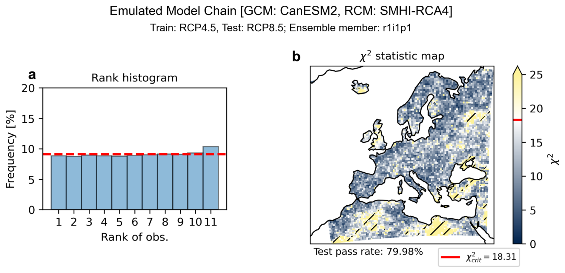
Figure 3 Evaluation of example model chain (RCM: SMHI-RCA4, GCM: CanESM2). The rank histogram based on all RCM grid points, where the red dash line indicates the ideal even distribution (a) and χ² test for rank histogram flatness at the RCM grid-point level (b). The hatched area in the χ² statistic map represents regions that fail the χ² test (i.e., ${\mathit{\chi }}^{\mathrm{2}}>{\mathit{\chi }}_{\mathrm{crit}}^{\mathrm{2}}$).

5.3 Evaluation of the probabilistic RCM emulator

The validation of the example GCM-RCM model chain (RCM: SMHI-RCA4, GCM: CanESM2) is shown in Fig. 3. The rank histogram (Fig. 3a) shows spatially-aggregated results, where the flatness of the rank histogram indicates overall reliable performance of the RCM emulator. The χ² test, applied at the grid-point level, shows that 80 % of RCM grid points exhibit significant rank uniformity, indicating generally reliable performance at the RCM grid-point level as well (Fig. 3b).

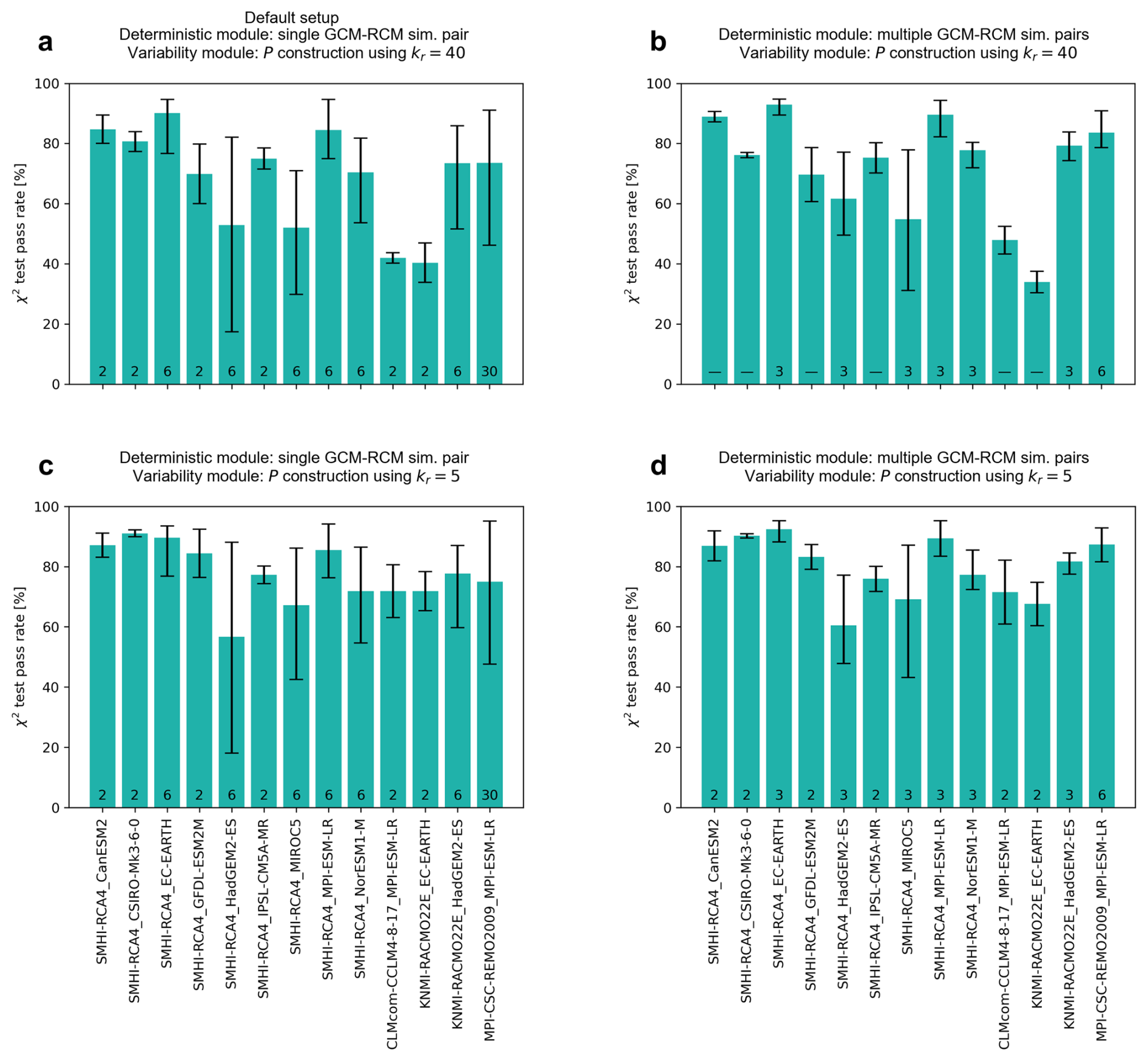
Figure 4 Comparison of training setups: χ² test pass rates across different GCM-RCM model chains. The x-axis lists the model chains, formatted as RCM-name_GCM-name. The number above each chain indicating the total validation experiments conducted. A dash (–) denotes cases where the sensitivity experiment could not be applied to a model chain due to data availability. In such cases, the experiment has no effect on the model chain, and the performance shown corresponds to the default setup. The prior covariance matrix P is constructed using residuals from the k_r nearest RCM simulations, determined by the Euclidean distance between their $\mathrm{diag}\left({\widehat{\mathbf{\Sigma }}}_{\mathrm{RCM}}^{\mathrm{res}}\right)$ and that of the training set. Here, k_r = 40 corresponds to the total number of available residuals of RCM simulations.

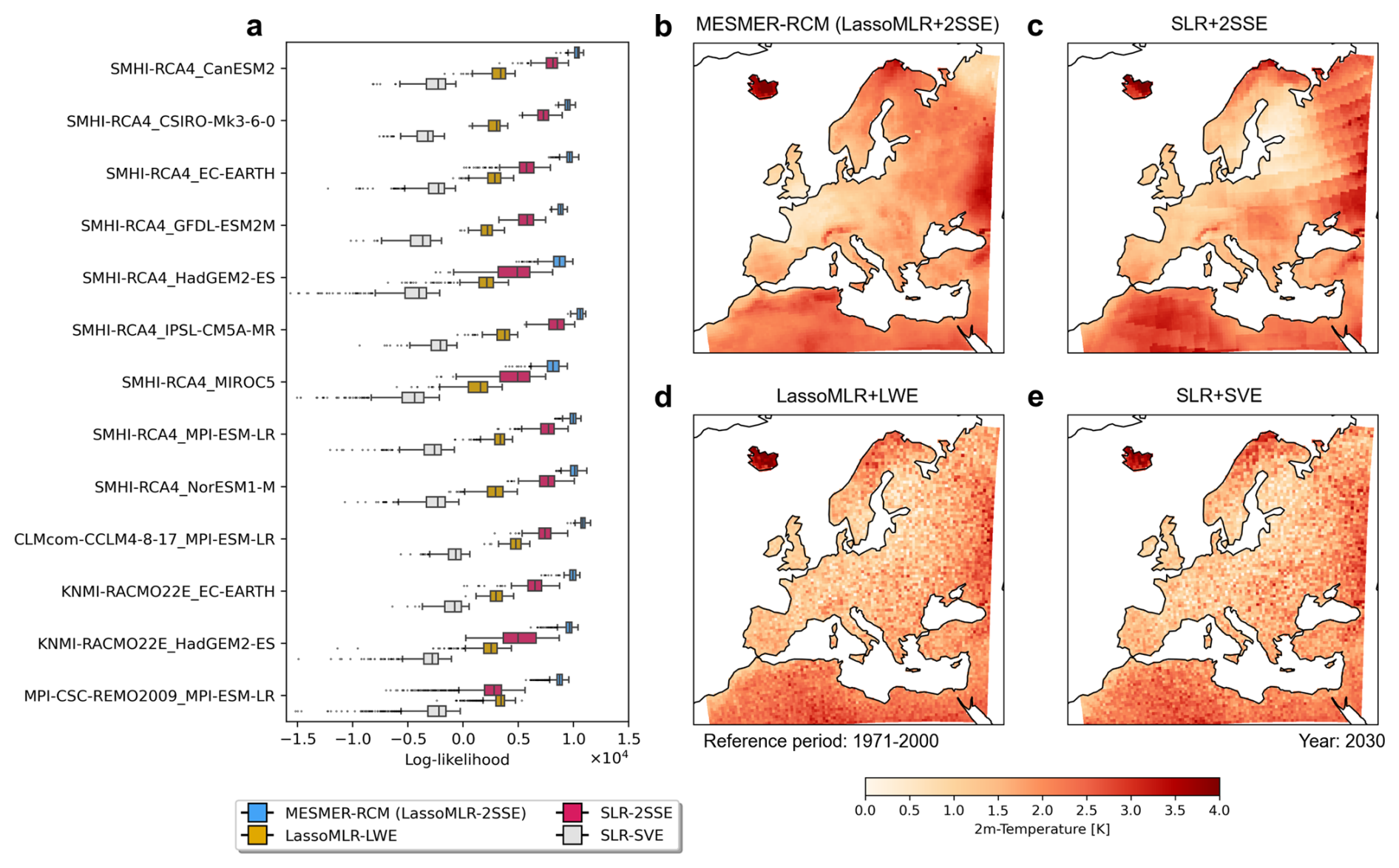
Figure 5 Comparison of MESMER-RCM with benchmark methods based on the log-likelihood of the RCM emulation, computed under a multivariate normal assumption from the spatial Gaussian distribution. (a) Yearly log-likelihood test performance aggregated into boxplots for each emulator across training–testing experiments of individual model chains. LassoMLR: lasso multiple linear regression; 2SSE: Two-stage shrinkage estimator; SLR: simple linear regression; LWE: Ledoit–Wolf estimator; SVE: sample variance estimator. (b–e) Example of emulation from MESMER-RCM and benchmark methods for the CanESM2-SMHI-RCA4 model chain, with emulators trained on RCP4.5 and tested on RCP8.5.

Extending the validation to all GCM-RCM model chains (Fig. 4), we observe fluctuations in the χ² test pass rate across different model chains, with a relatively large spread within individual chains. The example model chain SMHI-RCA4_CanESM2 is one of the better performing ones, while e.g. KNMI-RACMO22E_EC-EARTH only has a pass rate of 40 %. This fluctuation can be largely understood by our conducted sensitivity experiments. Comparing to default setup, training the deterministic response module in multiple instead of a single simulation pairs (Fig. 4b) improves the robustness of the scaling coefficients, which reduces bias in temperature trend projections. The resulting spread of χ² pass rates across validation experiments for each individual model chain is considerably lower. For example, in MPI-CSC-REMO2009_MPI-GCM-LR, the average χ² test pass rate increases by 10 % compared to default setup, while the spread decreases from ±20 % to ±5 %. The next sensitivity experiment revisits the residual variability module, using a physically consistent subset of concatenated RCM residuals to construct the prior P (Fig. 4c). This improves the statistical representation of residual variability, leading to higher average χ² test pass rates. For instance, the pass rate increases by 30 % for KNMI-RACMO22E_HadGEM2-ES and CLMcom-CCLM4-8-17_MPI-ESM-LR. Due to limited data availability, the construction of prior P faces a trade-off between physical consistency and numerical stability. In cases where stability is compromised, the emulator may suffer from distortion due to ill-conditioned sampling. Nevertheless, this sensitivity experiment highlights the potential to alleviate this trade-off by identifying and incorporating diverse, physically consistent model chains into the construction of P, thereby improving the sampling of the residual variability. Finally, the combined approach (Fig. 4d) shows a clear additive improvement in RCM emulation, highlighting the complementary strengths of training strategies indicated by our sensitivity experiments (Fig. 4b–c). These results reveals that the observed inter-model performance variability primarily stems from unevenly distributed GCM–RCM training data, and the emulator performance is generally robust when trained with well-prepared inputs.

We further assess MESMER-RCM's ability to emulate distribution of RCM reference using the log-likelihood, and compare it with different benchmarks (Fig. 5). Overall, MESMER-RCM provides more accurate and stable estimation of the RCM reference distribution compared to the benchmark methods, for all GCM-RCM model chains (Fig. 5a). The emulation generated by MESMER-RCM shows higher fidelity and physical plausibility (Fig. 5b). Comparing MESMER-RCM and SLR-2SSE, the simple linear regression as a nearest-neighbor method often leads to blocky artifacts (Allebach, 2005), which leaves behind the GCM grid texture and results in less smooth temperature fields (Fig. 5c). This distortion of temperature fields reflects a form of underfitting, which can be effectively improved by adding predictors and normalization using LassoMLR. Comparing MESMER-RCM and LassoMLR-LWE, the latter generates emulations with a noisy texture (Fig. 5d), because the sample covariance matrix is excessively shrunk to the unit matrix in LWE due to the high rank deficiency of the sample covariance matrix. MESMER-RCM has an advantage in this high-dimensional setting because the residual variability module adopts a more physically plausible prior for the shrinkage target and complement with two stage shrinkage procedure for ensuring numerical stability. This leads to a more favorable bias–variance trade-off by reducing estimation error while adding less bias.

6 Conclusions

This study develops a probabilistic RCM emulator, MESMER-RCM, which demonstrates reliable performance in emulating annual 2 m temperature projections over European land. MESMER-RCM is capable of exploring regional-scale warming under various scenario pathways and sampling internal RCM variability. Its modular structure enhances model interpretability and ensures computational efficiency, offering a simpler yet effective alternative to commonly used deep learning approaches. MESMER-RCM has the potential to be extended to other regions provided adequate simulation data are available. Our sensitivity experiments further underscore that emulator behavior depends strongly on the training data and that a sufficiently large set of GCM–RCM simulations is essential for building robust RCM emulators.

Future work on MESMER-RCM will leverage its ability to generate high-resolution ensemble projections from coarse-resolution data. Specifically, MESMER-RCM can be further integrated with GCM emulators to form a GCM-RCM emulator chain, adding value to GCM emulators by enhancing their spatial resolution. For instance, MESMER generates spatially resolved annual mean temperature fields from arbitrary global mean temperature inputs. Coupling MESMER with MESMER-RCM enables regional climate projections across a wide range of GCM–RCM combinations and scenario pathways, thereby facilitating comprehensive what-if analysis. Such a framework holds strong potential for informing regional climate risk assessments and supporting policy-relevant decision-making.