Elucidating the performance of data assimilation neural networks for chaotic dynamics

In supervised data assimilation machine learning emulation, the training data contain targets produced by an existing data assimilation scheme, such as analysis increments. By contrast, data assimilation networks were recently proposed to learn the analysis operator while they are embedded in the forecast–analysis cycle: their only targets are the true trajectory and the observations thereof. They are therefore trained to produce a stable and accurate sequential estimator, rather than to reproduce the output of a prescribed data assimilation algorithm. Conceptually more fundamental, yet computationally more challenging, such learned data assimilation scheme was shown to achieve accuracy comparable to that of the ensemble Kalman filter when applied to low-order chaotic dynamics. Strikingly, the same accuracy can be reached with a single state forecast instead of an ensemble, hence bypassing the need to explicitly represent forecast uncertainty.

In this study, we extend the investigation of such learned analysis operators beyond the preliminary experiments reported so far. First, we analyse the emergence of local patterns encoded in the operator, which accounts for the remarkable scalability of the approach to high-dimensional state spaces. Second, we assess the performance of the learned operators in stronger nonlinear regimes of the chaotic dynamics. We show that they can match the efficiency of the iterative ensemble Kalman filter, the baseline in this context, while avoiding the need for nonlinear iterative optimisation. Throughout the paper, we seek underlying reasons for the efficiency of the approach, drawing on insights from both machine learning and nonlinear data assimilation.

1 Introduction

Accurate prediction of geophysical flows relies on the continual correction of model trajectories using observations. This sequential data assimilation (DA) process is essential in high-dimensional chaotic systems, where errors amplify rapidly and model imperfections accumulate over time (Kalnay, 2003; Asch et al., 2016; Carrassi et al., 2018). In operational meteorology and oceanography, ensemble-based Kalman filters and ensemble variational methods provide reliable and well-understood frameworks for these updates, but they remain computationally demanding and rely on explicit representations of flow-dependent forecast error covariances.

Recent developments have suggested that part of this complexity can be replaced by learned analysis operators. In supervised DA machine learning emulation, the training dataset contains targets produced by an existing DA scheme, such as analysis increments (e.g., Härter and de Campos Velho, 2012; Cintra and de Campos Velho, 2018; Maddy et al., 2024). By contrast, one could learn the analysis operator while it is embedded in the forecast–analysis cycle: its only targets are the true trajectory and the observations thereof (McCabe and Brown, 2021). Such analysis operator is therefore trained to produce a stable and accurate sequential estimator, rather than to reproduce the output of a prescribed DA algorithm. Within this latter approach, termed data assimilation networks (DANs, Boudier et al., 2023), a surprising result has emerged: as demonstrated by Bocquet et al. (2024), a learned analysis operator can match the accuracy of a well-tuned ensemble Kalman filter (EnKF) even when it uses only single forecast trajectories, without any ensemble. This result challenges the long-standing assumption that explicit ensemble representations are indispensable to estimate flow-dependent uncertainties in chaotic systems.

Explaining this phenomenon is a central question for DA methodology. Initial investigations suggest that the learned operator implicitly reconstructs aspects of the analysis error covariances normally diagnosed from an ensemble, effectively uncovering key uncertainty directions from the forecast state alone (Bocquet et al., 2024). This behaviour is consistent with viewing the full DA cycle as a random dynamical system, for which generalised forms of the multiplicative ergodic theorem (Oseledec, 1968) offer a state-dependent structure linking model trajectories to dominant error-growth directions. At the same time, numerical experiments show that the neural network is likely to identify local patterns rather than memorising global states, which explains why its performance scales to larger systems and remains robust across different model dimensions.

This paper deepens the investigation of these mechanisms. In Sect. 2, we dive into the methodology of DANs, and recall the main results and questions raised in Bocquet et al. (2024). In Sect. 3, building on a more thorough analysis of the performance dependence on the batch size, dataset length, and the number of assimilation cycles used during backpropagation, we study how the operator behaves when interpreted as a diagnostic of uncertainty, and we propose methods to expose and interpret the local structures it extracts. In Sect. 4, we test the limits of the approach in more strongly nonlinear regimes, where the iterative ensemble Kalman filter (Sakov et al., 2012) and its generalisations often serve as the most accurate baselines. We show that the learned operator can reach comparable performance without requiring an ensemble or a nonlinear optimisation, and we offer a data assimilation-based interpretation for this ability. Section 5 presents our conclusions. Supporting numerical and mathematical results are collated in the appendices of this paper.

Throughout the paper, we will illustrate our results with the Lorenz-96 model (L96, Lorenz and Emanuel, 1998). More broadly, our goal is not only to document the performance of the learned analysis operators but also to clarify the mechanisms that underlie them, thereby contributing to the growing theoretical understanding of how deep learning and sequential data assimilation interact in chaotic geophysical systems (Cheng et al., 2023).

2 Theory and methods

In this section, we provide a deeper description of the problem, its context, and its mathematical formulation.

2.1 Sequential data assimilation for chaotic dynamics

Mathematically, data assimilation (DA), and in particular filtering algorithms, are meant to accurately estimate the state vector ${\mathbf{x}}_k^{\mathrm{t}}\in {\mathbf{E}}_{\mathrm{x}}\stackrel{\Delta }{=}{\mathbb{R}}^{N_{\mathrm{x}}}$ of a physical system, where “t” stands for truth, at times t_k for $k=\mathrm{1},\mathrm{\dots },K$ along a trajectory of the dynamical system. These states are evolved according to

$$\begin{array}{}\text{(1a)}& {\mathbf{x}}_{k+\mathrm{1}}^{\mathrm{t}}=\mathcal{M}\left({\mathbf{x}}_k^{\mathrm{t}}\right),\end{array}$$

where ℳ is the integrated model over $t_{k+\mathrm{1}}-t_k={\mathrm{\Delta }}_t$. The dynamical system ℳ is assumed to be chaotic, such as for most geofluids, which is a prime incentive for frequently updating our knowledge of the system. It is furthermore assumed ergodic and autonomous, i.e. does not explicitly depend on time. Furthermore, the physical system is observed through

$$\begin{array}{}\text{(1b)}& {\mathbf{y}}_k={\mathcal{H}}_k\left({\mathbf{x}}_k^{\mathrm{t}}\right)+{\mathit{\epsilon }}_k,{\mathit{\epsilon }}_k\sim \mathcal{N}(\mathbf{0},{\mathbf{R}}_k),\end{array}$$

where ${\mathbf{y}}_k\in {\mathbf{E}}_{\mathrm{y}}^k\stackrel{\Delta }{=}{\mathbb{R}}^{N_{\mathrm{y},k}}$ is the observation vector at t_k obtained from the hidden state ${\mathbf{x}}_k^{\mathrm{t}}$ via an observation operator ℋ_k, and perturbed by a white-in-time Gaussian noise ε_k of mean 0 and covariance matrix R_k. This very common but simplified formulation of the filtering problem with additive Gaussian noise is sufficient for the goals of this paper.

A filtering DA scheme estimates the hidden state ${\mathbf{x}}_k^{\mathrm{t}}$ at t_k from the observations available up to that time. The analysis ${\mathbf{x}}_k^{\mathrm{a}}$ is a point estimator, such as the posterior mean or maximum a posteriori estimate, of the conditional probability density function $p\left({\mathbf{x}}_k^{\mathrm{t}}\right|{\mathbf{y}}_k,{\mathbf{y}}_{k-\mathrm{1}},\mathrm{\dots },{\mathbf{y}}_{\mathrm{1}})$. A sequential filtering DA scheme infers ${\mathbf{x}}_k^{\mathrm{a}}$ from y_k and from background information about the state at t_k−1 (possibly brought forward to t_k using ℳ).

2.2 Learning the data assimilation analysis

2.2.1 Training scheme

The approach developed in Bocquet et al. (2024), subsequently referred to as Boc24, in the wake of McCabe and Brown (2021) and Boudier et al. (2023) is summarised in the following since it is the foundation of the present paper. The analysis step of the DA scheme is assumed to be given by the (incremental) analysis operator a_θ, typically a (deep) neural network, which depends on a set of weights and biases, stacked in the θ vector, and which is defined, at time t_k, through

$$\begin{array}{}\text{(2a)}& {\displaystyle }{\mathbf{x}}_k^{\mathrm{a}}& {\displaystyle }={\mathbf{x}}_k^{\mathrm{f}}+{\mathbf{a}}_{\mathit{\theta }}({\mathbf{x}}_k^{\mathrm{f}},{\mathbf{H}}_k^{⊺}{\mathbf{R}}_k^{-\mathrm{1}}{\mathit{\delta }}_k),\text{(2b)}& {\displaystyle }{\mathit{\delta }}_k& {\displaystyle }\stackrel{\Delta }{=}{\mathbf{y}}_k-{\mathcal{H}}_k\left({\mathbf{x}}_k^{\mathrm{f}}\right),\end{array}$$

where δ_k is the innovation, ${\mathbf{x}}_k^{\mathrm{a}}$ is the analysis state mentioned previously, and ${\mathbf{x}}_k^{\mathrm{f}}$ is the forecast state, to be defined shortly. H_k is the tangent linear operator of ℋ_k. Should a_θ be a function of δ_k rather than ${\mathbf{H}}_k^{⊺}{\mathbf{R}}_k^{-\mathrm{1}}{\mathit{\delta }}_k$, it could only handle static observation configurations, and would require to be retrained whenever that configuration changes. Although not the focus of this paper, this important issue is circumvented here by using the mapping from observation to state space ${\mathbf{H}}_k^{⊺}{\mathbf{R}}_k^{-\mathrm{1}}$, such that both inputs of a_θ are in the same static state space E_x. For compactness, we define the projected innovation

$$\begin{array}{}\text{(2c)}& {\mathit{\zeta }}_k\stackrel{\Delta }{=}{\mathbf{H}}_k^{⊺}{\mathbf{R}}_k^{-\mathrm{1}}{\mathit{\delta }}_k={\mathbf{H}}_k^{⊺}{\mathbf{R}}_k^{-\mathrm{1}}({\mathbf{y}}_k-{\mathbf{H}}_k({\mathbf{x}}_k^{\mathrm{f}}\left)\right).\end{array}$$

The DAN analysis operator thus receives two fields in state space, ${\mathbf{x}}_k^{\mathrm{f}}$ and ζ_k.

In the DA forecast step, the analysis state is propagated to the subsequent date through

$$\begin{array}{}\text{(3)}& {\mathbf{x}}_{k+\mathrm{1}}^{\mathrm{f}}=\mathcal{M}\left({\mathbf{x}}_k^{\mathrm{a}}\right).\end{array}$$

The operator a_θ is trained by comparing the analysis states to the true states, through the loss

$$\begin{array}{}\text{(4)}& \mathcal{L}\left(\mathit{\theta }\right)=\sum _{r=\mathrm{1}}^{N_{\mathrm{r}}}\sum _{k=\mathrm{1}}^{N_{\mathrm{c}}}{∥{\mathbf{x}}_k^{\mathrm{t},r}-{\mathbf{x}}_k^{\mathrm{a},r}\left(\mathit{\theta }\right)∥}^{\mathrm{2}},\end{array}$$

where ${\mathbf{x}}_k^{\mathrm{t},r}$ are the state vectors of the true trajectory, indexed by the time index k and a trajectory index r as N_r of them are processed concurrently in the training of a_θ.

The N_c parameter counts the number of cycles of each DA run. It can potentially be infinite since trajectories can be generated online as the training progresses. The implementation of similar losses is detailed in McCabe and Brown (2021), Boudier et al. (2023), and Sect. II of Boc24. This notably requires to truncate backpropagation in time (Tang and Glass, 2018) which restricts the dependence on θ over N_iter≪N_c cycles only so as to reduce the computational cost and the excessive GPU memory (VRAM) requirement. Alternative losses based on probability density functions (pdf) diagnostics are possible and discussed in, e.g., Boudier et al. (2023). We have shown that a semi-supervised loss where the training dataset reduces to the sparse and noisy observations is also possible by generalising a proposal of McCabe and Brown (2021), but is out of the scope of this paper.

2.2.2 Accuracy of the discovered data assimilation scheme

Note that an ensemble variant of the update Eq. (2) was first considered in McCabe and Brown (2021), Boudier et al. (2023), and later by Boc24. Experimenting with the same low-order chaotic model, they found an accuracy of the learned DA scheme close to that of a well-tuned EnKF, which is per se very promising. In those experiments, DAN is built on an ensemble of analyses and forecasts. However, Boc24 demonstrated that this accuracy remains unchanged when these ensembles are reduced to a single state. This is a very surprising result since it is expected (and verified in the L96 context) that the EnKF-like methods critically relying on an ensemble representing the errors of the day, have a significant edge over other sequential DA methods that leverage a single forecast state such as 3D-Var and 4D-Var (see Bocquet and Sakov, 2013, for a quantitative comparison with the same model). This explains why numerical weather prediction (NWP) centres operating 4D-Var actually rely on an ensemble of such 4D-Var, a technique called EDA (see, e.g., Chap. 7 in Asch et al., 2016; Bannister, 2017, and references within), or use information from a concurrent EnKF (Buehner et al., 2015). That is why achieving the accuracy of a well-tuned EnKF with a single forecast state should have far-reaching implications on the mechanisms and designs of DA algorithms for chaotic dynamics, and warrants investigating the reason for such feat.

2.3 Investigating the reason for this efficiency

To unveil the mechanisms leveraged by the learned analysis operator to achieve this accuracy, Boc24 performed a linearisation of the operator a_θ in the projected innovation ζ:

$$\begin{array}{}\text{(5)}& {\mathbf{a}}_{\mathit{\theta }}(\mathbf{x},\mathit{\zeta })\approx {\mathbf{P}}^{\mathrm{a}}\left(\mathbf{x}\right)\mathit{\zeta },\end{array}$$

where P^a(x) is the resulting linear operator that acts on ζ. Comparing with the linearisation of the classical Kalman update, it must coincide with the analysis error covariance matrix which could be associated by formal analogy to the learned analysis operator a_θ, hence the notation. This covariance matrix was numerically obtained in Boc24 through a linear regression in between a large ensemble of ζ samples (corresponding to the projected innovations ${\mathbf{H}}^{⊺}{\mathbf{R}}^{-\mathrm{1}}\mathit{\delta }$) and a_θ(x,ζ) outputs. It was found that this error covariance matrix is remarkably close to that of a well-tuned EnKF, especially for its dominant eigenvectors (which carry most of the uncertainty in the analysis).

Hence, the performance of DAN, as reported in Boc24, must be to a large extent due to its ability to infer flow-dependent effective analysis error covariances from the forecast state, as revealed by the local dependence of a_θ(x^f,ζ) on the projected innovation ζ. Such an ability is pivotal for maintaining the accuracy of sequential DA over time. In the present paper, we will sometimes reason in terms of the forecast error covariance matrix P^f in place of P^a, since the flow dependence is more naturally encoded in P^f, while P^a is obtained after conditioning on the observations. Moreover, in the linear/Gaussian case, these two covariance matrices are straightforwardly related by

$$\begin{array}{}\text{(6)}& {\left({\mathbf{P}}^{\mathrm{a}}\right)}^{-\mathrm{1}}=({\mathbf{P}}^{\mathrm{f}}{)}^{-\mathrm{1}}+{\mathbf{H}}^{⊺}{\mathbf{R}}^{-\mathrm{1}}\mathbf{H},\end{array}$$

assuming invertibility of the error covariance matrices. Beyond the linear/Gaussian case, perturbing the innovations and applying DAN can generate an empirical analysis ensemble; propagating this ensemble with the model ℳ then provides a way to diagnose the corresponding forecast error covariances.

Other alternatives to ensemble forecasting to estimate the flow-dependent error statistics, such as deriving the dynamics of the statistical moments of the errors (Pannekoucke et al., 2016, 2018), or estimating these dynamics through machine learning (Pannekoucke and Fablet, 2020; Sacco et al., 2024; Lu, 2025) are either numerically very costly or in their infancy.

Boc24 conjectured that DAN's ability to assess the flow-dependent error statistics can be fundamentally explained by the existence of an ad-hoc multiplicative ergodic theorem (MET). From the seminal MET result by Oseledec (1968), we know that, for an autonomous ergodic dynamical system such as ℳ, there exists, for almost every state on the attractor, a measurable mapping from the state to the corresponding Oseledets subspaces. Generalising, one can consider the whole sequential DA process as a dynamical system on its own (Carrassi et al., 2008). Such DA process is not autonomous because it indirectly depends on the truth trajectory and the time-dependent observation operators. Moreover, it is a random process, since stochasticity is injected via the noisy observations. It turns out that generalised variants of the MET for non-autonomous random dynamics are possible (Arnold, 1998; Chekroun et al., 2011; Flandoli and Tonello, 2021; Ghil and Sciamarella, 2023) and are potentially applicable to such sequential DA process. Hence, Boc24 conjectured that a_θ can exploit such state-dependent information to infer an effective analysis error covariance matrix, together with how to process this information and combine it with the innovation.

To explain the efficiency of a_θ, one may suggest that the neural network memorises global configurations of the forecast state, with very limited ability to generalise. On the contrary, Boc24 showed via indirect scaling experiments that a_θ learns to identify local patterns (i.e. with a limited range in space), which was made easier by the architecture of a_θ being a residual convolutional neural network. Indeed, when the dimension N_x of the L96 state space is increased, and new a_θ operators are learned but with a fixed number of weights and biases of the backbone architecture, the accuracy remains that of a well tuned EnKF of matching dimension. Yet, in the large N_x limit, a_θ with the same number of degrees of freedom should not be able to memorise increasingly numerous global patterns. Hence, a_θ must extract local patterns, and a limited number of them. This is further supported by learning a_θ with the original L96 dimension, N_x=40, but applying it to L96 with significantly different N_x in successful DA runs (this is allowed by the convolutional architecture which does not explicitly depend on N_x), performing on par with a well tuned EnKF. Hence, any local pattern learned in the case N_x=40, must still be spotted by a_θ where N_x≠40. This outcome is consistent with the existence of such local patterns, since L96 is an extensive model when N_x is increased, with the number of nonlinear interacting waves in the model being proportional to N_x. This neat scalability has limitations. If increasing the dimension changed the local statistics or local dynamical balances of the model, for example through a substantial change of spectral slope or local instability mechanisms, a DAN trained at the smaller dimension should not be expected to generalise without fine-tuning, additional training, or architectural adaptation.

3 Exploration of data assimilation networks

With the previously established context in mind, we now explore what DANs (a_θ) learn in mildly nonlinear regimes. The neural network associated to a_θ implements Eq. (2). The architecture for a_θ we choose in the present paper is the same as the one reported in Boc24, i.e. a simple residual convolutional neural network that accounts well for the spatial homogeneity of L96 (and hence its statistical stationarity). For the sake of self-sufficiency, Appendix A describes this architecture. All the training tasks are carried out over a training dataset with a minimisation of the loss controlled by computing the loss over a validation dataset.

3.1 Numerical setup

The numerical experiments of the present paper are performed on L96, a chaotic model abundantly used for benchmarking new sequential data assimilation algorithms. As a reminder, L96 represents a mid-latitude zonal circle of the global atmosphere. It is governed by N_x=40 ordinary differential equations:

$$\begin{array}{}\text{(7)}& {\displaystyle \frac{\mathrm{d}{x}_n}{\mathrm{d}t}}=(x_{n+\mathrm{1}}-x_{n-\mathrm{2}})x_{n-\mathrm{1}}-x_n+F,\end{array}$$

where F=8, and with cyclic boundary conditions. The resulting model is chaotic with 13 positive and 1 neutral Lyapunov exponents. Its Lyapunov time, defined as the inverse of the first Lyapunov exponent, is about 0.60, which corresponds to 3 d of a typical weather forecasting model (Lorenz and Emanuel, 1998).

Although the results are generalisable to sparse observations, the observation operator will mostly be chosen to be the identity ${\mathbf{H}}_k\stackrel{\Delta }{=}{\mathbf{I}}_{\mathrm{x}}$. The observations are read off the true state and perturbed with an unbiased white-in-time Gaussian additive noise of covariance matrix ${\mathbf{R}}_k\stackrel{\Delta }{=}{\mathbf{I}}_{\mathrm{x}}$ following Eq. (1b). The time-step between observation batches and updates is set to ${\mathrm{\Delta }}_t=t_{k+\mathrm{1}}-t_k=\mathrm{0.05}$ for all experiments with the exception of Sect. 4.1. This will be our reference DA setup. Examples of alternative sparseness and noise levels are given in Boc24, but here as well when relevant.

All the a_θ operators learned in this configuration are subsequently evaluated with a time-averaged analysis root mean square error (RMSE) whose mean square is averaged over the N_x variables. This RMSE is assessed over a dataset of independent test trajectories, similarly to traditional DA twin experiments. For brevity, this score computed for each trained DAN scheme will simply be called test RMSE of the DAN scheme in the rest of this paper.

In this configuration, running a well-tuned EnKF in a twin experiment and comparing its analysis to the truth yield a test RMSE between 0.18 and 0.20 depending on the ensemble size N_e and whether localisation is used or not. By contrast, a basic but well-tuned 3D-Var or a reasonably short window basic but well tuned 4D-Var yields a test RMSE of about 0.40. They largely underperform the EnKF because they fail to capture the errors of day (Bocquet and Sakov, 2013; Fillion et al., 2018).

In order to be able to perform a large number of training experiments on a limited number of GPUs and limited VRAM, we carried out a sensitivity study on the batch size, the size of the datasets, and the backpropagation truncation, beyond the restricted set of experiments reported in Boc24. Since the results are technical and mostly of practical interest, they are reported in Appendix B. They were nonetheless instrumental in obtaining the main numerical results of this paper.

3.2 Linearisation in the innovations

In this section, we discuss the relevance of expanding a_θ linearly in the innovations, as in Eq. (5). We recall that the focus is on the analysis step of the DAN process, where N_e=1, i.e. a single forecast state is propagated in between updates. Under the additional Gaussian and quasi-linear assumptions used in this subsection, a close to optimal analysis associated with the Kalman update is the posterior mean which coincides with the maximum a posteriori of the conditional pdf, hence by the minimum of the cost function associated to the analysis. In the following, the observation operator is assumed linear (or linearised) for simplicity, i.e. $\mathcal{H}\stackrel{\Delta }{=}\mathbf{H}$.

3.2.1 A Gaussian standpoint on the analysis

Here, we further assume that the background errors are Gaussian. Nonetheless, as opposed to a basic 3D-Var, the background error covariance matrix depends on the forecast state. Hence, the typical analysis cost function associated to the analysis at any given time step has the form:

$$\begin{array}{}\text{(8)}& \mathcal{J}\left(\mathbf{x}\right)={\displaystyle \frac{\mathrm{1}}{\mathrm{2}}}{∥\mathbf{y}-\mathbf{Hx}∥}_{{\mathbf{R}}^{-\mathrm{1}}}^{\mathrm{2}}+{\displaystyle \frac{\mathrm{1}}{\mathrm{2}}}\Vert \mathbf{x}-{\mathbf{x}}^{\mathrm{f}}{\Vert }_{{\left({\mathbf{P}}^{\mathrm{f}}\left({\mathbf{x}}^{\mathrm{f}}\right)\right)}^{-\mathrm{1}}}^{\mathrm{2}}.\end{array}$$

As a consequence, 𝒥 is quadratic in x, strictly convex, and its minimum argument is (Daley, 1991)

$$\begin{array}{ll}{\displaystyle }{\mathbf{x}}^{\mathrm{a}}& {\displaystyle }={\mathbf{x}}^{\mathrm{f}}+[{\mathbf{H}}^{⊺}{\mathbf{R}}^{-\mathrm{1}}\mathbf{H}+({\mathbf{P}}^{\mathrm{f}}\left({\mathbf{x}}^{\mathrm{f}}\right){)}^{-\mathrm{1}}{]}^{-\mathrm{1}}{\mathbf{H}}^{⊺}{\mathbf{R}}^{-\mathrm{1}}(\mathbf{y}-{\mathbf{Hx}}^{\mathrm{f}})\\ \text{(9)}& {\displaystyle }& {\displaystyle }={\mathbf{x}}^{\mathrm{f}}+{\mathbf{P}}^{\mathrm{a}}\left({\mathbf{x}}^{\mathrm{f}}\right)\mathit{\zeta },\end{array}$$

where the projected innovation ζ has been defined by Eq. (2c). Equation (9) matches the linearisation Eq. (5). The purpose of this derivation is to show that, under Gaussian/quasi-linear assumptions, DAN is likely to solve the optimisation problem Eq. (8), that its update follows Eq. (9), and that its Jacobian with respect to ζ plays the role of an effective analysis error covariance matrix P^a(x^f). Whether this local interpretation is sufficient is then tested numerically.

3.2.2 Numerical evidence

To numerically test whether such a linearisation is a good approximation for a_θ, we created a modified DAN which explicitly learns an effective map x^f↦P^a(x^f) and linearly combines it with the projected innovations, with the goal to strictly follow the update equation Eq. (9). Details on our scalable implementation of Eq. (9), for such a DAN linear in the projected innovations (from now on called linear-in-ζ DAN), can be found in Appendix C. One must keep in mind that this linear-in-ζ DAN is numerically inefficient since it requires to build a representation of the covariance matrix P^a before being applied to the projected innovations, an operation which is likely to be achieved with our standard DAN without ever computing P^a explicitly.

This deconstruction of a_θ directly connects with the heuristic developed by Sacco et al. (2024) and Sakov (2025), where the mapping x^f↦P^f(x^f) is learned and then successfully used within a classical EnKF. Numerically, the linear-in-ζ DAN scheme turns out to be as accurate as a well-tuned EnKF with N_e=40 in the reference setup (Δ_t=0.05 in particular), with a test RMSE of ∼0.19, which is in line with the results by Sacco et al. (2024) and Sakov (2025). Hence, we can claim that the good performance of DAN in this mildly nonlinear regime importantly relies on the (implicit) estimation of the mapping x^f↦P^f(x^f), and subsequently x^f↦P^a(x^f).

3.2.3 On the importance of the x^f↦P^f(x^f) map

Let us focus on Sakov (2025), whose algorithmic constructions targeted at estimating P^f(x^f) are especially transparent and whose numerical tests were carried out in the reference setup described in Sect. 3.1. Their Algorithm A1 proceeds as follows: (i) the state x^f is backtracked by T time steps; (ii) the tangent linear model, evaluated along the resulting state trajectory from t_−T to t₀, is applied to a matrix of state perturbations εI_x; and (iii) the resulting perturbations at time t₀ are used to estimate P^f(x^f). This procedure is closely related to the Assimilation in the Unstable Space (AUS) methods (Palatella et al., 2013; Carrassi et al., 2022), since for sufficiently large T the output of the tangent linear model at t₀ provides a square-root factor of the backward Lyapunov vectors. But it is already sufficient to yield a competitive analysis relying on the errors of the day estimated through P^f(x^f) which notably relies on a single state.

Algorithm A2 of Sakov (2025) also backtracks the state x^f by T time steps but differs in the subsequent step: instead of propagating perturbations, it applies a (square-root) Kalman filter to an initial covariance matrix ε²I_x from t_−T to t₀, yielding a more refined estimate of P^f(x^f) at t₀. This yields an even more accurate DA algorithm on par with a well tuned EnKF, again relying on P^f(x^f) assessed from a single state.

Bocquet et al. (2017) and Bocquet and Carrassi (2017) have laid the theoretical grounds to understand why these principled demonstrations are successful. Bocquet et al. (2017) focused on a degenerate Kalman filter, equivalent to an EnKF in Gaussian and quasi-linear conditions. In this setting, the covariance evolution is formally decoupled from the state update, with the important caveat that the forecast error covariance P^f depends on the state x^f at time t₀. Indeed, Bocquet et al. (2017) showed that, asymptotically (i.e. for large T), P^f depends on the system dynamics only through the Lyapunov vectors. By the MET, the corresponding Oseledets subspaces are measurable functions of the state x^f at t₀ (for almost every state on the attractor). Hence, following Bocquet et al. (2017), Algorithm A2 by Sakov (2025) can be directly interpreted as the single state-dependent covariance propagation of a degenerate Kalman filter. In the case of nonlinear dynamics, enforcing the dependence of the error covariance P^f on x^f is even more beneficial since the covariance evolution now explicitly depends on x^f.

These theoretical results and proof experiments provide a rationale for the existence of a map x^f↦P^f(x^f) and its importance in estimating the errors-of-the-day in DA schemes based on a single forecast state N_e=1.

3.3 Patterns

In this section, we visualise a footprint of the local patterns leveraged by DAN to make its inferences. To that end, we study the dependence of ${\mathrm{\nabla }}_{\mathit{\zeta }}{\mathbf{a}}_{\mathit{\theta }}(\mathbf{x},\mathit{\zeta }{)}_{|\mathit{\zeta }=\mathbf{0}}\approx {\mathbf{P}}^{\mathrm{a}}(\mathbf{x})$ on x, i.e. the forecast state. This can be seen as a linear-in-ζ sensitivity analysis of a_θ with respect to its inputs.

3.3.1 Mean marginal gain tensor

Specifically, the sensitivity analysis will focus on Jacobians of the analysis operator with respect to x:

$$\begin{array}{}\text{(10a)}& {\displaystyle }& {\displaystyle }\mathbf{\Gamma }(\mathbf{x},\mathit{\zeta })\stackrel{\Delta }{=}{\mathrm{\nabla }}_{\mathbf{x}}{\mathrm{\nabla }}_{\mathit{\zeta }}{\mathbf{a}}_{\mathit{\theta }}(\mathbf{x},\mathit{\zeta }),\text{(10b)}& {\displaystyle }& {\displaystyle }\mathbf{\Gamma }\left(\mathbf{x}\right)\stackrel{\Delta }{=}\mathbf{\Gamma }(\mathbf{x},\mathbf{0})={\mathrm{\nabla }}_{\mathbf{x}}{\mathrm{\nabla }}_{\mathit{\zeta }}{\mathbf{a}}_{\mathit{\theta }}(\mathbf{x},\mathit{\zeta }{)}_{|\mathit{\zeta }=\mathbf{0}}.\end{array}$$

Since Γ(x) is a proxy to ∇_xP^a(x) as per Eq. (5), Γ(x) can be interpreted as the marginal variation of P^a(x) when the forecast state x is perturbed. Under Gaussianity and linearity and assuming ${\mathbf{H}}^{⊺}{\mathbf{R}}^{-\mathrm{1}}={\mathbf{I}}_{\mathrm{x}}$, P^a(x) coincides with the Kalman gain. That is why we will call Γ(x) the marginal gain tensor, or simply marginal gain. Mathematically, this is a 3-tensor field, i.e. a map from the state space E_x to ${\mathbf{E}}_{\mathrm{x}}^{\mathrm{3}}$. Component-wise, using a conventional placement of indices, its definition reads

$$\begin{array}{}\text{(11)}& \left[\mathbf{\Gamma }\right(\mathbf{x}){]}_{ijl}\stackrel{\Delta }{=}{\left({\partial }_{x_l}{\partial }_{{\mathit{\zeta }}_j}{a}_{\mathit{\theta },i}(\mathbf{x},\mathit{\zeta })\right)}_{|\mathit{\zeta }=\mathbf{0}}.\end{array}$$

To mitigate the complexity in studying the map x↦Γ(x), we introduce the mean marginal gain, $\stackrel{\mathrm{‾}}{\mathbf{\Gamma }}$. This 3-tensor is defined as the average of Γ(x) over the K states of a long trajectory ${\mathcal{T}}_{\mathbf{x}}={\left\{{\mathbf{x}}_k^{\mathrm{t}}\right\}}_{k=\mathrm{1},\mathrm{\dots },K}\in {\mathbf{E}}_{\mathrm{x}}^K$ of the ℳ–based ergodic chaotic dynamics:

$$\begin{array}{}\text{(12)}& \stackrel{\mathrm{‾}}{\mathbf{\Gamma }}\stackrel{\Delta }{=}\langle \mathbf{\Gamma }\left(\mathbf{x}\right){\rangle }_{\mathbf{x}\in {\mathcal{T}}_{\mathbf{x}}}\underset{K\to \mathrm{\infty }}{=}\int \mathrm{d}\mathbf{x}\mathit{\pi }\left(\mathbf{x}\right)\mathbf{\Gamma }\left(\mathbf{x}\right)={\mathbb{E}}_{\mathbf{x}\sim \mathit{\pi }}\left[\mathbf{\Gamma }\left(\mathbf{x}\right)\right],\end{array}$$

where π is the invariant distribution of the ergodic chaotic dynamics.

As recalled in Sect. 2.3, ${\mathrm{\nabla }}_{\mathit{\zeta }}{\mathbf{a}}_{\mathit{\theta }}(\mathbf{x},\mathit{\zeta }{)}_{|\mathit{\zeta }=\mathbf{0}}\approx {\mathbf{P}}^{\mathrm{a}}(\mathbf{x})$ was heuristically estimated in Boc24 using samples of ζ followed by a linear regression. This estimation through a regression can be formally justified using the following argument. We wish to average ∇_ζa_θ(x,ζ) over the pdf ρ(ζ) of the projected innovations ζ, which is assumed to be a Gaussian with a positive-definite covariance matrix Σ_ρ. Then it can be shown that

$$\begin{array}{}\text{(13a)}& {\displaystyle }{\mathbb{E}}_{\mathit{\zeta }\sim \mathit{\rho }}\left[{\mathrm{\nabla }}_{\mathit{\zeta }}{\mathbf{a}}_{\mathit{\theta }}(\mathbf{x},\mathit{\zeta })\right]& {\displaystyle }=\int \mathrm{d}\mathit{\zeta }\mathit{\rho }\left(\mathit{\zeta }\right){\mathrm{\nabla }}_{\mathit{\zeta }}{\mathbf{a}}_{\mathit{\theta }}(\mathbf{x},\mathit{\zeta })\text{(13b)}& {\displaystyle }& {\displaystyle }={\mathbf{\Sigma }}_{\mathit{\rho }}^{-\mathrm{1}}{\text{Cov}}_{\mathit{\zeta }\sim \mathit{\rho }}\left[\mathit{\zeta },{\mathbf{a}}_{\mathit{\theta }}(\mathbf{x},\mathit{\zeta })\right],\end{array}$$

where $\text{Cov}\left[\cdot ,\cdot \right]$ is the covariance operator, and ${\mathbf{\Sigma }}_{\mathit{\rho }}^{-\mathrm{1}}$ operates on the first tensor factor. A proof is given in Appendix D, along with a generalisation to the case where Σ_ρ is only semi positive-definite, which is made necessary because the set $\mathit{\{}{\mathit{\zeta }}_k={\mathbf{H}}_k^{⊺}{\mathbf{R}}_k^{-\mathrm{1}}{\mathit{\delta }}_k{\mathit{\}}}_k$ may only span a subspace of E_x if H_k is not injective. This result is none other than Stein's lemma (Liu, 1994) applied to the Gaussian approximation of ρ and ${\mathbf{a}}_{\mathit{\theta }}(\mathbf{x},\cdot )$. It aligns with its original use in ensemble DA (Stordal et al., 2016; Raanes et al., 2019; Fillion et al., 2020) and with the connection established by Lemma 2 of Agarwal et al. (2021) between ${\mathbf{\Sigma }}_{\mathit{\rho }}^{-\mathrm{1}}{\text{Cov}}_{\mathit{\zeta }\sim \mathit{\rho }}\left[\mathit{\zeta },{\mathbf{a}}_{\mathit{\theta }}(\mathbf{x},\mathit{\zeta })\right]$, which is a perturbations-based estimator (Ribeiro et al., 2016), and a SmoothGrad estimator (Smilkov et al., 2017). In the limit where ζ, as a random vector, is concentrated around 0 and ρ can be approximated as Gaussian, which corresponds to the most common weak assimilation regime where the information content of the innovation is small compared to that of the background, we have

$$\begin{array}{}\text{(14a)}& {\displaystyle }{\mathbf{\Sigma }}_{\mathit{\rho }}^{-\mathrm{1}}{\text{Cov}}_{\mathit{\zeta }\sim \mathit{\rho }}\left[\mathit{\zeta },{\mathbf{a}}_{\mathit{\theta }}(\mathbf{x},\mathit{\zeta })\right]& {\displaystyle }=\int \mathrm{d}\mathit{\zeta }\mathit{\rho }\left(\mathit{\zeta }\right){\mathrm{\nabla }}_{\mathit{\zeta }}{\mathbf{a}}_{\mathit{\theta }}(\mathbf{x},\mathit{\zeta })\text{(14b)}& {\displaystyle }& {\displaystyle }\approx {\mathrm{\nabla }}_{\mathit{\zeta }}{\mathbf{a}}_{\mathit{\theta }}(\mathbf{x},\mathit{\zeta }{)}_{|\mathit{\zeta }=\mathbf{0}},\end{array}$$

which, with Eq. (13a), relates the integral form ${\mathbb{E}}_{\mathit{\zeta }\sim \mathit{\rho }}\left[{\mathrm{\nabla }}_{\mathit{\zeta }}{\mathbf{a}}_{\mathit{\theta }}\right(\mathbf{x},\mathit{\zeta }\left)\right]$ to the gradient form ${\mathrm{\nabla }}_{\mathit{\zeta }}{\mathbf{a}}_{\mathit{\theta }}(\mathbf{x},\mathit{\zeta }{)}_{|\mathit{\zeta }=\mathbf{0}}$ of the sensitivity of a_θ(x,ζ) with respect to ζ.

Building on this correspondance, we can connect the following mean marginal gain

$$\begin{array}{}\text{(15)}& \stackrel{\mathrm{̃}}{\mathbf{\Gamma }}\stackrel{\Delta }{=}{\mathbb{E}}_{\mathbf{x}\sim \mathit{\pi },\mathit{\zeta }\sim \mathit{\rho }}\left[\mathbf{\Gamma }\right(\mathbf{x},\mathit{\zeta }\left)\right]=\int \mathrm{d}\mathbf{x}\mathrm{d}\mathit{\zeta }\mathit{\pi }\left(\mathbf{x}\right)\mathit{\rho }\left(\mathit{\zeta }\right)\mathbf{\Gamma }(\mathbf{x},\mathit{\zeta }),\end{array}$$

defined from Eq. (10a) and more closely related to the DA process, to the mean marginal gain $\stackrel{\mathrm{‾}}{\mathbf{\Gamma }}$ as defined in Eq. (12):

$$\begin{array}{}\text{(16a)}& {\displaystyle }\stackrel{\mathrm{̃}}{\mathbf{\Gamma }}& {\displaystyle }={\mathbb{E}}_{\mathbf{x}\sim \mathit{\pi },\mathit{\zeta }\sim \mathit{\rho }}\left[\mathbf{\Gamma }(\mathbf{x},\mathit{\zeta })\right]\text{(16b)}& {\displaystyle }& {\displaystyle }={\mathbb{E}}_{\mathbf{x}\sim \mathit{\pi }}\left[{\mathrm{\nabla }}_{\mathbf{x}}{\mathbb{E}}_{\mathit{\zeta }\sim \mathit{\rho }}\left[{\mathrm{\nabla }}_{\mathit{\zeta }}{\mathbf{a}}_{\mathit{\theta }}(\mathbf{x},\mathit{\zeta })\right]\right]\text{(16c)}& {\displaystyle }& {\displaystyle }\approx {\mathbb{E}}_{\mathbf{x}\sim \mathit{\pi }}\left[{\mathrm{\nabla }}_{\mathbf{x}}{\mathrm{\nabla }}_{\mathit{\zeta }}{\mathbf{a}}_{\mathit{\theta }}(\mathbf{x},\mathit{\zeta }{)}_{|\mathit{\zeta }=\mathbf{0}}\right]\text{(16d)}& {\displaystyle }& {\displaystyle }={\mathbb{E}}_{\mathbf{x}\sim \mathit{\pi }}\left[\mathbf{\Gamma }\left(\mathbf{x}\right)\right]\text{(16e)}& {\displaystyle }& {\displaystyle }=\stackrel{\mathrm{‾}}{\mathbf{\Gamma }}.\end{array}$$

However, the empirical mean of Γ(x,ζ) from which to evaluate $\stackrel{\mathrm{̃}}{\mathbf{\Gamma }}$, and denoted $\widehat{\mathbf{\Gamma }}$, and which is the numerical estimation of the sensitivity out of a long enough DA run, may differ from both theoretical means $\stackrel{\mathrm{̃}}{\mathbf{\Gamma }}$ and $\stackrel{\mathrm{‾}}{\mathbf{\Gamma }}$. That is why we show in Appendix E how $\widehat{\mathbf{\Gamma }}$ approximates $\stackrel{\mathrm{̃}}{\mathbf{\Gamma }}$.

Note that Eq. (16a) is a simple point estimator, which formalises that the averaged Jacobian 𝔼_ζ[∇_ζa_θ(x,ζ)] is well approximated by ${\mathrm{\nabla }}_{\mathit{\zeta }}{\mathbf{a}}_{\mathit{\theta }}(\mathbf{x},\mathit{\zeta }){|}_{\mathit{\zeta }=\mathbf{0}}$ when the distribution of projected innovations is concentrated near zero. The Stein lemma, which provides a regression-based estimator of this average, is not required per se to ascertain Eq. (16a), but offers an alternative expression which we leverage in Appendix H.

3.3.2 Invariance and equivariance

An important way to reduce the computational cost and complexity of interpreting the mean marginal gain $\stackrel{\mathrm{̃}}{\mathbf{\Gamma }}$ is to exploit the symmetries of the DA problem, when applicable. If the model variables are observed homogeneously and homoscedastically, then the probability laws defining the DA problem are invariant under these symmetries, and the corresponding analysis operator is equivariant. As a result, the components of $\stackrel{\mathrm{̃}}{\mathbf{\Gamma }}$ related by symmetry are redundant, so that its interpretation can be restricted to a reduced set of representative components.

For instance, in the one-dimensional periodic L96 model with homogeneous and homoscedastic observations, a cyclic translation of the state variables induces the same cyclic translation of the observations, innovations, and analysis increments. The probability laws defining the DA problem are therefore invariant under the translation group, while the corresponding analysis operator is equivariant. Consequently, if the trained DAN preserves this symmetry, any trajectory-averaged sensitivity tensor must have a circulant structure: the information associated with different grid points is identical up to a cyclic shift. The group-theoretical argument below provides a formal justification for this circulant averaging.

Let us generically denote 𝒢 such group of symmetries for the DA process, which are assumed to be isometries. It is chosen to be the maximal group for which both the dynamics and the observation process are equivariant. Appendix F gives the formal definitions for this group of symmetries.

The action of g∈𝒢 on Γ(x,ζ) is denoted $g\odot \mathbf{\Gamma }(\mathbf{x},\mathit{\zeta })$. It is a tensor field for 𝒢, in the sense that it is equivariant under the action of this symmetry group following the transformation rule, $\forall g\in \mathcal{G},\forall \mathbf{x}\in {\mathbf{E}}_{\mathrm{x}},\forall \mathit{\zeta }\in {\mathbf{E}}_{\mathrm{x}}$:

$$\begin{array}{}\text{(17)}& g\odot \mathbf{\Gamma }(\mathbf{x},\mathit{\zeta })\stackrel{\Delta }{=}\mathbf{\Gamma }(g\circ \mathbf{x},g\circ \mathit{\zeta })=g\otimes g^{⊺}\otimes g^{⊺}\circ \mathbf{\Gamma }(\mathbf{x},\mathit{\zeta }),\end{array}$$

where the ordering of the three tensorial factors follows the convention of Eq. (11). A proof of the equivariance Eq. (17) is proposed in Appendix F.

Invoking the ergodicity of the dynamics, any symmetry of 𝒢 leaves the invariant distribution of the dynamics π, and the projected innovation distribution ρ, unchanged, $\forall g\in \mathcal{G},\forall \mathbf{x}\in {\mathbf{E}}_{\mathrm{x}},\forall \mathit{\zeta }\in {\mathbf{E}}_{\mathrm{x}}$:

$$\begin{array}{}\text{(18)}& \mathit{\pi }(g\circ \mathbf{x})=\mathit{\pi }\left(\mathbf{x}\right),\mathit{\rho }(g\circ \mathit{\zeta })=\mathit{\rho }\left(\mathit{\zeta }\right),\end{array}$$

where $g\circ (\cdot )$ denotes the action of g on a field.

Leveraging the equivariance of the marginal gain and the symmetries of the invariant distribution, we now demonstrate the invariance of the mean marginal gain $\stackrel{\mathrm{̃}}{\mathbf{\Gamma }}$; for g∈𝒢, we have

$$\begin{array}{ll}\text{(19a)}& {\displaystyle }g\odot \stackrel{\mathrm{̃}}{\mathbf{\Gamma }}& {\displaystyle }=\int \mathrm{d}\mathbf{x}\mathrm{d}\mathit{\zeta }\mathit{\pi }\left(\mathbf{x}\right)\mathit{\rho }\left(\mathit{\zeta }\right)g\odot \mathbf{\Gamma }(\mathbf{x},\mathit{\zeta })\text{(19b)}& {\displaystyle }& {\displaystyle }=\int \mathrm{d}\mathbf{x}\mathrm{d}\mathit{\zeta }\mathit{\pi }\left(\mathbf{x}\right)\mathit{\rho }\left(\mathit{\zeta }\right)\mathbf{\Gamma }(g\circ \mathbf{x},g\circ \mathit{\zeta }){\displaystyle }& {\displaystyle }=\int \mathrm{d}(g^{-\mathrm{1}}\circ \mathbf{x})\mathrm{d}(g^{-\mathrm{1}}\circ \mathit{\zeta })\\ \text{(19c)}& {\displaystyle }& {\displaystyle }\times \mathit{\pi }(g^{-\mathrm{1}}\circ \mathbf{x})\mathit{\rho }(g^{-\mathrm{1}}\circ \mathit{\zeta })\mathbf{\Gamma }(\mathbf{x},\mathit{\zeta })\text{(19d)}& {\displaystyle }& {\displaystyle }=\int \mathrm{d}\mathbf{x}\mathrm{d}\mathit{\zeta }\mathit{\pi }\left(\mathbf{x}\right)\mathit{\rho }\left(\mathit{\zeta }\right)\mathbf{\Gamma }(\mathbf{x},\mathit{\zeta })=\stackrel{\mathrm{̃}}{\mathbf{\Gamma }},\end{array}$$

where a change of variables was carried out from Eq. (19a) to Eq. (19c). The invariance of π and ρ under 𝒢, and the fact that the determinant of the Jacobian of g⁻¹ is 1 since g⁻¹ is an isometry were utilised from Eq. (19c) to Eq. (19d). We finally conclude:

$$\begin{array}{}\text{(20)}& \forall g\in \mathcal{G}:g\odot \stackrel{\mathrm{̃}}{\mathbf{\Gamma }}=\stackrel{\mathrm{̃}}{\mathbf{\Gamma }}.\end{array}$$

The same result can be obtained for $\stackrel{\mathrm{‾}}{\mathbf{\Gamma }}$, with a simpler derivation only involving the invariant distribution π of the underlying dynamics. However, the symmetry group $\stackrel{\mathrm{‾}}{\mathbf{\Gamma }}$ must be the same as that of $\stackrel{\mathrm{̃}}{\mathbf{\Gamma }}$, and not the potentially larger group associated to π:

$$\begin{array}{}\text{(21)}& \forall g\in \mathcal{G}:g\odot \stackrel{\mathrm{‾}}{\mathbf{\Gamma }}=\stackrel{\mathrm{‾}}{\mathbf{\Gamma }}.\end{array}$$

As a consequence, in the rest of this section, we assume that the results apply equally to either $\stackrel{\mathrm{̃}}{\mathbf{\Gamma }}$ or $\stackrel{\mathrm{‾}}{\mathbf{\Gamma }}$.

Figure 1 Plot of the normalised mean marginal gain ${\stackrel{\mathrm{‾}}{\mathrm{\Omega }}}_{ij}^{\left(r\right)}/max\left|{\stackrel{\mathrm{‾}}{\mathrm{\Omega }}}_{ij}^{\left(r\right)}\right|$ in the fully observed DA configuration of the L96 model, obtained with a model size of N_x=40 (panel a) and N_x=80 (panel b).

3.3.3 Numerical illustrations

Leveraging the equivariance induced by the translational invariance of the L96 model, for a fixed reference site r, we define the slice matrix ${\stackrel{\mathrm{‾}}{\mathbf{\Omega }}}^{\left(r\right)}\in {\mathbb{R}}^{N_{\mathrm{x}}\times N_{\mathrm{x}}}$ component-wise by

$$\begin{array}{}\text{(22)}& {\stackrel{\mathrm{‾}}{\mathrm{\Omega }}}_{ij}^{\left(r\right)}\stackrel{\Delta }{=}{\stackrel{\mathrm{‾}}{\mathrm{\Gamma }}}_{ijr}.\end{array}$$

The index r is not an additional free index of ${\stackrel{\mathrm{‾}}{\mathbf{\Omega }}}^{\left(r\right)}$; it labels the chosen slice of the averaged 3-tensor. For visual convenience, r is chosen to be in the middle of the domain $r=\lfloor N_{\mathrm{x}}/\mathrm{2}\rfloor$ in the L96 case. The simple but tedious details justifying Eq. (22) are given in Appendix G. How to numerically compute this ${\stackrel{\mathrm{‾}}{\mathbf{\Omega }}}^{\left(r\right)}$ matrix is then discussed in Appendix H.

To start with, we choose the fully observed DA setup $\mathbf{H}=\mathbf{R}={\mathbf{I}}_{\mathrm{x}}$, which applies to both the training of a_θ and the subsequent DA tests. The computation of ${\stackrel{\mathrm{‾}}{\mathbf{\Omega }}}^{\left(r\right)}$ is carried out through the composite approach (see Appendix H). The results are shown in Fig. 1.

The dominant values of $\left|{\stackrel{\mathrm{‾}}{\mathbf{\Omega }}}^{\left(r\right)}\right|$ form a pattern. They are concentrated in the vicinity of the perturbed variable of the forecast state, which makes them local. To further qualify the local patterns, we also trained a_θ on a L96 model but with N_x=80, i.e. twice the size of the standard L96 model, while all other parameters either related to the dynamics or the DA experiments, remain the same. Then, ${\stackrel{\mathrm{‾}}{\mathbf{\Omega }}}^{\left(r\right)}$ is similarly computed and plotted in Fig. 1. As expected, the same pattern emerges with the same spatial extension. This further supports the EnKF-like performance of a_θ trained with N_x=40 when tested with N_x=80 (as recalled in Sect. 2.3).

3.3.4 Patterns with non-trivial observation operators

We carried out the exact same experiments described above, but now with three different observation configurations instead of the full observation setup. The corresponding ${\stackrel{\mathrm{‾}}{\mathbf{\Omega }}}^{\left(r\right)}$ are plotted in Fig. 2. Panel (a) corresponds to the fully observed configuration for reference. The first configuration (panel b) corresponds to the observation of every other site: $[\mathbf{H}{]}_{ji}={\mathit{\delta }}_{i,\mathrm{2}j}$ for $\mathrm{1}\le i\le N_{\mathrm{x}}$ and $\mathrm{1}\le j\le \lfloor N_{\mathrm{x}}/\mathrm{2}\rfloor$. The second (panel c) corresponds, at each time step t_k, to an observation at $N_{\mathrm{y}}^k$ random but distinct sites, where $N_{\mathrm{y}}^k$ is uniformly drawn at each time step in between 0 and N_x (bounds included). The third configuration (panel d) is the same as the second but with $N_{\mathrm{y}}^k$ uniformly drawn at each time step in between $\lfloor N_{\mathrm{x}}/\mathrm{2}\rfloor$ and N_x. It is remarkable that the same local pattern emerges in all configurations, even when every other site is never observed. However, the magnitude of the sensitivities (values of the patterns) changes depending on the information balance in the analysis and hence in the gain magnitude. Finally, note that ${\stackrel{\mathrm{‾}}{\mathbf{\Omega }}}^{\left(r\right)}$ only represents an average pattern. It is possible to exhibit a family of modal patterns but it would go beyond the aim of the present paper.

Figure 2 Plot of the mean marginal gain ${\stackrel{\mathrm{‾}}{\mathrm{\Omega }}}_{ij}^{\left(r\right)}$ normalised by the maximum of its absolute value over all entries and over the four panels, in several sparse observation DA configuration of the L96 model.

4 Data assimilation networks in stronger nonlinear regimes

In Sect. 3, we made several contributions to the understanding of DAN. The numerical experiments were set in a mildly nonlinear regime of L96 where Δ_t=0.05 in between analyses, known to correspond to 6 h of a synoptic meteorological model (Lorenz and Emanuel, 1998), and a forcing F set to 8. We now examine the ability of the method to learn efficient analysis schemes under stronger nonlinear conditions. While we exclude cases in which the nonlinearity is so severe that it induces implicit or explicit recurrent multi-modal priors, we do consider regimes that exhibit substantial departures from mild nonlinearity.

Probing such mildly to strongly nonlinear regimes can be achieved by less frequent observation, typically increasing the update time-step Δ_t. The dimensional analysis of Appendix 1 in Bocquet and Carrassi (2017) shows that varying Δ_t is indeed relevant to achieve such objective for the L96 model versus, e.g., increasing the observation error amplitude. The forcing F can also be varied to that end. However, it rather stands as a signature of the magnitude of the instability of the dynamics (e.g., a covariant function of the Kaplan-Yorke dimension, a measure of the fractal dimension of the dynamics attractor) rather than the signature of the deviation from Gaussianity.

4.1 Performance as a function of the update time-step

Increasing Δ_t to multiples of 0.05 is the experimental design chosen in Sakov et al. (2012) and Bocquet and Sakov (2012) to evaluate the performance of the iterative Ensemble Kalman Filter (IEnKF). As the ensemble variant of the iterative Kalman filter (Wishner et al., 1969; Jazwinski, 1970), the IEnKF still stands, to our best knowledge, as the most accurate scalable DA method in mildly to strongly nonlinear conditions (Bocquet and Sakov, 2013). It is hence a hard-to-beat baseline for learning an advanced DA analysis scheme in such conditions. The remarkable performance of the IEnKF stems from its ensemble-variational formulation obtained from Bayesian first principles: an ensemble is used to construct a time-dependent prior, and the analysis is performed through a nonlinear iterative optimisation (Bocquet and Sakov, 2014).

The IEnKF can be made even more accurate (both for smoothing and filtering) by choosing longer DA windows, yielding the iterative ensemble Kalman smoother (IEnKS, Bocquet and Sakov, 2014; Raanes et al., 2019). However, it works over longer DA windows, as opposed to the DAN implemented here, which would bias the comparison. Actually, we have developed (recurrent) variants of DAN that work on extended DA windows similarly to the IEnKS, but reporting on them is beyond the goals of this paper.

We choose a simple common observational configuration for the many DA methods we intend to compare. All sites are observed through ${\mathbf{H}}_k\stackrel{\Delta }{=}{\mathbf{I}}_{\mathrm{x}}$ and ${\mathbf{R}}_k\stackrel{\Delta }{=}{\mathbf{I}}_{\mathrm{x}}$, a well documented setup in the literature. In this configuration, any useful, but not necessarily accurate, DA method must exhibit a test RMSE slightly below 1. We consider the following DA methods:

• A well tuned EnKF with an ensemble of size $N_{\mathrm{e}}=N_{\mathrm{x}}=\mathrm{40}$. Optimal multiplicative inflation is addressed through the finite-size EnKF (Bocquet, 2011; Bocquet et al., 2015). This first contender is meant to illustrate the progressive failure of the EnKF in stronger nonlinear conditions.

• A well tuned IEnKF with an ensemble of size $N_{\mathrm{e}}=N_{\mathrm{x}}=\mathrm{40}$, whose optimal multiplicative inflation is addressed through the finite-size IEnKF (Bocquet and Sakov, 2012). This is our hard baseline.

• A baseline learned DAN scheme using the neural network and the training parameters values set in Appendix B.

• A boosted learned DAN scheme using N_f=80, N_r=2¹⁹, N_iter=32, S_b=512, which is parameter and data intensive, and hence much more time-consuming to train on a single GPU, while its inference remains cheap.

• A learned DAN scheme where the explicit dependence on the forecast state is discarded, while the dependence on the projected innovations is maintained. We expect the resulting DA method to perform similarly to a well tuned 3D-Var, see Boc24.

• A learned DAN scheme where the activation functions are all linear, such that a_θ is linear in its inputs. Like the previous approach, we expect the resulting DA method to perform similarly to a well tuned 3D-Var, see Boc24.

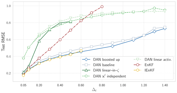
Figure 3 Test RMSEs of DA methods as a function of the update time-step Δ_t in between analyses. See text for details.

To avoid early divergences in the training when Δ_t≫0.05, all the DAN schemes benefited from a modified Eq. (2):

$$\begin{array}{}\text{(23)}& {\mathbf{x}}_k^{\mathrm{a}}={\mathbf{x}}_k^{\mathrm{f}}+\mathit{\alpha }{\mathbf{H}}_k^{⊺}{\mathbf{R}}_k^{-\mathrm{1}}{\mathit{\delta }}_k+{\mathbf{a}}_{\mathit{\theta }}({\mathbf{x}}_k^{\mathrm{f}},{\mathbf{H}}_k^{⊺}{\mathbf{R}}_k^{-\mathrm{1}}{\mathit{\delta }}_k),\end{array}$$

where α is a trainable scalar. Note that this formulation is mathematically equivalent to the original Eq. (2). This is only meant to explicitly enforce the solution ${\mathbf{x}}_k^{\mathrm{a}}={\mathbf{y}}_k$ when H_k=I_x, which guides the training in its first few epochs.

The test RMSEs of those DA methods, over a long DA run, are displayed in Fig. 3 as a function of Δ_t. Note that Δ_t=0.60 is already very significantly nonlinear as it corresponds to the Lyapunov time of L96, i.e. the time horizon beyond which the DA system becomes significantly non-Gaussian.

As expected, the two degraded DAN operators severely underperform the other DA schemes, which leverage non-static priors, with a test RMSE that ranges from 0.38 for Δ_t=0.05 to an asymptotic RMSE below 1 for much larger Δ_t. This is consistent with the findings of Boc24 and mirrors the performance of a 3D-Var with static background covariance matrix.

The EnKF offers a very good performance in the mildly nonlinear regime Δ_t≈0.05 but gradually degrades as Δ_t is increased. Moreover, beyond Δ_t=0.80, the EnKF becomes uninformative and its test RMSE is not reported. As already shown by Sakov et al. (2012), the IEnKF offers significantly better performance, from a marginal improvement over the EnKF at Δ_t=0.05 that gets more and more significant as Δ_t is increased. Note that, beyond Δ_t=0.60, the IEnKF is trickier to stabilise and hence its performance is not reported.

Remarkably, the boosted DAN operator achieves performance very similar to the IEnKF, but can still be learned for much larger Δ_t, and remains informative with still a very significant edge over the static prior methods. Again, this is achieved without the use of an ensemble but of a single forecast state. Moreover, the learned DAN does not explicitly resort to a nonlinear (Gauss-Newton) iterative minimisation, in contrast to the IEnKF. This aspect of such DAN is reminiscent of approaches meant to learn a solver for a variational DA problem (Fablet et al., 2021; Frerix et al., 2021; Lafon et al., 2023; Filoche et al., 2023; Keller and Potthast, 2024). The baseline DAN operator is slightly less performing but follows the same trend. We could have evaluated the methods for even larger Δ_t>1.40; however, Δ_t=1.20 already stands for twice the Lyapunov time, which is equivalent to 6 d in the L96 correspondence.

We suspect that the test RMSEs should primarily be a function of N_iterΔ_t rather than just Δ_t, accounting for the forgetful effect associated to the chaotic dynamics. Hence, to reach the same test RMSEs, N_iter could be roughly chosen inversely proportional to Δ_t. To test this hypothesis, we compare the test RMSE on a large number of trained DANs, varying Δ_t (including for Δ_t≤0.05) and N_iter with results shown in Fig. 4. Leveraging the findings of Appendix B and the use of smaller batches to mitigate the numerical cost, we have chosen for their training, $N_{\mathrm{r}}={\mathrm{2}}^{\mathrm{16}}=\mathrm{65}\mathrm{536}$ and $S_{\mathrm{b}}={\mathrm{2}}^{\mathrm{7}}=\mathrm{128}$. The test RMSEs are shown in Fig. 4. The results corroborate the intuition with the weaker and weaker dependence on N_iter of the performance when Δ_t is increased. Conversely, a much larger N_iter is required when Δ_t gets very small (Δ_t≈0.01).

Figure 4 Test RMSEs of DANs as a function of both Δ_t and N_iter.

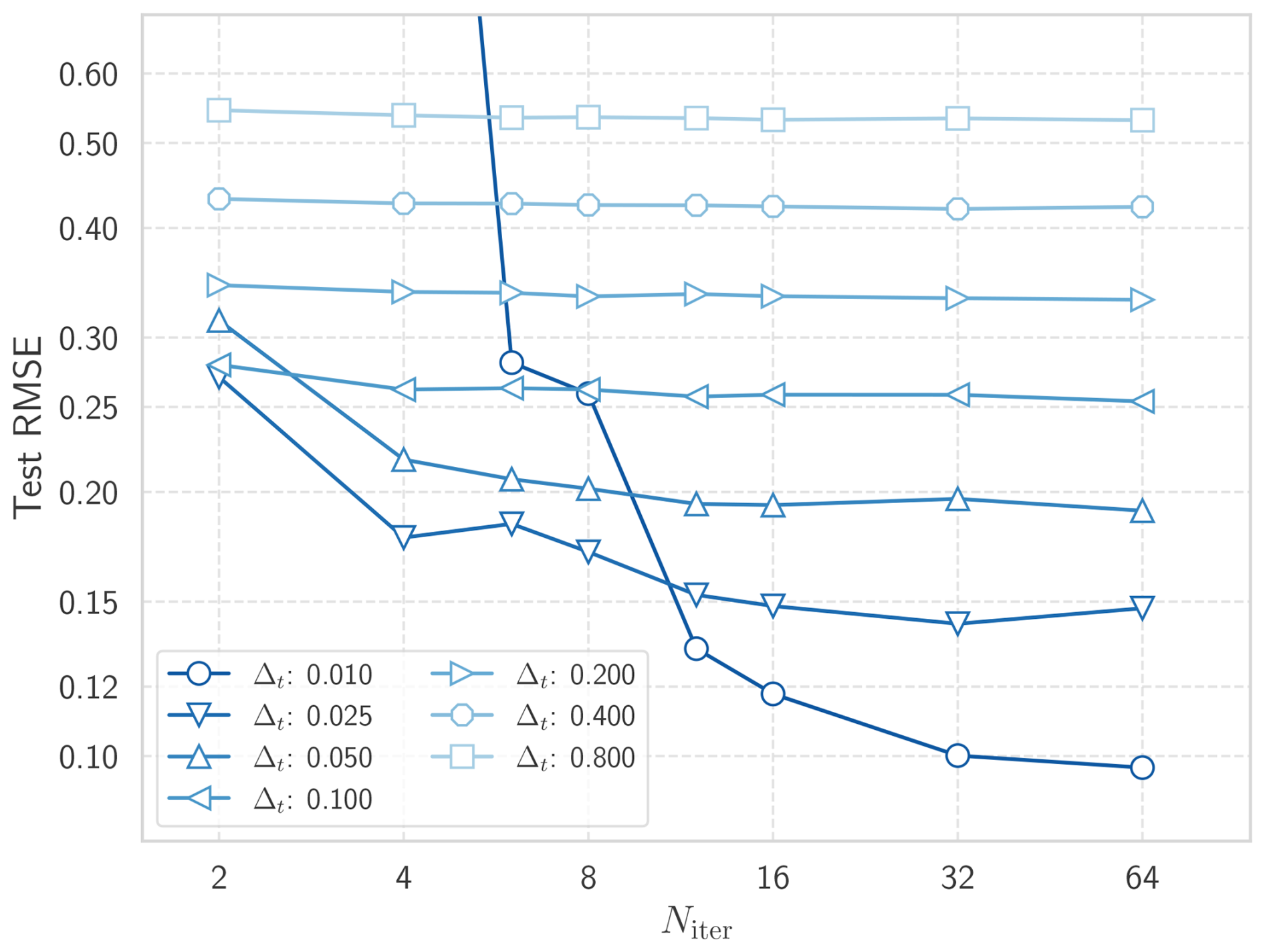
Hence, DAN is numerically more difficult to train when Δ_t<0.05 requiring larger N_iter, which corresponds to quasi-linear regimes where DAN is nonetheless of limited interest.

4.2 Performance as a function of the energy forcing

The forcing F injects and removes energy from the L96 dynamics and feeds their instability. Besides Δ_t, this is another tunable parameter of the nonlinearity of the dynamics. There is a wealth of dynamical phenomenology of the L96 dynamics for a wide range of F (see, e.g., Barone et al., 2025, and references therein). For the range of F we focus on here, instabilities progressively develop in between $\mathrm{1}\lesssim F\lesssim \mathrm{4}$, while chaos fully sets in beyond F≳4 (van Kekem and Sterk, 2018). The number of Lyapunov exponents, and similarly the Kaplan-Yorke dimension, increases monotonically from 4 to about 30 where it saturates (Karimi and Paul, 2010).

We choose the same setup as in the previous experiments and consider the following DA methods:

• A well tuned EnKF with an ensemble of size $N_{\mathrm{e}}=N_{\mathrm{x}}=\mathrm{40}$. Optimal multiplicative inflation is addressed through the finite-size EnKF (Bocquet, 2011; Bocquet et al., 2015), in its Dirac-Jeffreys variant (Bocquet et al., 2015) required to handle the weakly nonlinear regime ($\mathrm{4}\lesssim F\lesssim \mathrm{8}$).

• A well tuned IEnKF with an ensemble of size $N_{\mathrm{e}}=N_{\mathrm{x}}=\mathrm{40}$, whose optimal multiplicative inflation is addressed through the finite-size IEnKF (Bocquet and Sakov, 2012) in its Dirac-Jeffreys variant. This is our hard baseline.

• A (baseline) learned DAN scheme using the neural network and training parameters as defined in Appendix B.

The test RMSEs are displayed in Fig. 5. The IEnKF has a slight edge over the EnKF with larger F with the increasing Kaplan-Yorke dimension. Hence, the DA system does not deviate much from Gaussianity as F increases, rather, it is mainly the magnitude of the instabilities that changes. The DAN achieves a performance in between that of the EnKF and that of the IEnKF, which is patent for large F. Note that it turns out trickier to train DANs for F getting close to 4. There, the dynamics become more and more laminar and exhibit almost periodic waves, with patterns that, although simpler, are very different from those learned in the regimes explored so far.

Figure 5 Test RMSEs of DA methods as a function of the forcing F. See text for details.

4.3 Reasons for the efficiency of data assimilation networks

In the light of the previous numerical results, we discuss the reasons why DAN can be as accurate as the IEnKF, without an ensemble, without any experimental tuning, and even in mildly to strongly nonlinear conditions.

We have already shown in Sect. 3.2 that in the mildly nonlinear regime, i.e. Δ_t≈0.05, the success of DAN mainly resides in its implicit estimation of the map x^f↦P^f(x^f), in line with the results by Sacco et al. (2024) and Sakov (2025), and closely related to the map x^f↦P^a(x^f). As shown in Sect. 3.2.1, this amounts to assume a non-static but Gaussian prior in the analysis: this is equivalent to having $\Vert \mathbf{x}-{\mathbf{x}}^{\mathrm{f}}{\Vert }_{{\left({\mathbf{P}}^{\mathrm{f}}\left({\mathbf{x}}^{\mathrm{f}}\right)\right)}^{-\mathrm{1}}}^{\mathrm{2}}$ as the background term in the analysis cost function. Whether this mechanism is sufficient to ensure the performance of DAN when Δ_t≥0.05 is doubtful.

4.3.1 The linear-in-ζ data assimilation network beyond mild nonlinearity

To address this question, let us assess the linear-in-ζ DAN, see Sect. 3.2, in stronger nonlinear regimes Δ_t≥0.05. We could anticipate that it accounts well for the errors of the day, but that it may not be able to handle stronger nonlinearity/non-Gaussianity, e.g., if Δ_t≫0.05, because of the implied Gaussian prior. It should hence match the EnKF, rather than the IEnKF.

Let us check that hypothesis numerically. The test RMSEs of this specific DAN scheme, which mirrors Eq. (5), are reported in Fig. 3, as the linear-in-ζ DAN. Let us first remark that, in accordance with the claims of Sect. 3.2, it performs as well as the EnKF for Δ_t=0.05. However, as Δ_t increases, its performance significantly degrades compared to the EnKF, not to mention the IEnKF. Even though it relies on an estimate of the x^f↦P^a(x^f) map, its underlying Gaussian assumption penalises it beyond the mildly nonlinear regime, as expected.

4.3.2 Deviation of the data assimilation network prior from Gaussianity

We conclude that the full DAN scheme not only exploits the flow-dependent information represented by the x^f↦P^f(x^f) map, but also learns an effective nonlinear analysis response consistent with a non-Gaussian prior, which is more informative than the Gaussian prior associated to the analysis cost function background term $\Vert \mathbf{x}-{\mathbf{x}}^{\mathrm{f}}{\Vert }_{{\left({\mathbf{P}}^{\mathrm{f}}\left({\mathbf{x}}^{\mathrm{f}}\right)\right)}^{-\mathrm{1}}}^{\mathrm{2}}$. As shown, both abilities are required for DAN to perform so well in the extended range of mildly to strongly nonlinear regimes.

Figure 6 Scaling of the standardised analysis increments of a_θ in the projected innovations, for a large range of Δ_t values.

We investigate the deviation of a_θ from the presumed quasi-linearity in ζ by defining the scalar function

$$\begin{array}{}\text{(24)}& r\left(\mathit{\lambda }\right)={\mathbb{E}}_{\mathbf{x},\mathit{\zeta }}\left[{\displaystyle \frac{∥{\mathbf{P}}^{\mathrm{a}}(\mathbf{x}{)}^{-\mathrm{1}}\left({\mathbf{a}}_{\mathit{\theta }}(\mathbf{x},\mathit{\lambda }\mathit{\zeta })-{\mathbf{a}}_{\mathit{\theta }}(\mathbf{x},\mathbf{0})\right)∥}{∥{\mathbf{P}}^{\mathrm{a}}(\mathbf{x}{)}^{-\mathrm{1}}\left({\mathbf{a}}_{\mathit{\theta }}(\mathbf{x},\mathit{\zeta })-{\mathbf{a}}_{\mathit{\theta }}(\mathbf{x},\mathbf{0})\right)∥}}\right],\end{array}$$

where ∥⋅∥ is the Euclidean norm. It depends on a dimensionless scale parameter λ>0 and measures deviations from the linearity in ζ. In Eq. (24), P^a(x)⁻¹ is meant to standardise the deviations from linearity. Indeed, in the quasi-linear regime, we have

$$\begin{array}{}\text{(25)}& {\mathbf{P}}^{\mathrm{a}}(\mathbf{x}{)}^{-\mathrm{1}}\left({\mathbf{a}}_{\mathit{\theta }}(\mathbf{x},\mathit{\lambda }\mathit{\zeta })-{\mathbf{a}}_{\mathit{\theta }}(\mathbf{x},\mathbf{0})\right)\approx \mathit{\lambda }\mathit{\zeta },\end{array}$$

such that r(λ)≃λ should hold. The ratio r(λ) is estimated using perturbations as in Boc24: x and ζ are sampled from the forecast state x^f and the projected innovations $\mathit{\zeta }={\mathbf{H}}^{⊺}{\mathbf{R}}^{-\mathrm{1}}(\mathbf{y}-{\mathbf{Hx}}^{\mathrm{f}})$ that are obtained from a long trajectory.

The deviation from r(λ)≃λ is demonstrated in Fig. 6 with λ↦r(λ) plotted for several values of Δ_t in the range [0.05,1.5]. These curves should be appreciated knowing the range of values taken by the projected innovations in a long DA run for the selected values of Δ_t which, for each Δ_t, points to the relevant range of λ values to consider and which mainly contributes to the computation of r(λ). This is shown in Fig. 7 in the form of histograms of those values. Given the range of innovation values and the logarithmic scale of Fig. 6, the most relevant part of the scaling behaviour sits in the range $\mathit{\lambda }\in [\mathrm{1},\mathrm{10}]$. In this range of the scaling, as seen in Fig. 6, the more nonlinear the DA run, the steeper λ↦r(λ): the innovation impact is stronger than the one expected in the linear regime, especially for large magnitude innovations.

Figure 7 Histograms of the projected innovations' norm, for a large range of Δ_t values.

5 Discussion and conclusions

In this paper, we have continued to explore the potential of learning sequential DA operators with neural networks for tracking chaotic dynamical systems, following on the initial results and conclusions of Boc24 who built on the concepts of data assimilation networks (DANs) introduced by McCabe and Brown (2021) and Boudier et al. (2023). Assuming the dynamics to be known, the focus is on learning the analysis. Compared to learning the analysis from a dataset of inputs and outputs of DA runs, the training is numerically challenging since the analysis operator is learned through several DA cycles and from trajectories of the dynamics and its observations only.

The resulting DANs are robust, in the sense that they do not require inflation or any other correction and regularisation. They can operate without an ensemble and only use the forecast state as prior information. And yet, they are as accurate as a well tuned EnKF in mildly nonlinear regime, and as accurate as a well tuned IEnKF from mildly to strongly nonlinear conditions.

5.1 Abilities of data assimilation networks

We have previously shown that, to achieve this level of performance, DAN must implicitly learn a map x^f↦P^a(x^f), at least in the mildly nonlinear regime. Its existence is supported by a multiplicative ergodic theorem applied to the entire DA process viewed as a dynamical system. The network must implicitly identify spatial local patterns in x^f in order to internally represent components of P^f(x^f) or P^a(x^f), a property that makes the learned DA method scalable.

In this paper, we further examined the reliance of DANs on the map x^f↦P^a(x^f) by constructing an ad hoc learnable DAN that explicitly incorporates this mapping. For the L96 dynamics, we identified an average characteristic local pattern by leveraging both the invariant distribution of the dynamics and the translational symmetry of the model. We also showed that DAN can learn an effective nonlinear analysis response consistent with non-Gaussian prior information inferred from x^f, and that this nonlinear analysis is necessary for DAN to match the performance of the IEnKF under more stringent nonlinear conditions. In this regime, we demonstrated that implicit or explicit knowledge of the mapping alone is insufficient. Thus, both mechanisms must operate within DAN, paralleling IEnKF's critical reliance on its ensemble for flow-dependent error estimation and on its Gauss-Newton iterative solver to probe departures of the dynamics from linearity.

5.2 Implication for the end-to-end processors in numerical weather prediction

Taken in the context of past DA literature, these results are somewhat surprising. For a long time, it was believed that an ensemble was essential for estimating flow-dependent errors. Moreover, the proper construction of non-Gaussian priors has remained a long-standing challenge, whereas even a simple DAN can rapidly learn an effective nonlinear analysis response consistent with such non-Gaussian information. These findings should inform the (re-)design of future DA algorithms.

These considerations have implications for what DAN-like operators are capable of achieving. For example, recently developed end-to-end atmospheric processors (Allen et al., 2025; Boucher et al., 2025) that ingest observations and predict future observations, implicitly construct their own internal representation of the system and repeatedly compare this latent state to newly assimilated observations. In doing so, they implicitly learn an analysis operator in their latent space. Lean et al. (2025) concluded that their processor, GraphDOP, must be able to learn not only a climatological background but also dynamical priors, a result that may seem surprising given that GraphDOP does not rely on any explicit background information. However, in light of our results, GraphDOP can be interpreted as learning a mapping from the 12 h observational snapshot used as input to the processor to a latent representation that contains information analogous to underlying error covariances. Consequently, it must be able to construct its own background, incorporating advanced error statistics that go beyond a mere climatology. This interpretation is consistent with the diagnostic study of Laloyaux et al. (2025), who applied classical DA tools, including forecast-sensitivity observation-impact diagnostics, to GraphDOP. Their results suggest that GraphDOP learns physically meaningful spatial relationships and latent Earth-system representations from observations. While this does not show that GraphDOP explicitly estimates a forecast-error covariance, it supports the broader view that end-to-end observation-driven processors can develop DA-like internal representations without being supplied with an explicit background state.

This challenges the view that the accuracy of such end-to-end processors is fundamentally limited by the absence of a background (such as a forecast ensemble or climatological information) in their inputs. While an explicit background representation would certainly provide additional information, the extent of the achievable performance gains remains a subtler question.

5.3 Ensembles, uncertainty quantification, and multiplicative ergodic theorem

Our results show that, in the perfect-model filtering setting considered here, an explicit forecast ensemble is not strictly required for a learned analysis operator to extract the flow-dependent information needed to achieve EnKF-like point-estimation accuracy. This conclusion should not be interpreted as a dismissal of ensemble representations in general. Ensembles remain essential for probabilistic forecasting, uncertainty quantification, the diagnosis of model and observation errors, smoothing, risk-sensitive applications, and regimes in which the posterior distribution is strongly non-Gaussian or multi-modal.

Moreover, the deterministic analysis operator a_θ could itself be used as a building block for ensemble generation. For instance, applying a_θ to perturbed innovations would produce a set of analysis states, in a way that is consistent with the local, innovation-dependent interpretation used in, e.g., Appendix I to obtain the linear regression approximation of a_θ with respect to ζ. Such an analysis ensemble could then be propagated by the forecast model to estimate forecast uncertainty. We have not pursued this probabilistic use of DAN in the present study, since our focus was on point-estimation accuracy, but it represents a natural direction for future work.

At a more theoretical level, the success of DAN may be facilitated by the existence, in the present setting, of a sufficiently regular and local dependence of the relevant flow-dependent analysis correction on the forecast state. This should not be taken for granted in general. For example, the multiplicative ergodic theorem ensures that covariant Lyapunov subspaces are defined as measurable functions of the state, for almost every state on the attractor, but it does not guarantee that this state-to-Oseledets-splitting map is continuous, local, or easily learnable from finite data. Other applications beyond DA, such as learning covariant Lyapunov vectors directly from the state, may therefore involve maps with poorer regularity or locality, making them substantially more difficult to learn and possibly less scalable. This question is left for future work.

Appendix A: Neural network architecture

As described in Boc24, we choose for a_θ a basic residual convolutional neural network (CNN) architecture. A schematic of the CNN architecture is displayed in Fig. A1. It begins with an initial convolution that takes N_e+1 channels as inputs and, with N_f filters, outputs N_f channels. This initial layer is followed by N_b residual blocks. Each one of these blocks is a succession of N_sb sub-blocks. Each subblock is made of: (i) a convolutional layer with N_f channels as inputs, which has N_f filters and a kernel size f_v for each of its filter, (ii) a batch normalisation layer, and (iii) an activation function chosen to be Mish (Misra, 2019). The CNN ends with a final convolutional layer that takes N_f channels as inputs and, with N_e filters, outputs N_e channels. The kernel size of the initial and final channels is f_v. Hence, the internal state of the CNN consists of N_f copies of the latent space which we simply choose to be isomorphic to the state space ${\mathbb{R}}^{N_{\mathrm{x}}}$. In this paper, only N_e=1 is used. For all experiments, the internal architecture parameter values are N_b=5, N_sb=5, f_v=5.

Figure A1 Architecture of the residual convolutional network where, for this specific illustration, N_b=2, N_sb=3. ${\text{conv}}_{N_{\mathrm{1}},N_{\mathrm{2}},f}$ is a generic one-dimensional convolutional layer of dimension N₁, with N₂ filters of kernel size f. See text for more details.

Appendix B: Sensitivity to the batch size, the size of the datasets, and the backpropagation truncation

The key parameters in the design of a_θ and especially in its training are:

• the number of channels/filters N_f processed by the convolutional neural network (see Appendix A). This essentially gives away the complexity of the neural network, how many features it can identify and process.

• the number of trajectory N_r processed in parallel. The larger N_r, the more DA runs the neural network can learn from and be made robust against. 10 % of these are reserved for validation.

• the number of cycles N_iter through which the gradient is computed. This corresponds to the limit imposed by the truncated backpropagation through time. The larger N_iter≪N_c, the better the information transmission from one cycle to the next should be learned, but the more costly and less accurate the gradients.

• the size of the batch S_b. Hence, the number of steps in each epoch is about $N_{\mathrm{r}}/S_{\mathrm{b}}$ (training and validation).

The training parameters N_r, N_iter, and to a lesser extend N_c are the key dimensions specifying how the data are fed to the training schedule as schematised in Fig. B1.

Figure B1 This schematic describes how data are fed to the training scheme; it must be read from left to right (time arrow). For instance, in epoch 2, N_iter-long segments of N_r trajectories feed the training algorithm. The segments are organised and provided in batches of size S_b.

The dependence of the performance of a_θ on those parameters was studied in Boc24. The values N_iter=16, N_r=2¹⁸, S_b=2048 were chosen for the a_θ hyperparameters of the reference setup, as a compromise between training speed and accuracy of the resulting a_θ. However, the dependence on N_iter and S_b was barely reported and discussed, so that we focus on them in what follows.

Using the reference DA setup, we compute the test RMSE of the DAN schemes as a function of the truncation number N_iter. The results are shown in Fig. B2. As expected, N_iter≤5 prevents DAN from learning an efficient prior that relies on the errors of the day. It is however remarkable that the improvement in the test RMSE as N_iter increases is noticeable up to about N_iter≃40, which corresponds to about 6 times the doubling time of the L96 model in the reference setup.

Figure B2 Test RMSE of DAN as a function of the truncation cycles number $N_{\text{iter}}=\mathrm{1},\mathrm{\dots },\mathrm{40}$ in the truncated backpropagation. For each value of N_c, an ensemble of 5 a_θ operators is learned. Plus and minus one standard deviation of the RMSE are displayed as shades around the RMSE curve.

We have also experimented with the batch size S_b much more thoroughly than in Boc24. We found that using smaller batches is beneficial to the performance of the trained a_θ. This may also enable reducing the number of trajectories N_r in the dataset. Nonetheless, we empirically found that the number of steps, i.e. $\sim N_{\mathrm{r}}/S_{\mathrm{b}}$ in each epoch still needs to remain large to achieve high accuracy. Experimenting, we learned a large set of a_θ operators with N_r in the range 2¹⁰–2¹⁸, while S_b is chosen in the range 2³–2⁸. The corresponding test RMSEs are plotted as a function of either S_b, as shown in Fig. B3a, or N_r as shown in Fig. B3b.

Figure B3 Test RMSEs of DAN as a function of the batch size S_b for a selection of N_r values (panel a) and as a function of the number of dataset trajectories N_r for a selection of S_b values (panel b). For each pair (S_b,N_r), an ensemble of 3 a_θ operators is learned, from which error bars (plus or minus the standard deviation) are estimated and added to the curve plots.

For this specific configuration a scaling law can be numerically estimated. The following Ansatz is assumed:

$$\begin{array}{}\text{(B1)}& {\text{RMSE}}^{\mathrm{1}/\mathit{\gamma }}=f\left({\displaystyle \frac{N_{\mathrm{r}}^{\mathit{\alpha }}}{S_{\mathrm{b}}^{\mathit{\beta }}}}\right),\end{array}$$

where f is a polynomial of order 2. This Ansatz (3 polynomial coefficients and 3 exponents) is fitted to the test RMSE results. The fit relevance can be visualised through the plot of f^γ in Fig. B4. The fitted exponents are γ=1.435, α=0.103, and β=0.060. What really matters is the ratio $\mathit{\rho }=\mathit{\beta }/\mathit{\alpha }=\mathrm{0.58}$, since the test RMSE turns out to show a strong dependence on $N_{\mathrm{r}}/S_{\mathrm{b}}^{\mathit{\rho }}$.

Figure B4 Checking the relevance of the functional regression by plotting the fit function f^γ with respect to $N_{\mathrm{r}}^{\mathit{\alpha }}/S_{\mathrm{b}}^{\mathit{\beta }}$ (curve), and of the test RMSE results (dots).

In practice, the interest of using smaller batches S_b and hence smaller N_r must be weighted against the overheads created by the dataset pipeline but also by the transfer of the batches from RAM to VRAM. It is however possible to run several training experiments in parallel over the same GPU with smaller batches. Hence, the efficiency of using mini-batches is very dependent on the accelerator device(s) and the type of experiment to conduct. Note that, when training a_θ on much higher dimensional systems, relying on mini-batches may become mandatory so as to fit into VRAM.

Finally, the scaling law Eq. (B1) can be leveraged to reduce both N_r and S_b and still be able to extrapolate to values yielding better test RMSEs, using the dependence on $N_{\mathrm{r}}/S_{\mathrm{b}}^{\mathit{\rho }}$. This scaling could nonetheless change with a different DA setup.

Appendix C: Neural network implementation of the effective x^f↦P^a(x^f) map

Here, we detail how to build the linear-in-ζ DAN meant to enforce Eq. (9) in Sect. 3.2. Implementing the map $({\mathbf{x}}^{\mathrm{f}},\mathit{\zeta })\mapsto {\mathbf{P}}^{\mathrm{a}}\left({\mathbf{x}}^{\mathrm{f}}\right)\cdot \mathit{\zeta }$ as a neural network is non-trivial if we wish to make it scalable. First, P^a(x^f) is symmetric positive definite; to enforce such constraint, the usual most efficient approach is to write: ${\mathbf{P}}^{\mathrm{a}}\left({\mathbf{x}}^{\mathrm{f}}\right)={\mathbf{X}}^{\mathrm{a}}\left({\mathbf{x}}^{\mathrm{f}}\right){\mathbf{X}}^{\mathrm{a}}({\mathbf{x}}^{\mathrm{f}}{)}^{⊺}$, where X^a(x^f) is a matrix of anomalies which may be easier to interpret than P^a(x^f). The first difficulty towards scalability is the fact that P^a(x^f), or X^a(x^f), is of size N_x×N_x, which is considered non-scalable. However, if P^a(x^f) can be approximated as low-rank, then ${\mathbf{P}}^{\mathrm{a}}\left({\mathbf{x}}^{\mathrm{f}}\right)\approx {\mathbf{X}}^{\mathrm{a}}\left({\mathbf{x}}^{\mathrm{f}}\right){\mathbf{X}}^{\mathrm{a}}({\mathbf{x}}^{\mathrm{f}}{)}^{⊺}$ with X^a(x^f) of size N_x×N_r, with N_r remaining small enough when N_x is increased. Unfortunately, P^a(x^f) should not realistically be considered low-rank. However, one can exploit the locality of the covariances and write ${\mathbf{P}}^{\mathrm{a}}\left({\mathbf{x}}^{\mathrm{f}}\right)\approx \mathit{\rho }\circ \left({\mathbf{X}}^{\mathrm{a}}\left({\mathbf{x}}^{\mathrm{f}}\right){\mathbf{X}}^{\mathrm{a}}({\mathbf{x}}^{\mathrm{f}}{)}^{⊺}\right)$, where ρ is the localisation correlation matrix and ∘ is the Schur/Hadamard product. In addition to making P^a(x^f) full rank in spite of a manageable number of parameters in X^a(x^f), it also tapers spurious correlations that could be learned in the course of the training. Indeed, the implementation of the localisation significantly accelerates the training. This is reminiscent of the proposal by Bocquet and Farchi (2019) to estimate X^a through a loss involving a Schur product with ρ.

Furthermore, given ${\mathbf{P}}^{\mathrm{a}}=\mathit{\rho }\circ \left({\mathbf{X}}^{\mathrm{a}}{\left({\mathbf{X}}^{\mathrm{a}}\right)}^{⊺}\right)$ and the projected innovation ζ, the implementation of such mapping can be efficiently coded using (see, e.g., Desroziers et al., 2014)

$$\begin{array}{}\text{(C1)}& {\mathbf{P}}^{\mathrm{a}}\cdot \mathit{\zeta }=\mathit{\rho }\circ \left({\mathbf{X}}^{\mathrm{a}}{\left({\mathbf{X}}^{\mathrm{a}}\right)}^{⊺}\right)\cdot \mathit{\zeta }=\sum _{l=\mathrm{1}}^{N_{\mathrm{r}}}{\mathbf{X}}_l^{\mathrm{a}}\circ \left(\mathit{\rho }\cdot \left({\mathbf{X}}_l^{\mathrm{a}}\circ \mathit{\zeta }\right)\right),\end{array}$$

where the ${\mathbf{X}}_l^{\mathrm{a}}$ are the columns of X^a, and ⋅ denotes the usual matrix/vector multiplication. The matrix multiplication by the localisation matrix ρ is scalable since ρ is assumed to be a banded matrix. With L96 in mind, i.e. in a one-dimensional context, with a localisation matrix support of (band-)width N_l, the numerical complexity of P^a⋅ζ is N_rN_x(2+N_l).

If localisation is not useful and P^a(x^f) is low-rank, then it is easy to implement ${\mathbf{P}}^{\mathrm{a}}\cdot \mathit{\zeta }={\mathbf{X}}^{\mathrm{a}}\cdot \left({\left({\mathbf{X}}^{\mathrm{a}}\right)}^{⊺}\cdot \mathit{\zeta }\right)$, which is reminiscent of the very popular machine learning attention mechanism. The numerical complexity is then 2N_rN_x.

An alternative linear-in-ζ DAN is to implement an hypernetwork which would map x^f to a set of weights and biases of a linear neural network that would then be applied to ζ. Naively, the number of weights and biases could scale like $N_{\mathrm{x}}^{\mathrm{2}}$. However, we can instead map x^f to weights and biases of a sequence of convolutional neural networks that we later apply to ζ. Yet, we did not test this more sophisticated construction since the former approach is scalable and successful.

Appendix D: Stein lemma for ∇_ζa_θ(x,ζ)

Here, we offer a proof of the Stein lemma in the degenerate case where the Gaussian density is singular within the embedding space. This is useful with sparse observations resulting in ζ confined within a subspace of E_x. This subsumes the full-rank case. Let us assume that ρ is the pdf defined over E_x of the Gaussian random vector ζ, whose mean is $\stackrel{\mathrm{‾}}{\mathit{\zeta }}$ and whose covariance matrix is Σ_ρ which is assumed positive semi-definite. Hence, the support of ζ may be singular in E_x. That is why we resort to the singular value decomposition ${\mathbf{\Sigma }}_{\mathit{\rho }}=\mathbf{U}{\mathbf{\Sigma }}_{\mathit{\lambda }}{\mathbf{U}}^{⊺}$, where U is an orthonormal (though not necessarily orthogonal) matrix such that ${\mathbf{U}}^{⊺}\mathbf{U}={\mathbf{I}}_{\mathrm{x}}$, and Σ_λ is a positive definite diagonal matrix of rank lower or equal to N_x. We can parametrise the random vector ζ by

$$\begin{array}{}\text{(D1)}& \mathit{\zeta }\left(\mathit{\omega }\right)=\stackrel{\mathrm{‾}}{\mathit{\zeta }}+\mathbf{U}\mathit{\omega },\end{array}$$

where the random vector ω has $\mathit{\lambda }\left(\mathit{\omega }\right)=n(\mathbf{0},{\mathbf{\Sigma }}_{\mathit{\lambda }})$ for Gaussian pdf. Then, denoting $f\left(\mathit{\zeta }\right)\stackrel{\Delta }{=}{\mathbf{a}}_{\mathit{\theta }}(\mathbf{x},\mathit{\zeta })$ for brevity, we have

$$\begin{array}{ll}{\displaystyle }\text{Cov}& {}_{\mathit{\zeta }\sim \mathit{\rho }}\left[\mathit{\zeta },f\left(\mathit{\zeta }\right)\right]\\ \text{(D2a)}& {\displaystyle }& {\displaystyle }={\text{Cov}}_{\mathit{\omega }\sim \mathit{\lambda }}\left[\mathit{\zeta }\left(\mathit{\omega }\right),f\left(\mathit{\zeta }\right(\mathit{\omega }\left)\right)\right]\text{(D2b)}& {\displaystyle }& {\displaystyle }=\int \mathrm{d}\mathit{\omega }\mathit{\lambda }\left(\mathit{\omega }\right)\left(\mathit{\zeta }\right(\mathit{\omega })-\stackrel{\mathrm{‾}}{\mathit{\zeta }})\otimes \left(f\left(\mathit{\zeta }\right(\mathit{\omega }\left)\right)-f\left(\stackrel{\mathrm{‾}}{\mathit{\zeta }}\right)\right)\text{(D2c)}& {\displaystyle }& {\displaystyle }=\int \mathrm{d}\mathit{\omega }\mathit{\lambda }\left(\mathit{\omega }\right)\left(\mathbf{U}\mathit{\omega }\right)\otimes f\left(\mathit{\zeta }\right(\mathit{\omega }\left)\right)\text{(D2d)}& {\displaystyle }& {\displaystyle }=\mathbf{U}{\mathbf{\Sigma }}_{\mathit{\lambda }}\int \mathrm{d}\mathit{\omega }\mathit{\lambda }\left(\mathit{\omega }\right)\left({\mathbf{\Sigma }}_{\mathit{\lambda }}^{-\mathrm{1}}\mathit{\omega }\right)\otimes f\left(\mathit{\zeta }\right(\mathit{\omega }\left)\right)\text{(D2e)}& {\displaystyle }& {\displaystyle }=-\mathbf{U}{\mathbf{\Sigma }}_{\mathit{\lambda }}\int \mathrm{d}\mathit{\omega }\mathit{\lambda }\left(\mathit{\omega }\right){\mathrm{\nabla }}_{\mathit{\omega }}\ln \mathit{\lambda }\left(\mathit{\omega }\right)\otimes f\left(\mathit{\zeta }\right(\mathit{\omega }\left)\right)\text{(D2f)}& {\displaystyle }& {\displaystyle }=-\mathbf{U}{\mathbf{\Sigma }}_{\mathit{\lambda }}\int \mathrm{d}\mathit{\omega }{\mathrm{\nabla }}_{\mathit{\omega }}\mathit{\lambda }\left(\mathit{\omega }\right)\otimes f\left(\mathit{\zeta }\right(\mathit{\omega }\left)\right)\text{(D2g)}& {\displaystyle }& {\displaystyle }=\mathbf{U}{\mathbf{\Sigma }}_{\mathit{\lambda }}\int \mathrm{d}\mathit{\omega }\mathit{\lambda }\left(\mathit{\omega }\right){\mathrm{\nabla }}_{\mathit{\omega }}\left(f\left(\mathit{\zeta }\right(\mathit{\omega }\left)\right)\right)\text{(D2h)}& {\displaystyle }& {\displaystyle }=\mathbf{U}{\mathbf{\Sigma }}_{\mathit{\lambda }}{\mathbf{U}}^{⊺}\int \mathrm{d}\mathit{\omega }\mathit{\lambda }\left(\mathit{\omega }\right)\left({\mathrm{\nabla }}_{\mathit{\zeta }}f\right)\left(\mathit{\zeta }\right(\mathit{\omega }\left)\right)\text{(D2i)}& {\displaystyle }& {\displaystyle }={\mathbf{\Sigma }}_{\mathit{\rho }}{\mathbb{E}}_{\mathit{\omega }\sim \mathit{\lambda }}\left[\left({\mathrm{\nabla }}_{\mathit{\zeta }}f\right)\left(\mathit{\zeta }\right(\mathit{\omega }\left)\right)\right]\text{(D2j)}& {\displaystyle }& {\displaystyle }={\mathbf{\Sigma }}_{\mathit{\rho }}{\mathbb{E}}_{\mathit{\zeta }\sim \mathit{\rho }}\left[{\mathrm{\nabla }}_{\mathit{\zeta }}f\right].\end{array}$$

Hence, we conclude:

$$\begin{array}{}\text{(D3)}& {\mathbb{E}}_{\mathit{\zeta }\sim \mathit{\rho }}\left[{\mathrm{\nabla }}_{\mathit{\zeta }}f\right]={\mathbf{\Sigma }}_{\mathit{\rho }}^{†}{\text{Cov}}_{\mathit{\zeta }\sim \mathit{\rho }}\left[\mathit{\zeta },f\left(\mathit{\zeta }\right)\right],\end{array}$$

where $(\cdot {)}^{†}$ is the Moore-Penrose inverse operator, which comes with the regularisation choice to taper 𝔼_ζ∼ρ[∇_ζf] outside of the range of ζ. Applied to $f\left(\mathit{\zeta }\right)={\mathbf{a}}_{\mathit{\theta }}(\mathbf{x},\mathit{\zeta })$, this yields:

$$\begin{array}{}\text{(D4a)}& {\mathbb{E}}_{\mathit{\zeta }\sim \mathit{\rho }}\left[{\mathrm{\nabla }}_{\mathit{\zeta }}{\mathbf{a}}_{\mathit{\theta }}(\mathbf{x},\mathit{\zeta })\right]={\mathbf{\Sigma }}_{\mathit{\rho }}^{†}{\text{Cov}}_{\mathit{\zeta }\sim \mathit{\rho }}\left[\mathit{\zeta },{\mathbf{a}}_{\mathit{\theta }}(\mathbf{x},\mathit{\zeta })\right],\end{array}$$

which, if Σ_ρ is full rank, can be written (usual Stein lemma)

$$\begin{array}{}\text{(D4b)}& {\mathbb{E}}_{\mathit{\zeta }\sim \mathit{\rho }}\left[{\mathrm{\nabla }}_{\mathit{\zeta }}{\mathbf{a}}_{\mathit{\theta }}(\mathbf{x},\mathit{\zeta })\right]={\mathbf{\Sigma }}_{\mathit{\rho }}^{-\mathrm{1}}{\text{Cov}}_{\mathit{\zeta }\sim \mathit{\rho }}\left[\mathit{\zeta },{\mathbf{a}}_{\mathit{\theta }}(\mathbf{x},\mathit{\zeta })\right].\end{array}$$

Appendix E: Comparing the empirical and theoretical mean marginal gains

In Sect. 3.3, we showed that the theoretical mean marginal gain $\stackrel{\mathrm{‾}}{\mathbf{\Gamma }}$ is expected to be a good approximation of the less simple theoretical mean

$$\begin{array}{}\text{(E1)}& \stackrel{\mathrm{̃}}{\mathbf{\Gamma }}=\int \mathrm{d}\mathbf{x}\mathrm{d}\mathit{\zeta }\mathit{\pi }\left(\mathbf{x}\right)\mathit{\rho }\left(\mathit{\zeta }\right){\mathrm{\nabla }}_{\mathbf{x}}{\mathrm{\nabla }}_{\mathit{\zeta }}{\mathbf{a}}_{\mathit{\theta }}(\mathbf{x},\mathit{\zeta }).\end{array}$$

The latter can now be related to the empirical mean of Γ over a long DA run, denoted $\widehat{\mathbf{\Gamma }}$, and which is obtained from numerical experiments. This is meant to ensure that a pattern emerging from our approximation of $\stackrel{\mathrm{‾}}{\mathbf{\Gamma }}$, is nonetheless consistent with those learned through a_θ over the training DA dataset. Hence, given a long trajectory of true states and projected innovations ${\mathcal{T}}_{\mathbf{x},\mathit{\zeta }}=\mathit{\left\{}\right({\mathbf{x}}_k^{\mathrm{t}},{\mathit{\zeta }}_k){\mathit{\}}}_{k=\mathrm{1},\mathrm{\dots },K}\subset ({\mathbf{E}}_{\mathrm{x}}\times {\mathbf{E}}_{\mathrm{x}}{)}^K$, the empirical sensitivity associated to $\stackrel{\mathrm{̃}}{\mathbf{\Gamma }}$, and hence $\stackrel{\mathrm{‾}}{\mathbf{\Gamma }}$, should be

$$\begin{array}{}\text{(E2a)}& {\displaystyle }\widehat{\mathbf{\Gamma }}& {\displaystyle }\stackrel{\Delta }{=}\langle \mathbf{\Gamma }({\mathbf{x}}^{\mathrm{t}},\mathit{\zeta }){\rangle }_{({\mathbf{x}}^{\mathrm{t}},\mathit{\zeta })\in {\mathcal{T}}_{\mathbf{x},\mathit{\zeta }}}\text{(E2b)}& {\displaystyle }& {\displaystyle }\underset{K\to \mathrm{\infty }}{=}\int \mathrm{d}{\mathbf{x}}^{\mathrm{t}}\mathrm{d}\mathit{\zeta }p({\mathbf{x}}^{\mathrm{t}},\mathit{\zeta })\mathbf{\Gamma }({\mathbf{x}}^{\mathrm{t}},\mathit{\zeta }),\end{array}$$

where p(x^t,ζ) is the joint distribution of x^t and ζ. However, ζ_k not only depends on ${\mathbf{x}}_k^{\mathrm{t}}$ but also on the forecast ${\mathbf{x}}_k^{\mathrm{f}}$, so that:

$$\begin{array}{}\text{(E3)}& \widehat{\mathbf{\Gamma }}=\int \mathrm{d}{\mathbf{x}}^{\mathrm{t}}\mathrm{d}{\mathbf{x}}^{\mathrm{f}}\mathrm{d}\mathit{\zeta }p({\mathbf{x}}^{\mathrm{t}},{\mathbf{x}}^{\mathrm{f}},\mathit{\zeta })\mathbf{\Gamma }({\mathbf{x}}^{\mathrm{t}},\mathit{\zeta }),\end{array}$$

or, introducing the forecast error ${\mathbf{e}}^{\mathrm{f}}\stackrel{\Delta }{=}{\mathbf{x}}^{\mathrm{f}}-{\mathbf{x}}^{\mathrm{t}}$,

$$\begin{array}{}\text{(E4)}& \widehat{\mathbf{\Gamma }}=\int \mathrm{d}{\mathbf{x}}^{\mathrm{t}}\mathrm{d}{\mathbf{e}}^{\mathrm{f}}\mathrm{d}\mathit{\zeta }p({\mathbf{x}}^{\mathrm{t}},{\mathbf{e}}^{\mathrm{f}},\mathit{\zeta })\mathbf{\Gamma }({\mathbf{x}}^{\mathrm{t}}+{\mathbf{e}}^{\mathrm{f}},\mathit{\zeta }).\end{array}$$

By marginalising over x^t, we have

$$\begin{array}{}\text{(E5a)}& {\displaystyle }\widehat{\mathbf{\Gamma }}& {\displaystyle }=\int \mathrm{d}{\mathbf{x}}^{\mathrm{t}}\mathit{\pi }\left({\mathbf{x}}^{\mathrm{t}}\right)\int \mathrm{d}{\mathbf{e}}^{\mathrm{f}}\mathrm{d}\mathit{\zeta }p({\mathbf{e}}^{\mathrm{f}},\mathit{\zeta }|{\mathbf{x}}^{\mathrm{t}}\left)\mathbf{\Gamma }\right({\mathbf{x}}^{\mathrm{t}}+{\mathbf{e}}^{\mathrm{f}},\mathit{\zeta })\text{(E5b)}& {\displaystyle }& {\displaystyle }=\int \mathrm{d}{\mathbf{x}}^{\mathrm{t}}\mathit{\pi }\left({\mathbf{x}}^{\mathrm{t}}\right)\int \mathrm{d}{\mathbf{e}}^{\mathrm{f}}\mathrm{d}\mathit{\zeta }p\left(\mathit{\zeta }\right|{\mathbf{e}}^{\mathrm{f}}\left)p\right({\mathbf{e}}^{\mathrm{f}}\left|{\mathbf{x}}^{\mathrm{t}}\right)\mathbf{\Gamma }({\mathbf{x}}^{\mathrm{t}}+{\mathbf{e}}^{\mathrm{f}},\mathit{\zeta })\text{(E5c)}& {\displaystyle }& {\displaystyle }\approx \int \mathrm{d}{\mathbf{x}}^{\mathrm{t}}\mathit{\pi }\left({\mathbf{x}}^{\mathrm{t}}\right)\int \mathrm{d}\mathit{\zeta }\left[p\right(\mathit{\zeta }\left|{\mathbf{e}}^{\mathrm{f}}\right)\mathbf{\Gamma }({\mathbf{x}}^{\mathrm{t}}+{\mathbf{e}}^{\mathrm{f}},\mathit{\zeta }){]}_{{\mathbf{e}}^{\mathrm{f}}=\mathbf{0}}\text{(E5d)}& {\displaystyle }& {\displaystyle }=\int \mathrm{d}{\mathbf{x}}^{\mathrm{t}}\mathit{\pi }\left({\mathbf{x}}^{\mathrm{t}}\right)\int \mathrm{d}\mathit{\zeta }\mathit{\rho }\left(\mathit{\zeta }\right)\mathbf{\Gamma }({\mathbf{x}}^{\mathrm{t}},\mathit{\zeta })=\stackrel{\mathrm{̃}}{\mathbf{\Gamma }}.\end{array}$$

From Eq. (E5a) to Eq. (E5b), we use $p({\mathbf{e}}^{\mathrm{f}},\mathit{\zeta }|{\mathbf{x}}^{\mathrm{t}})=p(\mathit{\zeta }\left|{\mathbf{e}}^{\mathrm{f}}\right)p\left({\mathbf{e}}^{\mathrm{f}}\right|{\mathbf{x}}^{\mathrm{t}})$ since the full dependence of ζ on x^t is in e^f. From Eq. (E5b) to Eq. (E5c), we assume that the forecast error norm is small compared to the norm of x^t, which should indeed be the case in the weak assimilation regime. From Eq. (E5c) to Eq. (E5d), we approximate $p\left(\mathit{\zeta }\right|{\mathbf{e}}^{\mathrm{f}}=\mathbf{0})$ by the marginal ρ(ζ). This points to the (reasonable) approximations made when identifying $\stackrel{\mathrm{̃}}{\mathbf{\Gamma }}$, Eq. (E1), with the empirical marginal gain $\widehat{\mathbf{\Gamma }}$, $\langle \mathbf{\Gamma }(\mathbf{x},\mathit{\zeta }){\rangle }_{(\mathbf{x},\mathit{\zeta })\in {\mathcal{T}}_{\mathbf{x},\mathit{\zeta }}}$, emerging from a long DA run.

Moreover, a formal expression for ρ(ζ|e^f) which appeared in the previous derivation is

$$\begin{array}{ll}{\displaystyle }p\left(\mathit{\zeta }\right|{\mathbf{e}}^{\mathrm{f}})& {\displaystyle }=\int \mathrm{d}\mathit{\epsilon }\mathrm{d}\mathbf{H}\mathrm{d}\mathbf{R}p(\mathit{\epsilon },\mathbf{H},\mathbf{R}|{\mathbf{e}}^{\mathrm{f}})\\ \text{(E6)}& {\displaystyle }& {\displaystyle }\times \mathit{\delta }(\mathit{\zeta }-{\mathbf{H}}^{⊺}{\mathbf{R}}^{-\mathrm{1}}(\mathit{\epsilon }-{\mathbf{He}}^{\mathrm{f}}\left)\right),\end{array}$$

where $p(\mathit{\epsilon },\mathbf{H},\mathbf{R}|{\mathbf{e}}^{\mathrm{f}})$ is the pdf of the joint distribution for the observation error ε, the observation operator H, and the observation error covariance matrix R, given the forecast error e^f. Marginalising over e^f, we obtain

$$\begin{array}{ll}\text{(E7a)}& {\displaystyle }\mathit{\rho }\left(\mathit{\zeta }\right)& {\displaystyle }=\int \mathrm{d}{\mathbf{e}}^{\mathrm{f}}p\left(\mathit{\zeta }\right|{\mathbf{e}}^{\mathrm{f}}\left)p\right({\mathbf{e}}^{\mathrm{f}}){\displaystyle }& {\displaystyle }=\int \mathrm{d}{\mathbf{e}}^{\mathrm{f}}\mathrm{d}\mathit{\epsilon }\mathrm{d}\mathbf{H}\mathrm{d}\mathbf{R}p({\mathbf{e}}^{\mathrm{f}},\mathit{\epsilon },\mathbf{H},\mathbf{R})\\ \text{(E7b)}& {\displaystyle }& {\displaystyle }\times \mathit{\delta }(\mathit{\zeta }-{\mathbf{H}}^{⊺}{\mathbf{R}}^{-\mathrm{1}}(\mathit{\epsilon }-{\mathbf{He}}^{\mathrm{f}}\left)\right).\end{array}$$

This expression is helpful to formally investigate the symmetries of the distribution of ζ, for which Eq. (18) applies.

Appendix F: Proof of the equivariance of the marginal gain tensor

We wish to prove the equivariance of the marginal gain tensor, i.e. that for all x and ζ, $\mathbf{\Gamma }(g\circ \mathbf{x},g\circ \mathit{\zeta })=g\otimes g^{⊺}\otimes g^{⊺}\circ \mathbf{\Gamma }(\mathbf{x},\mathit{\zeta })$, under the action of an isometry g∈𝒢. The action of g on either state vector x or ζ is represented by an orthogonal matrix G: $g\circ \mathbf{x}=\mathbf{Gx}$, $g\circ \mathit{\zeta }=\mathbf{G}\mathit{\zeta }$.

We say that g preserves the fibres (preimages) of ℋ_k if, for all x, x^′ such that ${\mathcal{H}}_k\left(\mathbf{x}\right)={\mathcal{H}}_k\left({\mathbf{x}}^{\prime }\right)$ one has ${\mathcal{H}}_k(g\circ \mathbf{x})={\mathcal{H}}_k(g\circ {\mathbf{x}}^{\prime })$. An isometry g_y defined over the observation space of ℋ_k can then be associated to such g through $g_{\mathrm{y}}\circ {\mathcal{H}}_k(g^{⊺}\circ (\cdot \left)\right)={\mathcal{H}}_k(\cdot )$. The action of such induced isometry g_y is represented by the orthogonal matrix G_y: $g_{\mathrm{y}}\circ \mathbf{y}={\mathbf{G}}_{\mathrm{y}}\mathbf{y}$. Because G and G_y are orthogonal, one has ${\mathbf{G}}^{-\mathrm{1}}={\mathbf{G}}^{⊺}$ and ${\mathbf{G}}_{\mathrm{y}}^{-\mathrm{1}}={\mathbf{G}}_{\mathrm{y}}^{⊺}$.

With these definitions in hand, we consider a maximal group of isometries 𝒢 defined over the state space such that

• 𝒢 preserves the fibres of all ℋ_k, inducing a group of isometries 𝒢_y (possibly for each k). 𝒢_y is isomorphic to 𝒢,

• the associated 𝒢_y satisfies ${\mathbf{G}}_{\mathrm{y}}{\mathbf{R}}_k{\mathbf{G}}_{\mathrm{y}}^{⊺}={\mathbf{R}}_k$, which accounts for any heteroscedasticity of the observation error statistics,

• 𝒢 commutes with the autonomous dynamics, i.e. $\mathbf{G}\mathcal{M}\left({\mathbf{G}}^{⊺}\right(\cdot \left)\right)=\mathcal{M}(\cdot )$.

A consequence of the equivariance with respect to ℋ_k, i.e. ${\mathbf{G}}_{\mathrm{y}}{\mathcal{H}}_k\left({\mathbf{G}}^{⊺}(\cdot )\right)={\mathcal{H}}_k(\cdot )$, is ${\mathbf{G}}_{\mathrm{y}}{\mathbf{H}}_k{\mathbf{G}}^{⊺}={\mathbf{H}}_k$, readily obtained by differentiation.¹ Coming back to the proof of the equivariance we first consider the optimisation problem that defines $(\mathbf{x},\mathit{\zeta })\mapsto {\mathbf{a}}_{\mathit{\theta }}(g\circ \mathbf{x},g\circ \mathit{\zeta })$ for any g in such 𝒢:

$$\begin{array}{}\text{(F1a)}& {\displaystyle }\mathcal{L}\left(\mathit{\theta }\right|\mathit{\{}{\mathbf{x}}_k^{\mathrm{t}},{\mathbf{y}}_k\mathit{\}})& {\displaystyle }=\sum _{k=\mathrm{1}}^K{∥{\mathbf{x}}_k^{\mathrm{t}}-{\mathbf{x}}_k^{\mathrm{a}}\left(\mathit{\theta }\right)∥}^{\mathrm{2}},\text{(F1b)}& {\displaystyle }{\mathbf{x}}_k^{\mathrm{a}}& {\displaystyle }={\mathbf{x}}_k^{\mathrm{f}}+{\mathbf{a}}_{\mathit{\theta }}({\mathbf{Gx}}_k^{\mathrm{f}},\mathbf{G}{\mathit{\zeta }}_k),\text{(F1c)}& {\displaystyle }{\mathit{\zeta }}_k& {\displaystyle }={\mathbf{H}}_k^{⊺}{\mathbf{R}}_k^{-\mathrm{1}}({\mathbf{y}}_k-{\mathcal{H}}_k({\mathbf{x}}_k^{\mathrm{f}}\left)\right),\text{(F1d)}& {\displaystyle }{\mathbf{x}}_{k+\mathrm{1}}^{\mathrm{f}}& {\displaystyle }=\mathcal{M}\left({\mathbf{x}}_k^{\mathrm{a}}\right),\end{array}$$

which is equivalent to

$$\begin{array}{ll}\text{(F2a)}& {\displaystyle }\mathcal{L}\left(\mathit{\theta }\right|\mathit{\{}{\mathbf{x}}_k^{\mathrm{t}},{\mathbf{y}}_k\mathit{\}})& {\displaystyle }=\sum _{k=\mathrm{1}}^K{∥{\mathbf{Gx}}_k^{\mathrm{t}}-{\mathbf{Gx}}_k^{\mathrm{a}}\left(\mathit{\theta }\right)∥}^{\mathrm{2}},\text{(F2b)}& {\displaystyle }{\mathbf{Gx}}_k^{\mathrm{a}}& {\displaystyle }={\mathbf{Gx}}_k^{\mathrm{f}}+{\mathbf{Ga}}_{\mathit{\theta }}({\mathbf{Gx}}_k^{\mathrm{f}},\mathbf{G}{\mathit{\zeta }}_k),{\displaystyle }\mathbf{G}{\mathit{\zeta }}_k& {\displaystyle }={\mathbf{GH}}_k^{⊺}{\mathbf{G}}_{\mathrm{y}}^{⊺}{\mathbf{G}}_{\mathrm{y}}{\mathbf{R}}_k^{-\mathrm{1}}{\mathbf{G}}_{\mathrm{y}}^{⊺}{\mathbf{G}}_{\mathrm{y}}\\ \text{(F2c)}& {\displaystyle }& {\displaystyle }\times ({\mathbf{y}}_k-{\mathcal{H}}_k({\mathbf{G}}^{⊺}{\mathbf{Gx}}_k^{\mathrm{f}}\left)\right),\text{(F2d)}& {\displaystyle }{\mathbf{Gx}}_{k+\mathrm{1}}^{\mathrm{f}}& {\displaystyle }=\mathbf{G}\mathcal{M}\left({\mathbf{G}}^{⊺}{\mathbf{Gx}}_k^{\mathrm{a}}\right),\end{array}$$

where Eq. (F2a) is obtained from Eq. (F1a) because G is orthogonal, and Eqs. (F2b, F2c, F2d) are obtained from a multiplication on the left by G and insertion of ${\mathbf{G}}^{⊺}\mathbf{G}={\mathbf{I}}_{\mathrm{x}}$ and ${\mathbf{G}}_{\mathrm{y}}^{⊺}{\mathbf{G}}_{\mathrm{y}}={\mathbf{I}}_{\mathrm{y}}$ in Eqs. (F1b, F1c, F1d). Hence, denoting ${\stackrel{\mathrm{̃}}{\mathbf{x}}}_k^{\mathrm{a}}={\mathbf{Gx}}_k^{\mathrm{a}}$, ${\stackrel{\mathrm{̃}}{\mathbf{x}}}_k^{\mathrm{f}}={\mathbf{Gx}}_k^{\mathrm{f}}$, ${\stackrel{\mathrm{̃}}{\mathit{\zeta }}}_k=\mathbf{G}{\mathit{\zeta }}_k$, the problem is reformulated as

$$\begin{array}{ll}\text{(F3a)}& {\displaystyle }\mathcal{L}\left(\mathit{\theta }\right|\mathit{\{}{\mathbf{x}}_k^{\mathrm{t}},{\mathbf{y}}_k\mathit{\}})& {\displaystyle }=\sum _{k=\mathrm{1}}^K{∥{\mathbf{Gx}}_k^{\mathrm{t}}-{\stackrel{\mathrm{̃}}{\mathbf{x}}}_k^{\mathrm{a}}\left(\mathit{\theta }\right)∥}^{\mathrm{2}},\text{(F3b)}& {\displaystyle }{\stackrel{\mathrm{̃}}{\mathbf{x}}}_k^{\mathrm{a}}& {\displaystyle }={\stackrel{\mathrm{̃}}{\mathbf{x}}}_k^{\mathrm{f}}+{\mathbf{Ga}}_{\mathit{\theta }}({\stackrel{\mathrm{̃}}{\mathbf{x}}}_k^{\mathrm{f}},{\stackrel{\mathrm{̃}}{\mathit{\zeta }}}_k),{\displaystyle }{\stackrel{\mathrm{̃}}{\mathit{\zeta }}}_k& {\displaystyle }={\left({\mathbf{G}}_{\mathrm{y}}{\mathbf{H}}_k{\mathbf{G}}^{⊺}\right)}^{⊺}\left({\mathbf{G}}_{\mathrm{y}}{\mathbf{R}}_k^{-\mathrm{1}}{\mathbf{G}}_{\mathrm{y}}^{⊺}\right)\\ \text{(F3c)}& {\displaystyle }& {\displaystyle }\times ({\mathbf{G}}_{\mathrm{y}}{\mathbf{y}}_k-{\mathbf{G}}_{\mathrm{y}}{\mathcal{H}}_k({\mathbf{G}}^{⊺}{\stackrel{\mathrm{̃}}{\mathbf{x}}}_k^{\mathrm{f}}\left)\right),\text{(F3d)}& {\displaystyle }{\stackrel{\mathrm{̃}}{\mathbf{x}}}_{k+\mathrm{1}}^{\mathrm{f}}& {\displaystyle }=\mathbf{G}\mathcal{M}\left({\mathbf{G}}^{-\mathrm{1}}{\stackrel{\mathrm{̃}}{\mathbf{x}}}_k^{\mathrm{a}}\right).\end{array}$$

Leveraging the assumptions on 𝒢, we finally obtain

$$\begin{array}{}\text{(F4a)}& {\displaystyle }\mathcal{L}\left(\mathit{\theta }\right|\left\{{\mathbf{x}}_k^{\mathrm{t}},{\mathbf{y}}_k\right\})& {\displaystyle }=\sum _{k=\mathrm{1}}^K{∥{\mathbf{Gx}}_k^{\mathrm{t}}-{\stackrel{\mathrm{̃}}{\mathbf{x}}}_k^{\mathrm{a}}\left(\mathit{\theta }\right)∥}^{\mathrm{2}},\text{(F4b)}& {\displaystyle }{\stackrel{\mathrm{̃}}{\mathbf{x}}}_k^{\mathrm{a}}& {\displaystyle }={\stackrel{\mathrm{̃}}{\mathbf{x}}}_k^{\mathrm{f}}+{\mathbf{Ga}}_{\mathit{\theta }}({\stackrel{\mathrm{̃}}{\mathbf{x}}}_k^{\mathrm{f}},{\stackrel{\mathrm{̃}}{\mathit{\zeta }}}_k),\text{(F4c)}& {\displaystyle }{\stackrel{\mathrm{̃}}{\mathit{\zeta }}}_k& {\displaystyle }={\mathbf{H}}_k^{⊺}{\mathbf{R}}_k^{-\mathrm{1}}({\mathbf{G}}_{\mathrm{y}}{\mathbf{y}}_k-{\mathcal{H}}_k({\stackrel{\mathrm{̃}}{\mathbf{x}}}_k^{\mathrm{f}}\left)\right),\text{(F4d)}& {\displaystyle }{\stackrel{\mathrm{̃}}{\mathbf{x}}}_{k+\mathrm{1}}^{\mathrm{f}}& {\displaystyle }=\mathcal{M}\left({\stackrel{\mathrm{̃}}{\mathbf{x}}}_k^{\mathrm{a}}\right).\end{array}$$

This shows that ${\mathbf{a}}_{\mathit{\theta }}(\mathbf{G}\cdot ,\mathbf{G}\cdot )$ is the solution of Eq. (F1) whose input is the dataset $\left\{{\mathbf{x}}_k^{\mathrm{t}},{\mathbf{y}}_k\right\}$, while ${\mathbf{Ga}}_{\mathit{\theta }}(\cdot ,\cdot )$ is the solution of Eq. (F4) whose input is the dataset $\left\{{\mathbf{Gx}}_k^{\mathrm{t}},{\mathbf{G}}_{\mathrm{y}}{\mathbf{y}}_k={\mathbf{G}}_{\mathrm{y}}{\mathcal{H}}_k\left({\mathbf{x}}_k^{\mathrm{t}}\right)+{\mathbf{G}}_{\mathrm{y}}{\mathit{\epsilon }}_k={\mathcal{H}}_k\left({\mathbf{Gx}}_k^{\mathrm{t}}\right)+{\mathbf{G}}_{\mathrm{y}}{\mathit{\epsilon }}_k\right\}$. Since both the invariant distribution of the dynamics and the distribution of the observations errors are invariant under 𝒢, the datasets $\left\{{\mathbf{x}}_k^{\mathrm{t}},{\mathbf{y}}_k\right\}$ and $\left\{{\mathbf{Gx}}_k^{\mathrm{t}},{\mathbf{G}}_{\mathrm{y}}{\mathbf{y}}_k\right\}$ must asymptotically yield the same solution for a large enough number of samples K. This proves the equivariance, $\forall g\in \mathcal{G},\forall \mathbf{x}\in {\mathbf{E}}_{\mathrm{x}},\forall \mathit{\zeta }\in {\mathbf{E}}_{\mathrm{x}}$:

$$\begin{array}{}\text{(F5)}& {\mathbf{a}}_{\mathit{\theta }}(g\circ \mathbf{x},g\circ \mathit{\zeta })=g\circ {\mathbf{a}}_{\mathit{\theta }}(\mathbf{x},\mathit{\zeta }).\end{array}$$

Then, taking the gradient with respect to x and ζ of ${\mathbf{a}}_{\mathit{\theta }}(g\circ \mathbf{x},g\circ \mathit{\zeta })$ yields a covariant action g⊗g onto the tensor factors for x and ζ, alternatively a contravariant action $g^{⊺}\otimes g^{⊺}$ on to the right-hand side of Eq. (F5), which proves the equivariance of Γ, Eq. (17). The equivariance assumption on the observation operator is rather stringent. A weaker assumption is to assume that ${\left\{{\mathbf{G}}_{\mathrm{y}}{\mathcal{H}}_k\left({\mathbf{G}}^{⊺}{\mathbf{x}}_k^{\mathrm{f}}\right)\right\}}_{k=\mathrm{1},\mathrm{\dots },K}$ almost spans the same set as ${\left\{{\mathcal{H}}_k\left({\mathbf{x}}_k^{\mathrm{f}}\right)\right\}}_{k=\mathrm{1},\mathrm{\dots },K}$ for K→∞. Then the optimisation problems Eq. (F1) and Eq. (F4) should almost coincide. This is for instance useful when one considers random observation operators for which operator instances have no specific symmetry, while their distribution does exhibit the symmetry, a case occurring in Sect. 3.3.4.

Appendix G: Sleek representation of the mean marginal gain

Assume that the states and projected innovations are defined as fields over a physical manifold 𝒟, and further discretised at N_x collocation space points of 𝒟 indexed by $i\in ⟦\mathrm{1},\mathrm{\dots },N_{\mathrm{x}}⟧$. Hence, 𝒢 is a discrete group of isometries. As a consequence, g∈𝒢 can be seen as a bijection of $⟦\mathrm{1},\mathrm{\dots },N_{\mathrm{x}}⟧$ and the action of g∈𝒢 on the fields x and ζ reads

$$\begin{array}{}\text{(G1)}& [g\circ \mathbf{x}{]}_i={\left[\mathbf{x}\right]}_{g\left(i\right)},[g\circ \mathit{\zeta }{]}_j=[\mathit{\zeta }{]}_{g\left(j\right)},\end{array}$$

respectively. Likewise, the action of g∈𝒢 on $\stackrel{\mathrm{‾}}{\mathbf{\Gamma }}$ is, for all $i,j,l$:

$$\begin{array}{}\text{(G2)}& {\left[g\odot \stackrel{\mathrm{‾}}{\mathbf{\Gamma }}\right]}_{ijl}={\left[g\otimes g^{⊺}\otimes g^{⊺}\circ \stackrel{\mathrm{‾}}{\mathbf{\Gamma }}\right]}_{ijl}={\stackrel{\mathrm{‾}}{\mathrm{\Gamma }}}_{g\left(i\right)g^{⊺}\left(j\right)g^{⊺}\left(l\right)},\end{array}$$

so that Eq. (21) reads, for all $i,j,l$:

$$\begin{array}{}\text{(G3)}& {\stackrel{\mathrm{‾}}{\mathrm{\Gamma }}}_{ijl}={\stackrel{\mathrm{‾}}{\mathrm{\Gamma }}}_{g\left(i\right)g^{⊺}\left(j\right)g^{⊺}\left(l\right)}.\end{array}$$

Let us choose one of the collocation points in 𝒟 with index $r\in ⟦\mathrm{1},\mathrm{\dots },N_{\mathrm{x}}⟧$. With the above assumptions, the orbit of the site indexed by r under the action of 𝒢 is $⟦\mathrm{1},\mathrm{\dots },N_{\mathrm{x}}⟧$. We can then define a 2-tensor ${\stackrel{\mathrm{‾}}{\mathbf{\Omega }}}^{\left(r\right)}$ componentwise by, for all i,j:

$$\begin{array}{}\text{(G4)}& {\stackrel{\mathrm{‾}}{\mathrm{\Omega }}}_{ij}^{\left(r\right)}={\stackrel{\mathrm{‾}}{\mathrm{\Gamma }}}_{ijr}.\end{array}$$

For all $l\in ⟦\mathrm{1},\mathrm{\dots },N_{\mathrm{x}}⟧$, we can pick at least one $g_l^r\in \mathcal{G}$ such that $g_l^r\left(r\right)=l$ and let us denote its inverse by $g_r^l$ which coincides with its adjoint g^⊺ and satisfies $g_r^l\left(l\right)=r$ in particular. Hence, we have from Eq. (21) and for all $i,j,l$:

$$\begin{array}{}\text{(G5)}& {\stackrel{\mathrm{‾}}{\mathrm{\Gamma }}}_{ijl}={\stackrel{\mathrm{‾}}{\mathrm{\Gamma }}}_{g_l^r\left(i\right)g_r^l\left(j\right)g_r^l\left(l\right)}={\stackrel{\mathrm{‾}}{\mathrm{\Gamma }}}_{g_l^r\left(i\right)g_r^l\left(j\right)r}={\stackrel{\mathrm{‾}}{\mathrm{\Omega }}}_{g_l^r\left(i\right)g_r^l\left(j\right)}^{\left(r\right)}.\end{array}$$

As a consequence of the symmetry and Eq. (G5), the 3-tensor $\stackrel{\mathrm{‾}}{\mathbf{\Gamma }}$ can be entirely specified by the 2-tensor ${\stackrel{\mathrm{‾}}{\mathbf{\Omega }}}^{\left(r\right)}$, where r, a reference site index, is arbitrarily chosen. In the case where 𝒟 is one-dimensional (as for L96), ${\stackrel{\mathrm{‾}}{\mathbf{\Omega }}}^{\left(r\right)}$ is a matrix, hence depictable and more easily interpretable.

Appendix H: Numerical computation of the mean marginal gain

The mean marginal gain can be computed from states of a trajectory 𝒯_x of the ergodic dynamics, and the ability to evaluate x↦Γ(x) as defined by Eq. (10b). The trajectory should be long enough so that its states adequately sample the invariant distribution π. From Eq. (12), we hence have the empirical estimator:

$$\begin{array}{}\text{(H1)}& \stackrel{\mathrm{‾}}{\mathbf{\Gamma }}=\langle \mathbf{\Gamma }\left(\mathbf{x}\right){\rangle }_{\mathbf{x}\in {\mathcal{T}}_{\mathbf{x}}}={\displaystyle \frac{\mathrm{1}}{K}}\sum _{k=\mathrm{1}}^K\mathbf{\Gamma }\left({\mathbf{x}}_k\right).\end{array}$$

As a result, the computational complexity of the mean marginal gain is proportional to K, but may be significantly alleviated by the presence of symmetries as discussed before. Such symmetries must make both π and ρ invariant even though the definition of $\stackrel{\mathrm{‾}}{\mathbf{\Gamma }}$ only implicitly depends on ρ.

We now turn to the estimation of the marginal gain Γ(x). Its computation can be achieved through several routes with distinct numerical complexities which, as approximations, may not be equivalent and may lead to mildly differing results.

The first way to compute Γ(x) is through automatic differentiation. As a second-order sensitivity of a_θ with respect to x and ζ, $\mathbf{\Gamma }\left(\mathbf{x}\right)={\mathrm{\nabla }}_{\mathbf{x}}{\mathrm{\nabla }}_{\mathit{\zeta }}{\mathbf{a}}_{\mathit{\theta }}(\mathbf{x},\mathit{\zeta }{)}_{|\mathit{\zeta }=\mathbf{0}}$ requires taking the Jacobian of a_θ twice. Hence, such computation through either JAX, PyTorch or TensorFlow, can be prohibitive, with a substantial need for GPU memory. On an NVIDIA RTX5000 Ada GPU with 32 GB of memory, using the JAX-inspired PyTorch torch.func module (https://pytorch.org/docs/stable/func.html, last access: 7 August 2026), we found it to be achievable with the L96 model, difficult with a Kuramoto-Sivashinsky model (Kuramoto and Tsuzuki, 1976; Sivashinsky, 1977), but prohibitive with a single-layer QG model on the sphere. Hence, it is likely to be impractical with high-dimensional models.

Note that the mean Eq. (H1) can be computed through updates whenever a new Γ(x_k) is computed, preventing the need to store them. Moreover, when exploiting symmetries of 𝒢, the intermediate tensor

$$\begin{array}{}\text{(H2a)}& {\mathrm{\Omega }}_{ij}^{\left(r\right)}\left({\mathbf{x}}_k\right)={\displaystyle \frac{\mathrm{1}}{N_{\mathrm{x}}}}\sum _{l=\mathrm{1}}^{N_{\mathrm{x}}}{\mathrm{\Gamma }}_{g_r^l\left(i\right)g_l^r\left(j\right)l}\left({\mathbf{x}}_k\right),\end{array}$$

can be computed, and will contribute to the computation of ${\stackrel{\mathrm{‾}}{\mathbf{\Omega }}}^{\left(r\right)}$ through the update of

$$\begin{array}{}\text{(H2b)}& {\stackrel{\mathrm{‾}}{\mathbf{\Omega }}}^{\left(r\right)}=\langle {\mathbf{\Omega }}^{\left(r\right)}\left(\mathbf{x}\right){\rangle }_{\mathbf{x}\in {\mathcal{T}}_{\mathbf{x}}}={\displaystyle \frac{\mathrm{1}}{K}}\sum _{k=\mathrm{1}}^K{\mathbf{\Omega }}^{\left(r\right)}\left({\mathbf{x}}_k\right).\end{array}$$

In Boc24, either the gain K(x) or P^a(x) were obtained by generating an ensemble of perturbations to feed a regression. The same idea can be used for Γ(x), once again assuming a quasi-linear behaviour of a_θ(x,ζ) and ∇_xa_θ(x,ζ) as functions of ζ. From the results in Sect. 3.3.1 and Appendix E, we infer that

$$\begin{array}{}\text{(H3a)}& {\displaystyle }\mathbf{\Gamma }\left(\mathbf{x}\right)& {\displaystyle }={\mathrm{\nabla }}_{\mathbf{x}}{\mathrm{\nabla }}_{\mathit{\zeta }}{\mathbf{a}}_{\mathit{\theta }}(\mathbf{x},\mathit{\zeta }{)}_{|\mathit{\zeta }=\mathbf{0}}\text{(H3b)}& {\displaystyle }& {\displaystyle }\approx {\mathbb{E}}_{\mathit{\zeta }\sim \mathit{\rho }}\left[{\mathrm{\nabla }}_{\mathbf{x}}{\mathrm{\nabla }}_{\mathit{\zeta }}{\mathbf{a}}_{\mathit{\theta }}(\mathbf{x},\mathit{\zeta })\right]\text{(H3c)}& {\displaystyle }& {\displaystyle }\approx {\mathbf{\Sigma }}_{\mathit{\rho }}^{†}{\text{Cov}}_{\mathit{\zeta }\sim \mathit{\rho }}\left[\mathit{\zeta },{\mathrm{\nabla }}_{\mathbf{x}}{\mathbf{a}}_{\mathit{\theta }}(\mathbf{x},\mathit{\zeta })\right],\end{array}$$

which tells that a sampling approach can be applied to ${\mathrm{\nabla }}_{\mathbf{x}}{\mathbf{a}}_{\mathit{\theta }}(\mathbf{x},\cdot )$. Assuming a_θ is regular enough, the gradients with respect to x and ζ commute and we also have $\mathbf{\Gamma }\left(\mathbf{x}\right)\approx {\mathrm{\nabla }}_{\mathbf{x}}{\mathbb{E}}_{\mathit{\zeta }\sim \mathit{\rho }}\left[{\mathrm{\nabla }}_{\mathit{\zeta }}{\mathbf{a}}_{\mathit{\theta }}(\mathbf{x},\mathit{\zeta })\right]$, although this could considerably complexify backpropagation if automatic differentiation is used to handle ∇_x.

Automatic differentiation is hence used only once for the computation of the Jacobian ${\mathrm{\nabla }}_{\mathbf{x}}{\mathbf{a}}_{\mathit{\theta }}(\mathbf{x},\cdot )$, as opposed to the full automatic differentiation approach. Hence, Γ(x) can be computed using a composite Monte Carlo/differentiation approach. The details of the subsequent regression are reported in Appendix I.

Appendix I: Regression for the composite mean marginal gain

An ensemble of N_p perturbations ∂a_p generated from N_p samples ${\mathit{\zeta }}_p\sim N(\mathbf{0},\mathbf{\Xi })$ for $p=\mathrm{1},\mathrm{\dots },N_{\mathrm{p}}$ should first be computed,

$$\begin{array}{}\text{(I1)}& {\left[\partial {\mathbf{a}}_p\right]}_{il}={\left[{\partial }_{x_l}{\mathbf{a}}_{\mathit{\theta }}(\mathbf{x},{\mathit{\zeta }}_p)\right]}_i,\end{array}$$

via an ensemble of first-order Jacobians. In the best linear unbiased estimator framework, the covariance matrix Ξ should roughly match ${\mathbf{H}}^{⊺}{\mathbf{R}}^{-\mathrm{1}}(\mathbf{R}+{\mathbf{HP}}^{\mathrm{f}}{\mathbf{H}}^{⊺}){\mathbf{R}}^{-\mathrm{1}}\mathbf{H}$ where P^f and $\mathbf{R}+{\mathbf{HP}}^{\mathrm{f}}{\mathbf{H}}^{⊺}$ are the forecast error and innovation covariance matrices, respectively. Hence, in the weak assimilation regime, we can use the approximation $\mathbf{\Xi }\approx {\mathbf{H}}^{⊺}{\mathbf{R}}^{-\mathrm{1}}\mathbf{H}$, which should be regarded as a scale for the perturbations anyway, and generate samples with $\mathit{\zeta }={\mathbf{H}}^{⊺}{\mathbf{R}}^{-\frac{\mathrm{1}}{\mathrm{2}}}\mathit{\xi }$, where $\mathit{\xi }\sim \mathcal{N}(\mathbf{0},{\mathbf{I}}_{\mathrm{y}})$. Introducing for $p=\mathrm{1},\mathrm{\dots },N_{\mathrm{p}}$, the recentred samples

$$\begin{array}{}\text{(I2)}& \partial {\mathbf{a}}_p^{\prime }=\partial {\mathbf{a}}_p-N_{\mathrm{p}}^{-\mathrm{1}}\sum _{p=\mathrm{1}}^{N_{\mathrm{p}}}\partial {\mathbf{a}}_p,{\mathit{\zeta }}_p^{\prime }={\mathit{\zeta }}_p-N_{\mathrm{p}}^{-\mathrm{1}}\sum _{p=\mathrm{1}}^{N_{\mathrm{p}}}{\mathit{\zeta }}_p,\end{array}$$

we have from the definitions $\mathbf{C}\stackrel{\Delta }{=}{\text{Cov}}_{\mathit{\zeta }\sim \mathit{\rho }}\left[\mathit{\zeta },{\mathrm{\nabla }}_{\mathbf{x}}{\mathbf{a}}_{\mathit{\theta }}(\mathbf{x},\mathit{\zeta })\right]$ and $\mathbf{D}\stackrel{\Delta }{=}{\mathbf{\Sigma }}_{\mathit{\rho }}$:

$$\begin{array}{}\text{(I3)}& {\left[\mathbf{C}\right]}_{ijl}\approx \sum _{p=\mathrm{1}}^{N_{\mathrm{p}}}\left[{\mathit{\zeta }}_p^{\prime }{]}_j\right[\partial {\mathbf{a}}_p^{\prime }{]}_{il},{\left[\mathbf{D}\right]}_{jl}\approx \sum _{p=\mathrm{1}}^{N_{\mathrm{p}}}\left[{\mathit{\zeta }}_p^{\prime }{]}_j\right[{\mathit{\zeta }}_p^{\prime }{]}_l,\end{array}$$

which, from Eq. (H3a), yields

$$\begin{array}{}\text{(I4)}& {\left[\mathbf{\Gamma }\right]}_{ijl}=\sum _{m=\mathrm{1}}^{N_{\mathrm{x}}}{\left[\mathbf{C}\right]}_{iml}[{\mathbf{D}}^{-\mathrm{1}}{]}_{mj}.\end{array}$$

Obviously, in a high-dimensional context, the approach would necessitate reduction methods such as Lanczos vectors or (randomised) singular value decompositions, and the generation of the ensemble would require a massive vectorisation on GPUs. Ω_r can then be computed by averaging Γ using, e.g., Eqs. (H2). Moreover, it is not difficult to show that Ω_r, as defined by Eq. (H2a), can alternatively be obtained by first averaging over C and D before performing the inversion of the regression, that is:

$$\begin{array}{}\text{(I5a)}& {\displaystyle }& {\displaystyle }{\mathbf{\Omega }}_r=\stackrel{\mathrm{‾}}{\mathbf{C}}{\stackrel{\mathrm{‾}}{\mathbf{D}}}^{-\mathrm{1}},\text{(I5b)}& {\displaystyle }& {\displaystyle }[\stackrel{\mathrm{‾}}{\mathbf{C}}{]}_{ijl}={\displaystyle \frac{\mathrm{1}}{N_{\mathrm{x}}}}\sum _{s=\mathrm{1}}^{N_{\mathrm{x}}}{\left[\mathbf{C}\right]}_{g_s^l\left(i\right)g_l^s\left(j\right)s},\text{(I5c)}& {\displaystyle }& {\displaystyle }[\stackrel{\mathrm{‾}}{\mathbf{D}}{]}_{ij}={\displaystyle \frac{\mathrm{1}}{N_{\mathrm{x}}}}\sum _{s=\mathrm{1}}^{N_{\mathrm{x}}}{\left[\mathbf{D}\right]}_{g_s^j\left(i\right)s}.\end{array}$$

Either way, the composite approach may turn out numerically cheaper than the full differentiation approach.