Structural joint modeling of magnetotelluric data and Rayleigh wave dispersion curves using Pareto-based particle swarm optimization: an example to delineate the crustal structure of the southeastern part of the Biga Peninsula in western Anatolia

It is widely acknowledged that the joint inversion of magnetotelluric and seismological datasets enhances the quality of the crustal structure solution, even when the physical correlation between electrical resistivity and seismic velocity is weak or indirect. The structurally coupled joint inversion approach has received considerable attention over the past two decades for its ability to estimate such parameters by penalizing their cross-gradient vectors at similar spatial positions. Despite this interest, various structural couplings and different physical directions (incremental or decremental) have been partially overlooked. We hereby propose an approach for the joint inversion of magnetotelluric (MT) and Rayleigh wave dispersion (RWD) data to estimate uncorrelated parameters by integrating particle swarm optimization (PSO) and the Pareto optimality approach. We used the optimality framework of these methods to overcome the difficulties associated with traditional joint inversion algorithms and to obtain optimal solutions that account for both similar and contrasting physical sensitivities. The significant correlation between the inverted and synthetic models under both noise-free and noisy datasets, together with the consistent results obtained from comparison with a traditional derivative-based joint inversion algorithm, further strengthened our confidence in applying the proposed modeling approach to the field data from the southeastern Biga Peninsula, western Anatolia. The models inverted from the field data corroborate the efficacy of the presented method. A notable characteristic of the proposed methodology is its capacity to estimate uncorrelated physical parameters, such as electrical resistivity and seismic velocity, without the imposition of penalties. Therefore, the presented method not only offers advantages in joint inversion but also allows modelers to observe and analyze model parameters having different sensitivities that may indicate different physical directions.

1 Introduction

Joint inversion studies are becoming increasingly popular to reduce the non-uniqueness by constraining the solution, to improve the solution quality, and to determine models having structures that are difficult to solve. A growing body of literature investigated the joint inversion of different geophysical data sensitive to different physical phenomena to improve subsurface images so far (e.g., Dell'Aversana et al., 2016; Gallardo, 2004; Lelièvre et al., 2012; Meju and Gallardo, 2016; Stefano et al., 2011). The joint inversion of MT and RWD data has also been attempted by researchers to estimate more accurate physical parameters, to provide valuable information in modeling of the crustal structure (Aquino et al., 2022; Manassero et al., 2020; Moorkamp et al., 2010; Roux et al., 2011; Wu et al., 2018, 2020, 2022), to show their complementary relationships for the solution (Afonso et al., 2013), and to provide a direct link to geology by imaging the rock properties (Takougang et al., 2015). Furthermore, in recent studies such as Ogaya et al. (2016), Wu et al. (2018) and Hu et al. (2024) demonstrated that joint inversion of such datasets is advantageous over single inversion methods, as it improves the accuracy, resolution and interpretability of subsurface models. These studies show that the joint inversion of magnetotelluric (MT) and Rayleigh wave dispersion (RWD) data significantly improved inversion results, even if inconsistencies existed between electrical and seismic boundaries in the spatial domain. This underscores the importance of integrating multiple seismological and magnetotelluric datasets to obtain a more comprehensive understanding of the subsurface. The integration of these methods provides distinct insights that collectively enhance the resolution of ambiguities present in single-method inversions.

In the joint inversion of such datasets, electrical resistivity (ρ) and seismic velocity (V_s) parameters, which are not physically well correlated (Carcione et al., 2007), are generally estimated in two ways: (1) structurally coupled, and (2) petrophysical joint inversion. Structurally coupled joint inversion approaches are based on the assumption that the directions of changing physical parameters are penalized by a structural term (Gallardo and Meju, 2003; Moorkamp et al., 2013). As an effective method, Gallardo and Meju (2003) and Gallardo (2004) applied a cross-gradient approach, which aims to penalize model gradient vectors in different directions. This method promotes the models that exhibit spatial changes at similar spatial positions. However, since one cannot be sure that ρ and V_s parameters respond to the same or similar degree at similar spatial locations, different structural couplings may need to be considered as indicated by Wagner and Uhlemann (2021). For example, small fractions of conductive material can significantly affect bulk resistivity, while seismic velocities are strongly affected by large volumes of rocks (Moorkamp et al., 2010; Simpson and Bahr, 2005). Therefore, such decoupled models should also be considered, according to which the seismic velocity pattern remains almost unchanged despite the conductive layers. On the other hand, the cross-gradient approach also requires model gradient vectors, it may not be useful in the one-dimensional case where the resistivity and velocity parameters only change in the z-direction that exhibit zero cross-gradients (Li et al., 2019; Wu et al., 2018). The petrophysical joint inversion is based on the direct estimation of petrophysical parameters from geophysical parameters obtained from inversion algorithms (Mollaret et al., 2020; Steiner et al., 2021). The major problem with linking the geophysical parameters to petrophysical relationship is that their physical meaning cannot be guaranteed (Wagner and Uhlemann, 2021). This is because ρ and V_s may respond differently to petrophysical properties such as porosity, permeability and temperature in the crustal zone (Afonso et al., 2013; Chen et al., 2012; Gao et al., 2012). The nonlinear and unpredictable relationship between these parameters prevents a full correlation as they are strongly influenced by the rock properties in a specific study area (Linde and Sacks, 1998; Mavko et al., 1998). Therefore, it is generally a challenge to achieve a mutual coupling between such physical parameters with different sensitivities (Aquino et al., 2022). However, in many geological settings, systematic correlations or anti-correlations emerge that can be exploited to reduce ambiguity in geophysical interpretation (Medved et al., 2021; Zabinyakova et al., 2023).

Joint inversion techniques used in both structural and petrophysical approaches also require simultaneously minimization of objective functions given by the misfits of different datasets. These techniques generally based on a derivative-based approach, which leads to a dependence on an initial model and local minima entrapment (Moorkamp et al., 2007) for both MT (Constable et al., 1987; Smith and Booker, 1988) and RWD (Dorman and Ewing, 1962) modeling. However, Particle Swarm Optimization (PSO), one of the modern global optimization methods, is increasingly becoming a useful method for modeling geophysical data to overcome these disadvantages. A striking feature of the PSO, as well as other global optimization methods such as the Genetic Algorithm (GA) (Goldberg and Holland, 1988), Neighbourhood Algorithm (NA) (Sambridge, 1999) and Simulated Annealing (SA) (Kirkpatrick et al., 1983), is the elimination of the trapping of local minima and/or initial model dependence that generally occurs in traditional inversion techniques (Pace et al., 2021). In the context of global optimization methodologies, the implementation of enhanced constraints is imperative to facilitate the comprehensive exploration of the model space and to ascertain that the array of viable models has been effectively constrained (Gupta et al., 2023). However, additional geophysical datasets can effectively reduce the set of acceptable models for such a global optimization that searches too large a model space, and thus increase the reliability of subsurface interpretations (Moorkamp et al., 2010). This allows a further advantage in reducing the model space, which provides meaningful models when global optimization algorithms are used. However, one of the other drawbacks of the joint inversion techniques used is the combination of objective functions that requires appropriate weights (Bijani et al., 2017). In this case, subjective and unpredictable weightings of the objective functions can lead to a misleading result (Büyük et al., 2020; Kozlovskaya et al., 2007; Lines et al., 1988). As an effective method, Moore (1897) identified a definition of Pareto optimality approach presenting Pareto-optimum solution set to summarize all solutions given by each objective function without combining with different weights (Baumgartner et al., 2004).

In this paper, an approach for the joint inversion of MT and RWD data is proposed that takes advantage of the integration of multiobjective PSO with the Pareto optimality approach (hereafter referred to as Pareto–MOPSO). Apart from Moorkamp et al. (2010), Roux et al. (2011) and Wu et al. (2022), who used GA in combination with Pareto optimality, we utilized PSO with a fast convergence rate compared to GA (Buyuk et al., 2017; Gill et al., 2006; Kennedy and Spears, 1998; Yuan et al., 2009). In structurally coupled joint inversion, the physical parameters in the model space are estimated with or without prescribing the spatial locations on the common layer, grid or volume depending on the dimensional analysis (Haber and Oldenburg, 1997; Wagner and Uhlemann, 2021). In this study, common layer thicknesses of the one-dimensional models estimated by PSO provided a structurally constraint on ρ and V_s parameters, as described by Wu et al. (2018). However, no coupling or penalizing was applied to physical parameters that are also estimated by PSO in the common layers. In this way, we aimed to obtain solutions with same and/or different physical directions from the distribution of the Pareto-optimal solution set. On the other hand, we used a many-layered resistivity-depth and velocity-depth functions, unlike to Wu et al. (2018), who present modeling with few layers that may suppress important structures (Vozoff, 1990; Weaver and Agarwal, 1993).

As a preliminary measure, a series of synthetic analyses were conducted, incorporating both noise-free and noisy data. These analyses were executed employing both coupled and decoupled ρ(z) and V_s(z) models. The primary objective of this approach was to substantiate the method's viability and confirm its applicability. Subsequently, to investigate the reliability of the solution and its superiority over traditional methods, noise and a layering sensitivity test were performed, and the results were compared with the results based on traditional Gaussian-Newton method. A multitude of models were obtained through the utilization of the Pareto-optimal solution set. However, a statistical evaluation of the solution ensemble indicates that the Pareto solutions yields the closest and physically most consistent match to the synthetic reference model, preserving the correct direction of parameter variations. These experiments demonstrated that the proposed Pareto–MOPSO based joint inversion not only attains a balanced fit to both datasets, but also reliably reproduces the key characteristics of the synthetic model while explicitly characterizing uncertainty through the Pareto distribution. In the second step, RWD data obtained from paths between specific pairs of seismic stations and MT data over the paths in the south-eastern part of the Biga Peninsula in Anatolia were jointly modelled by following the approaches used in the synthetic analysis. The results from field data in conjunction with previous field studies confirmed that the presented approach can be used for joint inversion of datasets having different sensitivities. Therefore, different physical directions can be observed and obtained without penalizing of the parameters, which are estimated by PSO. Furthermore, Pareto–MOPSO provides reliable results despite the aforementioned drawbacks of traditional derivative-based algorithms and the combination of objective function terms.

2 Optimization methods

2.1 Particle Swarm Optimization (PSO)

PSO is a modern global optimization method introduced by Kennedy and Eberhart (1995) and is inspired by the movements of flocks of birds or fish to reach the goal by the shortest route. In the PSO method, the particles, denoted by a vector of model parameters in the m-dimensional model space $\mathit{x}=[x_{\mathrm{1}}{x}_{\mathrm{2}}{x}_{\mathrm{3}},\mathrm{\dots }{x}_m]$ within a feasible search area (Fig. 1a), take a position in the one-dimensional objective space ϕ(x) as illustrated in Fig. 1b. As an example, of a minimization problem, the particles that communicate and learn with each other change their positions with a velocity vector in the model space as follows:

$$\begin{array}{}\text{(1)}& {\mathbf{V}}_i^{k+\mathrm{1}}=\mathit{\omega }{\mathbf{V}}_i^k+c_{\mathrm{1}}{\mathit{\gamma }}_{\mathrm{1}}\left({\mathit{x}}_{\mathrm{pbest},i}-{\mathit{x}}_i^k\right)+c_{\mathrm{2}}{\mathit{\gamma }}_{\mathrm{2}}\left({\mathit{x}}_{\mathrm{gbest}}-{\mathit{x}}_i^k\right).\end{array}$$

Therefore, new position can be obtained in the following way:

$$\begin{array}{}\text{(2)}& {\mathit{x}}_i^{k+\mathrm{1}}={\mathit{x}}_i^k+{\mathbf{V}}_i^{k+\mathrm{1}}\end{array}$$

where, subscript i is the number of particles and k is the number of iterations. The position and velocity vector of a particle i at iteration k are represented as ${\mathit{x}}_i^k$ and ${\mathit{V}}_i^k$, respectively. ω is the inertia weight term forced on the velocity vector. c₁ and c₂ are the acceleration factors of the local and global learning constants, γ₁ and γ₂ are uniformly random numbers in the range [0, 1]. The particle that has the best fit of all evaluated particles is set as the global leader. If a particle position changed with a new velocity vector is a more optimal solution than the previous best solution determined by an objective function, the particle replaces its previous position with the new one assigned as x_pbest If a particle represents a more optimal solution than the global best solution, the particle is assigned as x_gbest (Büyük and Karaman, 2024). These processes are reiterated until the maximum number of iterations or the minimum error criterion specified by the user is satisfied (Engelbrecht, 2007). Towards the end of the optimization process, all particles close to the global minimum in the objective space as illustrated in Fig. 1c.

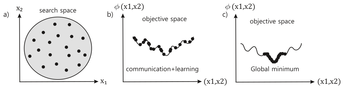
Figure 1 Schematic illustration of (a) randomly distributed particles in model (search) space within a feasible parameter domain (shown as a 2D projection, x1–x2), (b) projection of the particles onto the objective space and (c) convergence of the particles to the global minimum (c), modified from Büyük (2021).

To overcome drawbacks of traditional methods of inversion, PSO has seen a tremendous upsurge in the last decade to invert geophysical data, such as DC-resistivity data (e.g., Fernández Martínez et al., 2010; Peksen et al., 2014; Shaw and Srivastava, 2007), self-potential data (e.g., Fern and Garc, 2010; Monteiro Santos, 2010; Peksen et al., 2011), gravity data (e.g., Essa et al., 2021; Pallero et al., 2015), time-domain electromagnetic data (e.g., Amato et al., 2021; Pace et al., 2022), magnetotelluric data (Grandis and Maulana, 2017; Pace et al., 2019b; Godio and Santilano, 2018) and magnetic data (e.g., Essa and Elhussein, 2018; Liu et al., 2018) and seismological data (e.g., Song et al., 2012). A detailed review on this topic can be found in Pace et al. (2021).

2.2 Pareto-optimal multi-objective particle swarm optimization

Multi-objective optimization, where more than one objective function is optimized, leads to trade-off solutions between competing objectives and not to a single best solution as in single-objective PSO. Multi-objective optimization is defined to obtain the model vector $\mathit{x}=[x_{\mathrm{1}},x_{\mathrm{2}},x_{\mathrm{3}},\mathrm{\dots }{x}_m]$ in a m-dimensional model space, while the objectives in the N-dimensional objective space $\mathit{\varphi }\left(\mathit{x}\right)=\left[{\mathit{\varphi }}_{\mathrm{1}}\right(\mathit{x}),{\mathit{\varphi }}_{\mathrm{2}}(\mathit{x}),{\mathit{\varphi }}_{\mathrm{3}}(\mathit{x}\left)\mathrm{\dots }{\mathit{\varphi }}_N\right(\mathit{x}\left)\right]$ are optimized, simultaneously. The Pareto optimality approach is one of the most successful methods for finding a set of optimal solutions in the feasible search space, as shown schematically in Fig. 2. According to Pareto optimality approach, we say that x_a dominates x_b if and only if ϕ_k(x_a)≤ϕ_k(x_b), k=1, …, N, where N is the dimension of the objective function. We say that x_a is non-dominated and ϕ(x_a) is a non-dominated solution set if there does not exist the condition that ϕ(x_c)<ϕ(x_a), where x_c denotes all possible model vectors. We also say that x_a is Pareto-optimal (Fig. 2a), and ϕ(x_a) is Pareto front or Pareto-optimal set illustrated in Fig. 2b. This indicates the trade-off solutions that conflict with each other in the objective function space, when x_a∈F (feasible region as illustrated in Fig. 2a) is non-dominated. The solution closest to the origin (0, 0) can be considered as the Pareto-optimum solution, within the Pareto-optimal set (Baumgartner et al., 2004; Büyük, 2021, 2024; Reyes-Sierra and Coello Coello, 2006; Schnaidt et al., 2018). Although Pareto optimality is widely used for multi-objective optimization in engineering problems, only a few researchers such as Büyük et al. (2020), Pace et al. (2019a), Schnaidt et al. (2018), Akca et al. (2014), Tronicke et al. (2011), Dal Moro (2010), Kozlovskaya et al. (2007), Paasche and Tronicke (2007) and Moorkamp et al. (2010) integrated global optimization algorithms with the Pareto optimality approach to jointly invert various geophysical data.

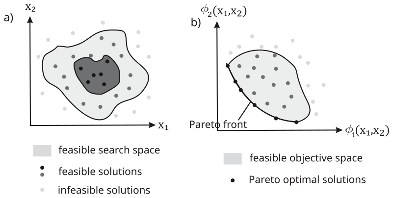
Figure 2 Conceptual illustration of the Pareto-based multi-objective optimization framework. (a) Two-dimensional feasible model (search) space showing feasible and infeasible solutions, modified from Kumar and Minz (2014). (b) Two-dimensional objective space showing the mapped feasible solutions, the Pareto-optimal (non-dominated) solution set, and the Pareto front, modified from Büyük (2021).

3 Description of synthetic data examples

Figure 3a and b presents the synthetic apparent resistivity (ρ_a) and phase (φ) responses, respectively, for 20 periods spanning 10⁻²–10³ s, computed from a synthetic 1D resistivity model ρ(z) (Fig. 3d) that includes low-ρ layers at ∼6–10 km depth. Figure 3c shows the corresponding synthetic RWD curve for 20 frequencies between 5 to 20 s, generated from the 1D shear-wave velocity model V_s(z) (Fig. 3e) designed to mimic the layer-to-layer physical changes implied by the resistivity model. In this example, both models exhibit consistent trends across layers (low-ρ associated with low-V_s, and vice versa) without applying any explicit scaling between parameter types. We refer to this configuration as the coupled case.

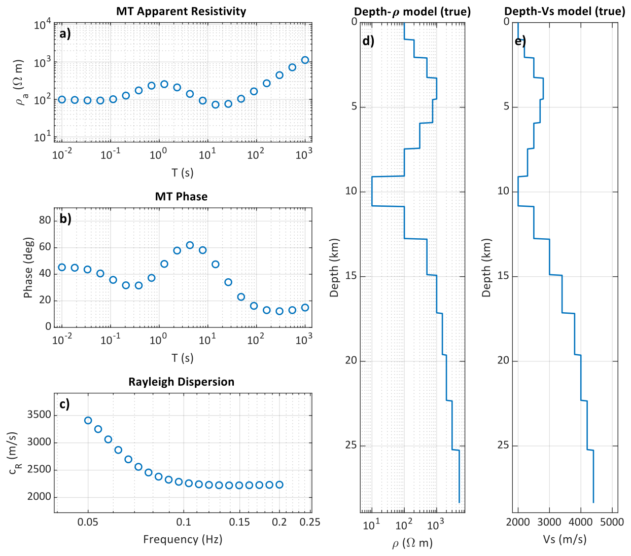
Figure 3 Synthetic (a) apparent resistivities, (b) phase and (c) RWD curve generated from (d) ρ(z) and (e) V_s(z) models, respectively, indicating coupled case.

Figure 4a and b shows the synthetic ρ_a and φ responses for a ρ(z) model containing low-ρ layers (Fig. 4d), while Fig. 4c shows the RWD data generated from a V_s(z) (Fig. 4e) that is intentionally insensitive to those conductive layers. This case is an MT-dominant decoupled scenario, where the model has a pronounced low-ρ zone at ∼6–10 km depth, while V_s(z) remains nearly constant at the same depths (i.e., RWD is weakly sensitive to the resistivity anomaly). We refer to this configuration as decoupled case 1. Conversely, Fig. 5 presents a V_s(z) model with a decrease (Fig. 5e) for which the corresponding ρ(z) (Fig. 5d) does not exhibit a conductive counterpart. This case is an RWD-dominant decoupled scenario, where the model has a pronounced low-V_s zone at ∼6–10 km depth, while ρ(z) remains nearly constant at the same depths (i.e., MT is weakly sensitive to the velocity anomaly). We refer to this configuration as decoupled case 2. Figure 5a and b shows the ρ_a and φ response of the ρ(z); Fig. 5c shows the RWD curve computed from V_s(z) of the decoupled case 2.

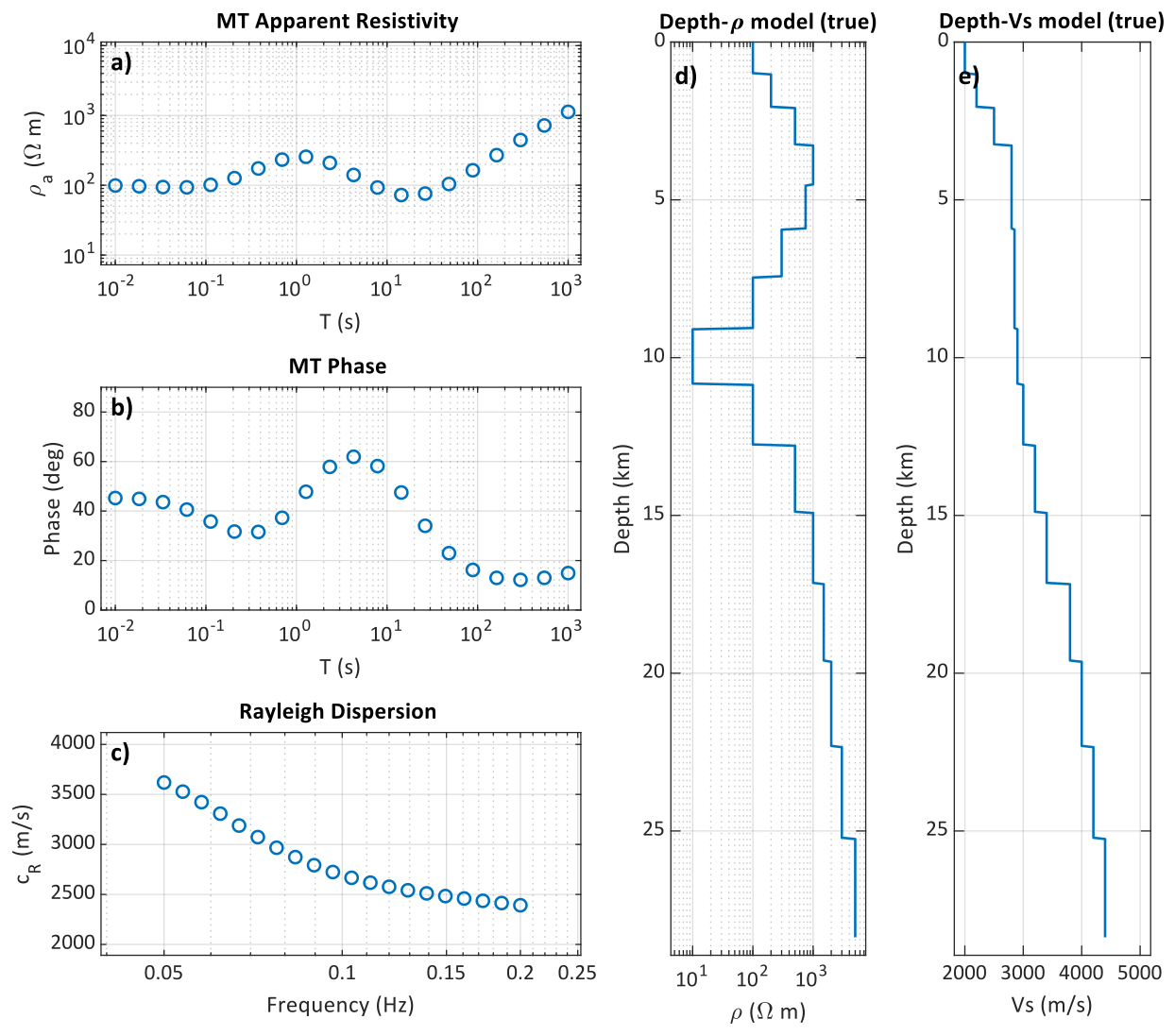
Figure 4 Synthetic (a) apparent resistivities, (b) phase and (c) RWD curve generated from (d) ρ(z) and (e) V_s(z) models, respectively, indicating decoupled case 1.

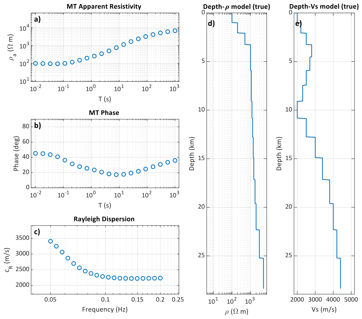
Figure 5 Synthetic (a) apparent resistivities, (b) phase and (c) RWD curve generated from (d) ρ(z) and (e) V_s(z) models, respectively, indicating decoupled case 2.

Synthetic apparent resistivities were computed from 1D magnetotelluric responses using the effective impedance tensor formulation of Berdichevsky et al. (1989), which indicates rotationally invariant impedance derived from the determinant of the impedance tensor. Fundamental-mode dispersion curves were generated using the open-source package SESARRAY developed as part of the SESAME European Project presented by Bard (2000). These forward algorithms provide the synthetic observations used in the Pareto–MOPSO experiments. Although, ρ_a data are sensitive the frequency-dependent, depth-averaged resistivity of the subsurface, similar to how RWD data are sensitive to depth-averaged V_s(z) (Scherbaum et al., 2003; Simpson and Bahr, 2005), we added MT φ to the inversion to constrain the vertical resistivity gradients in case of complex impedance. Therefore, MT input to the inversion includes both ρ_a and φ. These are inverted with the RWD curve (c_R), and the total objective function is composed of three misfit terms corresponding to three datasets of ρ_a, φ and c_R.

4 Description of the field datasets

4.1 Rayleigh wave dispersion curves from earthquake data

In this study, we applied the two-station method, which uses a technique described by McMechan and Yedlin (1981) to obtain the inter-station phase velocities using the codes provided by Herrmann (2002). In this technique, the entire wavefield of the data is transferred to the slowness-frequency domain (p–ω) to pick the RWD curve directly, which involves a linear transformation of the slant stack followed by a 1D Fourier transform. We used broadband data from an earthquake with a magnitude of M_w=6.5 occurred in Italy on 30 October 2016. The earthquake is approximately 1200 km away from the study area, which is located in the south-eastern part of the Biga Peninsula between Ayvacık and Edremit bay in Çanakkale province, Türkiye. The data of this earthquake from these permanent stations are extracted from the waveform database of the Disaster and Emergency Management Presidency (AFAD). Before applying the two-station method, we first removed the mean, trend and instrument response from the earthquake recordings. This method also requires the two stations to be aligned on a path with the epicenter of the earthquake. We found three paths from station BOZC to stations BUHA, STEP and DEMI (hereafter referred to as BOZC_paths), where the azimuthal difference between the source to station-1 and the source to station-2 is less than 2°. We also found for station ECEA to stations STEP and DEMI (hereafter referred to as ECEA_paths) with an azimuthal difference of less than 7°.

4.2 Magnetotelluric data

MT is a passive electromagnetic method that enables to determine the subsurface electrical resistivity ρ(Ωm) by measuring the natural variations of the wide spectrum of electric and magnetic fields induced by natural sources (e.g., solar wind, lightning) (Chave and Jones, 2012; Simpson and Bahr, 2005). Time-varying external electromagnetic fields interact with the conductive Earth and induce secondary currents, whose resulting electric and magnetic fields can be measured at the surface. In the MT method, the Earth can be considered as a transfer function that defines the ratio between orthogonal horizontal electric and magnetic field components (Buttkus, 2000; Cagniard, 1953). The MT method operates over a wide period range, typically from 10⁻⁴ to 10⁴ s, allowing investigation of depths from the near-surface to the upper mantle (Chave and Jones, 2012; Romano et al., 2018). In the MT studies, periods longer than ∼1 s are mainly associated with ionospheric/magnetospheric sources, whereas periods shorter than ∼1 s are predominantly influenced by atmospheric sources such as lightning (Chave and Jones, 2012; Simpson and Bahr, 2005)

We measured MT data at GURE and KULC stations shown in Fig. 4 due to their positions, which are on the BOZC_paths and ECEA_paths, respectively. The MT field data were obtained using a Metronix ADU-07e receiver unit. Sampling rates of 65 536, 16 384, 4096, 1024, 512 and 128 Hz were used to record electromagnetic time series with durations of 2, 4, 8, 16, 32 and 2880 min, corresponding to 48 h at each MT station. The fundamental principle of the MT method is the estimation of the frequency-dependent impedance tensor from simultaneous electric and magnetic fields measurements at the Earth's surface. The Earth modifies the amplitude ratio and phase between these fields (Chave and Jones, 2012; Simpson and Bahr, 2005; Smirnov, 2003). ρ_a and φ are derived from the complex impedance tensor (Z), where the apparent resistivity is frequency-dependent and can be expressed as follows:

$$\begin{array}{}\text{(3)}& {\mathit{\rho }}_{\mathrm{a}}\left(\mathit{\omega }\right)={\displaystyle \frac{\mathrm{1}}{{\mathit{\mu }}_{\mathrm{0}}\mathit{\omega }}}{\left|Z\left(\mathit{\omega }\right)\right|}^{\mathrm{2}}\end{array}$$

and the phase as

$$\begin{array}{}\text{(4)}& \mathit{\phi }\left(\mathit{\omega }\right)={\tan }^{-\mathrm{1}}\left({\displaystyle \frac{\mathrm{Im}\left[Z\right(\mathit{\omega }\left)\right]}{\mathrm{Re}\left[Z\right(\mathit{\omega }\left)\right]}}\right)\end{array}$$

where, ω is the angular frequency, defined as ω=2πf, f is the frequency, and “Re” and “Im” denote the real and imaginary parts of the impedance, respectively. μ₀ is the magnetic permeability assumed to be that of free space ($\mathrm{4}\mathit{\pi }\times {\mathrm{10}}^{-\mathrm{7}}$). Conversion of time series to spectral estimates allows extraction of impedance tensor elements and derivation of ρ_a and φ. MT processing steps were performed using an open-source Python package of SigMT (Ajithabh and Patro, 2023). To estimate the impedance tensor, the time series were segmented into overlapping windows and transformed to the frequency domain using the fast Fourier transform (FFT). Then, power and cross-spectra were computed and stacked to estimate the impedance tensor elements. The effective impedance formulation was used not only for the synthetic examples but also for the field-data inversions, ensuring consistency between the synthetic tests and real-data applications.

5 Site description

The southeastern Biga Peninsula, with its complex structural features of tectonic and magmatic origin, has received considerable attention in several studies (e.g., McKenzie, 1978; Dewey and Şengör, 1979; Taymaz et al., 1991; Okay et al., 1996; Karacık and Yılmaz, 1998; Altunkaynak et al., 2012). As shown in Fig. 6, the simplified map describes the geology of the study site with outcrops of a combination of continental and oceanic crustal units corresponding to metamorphic, magmatic and sedimentary rocks. The magmatic process initiated with the complete closure of the Neo-Tethys Ocean subducted into the Sakarya Zone consisting of the Kazdağ metamorphic complex and formed by the subsequent interaction between crust and mantle (Okay and Satir, 2000; Şengün et al., 2011). After complete closure, a continental collision in N–S compression led to partial melting of the lithospheric mantle (Aldanmaz et al., 2000; Altunkaynak and Genç, 2008; Okay et al., 1996; Yilmaz, 1990). The Kazdağ metamorphic complex has a dome-shaped structure enclosed by a marble-rich sequence (Beccaletto, 2003). The N–S extensional regime occurred after the N–S compressional regime from the early Miocene to the late Pliocene triggered volcanic activities (Aslan et al., 2017; Yilmaz et al., 2001). The phases of volcanism are divided into two: (1) the N–S compressional regime, the result of continental collision, produced andesitic lavas with calc-alkaline characteristics through partial melting (Altunkaynak and Genç, 2008; Yilmaz et al., 2001). The second group of volcanics with potassium-rich basaltic volcanics formed during the extensional regime (Altunkaynak and Genç, 2008; Fytikas et al., 1976; McKenzie and Yılmaz, 1991; Yilmaz, 1990). The sedimentary rocks from the Miocene to the Pliocene were deposited as cover units over the ignimbrites, the last product of volcanism (Seyitoğlu and Scott, 1991). Differently aged continental shallow sediments unconformably cover the metamorphosed units of the Kazdağ metamorphic complex (Altıner et al., 1991).

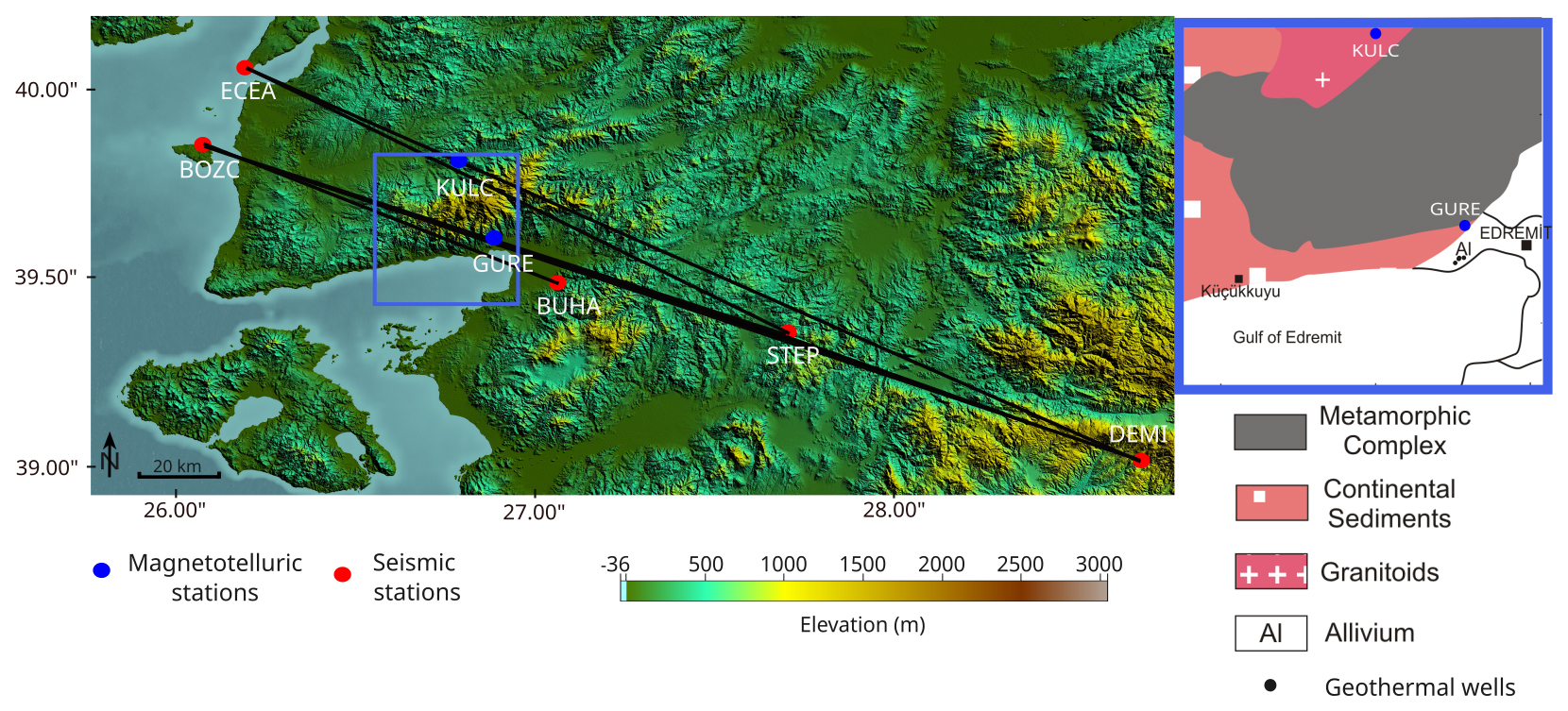
Figure 6 MT and seismic stations over a topographic map obtained from Shuttle Radar Topography Mission (SRTM) data. Black lines indicate the seismic station pairs used to obtain RWD curves. The blue rectangular area shows the geological base map of the southeastern Biga Peninsula reconstructed from Beccaletto (2003) and Yilmaz et al. (2001). The locations of the geothermal wells are from Kaçar et al. (2017).

6 Description of the parameter settings

6.1 Model parameters and misfit functions

The misfit of MT, ϕ_MT(d,m) between the vectors of magnetotelluric data (d) and model response (m), yielding normalized root mean square error (NRMSE) was calculated using:

$$\begin{array}{}\text{(5)}& {\mathit{\varphi }}_{\mathrm{MT}}(\mathit{d},\mathit{m})=\left({\displaystyle \frac{\mathrm{1}}{n}}\sum _{i=\mathrm{1}}^n{\left({\displaystyle \frac{{\mathit{\rho }}_{\mathrm{a},i}^{\mathrm{obs}}-{\mathit{\rho }}_{\mathrm{a},i}^{\mathrm{cal}}}{{\mathrm{\Delta }}_{\mathit{\rho },i}}}\right)}^{\mathrm{2}}+{\displaystyle \frac{\mathrm{1}}{n}}\sum _{i=\mathrm{1}}^n{\left({\displaystyle \frac{{\mathit{\phi }}_i^{\mathrm{obs}}-{\mathit{\phi }}_i^{\mathrm{cal}}}{{\mathrm{\Delta }}_{\mathit{\phi },i}}}\right)}^{\mathrm{2}}\right)\end{array}$$

where n is the number of observations, ${\mathit{\rho }}_{\mathrm{a},i}^{\mathrm{obs}}$ and ${\mathit{\rho }}_{\mathrm{a},i}^{\mathrm{cal}}$ are the observed and calculated apparent resistivities expressed as ${\log }_{\mathrm{10}}({\mathit{\rho }}_{\mathrm{a}}/\mathrm{\Omega }m)$, respectively; ${\mathit{\phi }}_i^{\mathrm{obs}}$ and ${\mathit{\phi }}_i^{\mathrm{cal}}$ are the observed and calculated phases (°), respectively. ${\mathrm{\Delta }}_{{\mathit{\rho }}_{\mathrm{a}},i}$ and Δ_φ,i are the standard deviations of the observed apparent ρ_a and φ, respectively. The misfit of RWD, ϕ_RWD(d,m), was also calculated using as NRMSE as:

$$\begin{array}{}\text{(6)}& {\mathit{\varphi }}_{\mathrm{RWD}}(\mathit{d},\mathit{m})={\displaystyle \frac{\mathrm{1}}{n}}\sum _{i=\mathrm{1}}^n{\left({\displaystyle \frac{c_{{\mathrm{R}}_{p,i}}^{\mathrm{obs}}-c_{{\mathrm{R}}_{p,i}}^{\mathrm{cal}}}{{\mathrm{\Delta }}_{c_{\mathrm{R}},i}}}\right)}^{\mathrm{2}}\end{array}$$

where n is the number of observations, $c_{{\mathrm{R}}_{p,i}}^{\mathrm{obs}}$ and $c_{{\mathrm{R}}_{p,i}}^{\mathrm{cal}}$ are the observed and calculated Rayleigh phase velocities (km s⁻¹), respectively. Δ_c,i is the standard deviations of the observed phase velocities. Equations (5) and (6) were used for both the synthetic tests and the field-data applications to ensure consistency when comparing the modelling results. In practice, Δ values act a scale factor to balance MT and RWD objectives; they can be fixed from measurement uncertainties or estimated via quick perturbation-based calibration around the starting model to stabilize objective magnitudes (Xu, 2009). We used error floors to prevent unrealistically small uncertainties from dominating the misfit. The error floors were set to 5 % for ρ_a, 5° for φ. In regard to the c_R, the robust error-floor strategy proposed by Elston (1992) was employed. This entailed the establishment of a minimum uncertainty level, which was derived from the median absolute deviation (MAD) of the residuals. Apart from the field data, we generated k numbers of random perturbations around the produced synthetic model (x_0,j) as follows: $x_j^{\left(k\right)}=m_{\mathrm{0},j}+\mathrm{pert}({\mathrm{UB}}_j-{\mathrm{LB}}_j){\mathit{ϵ}}_j$, where “UB” and “LB” are the upper and lower boundaries of the model parameters, pert=0.1 and ${\mathit{ϵ}}_j\approx N(\mathrm{0},\mathrm{1})$. This approach is mostly to keep objectives numerically balanced and avoid huge penalties (Pace et al., 2021). Although the estimation of layer thicknesses could lead to a complicated solution (Siripunvaraporn et al., 2005), the layer thicknesses are also estimated by PSO in the modeling stage to couple the ρ and V_s parameters in the corresponding layers. Therefore, coupling is provided by layer thicknesses estimated from the PSO algorithm rather than prescribed spatial locations. Although it was necessary to control the solution sampling with different types of regularization, we used a new method proposed by Büyük (2024) without the need for a subjective and iteration-dependent regularization parameter by adding a smoothness constraint term as a new axis to the objective function space. The smoothness term ϕ_c, was calculated by summing the numerical gradients of the electrical resistivity and seismic velocity parameters as follows:

$$\begin{array}{}\text{(7)}& {\mathit{\varphi }}_c\left(\mathit{m}\right)={\displaystyle \frac{\mathrm{1}}{h}}\sum _{h=\mathrm{1}}^h\left|\mathrm{\Delta }{\log }_{\mathrm{10}}{\mathit{\rho }}_h\right|+{\displaystyle \frac{\mathrm{1}}{h}}\sum _{l=h}^h\left|\mathrm{\Delta }{\log }_{\mathrm{10}}{V}_{s,h}\right|\end{array}$$

with $\mathrm{\Delta }{\log }_{\mathrm{10}}{\mathit{\rho }}_h={\log }_{\mathrm{10}}{\mathit{\rho }}_{h+\mathrm{1}}-{\log }_{\mathrm{10}}{\mathit{\rho }}_h$ and V_s. This equation indicates an additional objective function term that constrains the change in physical parameters to encourage piecewise-smooth layered models. As Eqs. (5) and (6), this equation is the third term of the objective function and forms the third axis in the Pareto space. Therefore, independent minimizations are applied without the need for regularization parameters both in the misfit functions and in the model variation. The optimization is based on the estimation of 47 parameters, including 16 layers of ρ and V_s, as well as a common layer thickness (h) of 15 layers, as generated by the models using synthetic data. The parameter search space of these model parameters that should be restricted to ensure a feasible solution set, was defined in the range log ₁₀[0, 5]Ωm for ρ, and [1.5, 5] km s⁻¹ for V_s to cover realistic values in the crust. The P-wave velocities and densities were calculated using the equations given by Berteussen (1977) as typically observed in the crustal zone.

6.2 MOPSO and Pareto optimality parameters

We used velocity limiting approach proposed by Fan and Shi (2001) to constrain the velocity of particles that tend to explode to large values if the particle is far from the global and local best position. This approach limits the particle velocities as follows: $V_{\max }=+U$ and $V_{\min }=-U$, where $U=(m_{\max }-m_{\min })/N$. m_min and m_max are the lower and upper bounds of the model parameters used to define the search space. For MT modeling, the resistivity bounds were defined as ${\log }_{\mathrm{10}}(\mathit{\rho }/\mathrm{\Omega }m)\in [\mathrm{1},\mathrm{5}]$. For RWD modeling, the shear-wave velocity bounds were defined as $V_{\mathrm{s}}\in [\mathrm{1.5},\mathrm{5}]$ km s⁻¹. N is the interval number, which was set to 10. We used modified velocity equation of the Eq. (1), proposed by Clerc and Kennedy (2002) to obtain solutions without trapping a local minimum due to premature convergence, as defined below:

$$\begin{array}{}\text{(8)}& {\mathbf{V}}_i^{k+\mathrm{1}}=\mathit{\chi }\left[{\mathbf{V}}_i^k+c_{\mathrm{1}}{\mathit{\gamma }}_{\mathrm{1}}\left({\mathit{x}}_{\mathrm{pbest},i}-{\mathit{x}}_i^k\right)+c_{\mathrm{2}}{\mathit{\gamma }}_{\mathrm{2}}\left({\mathit{x}}_{\mathrm{gbest}}-{\mathit{x}}_i^k\right)\right]\end{array}$$

where, χ is the constriction factor expressed as: $\mathit{\chi }=\mathrm{2}/(k-\mathrm{2}+\sqrt{k^{\mathrm{2}}-\mathrm{4}k})$ under the condition that $k=c_{\mathrm{1}}+c_{\mathrm{2}}>\mathrm{4}$. Therefore, we used c₁ and c₂ as 2.05, i.e., k=4.1 and χ=0.7298 following Clerc and Kennedy (2002). The number of particles was set to 100, which is consistent with the general guidance of Piotrowski et al. (2020). They recommend using an initial guess of 70–100 particles when no prior knowledge is available. The particle positions were initialized by randomly sampling within the prescribed parameter bounds for each model parameter. Initial velocities are set to zero and particles that violate bound constraints are repaired by clipping them to the nearest feasible bound. A two-stage schedule was used to accelerate convergence followed by Deb and Padhye (2010). First, an exploration phase with larger velocity limits and a higher mutation probability, second, an exploitation phase with reduced step sizes and mutation was used. In Stage-1(exploration), we used larger velocity bounds: $v_{\max }^{\left(\mathrm{1}\right)}=\mathrm{0.25}(\mathrm{UB}-\mathrm{LB})$. We also utilized higher mutation probability decaying linearly. If we consider that ${\mathrm{it}}_{\mathrm{switch}}=\mathrm{0.4}\times \mathrm{MaxIt}$, where MaxIt is the maximum number of iterations, $p_{\mathrm{mut}}\left(\mathrm{it}\right)=\max \left({\mathrm{pMin}}_{\mathrm{1}}p{\mathrm{0}}_{\mathrm{1}}\right(\mathrm{1}-\mathit{\tau }\left)\right)$, $\mathit{\tau }=\mathrm{it}/{\mathrm{it}}_{\mathrm{switch}}$ with p0₁=0.12, pMin₁=0.04, where “it” is the iteration number. In the Stage-2 (exploitation) a smaller velocity bounds were defined as follows: $v_{\max }^{\left(\mathrm{2}\right)}=\mathrm{0.1}(\mathrm{UB}-\mathrm{LB})$, and lower mutation probability $p_{\mathrm{mut}}\left(\mathrm{it}\right)=\max \left({\mathrm{pMin}}_{\mathrm{2}}p{\mathrm{0}}_{\mathrm{2}}\right(\mathrm{1}-\mathit{\tau }\left)\right)$, $\mathit{\tau }=(\mathrm{it}-{\mathrm{it}}_{\mathrm{switch}})/(\mathrm{MaxIt}-{\mathrm{it}}_{\mathrm{switch}})$ with p0₂=0.06, pMin₁=0.01. Therefore, mutation perturbs a randomly selected model parameters m_j with probability p_mut via $m_j=m_j+\mathrm{0.05}({\mathrm{UB}}_j-{\mathrm{LB}}_j)$. Iteration was terminated at 150 iterations for both synthetic and field datasets as one way of limiting the maximum number of iterations (Reyes-Sierra and Coello Coello, 2006) and 10 experimental solutions were generated repeatedly. In all tests, we used a fixed iteration budget rather than an adaptive termination criterion. Therefore, convergence was not used as a stopping rule.

After each iteration, objective function space is divided into hyper-rectangles, to each of which control solutions are added (Coello Coello et al., 2004; Coxeter, 1973). One-tenth of the number of particles was defined as the number of hyper-rectangles for each objective function. The roulette wheel selection, one of the scheme theorems proposed by Coello Coello et al. (2004), which is based on the rational division of the segments of the wheel according to the number of non-dominated solutions in each of the hyper-rectangles, was used to select a leader for MOPSO. According to this theorem, the ratio decides the selection probability (Ps) of an individual hyper-rectangle as follows: $\mathrm{Ps}\left(k\right)=n_k/\sum _{i=\mathrm{1}}^N{n}_i$; i=1, 2, …, N, where, N is the number of hyper-rectangles with non-dominated solutions n_k is the number of non-dominated solutions of the kth hyper-rectangle (Rao, 2009). A leader is randomly determined from the selected hyper-rectangle. In the dominance test, we used the raw misfits of the objectives, however, normalized misfits were used in the grid assignment to improve the crowding grid when objectives have different numerical scales. To improve clarity and reproducibility, we provide the pseudocode for the proposed Pareto–MOPSO joint inversion workflow in Fig. S1 in the Supplement.

The final representative solutions include a “utopia” model that minimizes the sum of two datasets $\sqrt{{\mathit{\varphi }}_{\mathrm{MT}}^{\mathrm{2}}+{\mathit{\varphi }}_{\mathrm{RWD}}^{\mathrm{2}}}$, and a “compromise(knee/score)” model that minimizes the sum of per-iteration normalized objectives, including smoothness term as follows: $\sum _k{\mathit{\varphi }}_k-{\mathit{\varphi }}_{\min ,k}/{\mathit{\varphi }}_{\max ,k}-{\mathit{\varphi }}_{\min ,k}$. We summarize uncertainty by treating the Pareto repository as an ensemble of non-dominated solutions. After mapping all archived models onto a common depth grid, we compute the depth-wise percentiles of ρ(z) and V_s(z). We then report the P₁₀–P₉₀ envelope, which contains the central ∼80 % of Pareto-optimal profiles (Fathy et al., 2024; Gao et al., 2023). The P₁₀–P₉₀ Pareto envelope offers quantitative insights into depth-dependent parameter uncertainty by delineating a plausible range of admissible models. Narrow envelopes indicate depths where the parameters are consistently recovered (higher resolution/stronger constraint), whereas wide envelopes indicate depths where non-uniqueness is significant and multiple alternative structures remain compatible with the data and the multi-objective trade-offs. The Pareto-median is plotted as a robust representative profile alongside the envelope (Brazauskas and Serfling, 2000). The Pareto-median band effectively captures the predominant depth-wise trend of the physical parameters and reliably represents the overall structural evolution with depth. To quantitatively evaluate the joint inversion outcomes, we employed the Generational Distance (GD) metric introduced by Van Veldhuizen (1999) as a convergence indicator for the obtained Pareto-optimal solution sets. The goal of the GD method is to evaluate the proximity of an estimated Pareto front to a reference front. The GD method accomplishes this by first calculating the Euclidean distance to the nearest point on the reference Pareto front. Then, the distances are aggregated to provide a comprehensive measurement of the front's deviation from the reference (Büyük, 2024; Coello et al., 2004). Lower GD values reflect superior solution performance, while higher values illustrate the extent to which the solution deviates from the Pareto front (Coello et al., 2004; Van Veldhuizen, 1999).

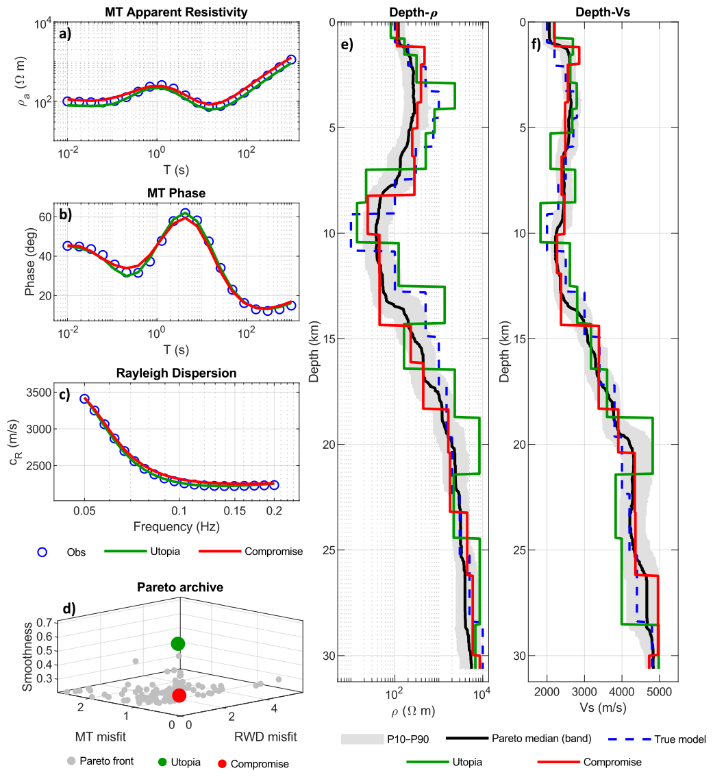
Figure 7 Results for noise-free coupled case. (a) Apparent resistivity and (b) phase data and (c) RWD fit with the predicted responses of the selected representative solutions. (d) Three-objective Pareto archive, highlighting the utopia and compromise solutions. (e) ρ(z) and (f) V_s(z) models for the true model and the selected utopia and compromise solutions, together with the P₁₀–P₉₀ envelope and the Pareto-median profile from the repository.

7 Results and discussions

7.1 Coupled case

7.1.1 Noise-free analysis

Figure 7a–c shows the noise-free outputs of the coupled case, which agree very well with the synthetically generated observations. As illustrated in Fig. 7d, the Pareto archive is indicative of the objective space, which involves the minimization of the objective function terms of the utopia and compromise within the Pareto-optimal set. Figure 7e and f shows the ρ(z) and V_s(z) models of the true, utopia, and compromise model with P₁₀–P₉₀ envelope and Pareto-median. As anticipated for a problem with such extensive parameterization (47D), the findings suggest that the algorithm attained an optimal data fit, while simultaneously identifying a non-unique set of permissible models. The apparent resistivity is matched particularly well at intermediate to long periods (Fig. 7a). This finding suggests that the inversion effectively recovers the bulk resistivity contrasts that govern the deeper MT response. The phase is also well reproduced, including the main peak and the long-period decrease. Minor deviations from this pattern are observed in the transition region, where the phase exhibits a high degree of sensitivity to the precise positioning of resistivity contrasts and layer boundaries (see Fig. 7b). The RWD curve demonstrates a high degree of compatibility, with predicted phase velocities that closely align with the observed curve (see Fig. 7c). This indicates that the recovered V_s(z) structure within the depth sensitivity range of the dispersion is stable and strongly constrained. Since the fundamental mode primarily detects broad depth averages rather than sharp discontinuities, slight variations in layer boundaries and magnitude of steps can remain dispersion-equivalent. This is reflected by the range of acceptable V_s(z) profiles. The Pareto archive (Fig. 7d) shows the expected trade-off surface between MT misfit, RWD misfit, and smoothness. The utopia solution corresponds to the archive member that is closest to the MT–RWD origin, representing the optimal balance between the two data misfits. Meanwhile, the compromise solution reflects a more balanced trade-off when smoothness is also taken into consideration. The fundamental premise is that both are derived from the Pareto optimal solution set, implying that enhancing one objective invariably leads to a corresponding degradation in at least one other objective.

Depth-dependent models (Fig. 7e and f) indicate that the major trends of the true ρ(z) and V_s(z) structures are recovered, while some layer values and boundary depths differ between representative solutions. This is an expected outcome resulting from the interplay of trade-offs among ρ and V_s when thicknesses (h) are inverted jointly. To quantify this non-uniqueness, Pareto archive is summarized by mapping all repository models onto a common depth grid. The P₁₀–P₉₀ envelope is then computed, along with Pareto-median profile. The P₁₀–P₉₀ band demonstrates a tendency to widen during certain transitions, suggesting that while the data are highly fitted, the underlying structure, particularly the precise magnitude and position of step changes, remains less uniquely determined. This phenomenon is not only permissible but also serves as a notable strength of the presented method, as it circumvents the tendency toward over-interpretation of a singular “best” layered model as indicated by Schnaidt et al. (2018). The Pareto-median profile has been shown to closely track the true ρ(z) and V_s(z) structures over most depths. This finding suggests that the Pareto-optimal solution set ensemble produced by the Pareto–MOPSO search is capable of not only fitting the data, but also centering around the generating model in parameter space. It is imperative to acknowledge that this behavior is anticipated for idealized tests of the noise-free case, with this behavior mainly reflecting the consistency of the forward responses with the designated parameterization and bounds. In the context of field data, the Pareto-median should be interpreted as a robust representative of the non-dominated ensemble, as opposed to being regarded as a unique estimate of the true Earth model.

7.1.2 Noise-sensitivity analysis

A noise-sensitivity analysis was performed by the perturbing of both MT and RWD observations with equal-amplitude, normalized Gaussian noise (0 %–40 %). The 20 % noise scenario is presented as a representative intermediate-noise example (see Fig. 8), as it marks the transition where uncertainty bands broaden and Pareto trade-offs become more pronounced while still maintaining meaningful data constraints. The remaining noise cases (5 %, 10 %, and 40 %) are reported in Figs. S2–S4. A comparison of the compromise solution and the noise-added outputs of the utopia solution reveals a strong agreement with the synthetically generated observations. The apparent resistivity curves demonstrate a high degree of alignment across the entire period range, encompassing both the mid-period minimum and the long-period upturn. The phase responses demonstrate a comparable degree of agreement, exhibiting the characteristic phase peak near intermediate periods and the subsequent decay toward long periods with a high degree of precision. Minor deviations from this pattern are observed around the phase maximum and shoulder regions, which are traditionally the most sensitive components of the MT response to ρ–h trade-offs (Degroot-Hedlin and Constable, 1990; Kang et al., 2017). However, the predicted curves align with the data trend within the limits. The RWD curves are also fitted closely, capturing the strong decrease of phase velocity from low to mid frequencies and the flattening at higher frequencies. It is evident that minor residual mismatches in the curvature of the dispersion curve are consistent with non-uniqueness in layered dispersion inversion. In this scenario, it is observed that multiple V_s–h combinations can yield very similar fundamental-mode responses as noted by Foti et al. (2009) and Roy et al. (2013).

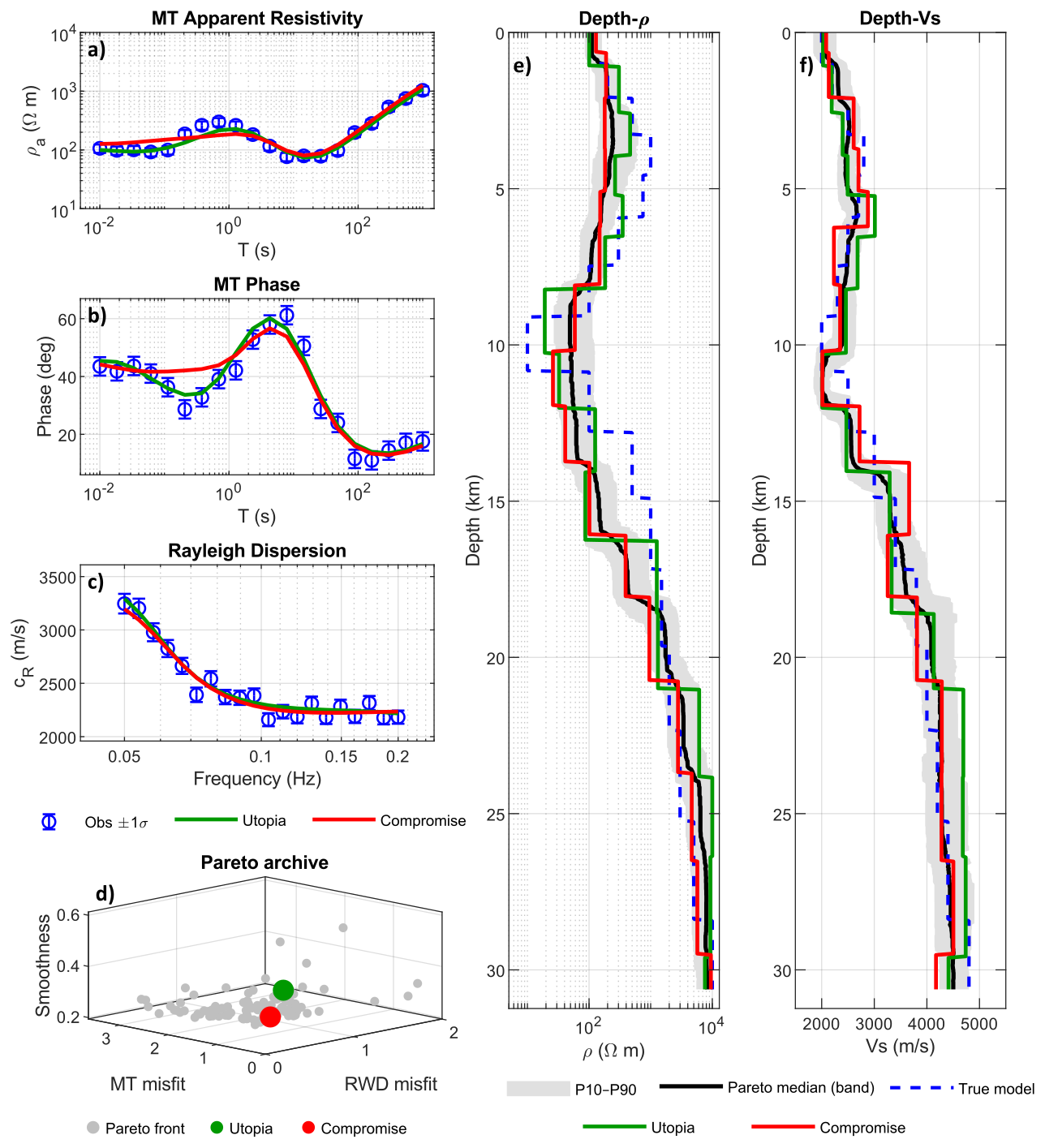
Figure 8 Results of noise-sensitivity example for the 20 % noisy-coupled case (representative intermediate-noise level). (a) Apparent resistivity and (b) phase data and (c) RWD fit with the predicted responses of the selected representative solutions. (d) Three-objective Pareto archive, highlighting the utopia and compromise solutions. (e) ρ(z) and (f) V_s(z) models for the true model and the selected utopia and compromise solutions, together with the P₁₀–P₉₀ envelope and the Pareto-median profile from the repository.

The ρ(z) and V_s(z) panels demonstrate that the representative models fall or outside within the ensemble uncertainty indicated by the P₁₀–P₉₀ envelope. At low noise levels, the utopia and compromise models remain largely confined within the P₁₀–P₉₀ envelope. This indicates that these solutions are not only optimal in the objective space, but also representative of the central tendency of the Pareto ensemble in model space. Conversely, as the noise level increases, both solutions demonstrate more frequent and more pronounced departures from the P₁₀–P₉₀ band, particularly in the ρ(z) and around layer-transition depths. This pattern indicates that the inversion becomes increasingly governed by noise-induced trade-offs, such that mathematically admissible solutions are less consistently supported by the ensemble as a whole. Concurrently, the Pareto archives undergo a transition from a relatively compact and organized distribution under low-noise conditions to a broader and more scattered cloud at higher noise levels as reported by Witting et al. (2012). This shift is indicative of a substantial increase in non-uniqueness and weakening data control on the recovered structures. Taken together, these results suggest that the geometry of the Pareto archive and the position of the utopia/compromise solutions relative to the P₁₀–P₉₀ envelope provide a useful diagnostic measure of inversion stability. In this context, solutions remaining within the ensemble envelope can be regarded as more robust and representative; whereas those falling outside this should be interpreted with caution as noise-sensitive and structurally less constrained.

Figure 9 provides a summary of the impact of increasing observational noise on the joint Pareto–MOPSO inversion in terms of (a) utopia-point objective values, (b) Pareto-front drift, and (c) ensemble model uncertainty. As the noise level increases from 0 % to 40 %, the utopia misfits for both MT and RWD rise systematically (see Fig. 9a). It is noteworthy that the RWD misfit exhibits a faster rate of inflation compared to the MT misfit at moderate-to-high noise levels. This observation indicates a greater sensitivity of the RWD objective to noise in the given configuration. The corresponding Pareto-front deviation, quantified by the Generational Distance (GD) relative to the noise-free reference Pareto-front, increases markedly up to ∼20 % noise and then approaches a plateau towards 40 % (Fig. 9b). This phenomenon indicates a shift from a data-dominated regime (low noise) to a noise-limited regime (≥20 %), where additional increases in noise do not result in a significant shift of the Pareto front in normalized objective space. This robustness is a key advantage of the Pareto–MOPSO, as it allows the inversion to maintain a diverse set of viable solutions rather than collapsing to a single, potentially biased estimate, even when noise levels exceed 20 %. The mean P₁₀–P₉₀ bandwidth across depth, which is indicative of model uncertainty, reveals a pronounced contrast between ρ and V_s parameters (Fig. 9c). The ρ ensemble demonstrates significantly greater uncertainty (in log ₁₀ decades) and displays a modest increase in response to noise, which is consistent with amplified ρ–h trade-offs under noisy MT responses. In contrast, the V_s bandwidth remains comparatively small and nearly invariant across noise levels. This finding indicates that the RWD data provide relatively robust constraints on depth-averaged shear velocities relatively robustly within the tested parametrization and regularization. Nevertheless, it is important to note that RWD inversion is inherently non-unique due to the fact that numerous layered V_s–h models have the capacity to reproduce analogous fundamental-mode curves. This ambiguity is further exacerbated in the presence of noisy observations (Dal Moro, 2010; Kozlovskaya et al., 2007). The findings of this study indicate a distinct divergence between data-space sensitivity and model-space uncertainty. Despite the RWD objective demonstrating a more rapid deterioration with increasing noise, indicating stronger noise sensitivity in the RWD misfit, the MT-derived ρ(z) models exhibit a larger increase in ensemble uncertainty. The shared layer-thickness parameterization suggests that noise perturbs the RWD fit more directly, whereas in the MT branch it more strongly enhances the ρ–h trade-off, leading to broader uncertainty in the recovered ρ(z) structure.

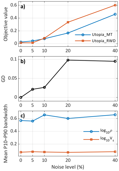
Figure 9 Noise-sensitivity analysis for the Pareto–MOPSO joint inversion, (a) objectives of the utopia solution, (b) Generational Distance (GD) of the Pareto front, (c) model uncertainty from mean P₁₀–P₉₀ bandwidth as a function of noise level.

7.1.3 Layering-sensitivity analysis

In order to maintain identical noise-free synthetic observations and allow layer thicknesses to be optimized, a joint inversion of the datasets with varying parameterizations (h=8, 12, 18, 22) was conducted. For the purpose of clarity, the results obtained with the reference parameterization (h=18 layers) are shown in Fig. 10. This parametrization is indicative of an intermediate-complexity model. The results for alternative layer numbers are provided in Figs. S5–S7 to demonstrate the sensitivity of the recovered models and Pareto trade-offs to the chosen parameterization.

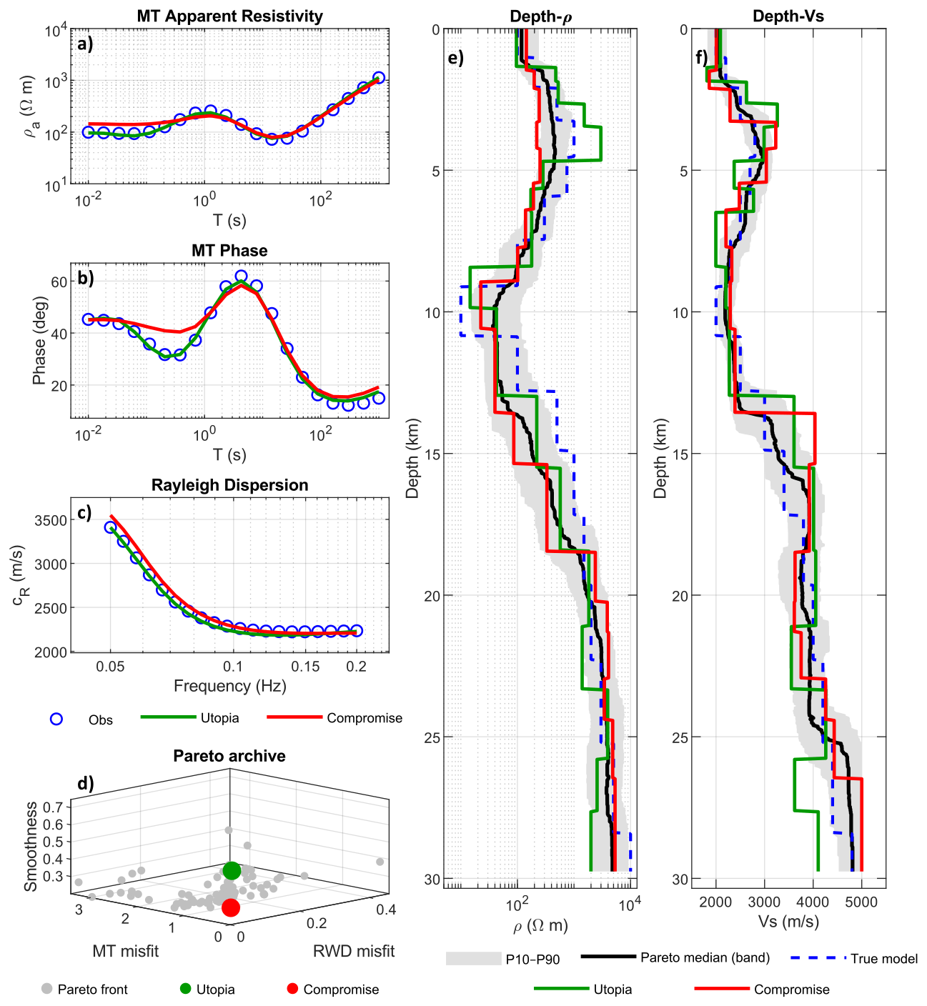
Figure 10 Results of layering-sensitivity example for the h=18 layers (representative an intermediate-complexity model). (a) Apparent resistivity and (b) phase data and (c) RWD fit with the predicted responses of the selected representative solutions. (d) Three-objective Pareto archive, highlighting the utopia and compromise solutions. (e) ρ(z) and (f) V_s(z) models for the true model and the selected utopia and compromise solutions, together with the P₁₀–P₉₀ envelope and the Pareto-median profile from the repository.

The findings reveal that the data-space fits for MT and the RWD curves are comparable, suggesting that the observations primarily constrain the gross-scale ρ(z) and V_s(z) structure. This indicates that the detailed layering is not uniquely determined by these observations. The primary effect of modifying the number of layers is manifested in the model domain and in the distribution of the Pareto archive. When h=8, the parameterization is relatively coarse, resulting in smoother models but also a more biased representation of sharp contrasts. A number of depth intervals exhibit systematic deviations from the true profile, as a limited number of layers are incapable of reproducing the true stepwise structure. Furthermore, the persistence of data fidelity issues is particularly problematic in the context of compromise solutions. It is evident that increasing layer number (h=12) significantly enhances the capacity to depict intermediate-depth transitions with a reduced number of systematic offsets, while preserving a relatively compact ensemble (narrower P₁₀–P₉₀ in key intervals). This suggests a more optimal equilibrium between flexibility and stability. For higher parameterizations (h=18 and especially h=22), the inversion acquires supplementary degrees of freedom although the visual enhancement of the fits is evident. The phenomenon under consideration manifests as more pronounced layer-to-layer oscillations and an increasingly intricate ensemble. The P₁₀–P₉₀ envelope tends to broaden, although the utopia–compromise convergence becomes more pronounced. This reflects stronger trade-offs between fit and smoothness and an expansion of the non-unique solution space. In essence, the presence of additional layers, beyond an intermediate layer count, primarily leads to an increase in model ambiguity rather than enhancing the extraction of information from the same data. The findings of this study suggest that an intermediate parameterization (h≈12–18 layers) provides the most robust compromise. This parameterization is flexible enough to capture the main depth variations indicated by MT and RWD data, but constrained enough to avoid excessive variability in the recovered models.

Figure 11 quantifies the sensitivity of the joint Pareto–MOPSO inversion to the selected number of inversion layers using three complementary metrics: (a) the utopia-point objective values for MT and RWD, (b) the GD values of the resulting Pareto front relative to the reference (h=15) front, and (c) the mean P₁₀–P₉₀ uncertainty bandwidth of the recovered models. As demonstrated in Fig. 11a, the utopia MT objective demonstrates a tendency to augment with increasing parameterization, a finding that aligns with the augmented degrees of freedom facilitating more precise alignments with the MT responses. In contrast, the RWD utopia objective is not strictly minimized at the true layer count (h=15). This phenomenon can be attributed to the fact that the utopia solution is selected from a multi-objective trade-off (MT, RWD, and smoothness) rather than by minimizing the RWD misfit alone. Consequently, the “closest-to-utopia” solution at h=15 can emphasize improved MT fit and/or smoother models while accepting a slightly higher RWD misfit. This indicates that additional degrees of freedom do not simply reduce both misfits simultaneously; instead, they modify the trade-off balance between the two datasets. As illustrated in Fig. 11b, the overall Pareto-front set exhibits the highest degree of consistency with the reference at h=15 (GD≈0 by construction). Conversely, under-parameterization (e.g., h=8–12) and over-parameterization (e.g., h=18–22) result in increasingly larger deviations of the Pareto front. The GD results suggest that the Pareto front does not converge monotonically toward a superior solution as the number of layers increases. Instead, an intermediate parameterization yields the closest and most stable front relative to the reference, whereas both under-parameterized and over-parameterized cases deviate more strongly. As illustrated in Fig. 11c, model uncertainty is found to be strongly parameter-dependent for ρ but comparatively stable for V_s. The P₁₀–P₉₀ envelopes reveal that the dominant effect of layer-number variation is expressed in the ρ(z) model space rather than in the V_s(z) model space. While the V_s uncertainty remains narrow and nearly invariant, the log ₁₀ρ bandwidth is consistently larger. This confirms that the MT branch remains more vulnerable to parameter trade-offs under the shared thickness parameterization.

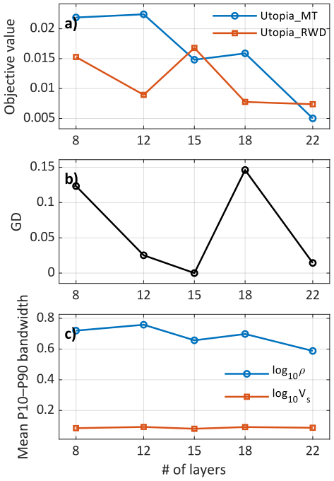
Figure 11 Layering-sensitivity analysis for the Pareto–MOPSO joint inversion, (a) objectives of the utopia solution, (b) Generational Distance (GD) of the Pareto front, (c) model uncertainty from mean P₁₀–P₉₀ bandwidth as a function of layer numbers.

The layer-number experiments indicate that increasing parameterization enhances data-space flexibility. However, this does not result in a monotonic improvement in joint inversion quality. While higher layer counts generally permit lower objective values, they also increase model-space ambiguity, particularly for ρ(z) models. This phenomenon is evidenced by the broader P₁₀–P₉₀ envelopes for log ₁₀ρ in comparison to V_s, suggesting that the MT branch is more profoundly influenced by ρ–h trade-offs within the framework of shared layer-thickness. The Pareto archives further suggest that intermediate parameterizations produce a more compact and stable trade-off structure, whereas excessively coarse models are too restrictive and excessively fine models introduce additional non-uniqueness. The GD metric consistently indicates that the closest and most stable Pareto front is obtained at an intermediate layer number rather than at the maximum complexity tested. The findings of these tests suggest that the optimal parameterization is selected by balancing the reduction of misfit with the stability of the ensemble and the representativeness of the model space. Consequently, within the framework of field-data joint inversions, it is imperative to conduct a robustness test by repeating the joint MT–RWD inversion with multiple alternative layer counts. This is primarily because, in the absence of such a test, the recovered models and uncertainty structure may be indicative of parameterization choices rather than data-driven information content.

7.2 Decoupled cases

7.2.1 Case 1

In the coupled case, systematic noise- and layer-number sensitivity analyses were performed to characterize the stability of the proposed joint Pareto–MOPSO scheme. In the context of the decoupled case, our objective is not to exhaustively re-map robustness, but rather to illustrate how the trade-off structure undergoes modification when the two datasets favor divergent structural scales. Consequently, a representative mini-test is presented at noise-free, 10 %, and 20 % noisy data, which is sufficient to illustrate the characteristic Pareto drift, the redistribution of misfit between MT and RWD, and the associated uncertainty envelope. Furthermore, when considering both the noise-sensitivity experiments and the layering-parameterization tests, it becomes apparent that the utopia solutions provide superior fits and demonstrate the closest convergence toward the true model with Pareto-median within the P₁₀–P₉₀ envelope consistently. Consequently, we adopt the utopia solutions, with Pareto-median and uncertainty via the Pareto ensemble (P₁₀–P₉₀ envelopes), as the preferred model and illustration for the subsequent inversion of the decoupled cases and field data.

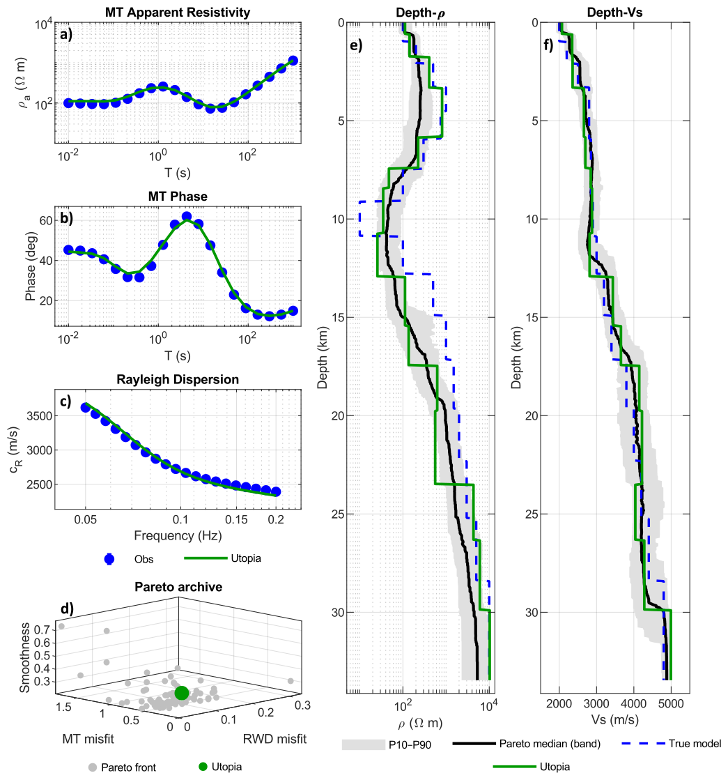
Figure 12 Results of the noise-free decoupled case 1. (a) Apparent resistivity and (b) phase data and (c) RWD fit with the predicted responses of the utopia solution. (d) Three-objective Pareto archive, highlighting the utopia solution. (e) ρ(z) and (f) V_s(z) models for the true model and the selected utopia solution, together with the P₁₀–P₉₀ envelope and the Pareto-median profile from the repository.

Figure 12 summarizes the results for the decoupled case 1 under the noise-free datasets. The results of the remaining tests, incorporating both 10 % and 20 % noisy data, are presented in Figs. S8 and S9. In all cases, the selected utopia solution reproduces the MT and RWD curve trend reasonably well, indicating that a Pareto-optimal solution can achieve low misfits for both datasets simultaneously. The synthetic tests of decouple case 1 demonstrate that the joint Pareto–MOPSO inversion does not artificially enforce a common anomaly in both physical parameters when the underlying structure is genuinely decoupled. In the noise-free case, the conductive anomaly is predominantly recovered in the ρ(z), while no equivalent low-V_s feature is introduced in the V_s(z) structure. This finding suggests that the inversion preserves parameter-specific sensitivity rather than imposing a false cross-property correspondence. With increasing noise (10 %-20 %), the ρ(z) becomes progressively more diffuse and uncertain, as reflected by the widening P₁₀–P₉₀ envelope, whereas the V_s(z) remains comparatively stable apart from minor noise-induced fluctuations, as observed in coupled case. The Pareto archive becomes more scattered simultaneously, indicating increased non-uniqueness. However, the solutions do not collapse into an artificially coupled low-ρ/low-V_s interpretation. The findings indicate that the proposed framework is capable of differentiating between decoupled electrical and mechanical structures. However, a marked decline in the robustness of the model parameters of the MT branch is observed as the level of noise increases.

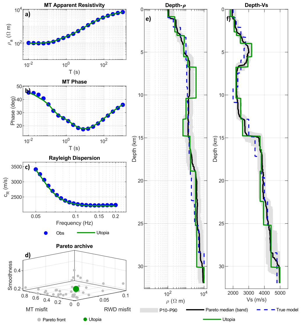
Figure 13 Results of the noise-free decoupled case 2. (a) Apparent resistivity and (b) phase data and (c) RWD fit with the predicted responses of the utopia solution. (d) Three-objective Pareto archive, highlighting the utopia solution. (e) ρ(z) and (f) V_s(z) models for the true model and the selected utopia solution, together with the P₁₀–P₉₀ envelope and the Pareto-median profile from the repository.

7.2.2 Case 2

Figure 13 provides a synopsis of the outcomes derived from the decoupled case 2 under the noise-free datasets. The results of the remaining tests (10 % and 20 %) are displayed in Figs. S10 and S11. In all three cases, the selected utopia solution reproduces the MT curves and the RWD trend reasonably well, thereby confirming that the Pareto search can still identify a low-misfit compromise in the data space even when the underlying structural sensitivities of MT and RWD are mutually inconsistent. The apparent resistivity curves are reproduced with generally good agreement, indicating that the joint inversion preserves the overall MT response even though the synthetic anomaly is not primarily expressed in ρ(z) model. The phase data are also fitted satisfactorily, suggesting that the MT branch remains stable and does not introduce a spurious conductive structure in response to the low-V_s anomaly. The RWD curves effectively capture the predominant trend of the synthetic observations, thereby confirming that the low-V_s anomaly is predominantly resolved by the RWD data. However, it is important to note that the quality of the fit gradually deteriorates as the level of noise increases. The Pareto archive undergoes an evolution from a compact and well-organized trade-off surface in the noise-free case to a broader and more scattered distribution under 10 %–20 % noise. This shift reflects increasing non-uniqueness and weaker data control. The recovered ρ(z) model maintains a close approximation to the true structure and does not exhibit a significant artificial conductive anomaly, suggesting that the inversion does not force a false low-ρ counterpart to the V_s anomaly. The low-V_s predominantly recovered in the V_s(z) model. However, as the noise level increases, the boundaries of the low-V_s become more diffuse, and the uncertainty envelope expands.

The second decoupled tests demonstrate that the inversion framework is capable of recovering a low-V_s anomaly without introducing a spurious conductive counterpart in the ρ(z) model. In the absence of noise, the V_s anomaly is accurately recovered, while the ρ(z) structure maintains proximity to the true, non-anomalous resistivity profile. As the noise level increases (10 %–20 %), the Pareto archive becomes increasingly dispersed, and the V_s uncertainty broadens, particularly at the anomaly depths. However, the solutions maintain the inherently decoupled nature of the synthetic model. This finding suggests that the method respects parameter-specific sensitivity and does not force an artificial low-ρ/low-V_s correspondence when such coupling is absent in the true structure.

7.3 Benchmark comparison and computational performance

Following a thorough evaluation of the Pareto–MOPSO joint inversion under both coupled and decoupled synthetic scenarios, a comparative analysis was conducted with the performance of a deterministic Gauss–Newton (GN) inversion. The GN inversion was implemented with the same forward operators and parameterization. Since GN requires a scalar objective, we employed a normalized weighted-sum formulation that combined the same weights for the misfits in the MT and RWD data to prevent one dataset from dominating the others arbitrarily. The inversion was initialized from a homogeneous reference model, with all resistivity layers set to 100 Ωm, all V_s layers set to 3000 m s⁻¹, and all layer-thickness parameters set to 2000 m. The same model was also used as the reference model for regularization. To stabilize the inversion, first-difference smoothness regularization was applied to the log ₁₀ρ and log ₁₀V_s models, together with a weaker smoothness constraint on layer thickness. The corresponding regularization coefficients were set to λ=0.25 and λ_h=0.1. A Levenberg-type damping scheme was used within the Gauss–Newton iterations, with an initial damping factor of 10⁻² and allowable bounds between 10⁻⁶ and 10². The inversion was run for 150 iterations, consistent with the Pareto–MOPSO implementation. The Jacobian matrix was calculated by finite differences, and parallel forward evaluations were employed to reduce the computational cost.

Figure 14 shows the results of benchmarking the joint inversion of the MT and RWD data using the GN scheme. Overall, the GN solution demonstrates a high degree of compatibility with the observations, exhibiting an optimal alignment across the entire period and frequency ranges (see Fig. 14a–c). However, Fig. 14 highlights several limitations of the equal-weighted Gauss–Newton (GN) joint inversion when compared with the Pareto–MOPSO framework. The ρ(z) structure is reproduced reasonably well (see Fig. 14e), whereas the V_s(z) model converges to a smoother and partly shifted solution that departs from the true layered structure (see Fig. 14f). In particular, it fails to reproduce the shallow high-V_s and underestimates the intermediate-depth low-V_s anomaly, yielding an overly smoothed V_s profile. By contrast, the Pareto–MOPSO solutions preserve the main velocity contrasts more clearly while maintaining a similarly strong data fit. This comparison shows that, while GN is effective at reducing total data misfit, it is still more likely to converge on a V_s model that is locally acceptable but less representative of the structure as a whole. This discrepancy is likely indicative of the inherently non-unique nature of RWD inversion, wherein multiple layered V_s–h combinations can generate RWD curves with a high degree of similarity. Such non-uniqueness and inter-parameter trade-offs in joint MT–RWD inversion are well documented (e.g., Moorkamp et al., 2010) and should therefore be regarded as intrinsic to the inverse problem rather than as a limitation of the forward solver. A number of strategies can be proposed to facilitate the implementation of this process. These include the tuning of the regularization applied to layer thickness or the constraining of the admissible thickness range.

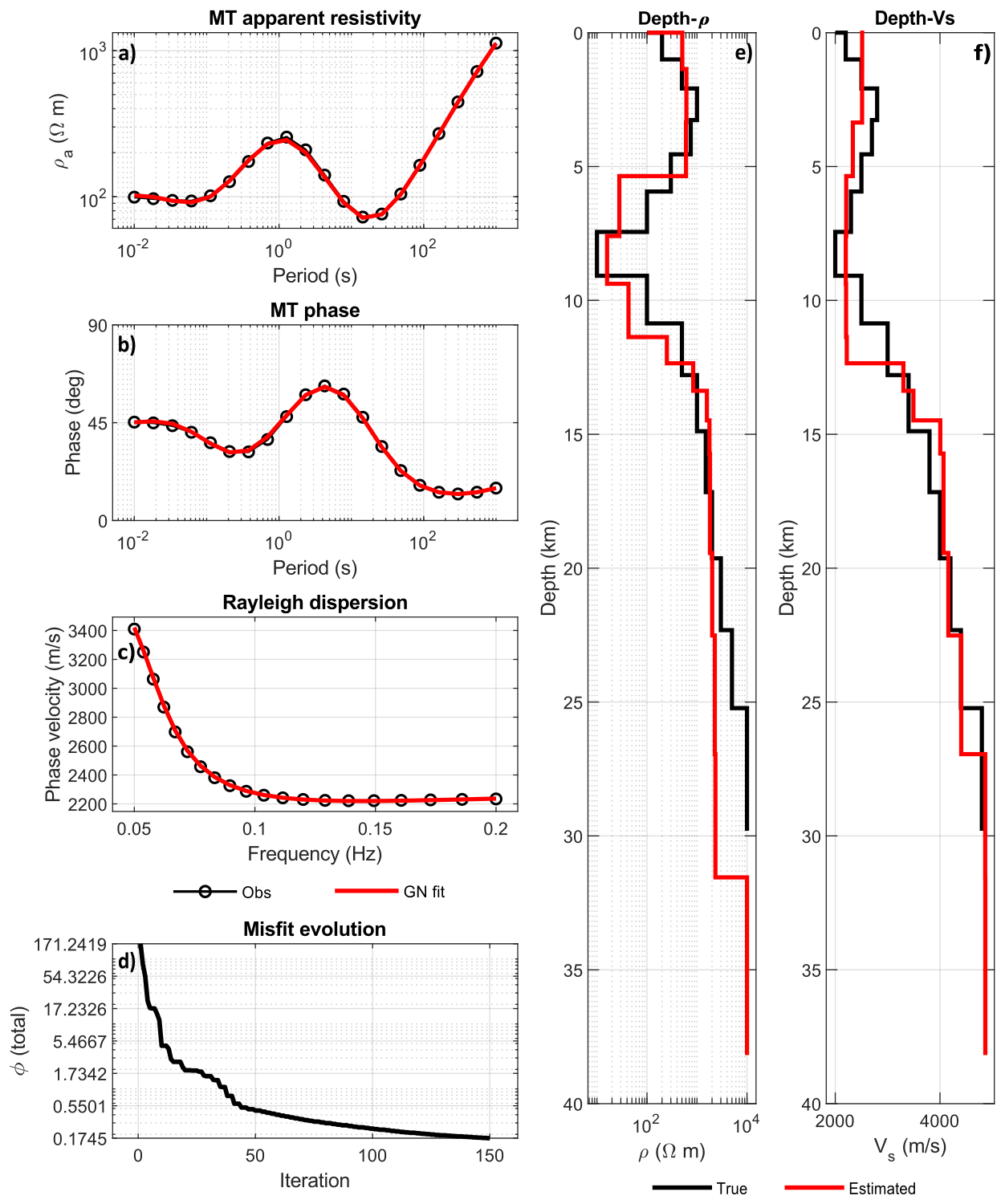
Figure 14 Results of the joint GN inversion of MT and RWD data for coupled case. (a) Apparent resistivity and (b) phase data and (c) RWD fit. (d) Total objective function over iterations. (e) ρ(z) and (f) V_s(z) models of the true and estimated models.

The misfit curve demonstrates a distinct plateau after approximately 50 iterations, indicating that the inversion has become trapped in a locally stable minimum. This behavior is consistent with the traditional inversion entering a locally stable region of model space, where further updates produce only limited reductions in misfit (Suman et al., 2010; Pallero et al., 2015; Yang et al., 2018). This is likely due to the strong dependence of gradient-based optimization on the initial model. Under the equal-weighted summation used in the GN formulation, the inversion is also forced to balance MT, RWD, and smoothness contributions within a single composite objective, so that the final solution may reflect a compromise among competing terms rather than the most representative structure for each dataset. In contrast, the Pareto–MOPSO approach avoids reliance on a single deterministic starting model and does not require the preselection of fixed relative weights between objective functions. Instead, it explores the trade-off space directly and returns a family of non-dominated solutions, thereby reducing sensitivity to local minima and providing a more transparent representation of uncertainty and inter-objective trade-offs.

All computations were performed in parallel on a 14-core CPU node (12th-generation Intel^® Core^TM i7, 2.30 GHz) with 64 GB RAM. In the Pareto–MOPSO implementation, forward evaluations were parallelized across particles in order to exploit the available multi-core resources. Both algorithms were run for 150 iterations, using the same dataset, the same forward solver, and comparable stopping criteria. In the context of the specified conditions, a single GN run necessitated 1020.70 s, whereas Pareto–MOPSO completed in 525.64 s. This outcome suggests that, for the current 1D joint inversion configuration, Pareto–MOPSO is computationally competitive and exhibits a modest advantage in terms of wall-clock time. Furthermore, in practice, obtaining a satisfactory GN solution often requires repeated trial runs to tune the initial model, relative dataset weighting, and related inversion settings. By contrast, Pareto–MOPSO reduces the need for such manual tuning by explicitly exploring the trade-off space and returning a family of Pareto-optimal solutions. This can result in significant time savings over the overall inversion workflow.

The computational cost of the Pareto–MOPSO inversion was further benchmarked by varying the swarm size P, while keeping the inversion configuration fixed at 150 iterations and using the same MT and RWD forward solvers. The measured wall-clock times for P={100, 200, 300, 400, 500} particles were {515.08, 868.82, 1218.28, 1569.85, 2025.76} s, respectively. Over this range, the runtime increases approximately linearly with swarm size, as expected, because each particle requires two forward evaluations per iteration (one MT and one RWD). For a fixed number of iterations, the total number of forward calls is therefore approximately 300 P, indicating that the runtime is dominated by forward modeling and scales close to linearly with P. A simple linear fit to the measured runtimes gives $t\approx \mathrm{3.7}P+\mathrm{1.2}\times {\mathrm{10}}^{\mathrm{2}}$ s, indicating that each increase in swarm size adds an approximately constant computational overhead. From the inversion-quality perspective, increasing P generally improves (1) the diversity and coverage of the Pareto archive, (2)  he stability of the inferred utopia solution, and (3) the interpretability of the posterior summaries (Reyes-Sierra and Coello Coello, 2006; Shu et al., 2023). This behavior is expected because a denser swarm samples the trade-off surface more uniformly within the fixed iteration budget.

The near-linear dependence on swarm size is expected to hold as long as the per-particle forward cost remains approximately constant. However, when moving from 1D layered models to 2D or 3D parameterizations, the dominant growth in computational cost is controlled not only by swarm size but also by the increasing complexity of the forward problem and the expansion of the search space. In 2D, and especially in 3D, both MT and RWD forward calculations become substantially more expensive because of larger discretizations and more demanding numerical solves. At the same time, the optimization problem becomes harder because the Pareto-optimal set should be explored in a much higher-dimensional parameter space. As a result, maintaining comparable Pareto-front quality may require larger swarms and/or more iterations, so that the total cost is expected to grow super-linearly with model dimensionality. In practice, this means that although swarm-size tuning offers a predictable cost–robustness trade-off in the present 1D framework, extensions to 2D/3D inversions will likely be constrained primarily by forward-model cost and dimensionality effects. Consequently, computationally efficient parameterizations, structural regularization, and parallel forward evaluations will be essential for preserving Pareto-front stability and uncertainty interpretability within feasible runtimes. Despite the higher computational demands in larger-dimensional problems, Pareto–MOPSO still offers a practical advantage over traditional joint inversion schemes by exploring the multi-objective trade-off space directly and reducing the need for repeated re-initializations and derivative-based tuning. Overall, the proposed workflow provides a scalable framework that is naturally suited to parallel computing for high-dimensional joint inversion problems.

7.4 Field data

Figure 15 shows the RWD curves obtained from the pairs of BOZC_paths and ECEA_paths, as well as the combined curve that best represents the phase velocities of the crustal structure along the paths between the stations using the analysis of Özalaybey et al. (2011). The period range under consideration was between 8 and 60 s; however, 8 to 20 s was employed for the modeling process in order to encompass realistic values in the crust. The RWD curves indicate a crustal structure as the seismic velocities increase with increasing period, but possible low-V_s structures can be identified as a result of the modeling phase. Figure 16 shows the MT apparent resistivities, phases and minimum phase of the phase tensor (φ_min) from the GURE and KULC stations located over the BOZC_paths and ECEA_paths, respectively. The apparent resistivity curves show a high resistivity in the first periods and a low resistivity above 1 s. The phase tensor, which is not subject to galvanic distortion in comparison to the impedance tensor (Hill et al., 2009), also exhibits a spatial variation from low to high phases, indicating high to low resistivities, as observed by Garcia and Diaz (2016) and Heise et al. (2008). However, continuous ρ(z) models can be clearly verified by the joint inversion of the datasets. Phase tensor ellipses are indicative of the fact that the MT response deviates from quasi-1D behaviour at periods which exceed approximately 1 s. At these longer periods, the ellipses become progressively more elongated, and their orientations demonstrate increased variability. This finding aligns with the concept of enhanced lateral heterogeneity and/or multidimensional effects. In order to minimize potential bias from two- or three-dimensional structure when adopting a one-dimensional inversion framework, the inversion was restricted to the short-period band (T≤1 s). In this particular band, the shapes of the phase tensors are more circular in shape and demonstrate increased stability. This period selection provides a pragmatic compromise by preserving robust information while reducing the risk of forcing multidimensional responses into a one-dimensional parameterization.

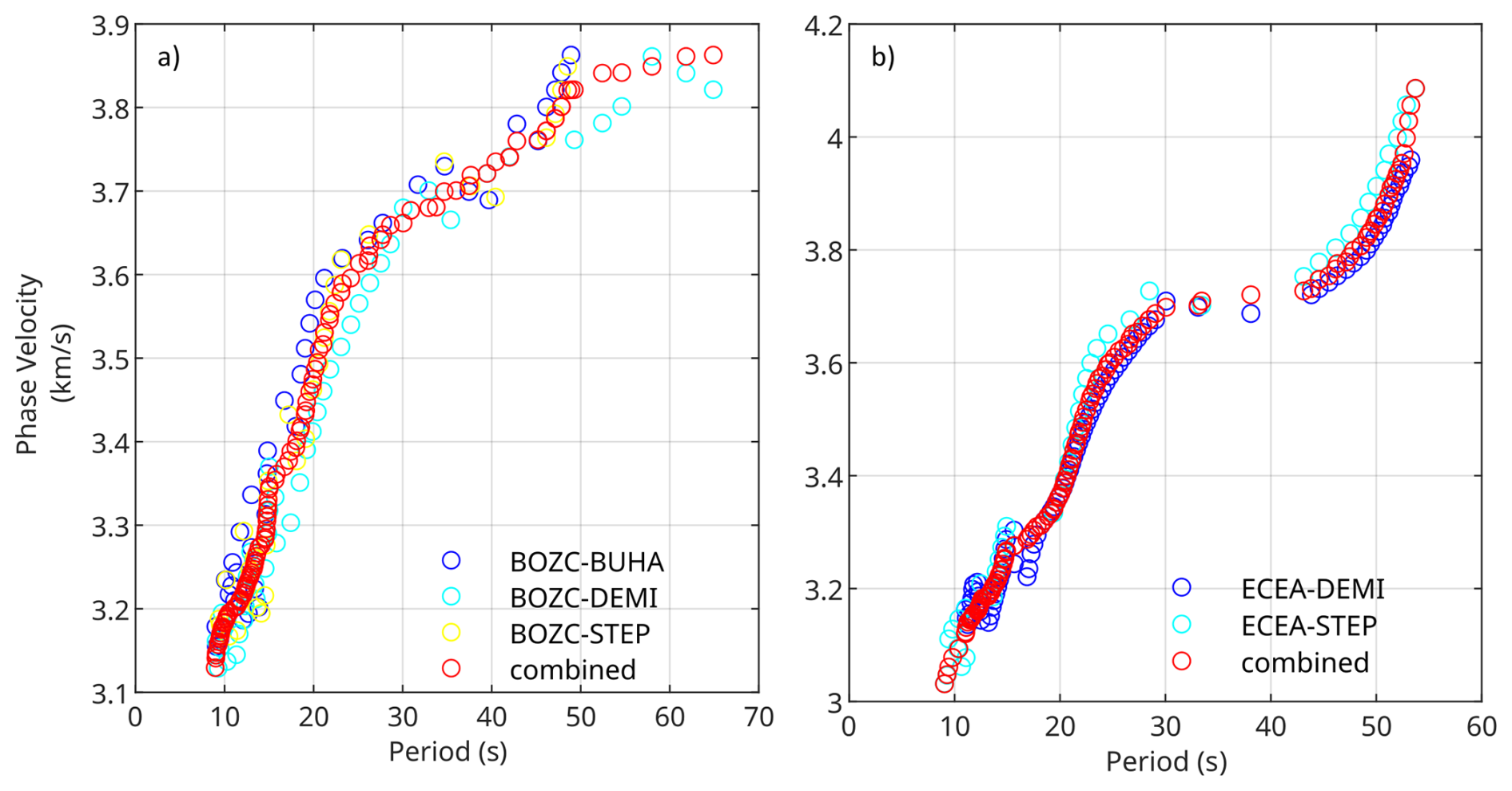
Figure 15 Measurements of an individual RWD datasets obtained from (a) BOZC_paths and (b) ECEA_paths from an earthquake with a magnitude of M_w=6.5 occurred in Italy on 30 October 2016.

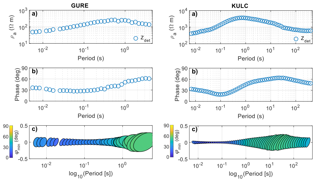
Figure 16 Measurements of individual (a) apparent resistivities, (b) phase and (c) phase tensor φ_min angles of GURE station over the BOZC_paths (left panels) and KULC station over the ECEA_paths (right panels).

Utilizing phase tensor diagnostics, the GURE MT data is constrained to a range of T≤1 s. For this specified range, the implied skin depth is estimated to be in the order of ∼8 km. The RWD data from BOZC_paths (mainly 8–20 s) primarily detects depths of ∼10–25 km (approximately $\mathit{\lambda }/\mathrm{3}$–$\mathit{\lambda }/\mathrm{2}$). Consequently, the two datasets (hereafter referred to as GBp) offer predominantly complementary constraints with minimal overlap in depth. MT primarily stabilizes the shallow resistivity structure, while RWD principally constrains the deeper V_s structure. However, the MT data from the KULC station and the RWD data from the ECEA_paths (hereafter referred to as KEp) exhibit substantially improved depth consistency in comparison with GBp. The dominant MT response at KULC is characterized by relatively high apparent resistivities (on the order of 10³–10⁴ Ωm over the short-to-intermediate period band), which implies larger electromagnetic skin depths, even at short periods. The application of the standard approximation reveals that the T≤1 s MT band at KULC corresponds to a characteristic sensitivity scale depth of ∼15–20 km. This correspondence occurs while minimizing the influence of long-period, multidimensional effects, as indicated by phase tensor diagnostics. In contrast, the ECEA RWD curve is densely sampled over a range of 8–20 s. These periods primarily sample the upper to mid-crust, situated between 10–25 km, under the assumption of crustal Rayleigh wave velocity. Consequently, the KEp datasets provide a strongly overlapping depth window between 10–25 km, enabling more physically consistent joint constraints in the parameter domain.

In the modeling stage, the 1D V_s model derived from the joint inversion is interpreted as an effective, laterally averaged structure over the propagation path/Fresnel zone, rather than as a literal point representation of the subsurface. Therefore, we do not assume that the Earth is truly 1D; rather, we extract an effective 1D model from the period band where phase-tensor diagnostics indicate quasi-1D/2D behavior and where the MT and RWD are most compatible. The purpose is to derive an effective 1D model that is commensurate with the path-averaged nature of the surface-wave dispersion data, rather than to claim a purely 1D Earth structure. This approach aligns with the established guidelines for surface-wave modeling and inversion, as outlined in the work of Foti et al. (2017). For the MT branch, the effective impedance tensor is employed to construct a 1D ρ(z) model. This model serves two purposes: it provides a physically meaningful summary of the dominant conductivity structure, and it serves as a starting point for more advanced analyses. Accordingly, first-order resistivity contrasts can be resolved and interpreted in terms of lithological variations, fluid occurrence, and/or hydrothermal alteration (Chave and Jones, 2012; Tietze and Ritter, 2013).

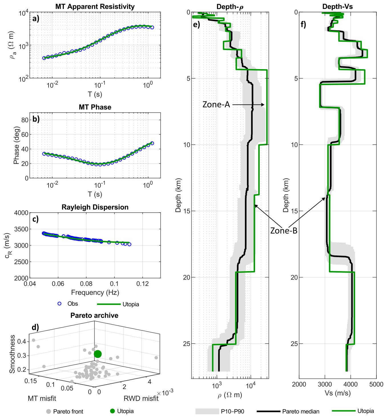
Figure 17 Representative results of the KEp. (a) Apparent resistivity, (b) phase data and (c) RWD fit with the predicted responses of the utopia solution. (d) Three-objective Pareto archive, highlighting the utopia solution. (e) ρ(z) and (f) V_s(z) models for the utopia solution, together with the P₁₀–P₉₀ envelope and the Pareto-median profile from the repository.

7.4.1 Joint modeling of the KEp

The joint MT–RWD inversions of the KEp were performed using six alternative 1D parameterizations (h=8, 12, 16, 20, 24, and 28 layers) to evaluate the impact of layer thickness and model complexity on the Pareto trade-off, data fits, and the mutual consistency of the recovered ρ(z) and V_s(z) profiles. Based on these diagnostics, we selected the 20-layer inversion (L20) as the representative field-data result (see Fig. 17). This selection was made on the basis that it provides the most balanced and interpretable joint solution. Initially, findings indicated a remarkable correspondence between MT and RWD and their observations. Secondly, the Pareto distribution is relatively compact, meaning that the utopia point does not lie at an extreme. This suggests a stable trade-off rather than objective-specific overfitting. The remaining layerings (L08, L12, L16, L24, and L28) are provided in Figs. S12–S16 to demonstrate robustness and document how under- and over-parameterization, respectively, broaden the trade-off and promote non-unique, oscillatory solutions that may weaken the physical coherence between ρ(z) and V_s(z) structures.

Across all parameterizations, the responses are generally well-reproduced at short-to-long periods/frequencies. The RWD trend is also reasonably captured, yet the extent to which a single model can satisfy both datasets simultaneously depends on the selected layering. However, the field-data layer-number comparison indicates that the MT responses are more sensitive to model parameterization than the RWD curves. While the apparent resistivity and phase fits show and improvement 8 to 20 layers and are reproduced most consistently in the 20-layer case, the 24–28-layer solutions do not provide a comparable gain. Instead, these solutions exhibit renewed systematic misfit, particularly at short-to-long periods. The Pareto archives demonstrate that low-layer parameterizations (e.g., 8 layers) produce a relatively compact but restricted trade-off structure, whereas higher-layer models (24–28 layers) become progressively more dispersed and heterogeneous, indicating increased non-uniqueness in model space. In this context, the 20-layer case provides the most balanced archive geometry, with a well-sampled yet not excessively scattered Pareto distribution and a utopia solution located within a representative part of the ensemble. The P₁₀–P₉₀ envelopes indicate that low-layer parameterizations may appear artificially narrow because of restricted model flexibility. In contrast, higher-layer cases, particularly 24–28 layers, show more heterogeneous and locally broader uncertainty, especially in the ρ(z) structure. In contrast, the 20-layer solution preserves a balanced uncertainty pattern, with sufficient ensemble variability for interpretation but without the excessive model-space dispersion associated with over-parameterization.

A focus on the preferred 20-layer solution (L20) reveals that the sensitivity partitioning between the datasets suggests that the reliability of the recovered structures is depth-dependent. In the upper crust, extending down to approximately 10 km, the MT data provide the dominant constraint, whereas the RWD data are less diagnostic of fine-scale V_s variations. Accordingly, the short-wavelength oscillations in V_s(z) within this interval are interpreted as parameterization-related artifacts rather than robust structural features. Conversely, the progressive increase in resistivity resolved by the MT data from the shallow subsurface to depths of approximately 10 km is considered as more reliable. This phenomenon aligns with the presence of a granitoid-dominated upper crust, as evidenced by previous studies (e.g., Beccaletto, 2003; Yilmaz et al., 2001). The structure exhibiting extremely high resistivity between approximately 5 and 10 km in depth is designated “Zone A”.

Below a depth 10 km, both datasets contribute structurally compatible to the joint solution. Within this depth range, the L20 models demonstrate a consistent slightly decrease in ρ, accompanied by a reduction in V_s, indicating coupled case. Therefore, the term “Zone-B” is employed to delineate a specific structure characterized by low-ρ and low-V_s with depth ranging from ∼10 to 20 km. The ρ decreases by one order of magnitude, suggesting the presence of a conductivity-enhancing phase. Meanwhile, the V_s decreases by ∼14 %, indicating a mechanically softened medium. The findings from this study are consistent with those of Turunçtur et al. (2023), who reported in V_s extending from 10 km to approximately 15–16 km in the crustal structure of the southeastern Biga Peninsula, as determined by seismic noise tomography. From an electrical perspective, the sightly decrease in ρ is most consistent with a fracture, where fault-controlled without fluid bearing enhance bulk conductivity. From a mechanical perspective, the concomitant decrease in V_s suggests a thermally weakened and/or highly cracked medium. These results are consistent with those reported by Gürer et al. (2021), who proposed that the fractured internal structure of the granitoids in the Biga Peninsula is primarily the result of changes in regional tectonic loading. As granitoid structures undergo cooling towards their bulk temperatures, brittle deformation becomes the predominant deformation mechanism. This results in the formation of a fracture, joint, and fault hierarchy whose geometry is controlled by pre-existing stress evolution (Čečys and Benn, 2007). Therefore, the co-occurrence of decreased ρ and V_s can be explained by post-emplacement deformation and fractured system increase in bulk conductivity, as well as temperature alteration. The combined effect of these factors is a reduction in elastic moduli and a decrease in V_s.

In both Zone-A and Zone-B, the utopia and Pareto-median models demonstrate a significant disparity, suggesting that these structures are susceptible to the trade-off geometry of the Pareto ensemble. This finding indicates that, while the zones are expressed in the preferred solution, their detailed amplitudes and boundary positions are not uniquely constrained and should therefore be interpreted with caution. Consequently, Zones A and B were selected for targeted sensitivity tests in the Sect. 7.4.3 to evaluate the stability of their first-order characteristics under deliberate perturbations.

At greater depths (approximately 20 km and deeper), the recovered models tend to exhibit increasing V_s while resistivity remains low or decreases and the associated P₁₀–P₉₀ envelopes widen. Given the decline in both MT and RWD sensitivities at these depths, coupled with the increasing influence of the final layers of the one-dimensional parameterization and boundary assumptions on the solution, a cautious approach is warranted when addressing these deepest-layer features. Consequently, the L20 results are interpreted as robust primarily within the depth range where the datasets provide strong, overlapping sensitivity. However, we consider any inference regarding the lower crust and Moho based on the deepest layers to be non-unique and unreliably resolved by the present joint dataset. Consequently, the recommendation is made for subsequent receiver function studies on this subject to obtain more reliable results for the lower crust and Moho.

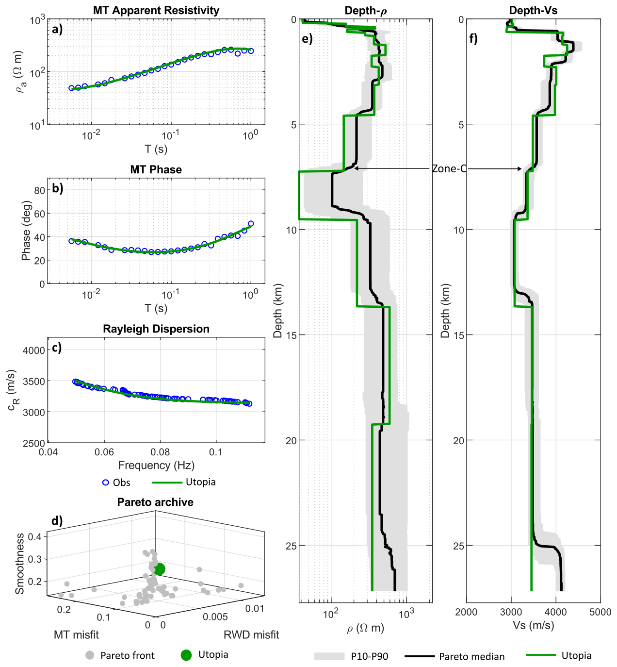
Figure 18 Representative results of the GBp. (a) Apparent resistivity, (b) phase data and (c) RWD fit with the predicted responses of the utopia solution. (d) Three-objective Pareto archive, highlighting the utopia solution. (e) ρ(z) and (f) V_s(z) models for the utopia solution, together with the P₁₀–P₉₀ envelope and the Pareto-median profile from the repository.

7.4.2 Joint modeling of the GBp

We performed joint MT–RWD inversions on the GBp field dataset using six 1D parameterizations with 8, 12, 16, 20, 24, and 28 layers. This allowed us to assess the influence of layer thickness and model complexity on the Pareto trade-off, data fits, and mutual consistency between the recovered ρ(z) and V_s(z) profiles. Based on these diagnostics, we selected the 16-layer (L16) intermediate-complexity solution as the representative field-data inversion (Fig. 18) because it provides the most balanced and interpretable joint solution. First, MT and RWD responses follow their observed trends. Second, it exhibits a relatively compact Pareto distribution, indicating a stable trade-off. The remaining layerings are provided in Figs. S17–S21.

The coarser parameterizations (8–12 layers) reproduce the first-order MT and RWD responses but tend to oversimplify the ρ(z) and V_s(z) structures, yielding smoother and less diagnostic models. In contrast, the finer parameterizations (20–28 layers) introduce additional step-like complexity and broader ensemble spread, particularly in the ρ(z) model, without a corresponding improvement in the fit curves. The 16-layer case provides the most balanced solution, as evidenced by the following: the MT apparent resistivity, phase, and RWD curves are reproduced consistently, the Pareto archive remains well organized without becoming excessively dispersed, and the depth models retain interpretable first-order structure without the over-fragmentation seen in the higher-layer cases. In addition, the P₁₀–P₉₀ envelopes indicate that the 16-layer parameterization maintains an acceptable degree of ensemble variability while avoiding the artificial narrowing associated with under-parameterization and the broader, more heterogeneous uncertainty introduced by over-parameterization.

Across all tested parameterizations, both the MT and RWD responses are reproduced reasonably well overall, indicating that the inversion captures the main observational trends in each dataset. However, with increasing parameterization, the MT fit begins to deviate systematically, whereas the RWD fit remains comparatively stable. This behavior as observed in KEp indicates that the MT responses are more sensitive to the choice of layering, and that additional model flexibility does not translate into a monotonic improvement in data-space performance. Instead, at higher layer numbers, the inversion appears to sacrifice part of the MT fit while maintaining a generally robust reproduction of the RWD curves. This finding confirms the high sensitivity of the MT branch to the data space and of the RWD branch to the model space, as we observed in the synthetic tests and KEp dataset.

Focusing on the preferred solution (L16), MT data provide the dominant constraint on ρ(z) in the upper crust (approximately to 8–10 km), whereas the RWD data are less diagnostic of fine-scale V_s variations. Accordingly, shallow short-wavelength wiggles that appear in the most complex parameterizations are interpreted as parameterization-related artifacts rather than robust structure. In contrast to the KEp, the GBp reflects the influence of continental sediments and volcanic units, consistent with its surface geological setting. Compared with the granitoid-dominated KEp, the GBp models are characterized by generally lower ρ and lower V_s (see Fig. 18). A particularly anomalous interval is observed at depths of approximately 4–10 km, where both ρ and lower V_s decrease simultaneously; this feature is here referred to as “Zone-C”. The co-occurrence of low-ρ and low-V_s is most consistently interpreted as a mechanically weak and electrically conductive upper-crustal zone.

The presence of several geothermal wells near the GÜRE station (see Fig. 6) suggests that this structure may be associated with hydrothermally altered volcanic and sedimentary units, consistent with elevated geothermal gradients and anomalous heat flow reported in previous geophysical studies (Ekinci and Yiğitbaş, 2013; Ulugergerli et al., 2007). The reservoir system develops within a complex geological framework comprising Kazdağ Group metamorphics, overlying sedimentary units, volcanic rocks, and Oligo-Miocene granitoids. In this setting, ENE–WSW-trending, south-dipping normal faults and associated fracture networks provide the main conduits for downward infiltration, deep heating, and upward discharge of thermal fluids (Akıllı et al., 2025; Sözbilir et al., 2016). From an electrical perspective, the low-ρ indicates the presence of conductivity-enhancing phases, such as interconnected saline fluids and/or hydrothermal alteration products (e.g., clay-rich assemblages) localized within a fracture network (Komori et al., 2013). From a mechanical perspective, the accompanying reduction in V_s suggests increased crack density and reduced elastic moduli, which are more consistent with a fluid-bearing, hydrothermally altered zone rather than with a melt-dominated origin at this shallow depth (O'Connell and Budiansky, 1974; Pereira et al., 2024).

Such an asymmetric decrease in ρ and V_s is also consistent with the absence of a universal relationship between these two parameters, because ρ can be strongly affected by even minor interconnected conductive phases, whereas V_s is more directly controlled by the rock matrix and its elastic framework (Bedrosian et al., 2007; Moorkamp et al., 2010). Given the hydrothermal surface manifestations in this area, the results support the interpretation of a weak and conductive crustal corridor at upper- to mid-crustal depths. However, the presence of low resistivity alone does not necessitate pervasive partial melt. A melt-related interpretation would require additional independent evidence, such as elevated $V_{\mathrm{p}}/V_{\mathrm{s}}$, strong attenuation, although Biga Peninsula associated with young magmatism (Altunkaynak and Genç, 2008; Aslan et al., 2017). In this context, Takei (2017) also showed that low-V_s and high-attenuation zones may occur near magma source regions without requiring a large melt fraction, thereby helping to reconcile inconsistencies between seismological and geochemical observations.

An additional feature of Zone-C is the pronounced separation between the utopia and Pareto-median models, particularly in the ρ(z) profile. In this interval, the utopia solution is found close to the margins of the P₁₀–P₉₀ envelope rather than near its central tendency. This indicates that the detailed expression of the conductive anomaly is sensitive to Pareto trade-off geometry. This phenomenon is analogous to that previously observed in Zones-A and -B, where the preferred solution also deviated from the ensemble median, particularly in the MT-derived resistivity structure. When considered as a whole, these patterns indicate that while the initial presence of the anomalous zone is confirmed, its precise amplitude is not uniquely defined and are sensitive to the ensemble. Therefore, Zone-C was selected as a target for sensitivity testing.

In comparison with the KEp, which manifests a coherent co-occurrence of low-ρ and low-V_s below ∼10 km, consistent with a mid-crustal weak–conductive corridor, the GBp joint inversion does not necessitate an equally pronounced low-ρ/low-V_s anomaly at the same depths. Conversely, the GBp results underscore a shallower, conductive, and mechanically weakened structure, which is consistent with active hydrothermal alteration beneath the geothermal field. This contrast is likely indicative of the varying lithological and hydrothermal regimes sampled by the two profiles. The KEp is distinguished by a granitoid upper crust, where comparatively resistive crystalline rocks are expected to prevail and high-resistivity layering effects can persist to mid-crustal depths. In contrast, the GBp crosses a more heterogeneous assemblage of continental sediments and volcanic units that commonly exhibit elevated porosity, clay-rich alteration, and fluid pathways. Consequently, the GBp models manifest systematically lower ρ and a more compliant (mechanically weakened) shallow structure. These disparities are also reflected in the absolute magnitudes and depth-dependent trends of the recovered the ρ(z) and V_s(z) distributions.

7.4.3 Sensitivity tests

To evaluate the sensitivity of the joint solution to the upper crustal high-resistivity Zone-A, and mid-crustal low-ρ and low-V_s Zone-B, we performed a targeted perturbation test in which the original utopia model was manually modified within the ∼5–10 and ∼10–20 km depth interval, respectively. In consideration of the model parameters of the layers above each zone, incremental model parameters were employed if the original model exhibited decreasing properties and vice versa. The results of the sensitivity test are presented in Figs. 19 and 20, respectively, for Zones-A and -B. We performed a sensitivity analysis to understand how variations in the input parameters affect the responses of the ρ(z) and V_s(z). Our test follows the quantitative analysis given by Garcia et al. (2015) to evaluate the quality of the data fit as follows: $\mathit{\varphi }\left(\mathit{\%}\right)=\mathrm{100}\times ({\mathit{\varphi }}_{\mathrm{m}}-{\mathit{\varphi }}_{\mathrm{o}})/{\mathit{\varphi }}_{\mathrm{o}}$, where ϕ_m is the new NRMSE of the modified model, ϕ_o is the NRMSE of the original (preferred) model. If the ϕ(%) is positive, it means a deterioration of the data fit compared to the original model. Table 1 shows the quantitative outcomes of the sensitivity tests, which involved the substitution of the original model with a modified model defined by new model parameters in each Zone-A and Zone-B.

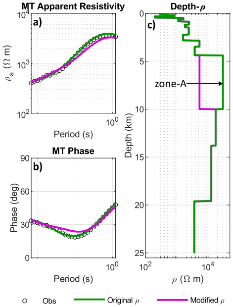
Figure 19 MT sensitivity test for the 20-layer model of the KEp. (a) MT apparent resistivity and (b) phase of the (c) modified model (magenta), obtained by replacing the ∼5–10 km high-ρ zone with low-ρ values, is compared with the original utopia solution (green).

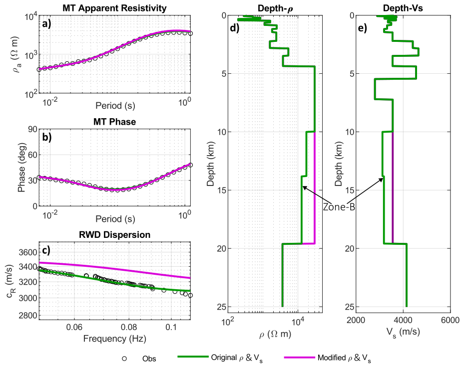
Figure 20 MT and RWD sensitivity test for the 20-layer model of the KEp. (a) MT apparent resistivity, (b) phase, and (c) RWD curves for the modified model (magenta), obtained by replacing the ∼10–20 km low-ρ zone with high-ρ values, and (d, e) for the modified model (magenta), obtained by replacing the ∼10–20 km low-V_s zone with high-V_s values, compared with the original models of the utopia solution (green).

Table 1 The sensitivity tests of Zone-A, -B and -C in the KEp and GBp solutions from updated ϕ (%) by substituting with new model parameters.

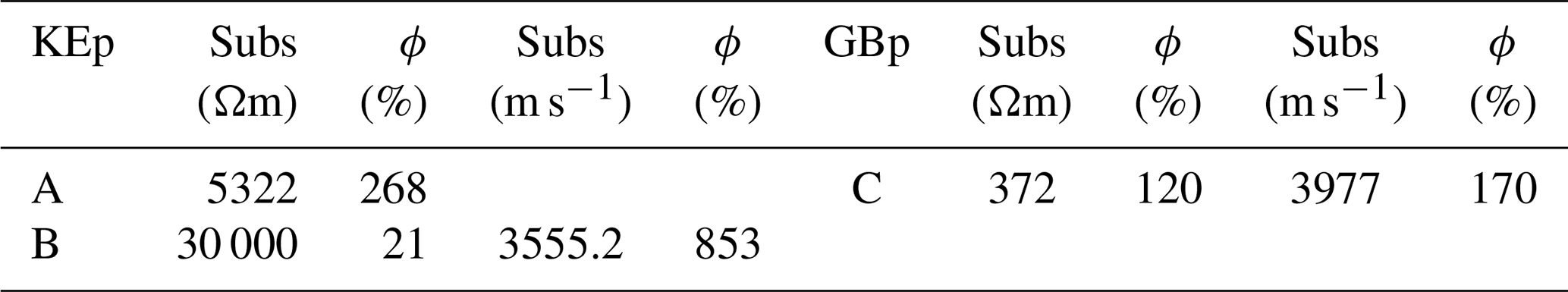
Zone-A was conducted to evaluate the role of the highly resistive zone resolved at ∼5–10 km depth in the original model (see Fig. 19). In this test, the original high-resistivity structure (∼30 000 Ωm) was replaced by a lower-resistivity continuation of the overlying unit (∼5000 Ωm). The sensitivity test shows that the imposed resistivity perturbation within Zone-A affects the MT phase most strongly at intermediate periods, whereas the apparent resistivity exhibits a broader response extending into intermediate-to-long periods. This pattern suggests that the modified layer primarily perturbs the depth-dependent transition structure sensed by the phase in its peak sensitivity band, while continuing to influence the overall impedance amplitude over a wider range of periods. The recovery of phase agreement at longer periods further indicates that the deeper bulk conductivity structure remains largely unchanged, reducing the relative impact of the Zone-A perturbation in that period range. These results support the interpretation that the presence of a highly resistive upper-crustal domain is required by the MT data, although its exact thickness and boundary geometry remain non-unique.

Table 1 show a clear degradation in the MT fit, with the logarithmic apparent-resistivity misfit increasing from 0.02 to 0.05, the phase misfit increasing from 0.72 to 2.67° and the total MT misfit increasing by ∼268 %, by the resulting forward responses. These results indicate that the highly resistive body at ∼5–10 km depth is a necessary component of the preferred MT model and is particularly important for reproducing the phase response. Accordingly, this zone is interpreted as a well-constrained and physically meaningful resistive feature rather than a non-unique artifact of the inversion. These results further confirm that the very high-resistivity structure is most plausibly related to the granitoid influence in the subsurface.

In the Zone-B experiment, the comparatively low-ρ and low-V_s structure resolved at the common depths was replaced by values closer to the more resistive and higher-velocity character of the overlying shallow crust. The outcomes of this sensitivity tests are presented in Fig. 20. In contrast to the Zone-A perturbation, the Zone-B test generates a more extensive and balanced degradation of the fit curves, suggesting that this interval is expressed collectively in both the MT and RWD datasets. In the MT responses, modification of the low-ρ structure slightly disturbs both the apparent resistivity and phase curves, particularly at the intermediate-to-long periods that are sensitive to mid-crustal depths. In addition, the RWD fit is also degraded, showing that the low-V_s component of Zone-B contributes directly to the observed dispersion behavior. The modified model predicts consistently higher phase velocities, indicating that the relatively low-V_s character of Zone-B is required by the RWD data. This behavior suggests that Zone-B is much more strongly constrained by the RWD dataset than by the MT data, and that its mechanically weakened nature is a robust feature of the preferred joint model.

As shown in Table 1, the subsequent forward responses demonstrate that the fit degradation is strongly data-type dependent. Specifically, the apparent resistivity misfit increases from 0.02 to 0.029 (∼40 %), whereas the MT phase misfit increases by only from 0.72 to 0.74 (∼3 %), indicating that the MT response is affected by this perturbation but remains comparatively less sensitive, especially in the phase data. The obtained results indicated an approximate 21 % increase in the total MT misfit (see Table 1). This behavior suggests that the presence of a mid-crustal conductive zone is less supported by the MT observations, although the exact magnitude and sharpness of the resistivity reduction are not equally constrained by all MT attributes.

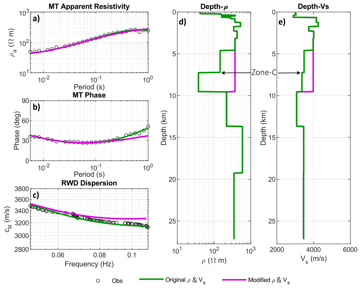
Figure 21 MT and RWD sensitivity test for the 16-layer model of the GBp. (a) MT apparent resistivity, (b) phase, and (c) RWD curves for the modified model (magenta), obtained by replacing the ∼5–10 km high-ρ zone with low-ρ values, and (d, e) for the modified model (magenta), obtained by replacing the ∼5–10 km high-V_s zone with low-V_s values, compared with the original models of the utopia solution (green).

In contrast, the RWD response exhibits a much stronger sensitivity to the same perturbation. The RWD misfit increases from 0.016 to 0.15 (approximately 8-fold), and the modified curve departs systematically from the observations over nearly the entire analyzed frequency band. Rather than producing a localized mismatch at selected frequencies, the imposed increase in V_s alters the overall dispersive behavior of the model, indicating that the low-V_s zone at ∼10–20 km depth is a first-order requirement of the RWD data. This result implies that the depth-averaged V_s(z) structure is strongly controlled by the presence of a mechanically weakened mid-crustal layer.

When considered collectively, these sensitivity results suggest that the co-located low-ρ and low-V_s anomaly in the joint inversion is not an arbitrary artifact of the parameterization, but rather a physically meaningful component of the preferred model. However, it is important to note that the two datasets do not impose equivalent constraints on Zone-B. The RWD data impose a significantly more stringent constraint on the existence of the low-V_s zone, whereas the MT data also support an associated conductive region but allow comparatively greater flexibility. The joint solution thus supports the interpretation of a weak and conductive mid-crustal corridor, with the seismic data providing the strongest evidence for its persistence and the MT data independently reinforcing its electrically anomalous character. The sensitivity test indicates that the observed anomaly may be attributed to a fault-controlled, highly fractured, and thermally weakened granitoid domain.

The outcomes of the GBp sensitivity is presented in Fig. 21. In this test the low-ρ and low-V_s structure identified as Zone-C at approximately 5–10 km depth was replaced by the overlying high-ρ and high-V_s unit. This modification leads to a pronounced deterioration of the joint data fit, thereby confirming that Zone-C is a required and robust component of the original model. Quantitatively, the apparent resistivity misfit increases only slightly from 0.05 to 0.06, whereas the phase misfit rises much more strongly from 1.15 to 4.13, resulting in an overall increase of about 120 % in the total MT misfit. This contrast indicates that the MT phase response is considerably more sensitive than apparent resistivity to the presence of Zone-C. In particular, the phase curves diverge progressively toward longer periods, while the apparent resistivity response remains comparatively closer to the observations, implying that the conductive nature of Zone-C is expressed more clearly in the phase behavior than in the amplitude response alone.

The RWD response also degrades substantially following this modification. The RWD misfit increases from approximately 0.023 to 0.065, corresponding to an increase of about 1.7-fold, and the RWD curve begins to separate from the original solution already at the high-frequency end, with the mismatch persisting into the intermediate-frequency range. This behavior indicates that Zone-C is also required to explain the shallow-to-intermediate depth shear-wave structure sampled by the RWD data. Accordingly, although the anomaly is most strongly demanded by the MT phase response, it is also independently supported by the RWD observations.

Taken together, these results offer an independent validation of our interpretation of Zone-C. From an electrical viewpoint, the strong sensitivity of the MT response confirms that the low-ρ is not incidental. Rather, it reflects the presence of conductivity-enhancing phases, such as interconnected saline fluids and/or hydrothermal alteration products (e.g., clay-rich assemblages) localized within a fracture-controlled network. From a mechanical viewpoint, the substantial degradation in the RWD fit after removal of the low-V_s interval provides support for the interpretation that Zone-C is characterized by increased crack density and reduced elastic moduli. Therefore, the sensitivity analysis thus corroborates the conclusion that Zone-C represents as a fluid-bearing, hydrothermally altered weak zone, rather than a compact a melt-dominated source at this shallow crustal level.

8 Conclusions

This study demonstrates the application of Pareto–MOPSO for the joint inversion of MT and RWD data characterized by fundamentally different physical sensitivities and lacking a universal petrophysical relationship. Through systematic testing on synthetic and field data from two sites in the southeastern Biga Peninsula, we investigated the behavior of coupled and decoupled parameterizations, noise sensitivity, and layering configurations to assess the robustness and practical utility of the multiobjective framework. Despite the absence of a universal empirical law linking electrical resistivity and seismic velocity, the Pareto–MOPSO approach successfully recovered subsurface models. The Pareto front and associated statistical metrics (median, P₁₀–P₉₀ percentiles) provided meaningful insights into both the trade-offs between competing data types and the uncertainties inherent in each parameter space. The Pareto-median model emerged as a robust representative of the non-dominated ensemble, effectively capturing the general trends in subsurface structure rather than representing a single “true” Earth model. The P₁₀–P₉₀ envelope quantified parameter uncertainty across the model space, offering a transparent measure of solution variability.

Layering sensitivity tests revealed that the main recovered features remained stable within the uncertainty bounds, and the position of the knee-point solution on the Pareto front did not change materially with modest variations in layer configuration. This stability underscores the reliability of the method in capturing first-order subsurface structure even when layer discretization is not perfectly known a priori. A particularly significant finding of this study is the distinct divergence between data-space sensitivity and model-space uncertainty under increasing noise levels. Noise sensitivity tests confirm that the MT branch remains more vulnerable to parameter trade-offs under the shared thickness parameterization, being more sensitive in the parameter space, while RWD is more sensitive to perturbations in the data space.

Application to field data from the southeastern Biga Peninsula yielded models that are compatible with known geological formations at certain depths. The obtained results indicate that joint inversion is capable of resolving compatible conductive and mechanically weak domains at different crustal levels. While their geological controls may differ in detail, their coupled signatures consistently point to reduced elastic moduli and enhanced bulk conductivity associated with fracturing, thermal modification, and locally hydrothermal processes. However, the compatibility could be improved if the datasets exhibited stronger mutual constraints at overlapping depth ranges. Therefore, the present results should be regarded as providing only a rough overview of the crustal structure in the study area, as the focus of this work was on demonstrating the practicality of Pareto–MOPSO for joint modeling. A comprehensive crustal-scale interpretation utilizing additional datasets and higher-dimensional modeling is beyond the scope of this study but represents a promising avenue for future work.

Although this study employed one-dimensional models, the Pareto–MOPSO framework offers significant advantages for 2D and 3D joint inversion of MT and RWD data. In such cases, the parameter space becomes high-dimensional, and traditional derivative-based methods (e.g., Gauss–Newton algorithms) encounter challenges related to initial model dependence, relative weighting schemes, and manual tuning. Pareto–MOPSO explicitly explores trade-offs in a multiobjective space and reduces the need for manual tuning of initial models, data weighting, and regularization parameters.

The findings of this study encourage to consider Pareto–MOPSO for joint geophysical inversion, particularly when: (1) multiple datasets with different physical sensitivities are available; (2) no universal petrophysical relationship exists between the measured properties; (3) quantification of trade-offs and uncertainties is essential for interpretation; (4) high computational capacity is accessible to handle the population-based optimization. Future work should extend the methodology to 2D and 3D geometries, incorporate additional geophysical datasets (e.g., gravity, seismic refraction), and explore adaptive parameterization schemes. Furthermore, integration with geological and petrophysical constraints could help narrow the solution space and enhance the interpretability of the Pareto-optimal ensemble.