Sandy beaches' chaos: shoreline-sandbar coupling inferred from observational time series

Sandy shoreline–sandbar systems exhibit complex variability arising from the interplay between hydrodynamic forcing and intrinsic morphological feedbacks. Using long-term satellite-derived shoreline and sandbar observations, we applied global polynomial modeling to reconstruct low-dimensional deterministic dynamics for 4 contrasting coastal sites. The resulting autonomous models reproduce key morphodynamic features, including self-sustained shoreline oscillations, shoreline–sandbar coupling, and intermittent transitions between quasi-stable configurations. Nonlinear stability analyses reveal that these systems behave as chaotic oscillators, characterized by locally divergent yet globally bounded trajectories. Energetic episodes correspond to rapid shoreline–sandbar exchanges, whereas long low-energy states reflect stable attractor confinement. Together, these results demonstrate that sandy coasts are governed by deterministic but chaotic dynamics, in which internal coupling and self-organization control both variability and finite predictability. The proposed framework offers a physically consistent and data-driven approach to characterize and compare coastal morphodynamics within a unified nonlinear dynamical perspective.

1 Introduction

Systems in geosciences are inherently complex, nonlinear, and often display sensitivity to initial and boundary conditions, leading to behaviors that range from approximately quasi-periodic or near-periodic oscillations (Chazallon, 1842; Bell, 1962; Pekeris and Accad, 1969; Cartwright, 2000; Durand-Richard, 2016) to low-dimensional chaos (Lorenz, 1963; Nicolis and Nicolis, 1991; Maas and Doelman, 2002; Sévellec and Fedorov, 2014; Mosto et al., 2024b; Charó et al., 2025) and high-dimensional stochastic-like dynamics (Jin et al., 1994; Dijkstra, 2013; Vallis, 2017). Such systems are typically governed by the interplay between internal feedbacks and external forcing (Ghil and Sciamarella, 2023; Di Capua et al., 2023; Maraldi et al., 2025), operating across multiple spatiotemporal scales (Lovejoy, 2019). For example, the ocean–atmosphere system can exhibit a high sensitivity to initial conditions (Penduff et al., 2018; Waldman et al., 2018; Jamet et al., 2019; Cravatte et al., 2021), while river deltas, dune fields, and coastal morphodynamics all exemplify nonlinear organization, where irregularity coexists with underlying low-dimensional dynamics (Baas, 2002; Coco and Murray, 2007; Murray et al., 2009; Jerolmack and Paola, 2010; Murray et al., 2014). In particular, coastal environments represent a natural laboratory for studying nonlinear self-organization under continuous external forcing, as they integrate hydrodynamic energy input (waves, tides, sea level anomalies), sediment transport, and morphological feedback loops within a dynamically evolving boundary system (Castelle and Masselink, 2023).

Recent advances in satellite Earth observation now make it possible to monitor coastal morphology at unprecedented spatiotemporal scales (Luijendijk et al., 2018; Vos et al., 2020, 2023; Konstantinou et al., 2023; Almar et al., 2023; Castelle et al., 2024; Graffin et al., 2025; Frugier et al., 2026). Time series of shoreline and active nearshore sandbar positions can be extracted from optical satellite imagery, enabling continuous monitoring of beach morphology over decadal timescales with weekly to monthly resolution. These remote sensing observations have now been extensively validated against in-situ field surveys at several historical sites for shoreline data (Vos et al., 2023; Graffin et al., 2025); similar for sandbar data (Tătui and Constantin, 2020; Frugier et al., 2025, 2026), demonstrating their capacity to resolve the coevolution of the shoreline-sandbar system. The resulting datasets provide, for the first time, sufficiently long and coherent records to analyze the internal dynamics of beach systems.

In parallel, data-driven modeling approaches have emerged as a powerful complement to process-based models for exploring the dynamics of complex systems (Crutchfield and McNamara, 1987; Gouesbet, 1991; Gouesbet and Letellier, 1994; Aguirre and Billings, 1995; Mangiarotti et al., 2012; Brunton et al., 2016; Somacal et al., 2022; Omejc et al., 2024; Guo et al., 2025; Simmons and Splinter, 2025). Among these and derived from the theory of non-linear dynamical systems, the global modeling technique aims to reconstruct deterministic dynamical systems directly from observational time series, without making strong assumptions about predefined governing equations, and has shown promising results from both synthetic (Gouesbet and Letellier, 1994; Aguirre and Letellier, 2009; Letellier et al., 2009; Mangiarotti and Huc, 2019), experimental (Letellier et al., 1995) and real world data (Boudjema et al., 1995; Maquet et al., 2007; Mangiarotti et al., 2016; Mangiarotti and Le Jean, 2023). More broadly, the objective of inferring interpretable governing equations directly from data has recently attracted increasing attention, with the development of equation-discovery frameworks such as symbolic regression approaches (Schmidt and Lipson, 2009) and sparse identification techniques, including SINDy (Brunton et al., 2016; Rudy et al., 2017), as well as methods such as GPoM (Mangiarotti et al., 2012; Mangiarotti and Huc, 2019), proGED (Brence et al., 2021), and L-ODEfind (Somacal et al., 2022). These methods all similarly seek parsimonious representations of the underlying dynamics based on observations by selecting a small set of active terms from a library of candidate nonlinear functions. At present, few of them enable obtaining interpretable dynamical equations from environmental time series (e.g. in eco-epidemiology (Mangiarotti, 2015)), and this remains a challenging problem (Song et al., 2024).

One of the few existing frameworks offering a semi-automated implementation of the global modeling approach is the Global Polynomial Modeling (GPoM) package (Mangiarotti et al., 2012). Developed in R, this package integrates a suite of algorithms designed to reconstruct low-dimensional deterministic systems directly from time series. GPoM identifies parsimonious polynomial equations capable of reproducing the observed phase-space geometry and attractor structure by iteratively selecting the minimal subset of nonlinear terms that preserves the variance and structural properties of the reconstructed trajectories. This procedure provides an interpretable representation of the underlying feedbacks and coupling mechanisms between variables involved, and enables testing for deterministic structure within empirical dynamical systems. Such an approach is particularly relevant given that inferring the underlying dynamics of chaotic geophysical systems from noisy and incomplete observations remains a fundamental challenge in the environmental context characterized by low predictability (Jardak and Talagrand, 2018; Ruiz et al., 2022).

In this study, we apply GPoM to a multi-site dataset of satellite-derived shoreline and sandbar time series, representing diverse morphodynamic contexts along wave-dominated coasts. We show that, despite differences in local forcing and sedimentary setting, these systems exhibit a common dynamical structure characterized by nonlinear coupling between the shoreline and the sandbar. The recovered equations capture the essential features of the observed oscillations and reveal a regime of chaos, in which the system remains bounded but sensitive to perturbations. Furthermore, by comparing the reconstructed feedback loops across sites, we propose a preliminary typology of shoreline-sandbar systems, depending on their coupling direction and mechanisms. These results suggest that low-dimensional nonlinear models can provide an interpretable framework for understanding and classifying beach internal dynamics.

The remainder of the paper is structured as follows. Section 2 describes the dataset and the methodology for GPoM usage. Section 3 presents the models assessment and physical interpretation. Section 4 discuss the results implications. Section 5 summarizes the main conclusions and outlines future research perspectives.

2 Methods

2.1 Dataset

2.1.1 Satellite images

The Python API of Google Earth Engine (GEE) was used to download satellite images, providing access to publicly available top of atmosphere reflectance images (Level-1C) from various collections (Chander et al., 2009; Gorelick et al., 2017). Sentinel-2 images with a 10 m resolution and 5 d revisit time were downloaded for the 4 sites: Torrey Pines, Ensenada, Duck and Gold Coast. The blue (B), green (G), and red (R) bands corresponding to visible light wavelengths, the Near-InfraRed (NIR) band just beyond visible red, and the Short-Wave InfraRed (SWIR1 and SWIR2) bands covering longer wavelengths beyond NIR, were downloaded. Bicubic interpolation was applied to the SWIR1 and SWIR2 bands, which originally have a 20 m resolution and are resampled to 10 m resolution like the other bands. To further refine the data quality, a cloud cover threshold was applied using GEE's built-in tools. However, this threshold applies to the entire satellite image tile, which may result in rejecting images that are cloud-free in the Region Of Interest (ROI). To address this issue, all images with total cloud cover below 90 % were included in our analysis, and a custom function developed by Graffin et al. (2025) was applied to filter out images with cloud cover specifically within the ROI.

2.1.2 Satellite-derived shoreline position

The shoreline is detected and extracted using the method developed by Bergsma et al. (2024), specifically designed for sandy beaches, with root mean scare error typically below 10 m. This approach combines a multi-spectral index, the Subtractive Coastal Water Index (SCoWI) with Otsu's threshold refinement method and Marching Squares algorithm to derive sub-pixel shoreline positions (Otsu, 1979; Cipolletti et al., 2012) as:

$$\begin{array}{}\text{(1)}& \begin{array}{rl}\text{SCoWI}=& B+\mathrm{2}\times (G-\text{NIR})-\mathrm{0.75}\times \text{SWIR1}\\ & -\mathrm{0.5}\times \text{SWIR2}\end{array}\end{array}$$

where B, G, NIR, SWIR1 and SWIR2 represent the reflectance values of the respective spectral bands: blue, green, near-infrared, short-wave infrared 1 and 2. The shoreline proxy corresponds to the waterline, which reflects variations in sea level including minor tidal effects, as well as other sea-level fluctuations occurring across different timescales.

2.1.3 Satellite-derived sandbar position

Few studies use satellite images to detect sandbars. Up to date, there are primarily manual extraction approaches (Rodríguez-Martín and Rodríguez-Santalla, 2013; Athanasiou et al., 2018); while automatic methods remain rare in the literature (Tătui and Constantin, 2020; Janušaitė et al., 2021). Aside from the work of Frugier et al. (2025) and Tătui and Constantin (2020), both relying on satellite images, no other study, to date, addresses the automatic extraction of sandbar positions using publicly available high-resolution satellite data such as Sentinel-2 or Landsat. Unlike the shoreline, sandbars are submerged features and cannot be directly observed. However, their presence induces wave breaking when incident waves are energetic enough to shoal and dissipate over the bar. The resulting foam pattern provides a visual signature that can be used to infer the sandbar position. Lippmann and Holman (1989) were the first to exploit video imagery to track sandbar positions through time-averaged sequences (time-exposures). Similarly, following the principle of the SCoWI index developed for shoreline detection, the SandBar Index (SBI) proposed by Frugier et al. (2025) automatically identifies and extracts sandbar positions by maximizing the contribution of high-intensity (breaking) pixels while minimizing contributions from other environments (land, sand, and water), with reported root mean square error on the order of 20 m, corresponding to approximately two Sentinel-2 pixels (see, e.g., the SBI framework). However, because the different satellite missions used in this study (e.g., Landsat, VENµS, Sentinel-2) cover distinct radiometric ranges and sensor-specific reflectance characteristics, we introduced a normalized version of the index (NSBI) to ensure methodological consistency and cross-sensor comparability throughout the monitoring period and across all study sites. This normalization allows the reliable detection of breaker zones in satellite imagery and the estimation of sandbar positions through wave-breaking patterns:

$$\begin{array}{}\text{(2)}& \text{SBI}=\mathrm{2}\times (B-R)+G+\mathrm{0.25}\times \text{NIR},\end{array}$$

and:

$$\begin{array}{}\text{(3)}& \text{NSBI}={\displaystyle \frac{\text{SBI}-{\text{SBI}}_{min}}{{\text{SBI}}_{\mathrm{90}}-{\text{SBI}}_{min}}}\end{array}$$

Normalization is applied using the 90th percentile of the data rather than the absolute maximum to remove outliers influence, such as excessive reflections or sensor errors, which do not represent typical conditions. A threshold of NSBI > 1.2 allows the identification of breaking zones within a given region of interest and has been shown to be valid across different sites and satellite missions (Frugier et al., 2025, 2026).

2.1.4 Transects

Transects were manually constructed within QGIS framework (QGIS Development Team, 2025) by first drawing a baseline along the landward edge of the beach, following its shape, and then generating perpendicular transects directed seaward with origin on land and spaced 30 m apart with lengths adapted to each beach.

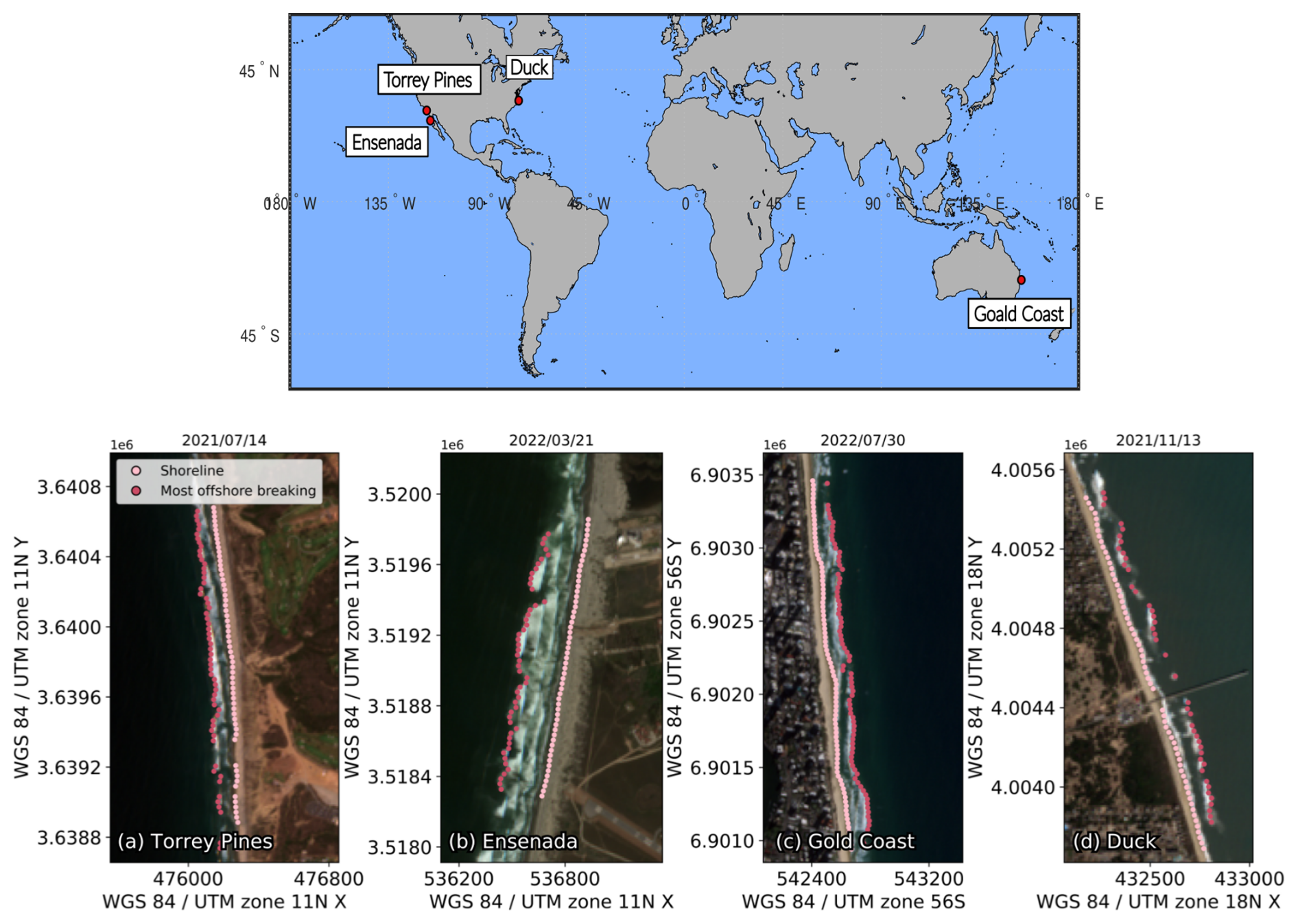
Figure 1 Study sites locations along with illustrative snapshot of the shoreline and sandbar detection via satellite imagery. Each beach is presented on a specific date: (a) Torrey Pines (14 July 2021), (b) Ensenada (31 March 2022), (c) Gold Coast (30 July 2022), and (d) Duck (13 November 2021). Imagery © 2022 CNES/Airbus, Map data © 2022 Google.

2.1.5 SDS and SDSb time series

Waterlines were projected onto the cross-shore transects and the shoreline position x_s was measured along each transect relative to its land origin. The mean shoreline position $\stackrel{\mathrm{‾}}{x_{\mathrm{s}}}$ across all transects was then estimated for each satellite image, producing the Satellite-Derived Shoreline (SDS) time series. Breaking lines were projected onto the same transects, and the breaking position x_b was measured relative to the land origin. As wave breaking is instantaneous, its spatial pattern can differ between transects. On single-bar beaches, some transects show breaking over the bar while others do not; on double-bar beaches, breaking may occur at the inner bar and/or at the outer bar (Wright and Short, 1984). To consistently identify the offshore breaking associated with the bars, K-means clustering was applied along the cross-shore axis. Only well-separated clusters (silhouette score > 0.65) were retained. Within each reliable cluster, breaking positions were extracted, and the offshore cluster was selected. When clustering was unreliable, a single breaking line was assumed. The mean sandbar position $\stackrel{\mathrm{‾}}{x_{\mathrm{b}}}$ across all transects was then computed for each satellite image, capturing the representative active sandbar position. Clusters were considered valid only if at least 20 % of transects exhibited breaking; otherwise, they were discarded and the next well-separated offshore cluster was evaluated in the same way. The resulting Satellite-Derived Sandbar (SDSb) time series therefore reflects the typical offshore breaking position associated with sandbars. The time series start just before 2018 as between 2015 and 2018, only Sentinel-2A was operating, providing very sparse data.

Figure 1 shows the geolocation of the 4 sites along with Sentinel-2 images highlighting the detection of the shoreline (x_s, light pink) as well as the submerged active sandbar (x_b, offshore breaking, dark pink) along the transects for each beach on a specific date.

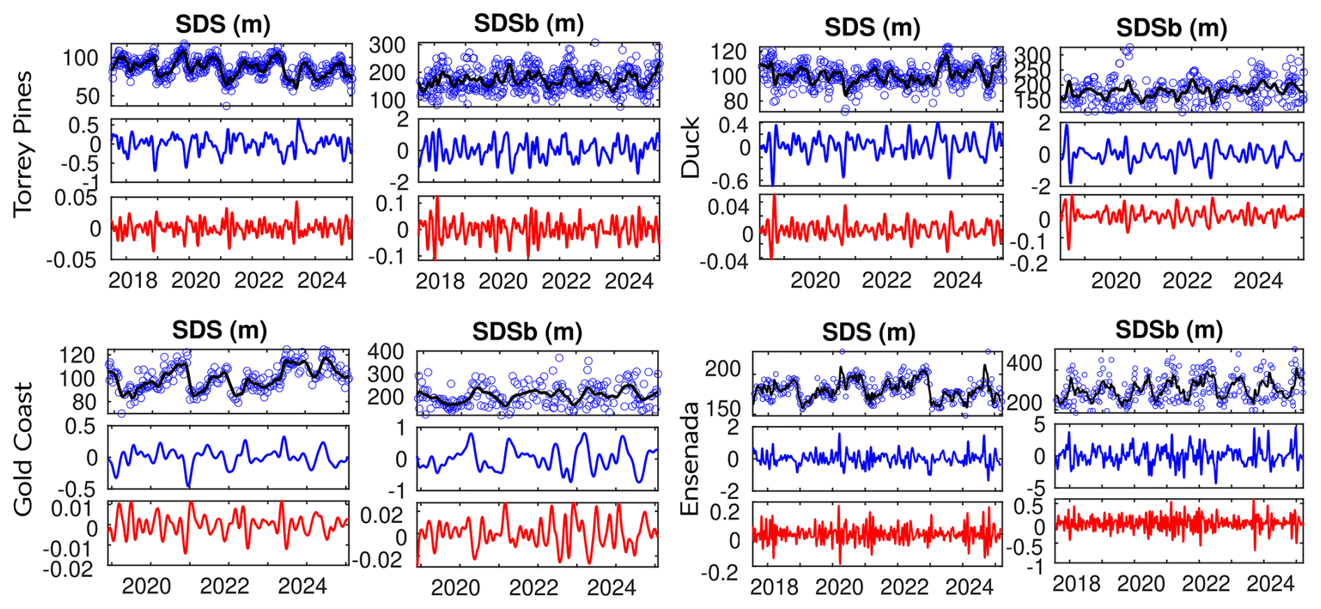
Figure 2 Study sites time-series overview. Satellite-derived shoreline (SDS) and nearshore sandbar (SDSb) time series and their first- and second-order temporal derivatives (blue and red, respectively) for the 4 study sites: Torrey Pines (USA), Gold Coast (Australia), Ensenada (Mexico) and Duck (USA). Raw daily observations (blue dots) and smoothed trajectories (black lines) are shown together with the corresponding time derivatives computed using a Savitzky–Golay filter.

2.2 Sites overview

The 4 study sites capture a range of morphodynamic conditions along wave-dominated sandy coasts: Torrey Pines (California, USA) is a medium-grained barred beach (D₅₀≈ 0.2 mm) backed by steep cliffs and influenced by complex wave refraction from offshore islands (Ludka et al., 2019). Yearly-averaged significant wave height conditions are H_s≈ 1–1.5 m with peak periods of T_p≈ 10–12 s. Ensenada Beach (Baja California, Mexico) is an intermediate mesotidal system with a single active sandbar (D₅₀≈ 0.25 mm) responding to a bimodal swell regime: energetic north-westerly winter waves (H_s up to 4 m) and milder south-westerly summer waves (H_s≈ 0.7 m) (Ruiz De Alegría-Arzaburu and Vidal-Ruiz, 2018). Duck (North Carolina, USA) is a double-bar beach exposed to high-energy Atlantic forcing (H_s≈ 1.2–1.8 m, T_p≈ 8–10 s) exhibiting strong seasonal variability in sandbar dynamics (Lippmann and Holman, 1990). Gold Coast (Queensland, Australia) is a double-barred quartz-sand beach (D₅₀≈ 0.25 mm) exposed to persistent south-easterly swells (H_s≈ 0.8 m, T_p≈ 9–10 s) and an intense northward littoral drift of about 5 × 10⁵ m³ yr⁻¹ (Price et al., 2011).

Together these sites encompass the principal morphodynamic regimes described by Wright and Short (1984) and Masselink and Short (1993): from micro- to mesotidal, single- to double-bar, and reflective to dissipative states, forming a coherent natural laboratory for analyzing shoreline–sandbar coupling.

2.3 Data preprocessing

To account for local 3D-variability, we computed the mean shoreline and sandbar positions ($\stackrel{\mathrm{‾}}{x_{\mathrm{s}}},\stackrel{\mathrm{‾}}{x_{\mathrm{b}}}$) across all available transect using a robust interquartile range (IQR) estimator (Whaley III, 2005), which mitigates the influence of outliers and ensures stability in the composite signal, particularly during energetic events or data gaps. Because satellite-derived shoreline and nearshore sandbar positions exhibit different levels of noise, typically higher for the sandbar as the variability of offshore breaking is much more sensitive to stochastic day-to-day variations in wave forcing, temporal smoothing windows were individually adjusted to retain intra-seasonal to interannual variability (typically 1–3 months smoothing) while filtering out high-frequency noise. The resulting time series were then standardized (zero mean, unit variance) and resampled onto a common daily grid using spline interpolation to ensure continuous and smooth first- and second-order temporal derivatives, yielding a single representative time series for shoreline and sandbar positions at each site (Fig. 2).

2.4 Global modeling using GPoM

The global modeling approach provides a fully data-driven framework to retrieve a minimal set of ordinary differential equations (ODEs) capable of reproducing, from observations, both the temporal trajectories (over short timescales) and the set of states toward which the system evolves over time, without prior assumptions about the underlying physical processes (Mangiarotti and Huc, 2019).

2.4.1 Concept and theoretical background

According to the embedding theorem of Takens (1981), the dynamics of a deterministic system can be reconstructed from a limited number of observables by using either delays, time derivatives, or a combination of both (Sauer et al., 1991), provided that the embedding dimension is sufficiently large and the observability of the variables (i.e. the amount of information about the system dynamics contained in each observable) is sufficiently high (Aguirre et al., 2018; Letellier et al., 2018). Global modeling exploits this principle to infer the functional form of the governing equations as:

$$\begin{array}{}\text{(4)}& {\displaystyle \frac{\mathrm{d}{X}_i}{\mathrm{d}t}}=\sum _{j=\mathrm{1}}^{N_{\mathrm{p}}}{K}_{ij}{\mathrm{\Phi }}_j(X_{\mathrm{1}},X_{\mathrm{2}},\mathrm{\dots },X_m),i=\mathrm{1},\mathrm{\dots },m,\end{array}$$

where X_i denotes the ith state variable (with m the total number of variables), ${\mathrm{\Phi }}_j(X_{\mathrm{1}},X_{\mathrm{2}},\mathrm{\dots },X_m)$ denotes the jth polynomial monomial constructed from the state variables up to degree d_max (e.g., $X_{\mathrm{1}}^{\mathrm{2}}$, X₁X₂, $X_{\mathrm{2}}^{\mathrm{3}}$, etc.), forming the functional basis of the model, and K_ij the coefficients estimated by linear regression. Each equation thus represents the temporal evolution of 1 variable as a polynomial combination of all others.

In practice, time derivatives of the observables are estimated through Savitzky–Golay filtering, which preserves local polynomial consistency and minimizes noise amplification in comparison to finite-difference schemes (Ahnert and Abel, 2007). The resulting derivatives (Fig. 2) form the basis for constructing candidate differential equations, which are then combined into a full dynamical system.

2.4.2 Implementation in the GPoM package

The GPoM package (Mangiarotti et al., 2012; Mangiarotti and Huc, 2019) implements this approach in R and provides a semi-automated framework for model discovery, selection, and validation. It systematically explores combinations of polynomial terms given the number of state variables m, the maximum polynomial degree d_max, and the maximum derivative order. Each candidate model is numerically integrated and compared with observations using statistical and geometric criteria such as variance preservation, correlation between observed and simulated variables, as well as structure reliability of the reconstructed attractor in the phase space.

By iteratively selecting the most informative, dynamically consistent, and parsimonious subset of terms, GPoM builds low-dimensional polynomial models that capture the essential nonlinear coupling and feedback mechanisms among variables (Mangiarotti et al., 2025). These models can then be used to investigate the deterministic structure of the system, assess its stability properties, and explore potential bifurcations or chaotic regimes emerging from the coupled dynamics.

In this study, GPoM is applied to the coupled evolution of shoreline and active sandbar systems. The objective is to identify minimal polynomial models capable of reproducing the observed phase-space geometry and the dynamical interplay between shoreline position and sandbar migration, thereby revealing the feedbacks governing coastal morphological variability.

2.5 Protocol

In order to explore system complexity and potential chaos, model dimensions m=3 and m=4 were tested within GPoM, with polynomial degree ranging from $d_{max}=\mathrm{2}$ to 4. According to the Poincaré–Bendixson theorem, continuous autonomous systems of dimension m≤2 can only display a very low level of complexity, as their trajectories are confined to fixed points or period-1 limit cycles (Poincaré, 1893), thus precluding the stretching and folding dynamics required for chaos (Gilmore and Lefranc, 2002). Hence, higher-dimensional embeddings (m≥3) were explored to enable the capture of complex feedbacks and non-trivial oscillatory regimes. All possible variable combinations among $(X_{\mathrm{1}},X_{\mathrm{2}},X_{\mathrm{3}},X_{\mathrm{4}})$ satisfying m=3 or 4 were systematically explored after truncating 100 d from both ends of the time series to minimize edge effects associated with smoothing and derivative estimation. Each final model was thus inferred from approximately 95 % of the total record length (∼ 10 years of Sentinel-2 revisits), which, in cases where robust deterministic models were obtained, provides strong evidence for determinism within the real-world data dynamics. A moving window of ω = 51 d was used for derivative smoothing using the Savitzky–Golay filter. Sensitivity tests around this window size showed no significant change in the resulting model structure, confirming the robustness of the reconstruction. The number of polynomial terms K (Eq. 4) allowed in the models was set between K=6 and K=26, covering a broad range of configurations while limiting overfitting due to excessively complex models. Finally, candidate models that were neither fixed points nor simple limit cycles and remained numerically stable for at least 80 years of integration were visually inspected. Model quality was primarily assessed through phase-space consistency and amplitude preservation rather than pointwise prediction accuracy, as GPoM aims to reproduce the system's underlying geometry rather than forecast individual states. Among these, the most parsimonious model (i.e., the one with the smallest combination of K, m, and d_max) was retained for further dynamical analysis. As explicitly stated, the embedding dimension was not fixed a priori through classical diagnostics such as false nearest neighbors for several reasons: (i) our objective is to obtain an interpretable low-dimensional approximation of the observed dynamics; (ii) the original time series are noisy, and it is difficult to distinguish between low-dimensional determinism and stochastic behavior (or high-dimensional determinism); (iii) the dynamics of the atmospheric system can be of very high dimension (Lorenz, 1991; Shirer et al., 1997), and estimating it would require much longer time series (Ding et al., 1993).

Repeated runs with slightly perturbed preprocessing parameters yielded consistent model structures, suggesting that the inferred couplings are robust features of the underlying dynamics.

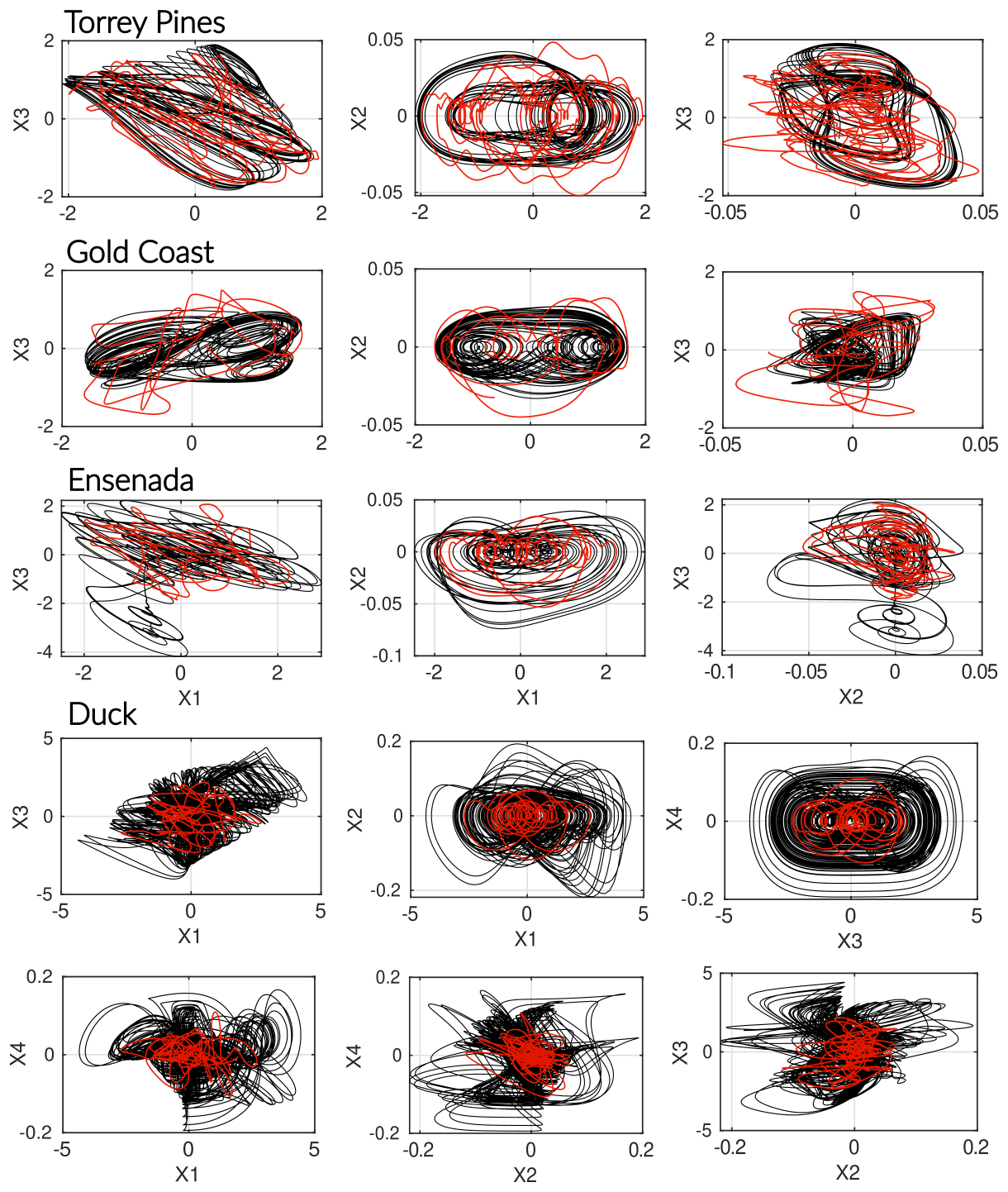
Figure 3 Comparison of observed (red) and modeled (black) phase spaces. For the three-dimensional models (Gold Coast, Torrey Pines, Ensenada), each portrait of the reconstructed attractor is shown. All systems exhibit a coherent shoreline–sandbar (X₁–X₃) coupling, with a clear negative linear relationship in Torrey Pines and Ensenada, whereas Gold Coast displays an inverted correlation pattern at seasonal scale. The four-dimensional model (Duck) reveals a markedly more intricate structure, characterized by strong nonlinear interactions among variables and the absence of any simple linear dependency between shoreline and sandbar positions (X₁–X₃). The inferred GPoM models successfully reproduce site-specific attractors and capture the essential geometry of the underlying morphodynamic phase space.

3 Results

3.1 Model–data comparison and spectral consistency

3.1.1 Phase space projections

The phase spaces derived from the GPoM autonomous models (see system equations in Sect. 3.2) are here compared to the dynamics directly reconstructed from the observed time series (Fig. 3). First, it should be noted that the modeled and observed trajectories are not expected to coincide pointwise in phase space. Indeed, the objective of the approach is to reproduce the original vector field, which is independent of the initial conditions. Even if the original phase space were perfectly modeled, any difference in the initial conditions would lead to a different trajectory. In the present case, the initial conditions are known with a finite level of precision, and the modeled phase space is a low-dimensional approximation of the original one, meaning that higher-dimensional (stochastic) perturbations are not represented in the model. Therefore, the comparison is not intended to assess trajectory-level agreement. Local mismatches are clearly visible in the phase portraits, particularly at small scales and during rapid excursions, reflecting differences in timing, unresolved variability, and the smoothing inherent to reduced-order reconstructions. The relevant comparison instead concerns the global organization of the phase space, including characteristic oscillatory loops, asymmetries, and state-dependent variability, without aiming at pointwise or trajectory-level agreement. With these elements in mind, the models are found to reproduce consistently the observed dynamics of shoreline–sandbar systems across all study sites, both in terms of amplitude and state-space density. The dominant geometric structures of the observed dynamics are largely recovered. Moreover, the models were integrated over extended periods (80 years) to assess their numerical stability and allow the full attractor to unfold in phase space. As a result, the system may occasionally visit states not sampled during the observational time window, yet remain dynamically consistent with the reconstructed equations. This property illustrates the model's ability to generalize beyond the training dataset while preserving its intrinsic dynamical organization.

To further assess the quality of the phase-space reconstruction, additional phase-space projections are provided in Appendix B. These projections (Figs. B5 and B6) confirm the overall geometric consistency between modeled and observed trajectories beyond what is visible in two-dimensional projections. Because it is difficult to go further in the comparison between the original and modeled phase space from a deterministic point of view, alternative spectral and statistical validation approaches may instead be considered (see next Sect. 3.1.2).

For the three-dimensional models (Gold Coast, Torrey Pines, Ensenada), each projection of the attractor reveals a coherent morphodynamic coupling between shoreline position (X₁), its temporal derivative (X₂), and sandbar position (X₃). At Torrey Pines and Ensenada (Eqs. 5 and 7), the system oscillates along a quasi-linear negative correlation between shoreline and sandbar positions (X₁–X₃) at seasonal timescales, consistent with a coupled retreat–recovery mechanism: when wave energy increases during winter, the sandbar migrates offshore while the shoreline retreats. This correlation suggests that the sandbar response is not fast enough to dissipate the enhanced wave energy, reducing its protective role and leading to greater shoreline retreat. During calmer periods, the sandbar slowly migrates landward, promoting shoreline recovery and closing the oscillatory cycle captured by the model. In contrast, the Gold Coast system (Eq. 6) displays an inverted correlation pattern, showing that the shoreline-sandbar system evolves as one, responding similarly to incoming forcing.

For the 3 models, the (X₂–X₁) portrait is the typical projection of a differential phase space involving an observable and its first-order derivative (Fig. 3). In such a representation, the shape of the trajectory reflects the underlying restoring and dissipative mechanisms of the system. The attractors observed here indicate a combination of 2 oscillatory processes in which shoreline position (X₁) oscillates around a single equilibrium point for Torrey Pines and Ensenada, under the restoring action of sandbar-mediated feedbacks and the cyclicity imposed by the annual cycle. For Gold Coast, the attractor evolves around 2 equilibrium points (located close to ($-\mathrm{1},\mathrm{0}$) and (1,0) in the (X₁,X₂) projection), and a third one situated between them (close to (0,0)), which enables alternation between the 2 equilibria or the emergence of larger loops connecting them. The amplitude of the loops provide insight into the system's stability and rate of energy exchange. Extended, large-amplitude loops indicate stronger seasonal variability and larger-scale shoreline adjustments, whereas numerous smaller, short-lived loops reflect disruptive short-term events (e.g., storms, intra-seasonal variability). The amplitude of these smaller loops further reveals the system's capacity to damp the morphological imprint of such disturbances, thus reflecting its resilience. At Torrey Pines, the observational data (red within Fig. 3) exhibit wide, extended loops involving 2 main branches, indicative of a highly energetic system dominated by strong seasonal variability and pronounced morphological exchanges. The numerous more rounded shorter loops suggest a superimposed contribution of storm-scale fluctuations. The model reproduces the overall extent of the attractor, capturing the main envelope of variability and the large-scale cyclic behavior, but with smoother trajectories, implying that part of the short-term perturbations and their damping–recovery dynamics are smoothed (i.e. high dimensional dynamics associated with noise has been filtered). The dynamical complexity observed at Torrey Pines ultimately converges to a period-two cycle, suggesting a metastable chaotic regime that may be triggered by temporary variations in the system (e.g. tides, mesoscale eddies, coastal storms). In contrast, at both Gold Coast and Ensenada, the model successfully reproduces the occurrence of both small and large loops, suggesting a more representative behavior across the system's spatiotemporal scales. The (X₃–X₂) projection highlights the joint variability between sandbar position and shoreline rate of change, reflecting the co-evolution of both components within the same morphodynamic feedback loop. The sandbar position (X₃) encapsulates the system's longer-term adjustment to hydrodynamic conditions, while the shoreline rate (X₂) expresses the more immediate response of the beach. The attractor geometry thus encompasses the phase relationship between these 2 timescales (making it the less evident projection to interpret only through observations). At Torrey Pines, Gold Coast and Ensenada, the trajectories form elongated, looping structures, indicating that sandbar migration and shoreline motion are phase-shifted, with delayed recovery of the shoreline once the sandbar returns landward. This reflects a coupled oscillatory system where energy is alternately stored in sandbar migration and released through shoreline adjustment. Therefore, these portraits reveal the mutual, rather than unidirectional, influence between the sandbar and shoreline components of the system for all 3 sites.

The four-dimensional model obtained at Duck exhibits a markedly more intricate phase-space organization, with multiple intertwined trajectories and a complex structure reflecting strong nonlinear coupling among the shoreline, sandbar, and their respective derivatives (X₂,X₄). In the (X₂–X₁) projection, broad nested loops and secondary sub-cycles indicate an oscillator governed by several interacting timescales, consistent with a system where rapid morphological responses are superimposed on slower morphodynamic adjustments. The (X₃–X₁) projection displays a folded, asymmetric attractor in which the trajectory slope reverses across the domain. This departure from the more linear correlation observed at other sites suggests that the coupling between shoreline and sandbar is not stationary but alternates between regimes of weak and strong interaction. In the (X₃–X₂) plane, spiral-like loops around the origin denote delayed responses between sandbar position and shoreline velocity as the shoreline adjusts to sandbar migration with a phase lag. The amplitude variability within these spirals reflects intermittent shifts in coupling strength, possibly associated with episodic energetic events or memory effects in sediment redistribution. The (X₄–X₁) projection, linking shoreline position to sandbar migration rate, reveals a pronounced asymmetry: rapid offshore sandbar motion (X₄<0) corresponds to abrupt shoreline retreat, whereas onshore sandbar migration (X₄>0) is associated with a slower and more gradual recovery. This hysteresis indicates that the system retains a morphodynamic memory of past energetic states and/or that the threshold required to trigger significant morphological change depends on whether energy is increasing or decreasing. The (X₄–X₂) projection reveals a nonlinear relationship, showing that shoreline and sandbar velocities are not independent. Their interaction varies with the system state, suggesting a potentially intermittent coupling. The (X₃–X₄) projection isolates the intrinsic sandbar dynamics, showing concentric, nested cycles that are typical of systems organized around 2 main pseudo-periods. The observed dynamics are not quasi-periodic but may derive from such behavior, suggesting toroidal chaos.

The high complexity of the Duck model derived using GPoM is consistent with field observations of sandbar dynamics, where the inherited fall morphology exerts a strong control on the subsequent year's morphological evolution (Anderson et al., 2023). This behavior reflects a pronounced sensitivity to initial conditions, as the pre-existing sandbar configuration constrains the system's response to comparable hydrodynamic forcing, leading to path-dependent and potentially hysteresis dynamics. Moreover, Duck belongs to a beach type characterized by an active sandbar that slowly migrates offshore with aperiodic consistency, before being replaced by a newly active bar forming at the breaker line; a behavior commonly referred to as Net Offshore Migration (NOM) (Ruessink et al., 2009). In this study, only the active sandbar is considered, and therefore this phenomenon does not explicitly appear within our dataset. Nevertheless, this additional level of complexity may not be uncorrelated with the complex attractor geometry and higher-order nonlinear terms revealed by the model as the NOM behavior is known to be strongly conditioned by the antecedent beach state (Plant et al., 1999; Ruessink et al., 2003), which could reflect the memory and cumulative effects inherent to these episodic-to-interannual bar exchanges.

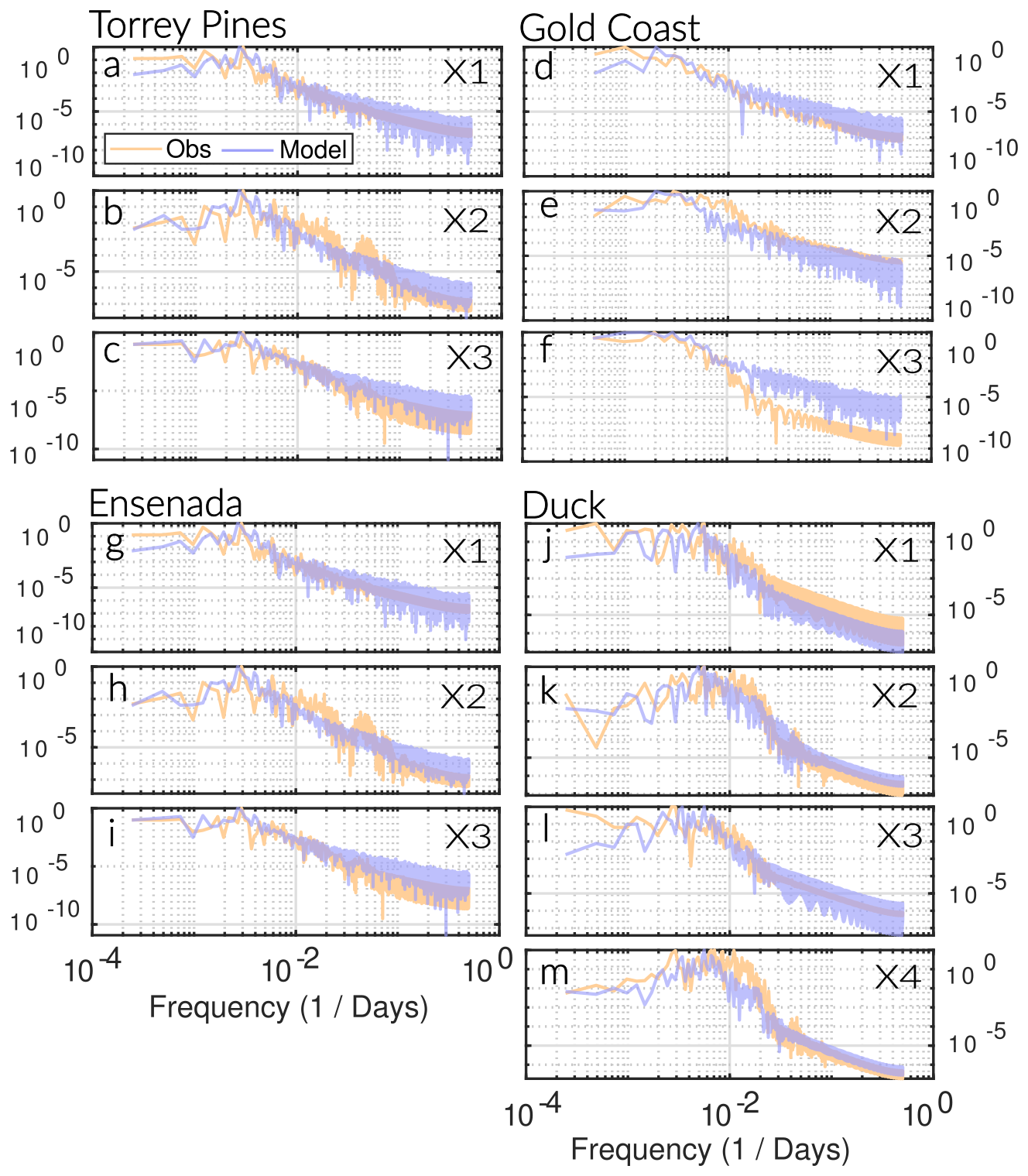
Figure 4 Comparison of normalized spectral power density between observations and models. Each variable's spectrum obtained from the model (light purple) is plotted against its corresponding observation (light orange). The modeled energy distribution closely matches that of the observed data, indicating that the models successfully reproduce the dynamical variability of the systems they were inferred from. At low frequencies (10⁻⁴–10⁻³ d⁻¹), the slow components of the shoreline–sandbar system are well captured, reflecting a realistic long-term memory and morphodynamic coupling. The model also reproduces the seasonal to monthly dynamics (around 10⁻² d⁻¹) with good accuracy. At higher frequencies (> 10⁻² d⁻¹), the energetic slope remains consistent between model and observations, without overestimation of short-term variability, suggesting that the GPoM-based dynamics naturally filter the high-frequency noise while preserving the dominant physical scales of variability. The broadband power-law spectra ($P\left(f\right)\sim f^{-\mathit{\alpha }}$) indicate that the shoreline–sandbar system exhibits long-term memory and self-organized, chaotic dynamics, with energy cascading smoothly from low-frequency morphodynamic cycles to higher-frequency storm-driven responses.

3.1.2 Models spectral and statistical consistency

The spectral analysis provides a detailed verification of the temporal consistency between observed and modeled dynamics (Fig. 4). For each site, the normalized power spectra of the modeled variables (light purple) closely reproduce those derived from the observations (light orange) over several orders of magnitude in frequency. At low frequencies (10⁻⁴–10⁻³ d⁻¹), the models capture the slow morphodynamic components associated with long-term shoreline–sandbar co-variability, reflecting the system's memory and adjustment at interannual timescales. At intermediate frequencies (10⁻³–10⁻² d⁻¹), both observed and modeled spectra exhibit distinct shoulders or inflection points, corresponding to the annual to intra-seasonal response of the system to modulations in wave energy. This indicates that the inferred equations successfully embed the transfer mechanisms linking external forcing to shoreline–sandbar exchanges. At higher frequencies (> 10⁻² d⁻¹), the energetic slope remains consistent between models and observations, without evidence of artificial energy accumulation or damping. The realistic high-frequency decay of the model spectra indicates that the deterministic GPoM formulations reproduce an effective loss of dynamical memory at short timescales, preventing the accumulation of spurious small-scale variability and ensuring that trajectories remain bounded and confined to a finite attractor, even in the absence of explicit stochastic forcing.

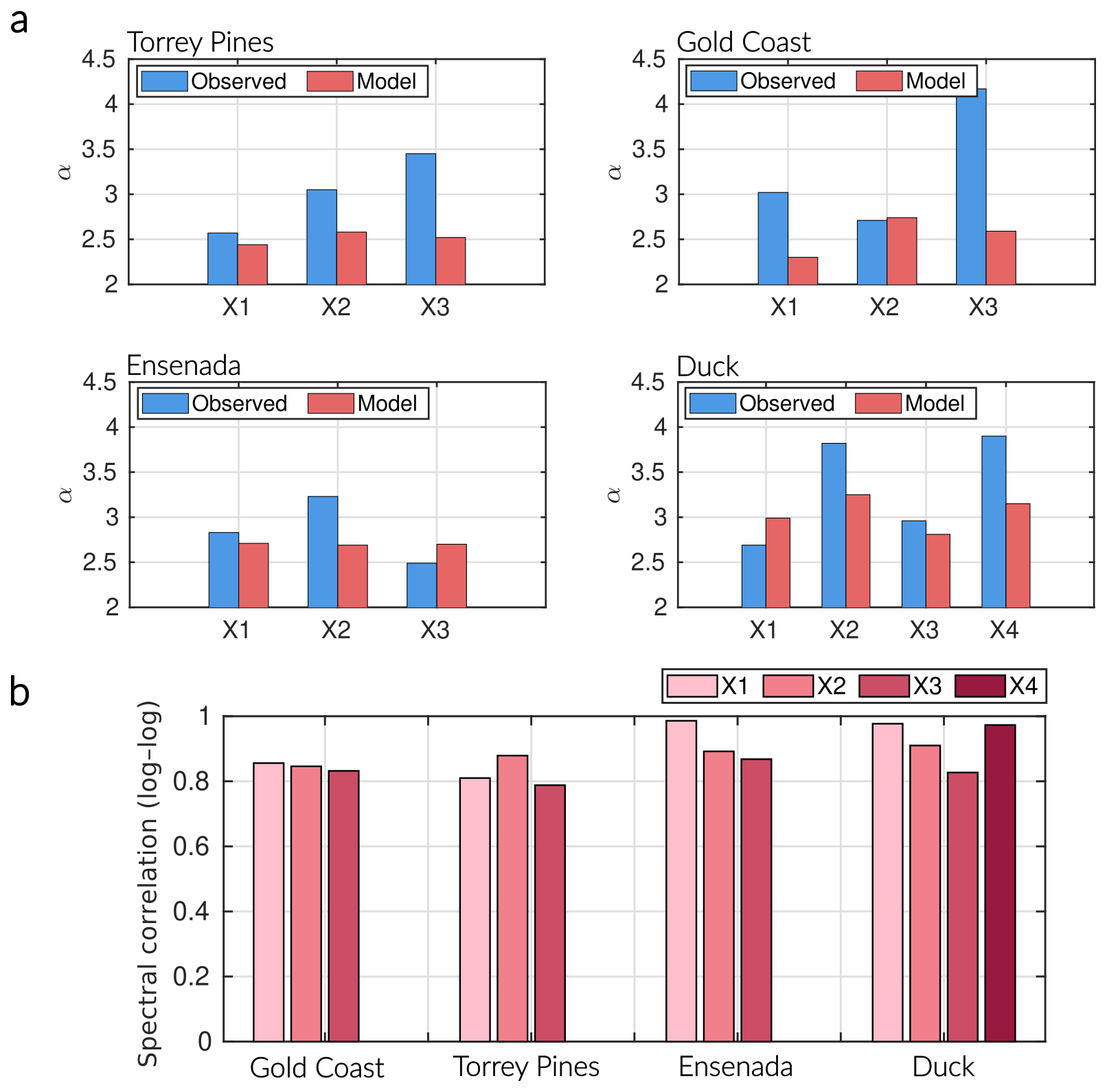
Figure 5 Spectral comparison between observed and modeled dynamics. (a) Comparison of spectral slopes (α) for each variable and site. Both observations (blue) and GPoM models (red) exhibit red-to-brown noise behavior (α≈ 2.5–4), indicating scale-invariant, long-memory morphodynamic variability. (b) Spectral correlations (log–log) between observed and modeled spectra show consistently high values (r > 0.8), confirming that the inferred nonlinear dynamics reproduce the observed energy distribution across temporal scales. The GPoM models capture both the scaling and spectral energy structure of the shoreline–sandbar systems, reflecting a realistic transfer of energy from low-frequency morphodynamic oscillations to higher-frequency storm-driven variability.

To quantitatively assess model–data fidelity, the comparison of spectral slopes and correlations provides a complementary approach to ensure for the models' dynamical consistency (Fig. 5). Across all sites, the spectral exponents derived from the models remain consistent with those obtained from the observations, confirming that both share similar scaling laws and temporal persistence (α≈ 2.5–4). Spectral correlations exceeding r>0.8 in most cases indicate that the models reproduce not only the dominant frequencies but also the overall energy distribution across temporal scales. Slightly flatter spectral slopes in the modeled series likely reflect the smoothing effect inherent to deterministic low-dimensional reconstructions, which capture organized dynamics but not high-frequency stochastic variability (Mangiarotti et al., 2012, 2016). Nevertheless, the agreement across frequencies spanning more than 3 decades supports the conclusion that the GPoM-derived equations capture the multiscale organization and memory-driven nature of real shoreline–sandbar dynamics. It is important to note that these models are entirely autonomous: no external forcing has been prescribed, and the variability observed in their dynamics arises solely from the intrinsic couplings reconstructed from the data. The influence of external drivers such as wave climate or sea level modulations is thus implicitly embedded in the model structure itself.

These results show that the GPoM models satisfactorily reconstruct the essential physics of the sites observables directly from observational data. They capture the nonlinear coupling between shoreline and sandbar, the characteristic oscillatory attractors, and the broadband red spectral behavior; typical from natural coastal systems (Ruessink et al., 2007; Pianca et al., 2015). As such, the models can be viewed as compact, deterministic reduced-order representations of the observed dynamics, capable of reproducing their key statistical and structural properties, and suitable for further investigation of the system's intrinsic dynamics and shoreline–sandbar coupling. Of course, spectral consistency alone does not uniquely constrain the underlying dynamical structure as distinct dynamical systems can share similar power-law spectra while differing fundamentally in their phase-space geometry. The spectral validation presented here is therefore a necessary but not sufficient condition for the validity assessment of the reconstructed dynamics. To complement this, the forecasting error growth was also estimated for each model, providing a statistical view of model performance. The horizon of predictability HP_{25 %,90 %} varies from 0.5 to 1 month, depending both on the model and on the instability of the dynamics (see Sect. 3.3). Unfortunately, there are no equivalent autonomous models against which these performances can be easily compared. Nevertheless, one can refer to analyses based on neural networks, which clearly show that error growth sharply increases during the first 50 to 100 d (Pape et al., 2007). It can also be noted that characteristic times ranging from 15 to 30 d are commonly used to simulate cross-shore evolution, and much shorter timescales of 0.5 to 6 d during very rapid events (Hewageegana and Canestrelli, 2021); these characteristic prediction times, over which satisfactory predictions are obtained, are consistent with the predictability of the GPoM models. Finally, a histogram of the distributions of the variables (Figs. B1–B4) and the associated statistical moments from first to fourth order (Table B1) show that the models consistently reproduce the statistical properties of most state variables, including the shape, spread, and asymmetry of their distributions across all sites. As with spectral properties, the variable distributions do not uniquely characterize the underlying dynamical structure. Hence, the validation presented here is therefore a necessary, but not sufficient, condition for model assessment.

3.2 Reconstructed equations, model structures and physical interpretation of dominant terms

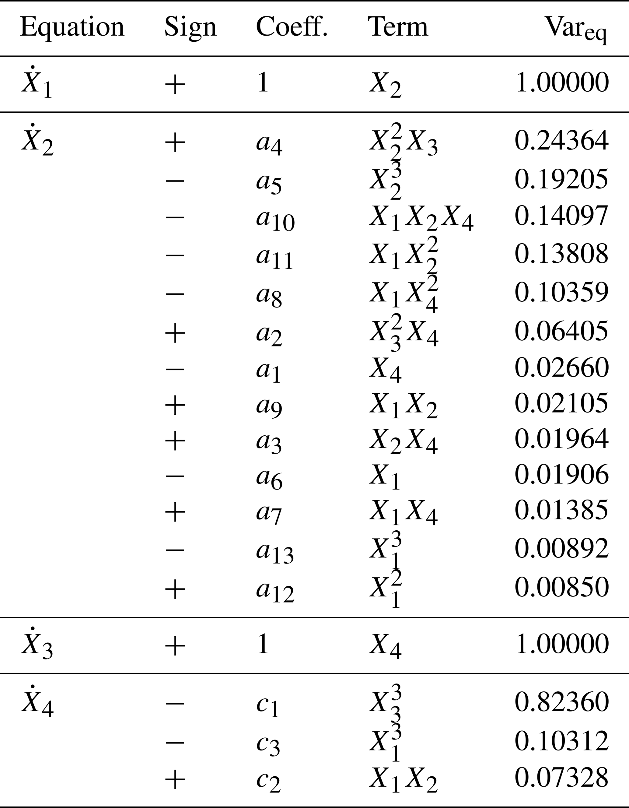
The autonomous polynomial models reconstructed for each site are presented in Eqs. (6)–(8). All systems follow a canonical form in which the first equation expresses the temporal derivative of the shoreline position (${\dot{X}}_{\mathrm{1}}=X_{\mathrm{2}}$), while the subsequent equations describe the nonlinear coupling between shoreline acceleration (${\dot{X}}_{\mathrm{2}}$) and sandbar dynamics (X₃, and X₄ for Duck).

$$\begin{array}{}\text{(5)}& \text{Torrey\hspace{0.17em}\hspace{0.17em}Pines}\left\{\begin{array}{ll}{\dot{X}}_{\mathrm{1}}=& X_{\mathrm{2}},\\ {\dot{X}}_{\mathrm{2}}=& a_{\mathrm{1}}{X}_{\mathrm{3}}+a_{\mathrm{2}}{X}_{\mathrm{3}}^{\mathrm{3}}+a_{\mathrm{3}}{X}_{\mathrm{2}}{X}_{\mathrm{3}}^{\mathrm{2}}\\ & +a_{\mathrm{4}}{X}_{\mathrm{2}}^{\mathrm{2}}{X}_{\mathrm{3}}+a_{\mathrm{5}}{X}_{\mathrm{1}}{X}_{\mathrm{3}}^{\mathrm{2}}\\ & +a_{\mathrm{6}}{X}_{\mathrm{1}}^{\mathrm{2}}{X}_{\mathrm{3}}+a_{\mathrm{7}}{X}_{\mathrm{1}}^{\mathrm{3}},\\ {\dot{X}}_{\mathrm{3}}=& b_{\mathrm{1}}+b_{\mathrm{2}}{X}_{\mathrm{3}}+b_{\mathrm{3}}{X}_{\mathrm{2}}+b_{\mathrm{4}}{X}_{\mathrm{3}}^{\mathrm{3}}\\ & +b_{\mathrm{5}}{X}_{\mathrm{2}}{X}_{\mathrm{3}}^{\mathrm{2}}+b_{\mathrm{6}}{X}_{\mathrm{2}}^{\mathrm{2}}+b_{\mathrm{7}}{X}_{\mathrm{2}}^{\mathrm{2}}{X}_{\mathrm{3}}\\ & +b_{\mathrm{8}}{X}_{\mathrm{1}}+b_{\mathrm{9}}{X}_{\mathrm{1}}{X}_{\mathrm{2}}{X}_{\mathrm{3}}\\ & +b_{\mathrm{10}}{X}_{\mathrm{1}}{X}_{\mathrm{2}}^{\mathrm{2}}+b_{\mathrm{11}}{X}_{\mathrm{1}}^{\mathrm{2}}{X}_{\mathrm{2}}.\end{array}\right.\end{array}$$

$$\begin{array}{}\text{(6)}& \text{Gold\hspace{0.17em}\hspace{0.17em}Coast}\left\{\begin{array}{ll}{\dot{X}}_{\mathrm{1}}& =X_{\mathrm{2}},\\ {\dot{X}}_{\mathrm{2}}& =a_{\mathrm{1}}{X}_{\mathrm{3}}+a_{\mathrm{2}}{X}_{\mathrm{3}}^{\mathrm{3}}+a_{\mathrm{3}}{X}_{\mathrm{2}}{X}_{\mathrm{3}}\\ & +a_{\mathrm{4}}{X}_{\mathrm{2}}^{\mathrm{2}}{X}_{\mathrm{3}}+a_{\mathrm{5}}{X}_{\mathrm{1}}+a_{\mathrm{6}}{X}_{\mathrm{1}}{X}_{\mathrm{3}}^{\mathrm{2}}\\ & +a_{\mathrm{7}}{X}_{\mathrm{1}}{X}_{\mathrm{2}}^{\mathrm{2}}+a_{\mathrm{8}}{X}_{\mathrm{1}}^{\mathrm{2}}{X}_{\mathrm{3}}+a_{\mathrm{9}}{X}_{\mathrm{1}}^{\mathrm{3}},\\ {\dot{X}}_{\mathrm{3}}& =b_{\mathrm{1}}+b_{\mathrm{2}}{X}_{\mathrm{3}}+b_{\mathrm{3}}{X}_{\mathrm{2}}+b_{\mathrm{4}}{X}_{\mathrm{2}}{X}_{\mathrm{3}}^{\mathrm{2}}\\ & +b_{\mathrm{5}}{X}_{\mathrm{1}}^{\mathrm{2}}.\end{array}\right.\end{array}$$

$$\begin{array}{}\text{(7)}& {\displaystyle }\text{Ensenada:}\left\{\begin{array}{ll}{\dot{X}}_{\mathrm{1}}& =X_{\mathrm{2}},\\ {\dot{X}}_{\mathrm{2}}& =a_{\mathrm{1}}{X}_{\mathrm{3}}+a_{\mathrm{2}}{X}_{\mathrm{1}}{X}_{\mathrm{3}}^{\mathrm{2}}+a_{\mathrm{3}}{X}_{\mathrm{2}}\\ & +a_{\mathrm{4}}{X}_{\mathrm{1}}{X}_{\mathrm{2}}+a_{\mathrm{5}}{X}_{\mathrm{1}}{X}_{\mathrm{2}}{X}_{\mathrm{3}}+a_{\mathrm{6}}{X}_{\mathrm{1}}^{\mathrm{2}}{X}_{\mathrm{3}}\\ & +a_{\mathrm{7}}{X}_{\mathrm{1}}^{\mathrm{2}}{X}_{\mathrm{2}}+a_{\mathrm{8}}{X}_{\mathrm{1}}^{\mathrm{3}},\\ {\dot{X}}_{\mathrm{3}}& =b_{\mathrm{1}}+b_{\mathrm{2}}{X}_{\mathrm{3}}+b_{\mathrm{3}}{X}_{\mathrm{2}}+b_{\mathrm{4}}{X}_{\mathrm{2}}^{\mathrm{3}}\\ & +b_{\mathrm{5}}{X}_{\mathrm{1}}{X}_{\mathrm{3}}^{\mathrm{2}}+b_{\mathrm{6}}{X}_{\mathrm{1}}^{\mathrm{2}}{X}_{\mathrm{3}}+b_{\mathrm{7}}{X}_{\mathrm{1}}^{\mathrm{3}}\end{array}\right.\text{(8)}& {\displaystyle }\text{Duck:}\left\{\begin{array}{ll}{\dot{X}}_{\mathrm{1}}& =X_{\mathrm{2}},\\ {\dot{X}}_{\mathrm{2}}& =a_{\mathrm{1}}{X}_{\mathrm{4}}+a_{\mathrm{2}}{X}_{\mathrm{3}}^{\mathrm{2}}{X}_{\mathrm{4}}+a_{\mathrm{3}}{X}_{\mathrm{2}}{X}_{\mathrm{4}}\\ & +a_{\mathrm{4}}{X}_{\mathrm{2}}^{\mathrm{2}}{X}_{\mathrm{3}}+a_{\mathrm{5}}{X}_{\mathrm{2}}^{\mathrm{3}}+a_{\mathrm{6}}{X}_{\mathrm{1}}+a_{\mathrm{7}}{X}_{\mathrm{1}}{X}_{\mathrm{4}}\\ & +a_{\mathrm{8}}{X}_{\mathrm{1}}{X}_{\mathrm{4}}^{\mathrm{2}}\\ & +a_{\mathrm{9}}{X}_{\mathrm{1}}{X}_{\mathrm{2}}+a_{\mathrm{10}}{X}_{\mathrm{1}}{X}_{\mathrm{2}}{X}_{\mathrm{4}}+a_{\mathrm{11}}{X}_{\mathrm{1}}{X}_{\mathrm{2}}^{\mathrm{2}}\\ & +a_{\mathrm{12}}{X}_{\mathrm{1}}^{\mathrm{2}}+a_{\mathrm{13}}{X}_{\mathrm{1}}^{\mathrm{3}},\\ {\dot{X}}_{\mathrm{3}}& =X_{\mathrm{4}},\\ {\dot{X}}_{\mathrm{4}}& =c_{\mathrm{1}}{X}_{\mathrm{3}}^{\mathrm{3}}+c_{\mathrm{2}}{X}_{\mathrm{1}}{X}_{\mathrm{2}}+c_{\mathrm{3}}{X}_{\mathrm{1}}^{\mathrm{3}}.\end{array}\right.\end{array}$$

Table 1 Models' coefficient weights comparison for the 4 sites of study.

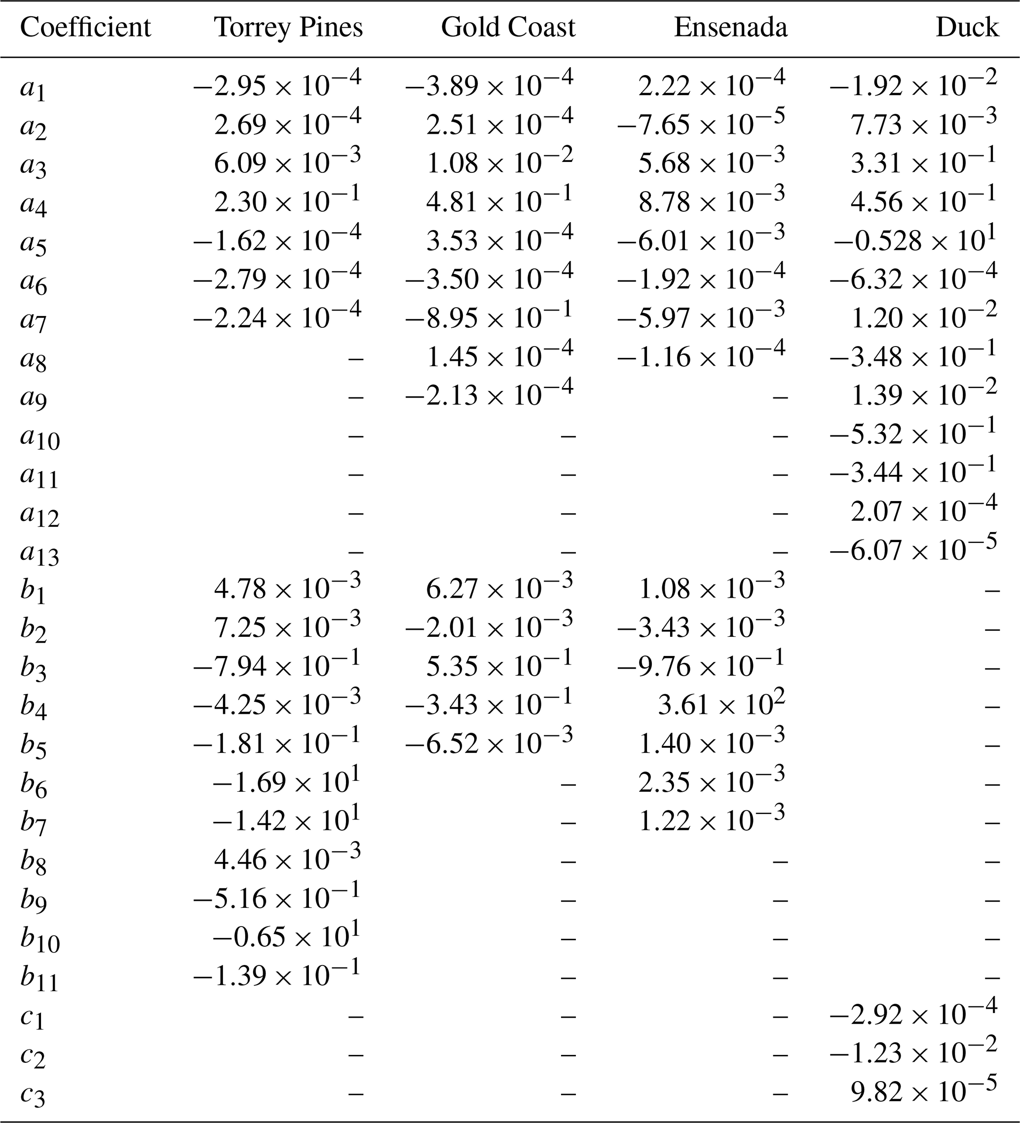
The reconstructed equations are third-order polynomial systems, containing respectively 19, 15, 16, and 18 K terms for Torrey Pines, Gold Coast, Ensenada, and Duck. Each model combines quadratic and cubic cross-interactions together with self-interacting terms. In these models, feedbacks between shoreline position, sandbar position, and their respective temporal derivatives jointly govern the observed variability. Although several of their respective terms exhibit relatively small amplitudes (Table 1), they contribute critically to the global stability of the reconstructed attractor by shaping its fine-scale curvature and preventing divergence during long integrations. This behavior is consistent with the GPoM algorithm design, which prioritizes preservation of the phase-space geometry over direct time-series correlation between data and model (Mangiarotti et al., 2012). As such, the equations obtained are an approximate and reduced formulation of the original ones. Hence, several physical processes may have been compressed into a single shared monomial, which limits the mechanical interpretation, since each term can no longer be viewed as an independent process. Likewise, complementary contributions may not appear in the equations derived by GPoM, which makes it more difficult to clearly distinguish the physical processes underlying the system dynamics.

Consequently, the interpretation should focus on the dominant terms (those with the largest variance within their respective equations) while acknowledging that weaker nonlinearities collectively ensure attractor coherence and long-term stability. Here, for each model, we provide a rewritten form of the equation from a mechanistic viewpoint in terms of the forces F_i applied to the sand masses (Eqs. A4–12), positions X_i and speed V_i, and using only the terms with a variance of Var_eq≥ 10 % (Tables 2– 5), accompanied by fluence diagrams (Mason, 1953) to support the physical interpretation (Fig. 6). V₁ and V₃ notation are fostered instead of X₂ and X₄ to facilitate the interpretation. The details of these rewritten forms are given in the appendix (see Appendix A).

$$\begin{array}{}\text{(9)}& \text{Torrey\hspace{0.17em}\hspace{0.17em}Pines}\left\{\begin{array}{ll}{\mathit{F}}_{\mathrm{1}}& =-a_{\mathrm{7}}{X}_{\mathrm{1}}^{\mathrm{2}}{\mathit{X}}_{\mathrm{1}}+a_{\mathrm{2}}{X}_{\mathrm{3}}^{\mathrm{2}}{\mathit{X}}_{\mathrm{3}}\\ & -a_{\mathrm{6}}{X}_{\mathrm{1}}^{\mathrm{2}}{\mathit{X}}_{\mathrm{3}},\\ {\mathit{F}}_{\mathrm{3}}& =-b_{\mathrm{3}}{\mathit{F}}_{\mathrm{1}}-\mathrm{3}{b}_{\mathrm{4}}{X}_{\mathrm{3}}^{\mathrm{2}}{\mathit{V}}_{\mathrm{3}}\end{array}\right.\end{array}$$

$$\begin{array}{}\text{(10)}& {\displaystyle }\text{Gold\hspace{0.17em}\hspace{0.17em}Coast}\left\{\begin{array}{ll}{\mathit{F}}_{\mathrm{1}}& =-a_{\mathrm{9}}{X}_{\mathrm{1}}^{\mathrm{2}}{\mathit{X}}_{\mathrm{1}}+a_{\mathrm{5}}{\mathit{X}}_{\mathrm{1}}-a_{\mathrm{1}}{\mathit{X}}_{\mathrm{3}},\\ {\mathit{F}}_{\mathrm{3}}& =b_{\mathrm{3}}{\mathit{F}}_{\mathrm{1}}-\mathrm{2}{b}_{\mathrm{5}}{X}_{\mathrm{1}}{\mathit{V}}_{\mathrm{1}}\end{array}\right.\text{(11)}& {\displaystyle }\text{Ensenada:}\left\{\begin{array}{ll}{\mathit{F}}_{\mathrm{1}}& =-a_{\mathrm{8}}{X}_{\mathrm{1}}^{\mathrm{2}}{\mathit{X}}_{\mathrm{1}}-a_{\mathrm{6}}{X}_{\mathrm{1}}^{\mathrm{2}}{\mathit{X}}_{\mathrm{3}}+a_{\mathrm{1}}{\mathit{X}}_{\mathrm{3}},\\ {\mathit{F}}_{\mathrm{3}}& =-b_{\mathrm{3}}{\mathit{F}}_{\mathrm{1}}+\mathrm{3}{b}_{\mathrm{4}}{X}_{\mathrm{2}}^{\mathrm{2}}{\mathit{F}}_{\mathrm{1}}\end{array}\right.\text{(12)}& {\displaystyle }\text{Duck:}\left\{\begin{array}{ll}{\mathit{F}}_{\mathrm{1}}& =a_{\mathrm{4}}{V}_{\mathrm{1}}^{\mathrm{2}}{\mathit{X}}_{\mathrm{3}}-a_{\mathrm{5}}{V}_{\mathrm{1}}^{\mathrm{2}}{\mathit{V}}_{\mathbf{1}}-a_{\mathrm{10}}{V}_{\mathrm{1}}{V}_{\mathrm{3}}{\mathit{X}}_{\mathrm{1}}\\ & -a_{\mathrm{11}}{V}_{\mathrm{1}}^{\mathrm{2}}{\mathit{X}}_{\mathrm{1}}-a_{\mathrm{8}}{V}_{\mathrm{3}}^{\mathrm{2}}{\mathit{X}}_{\mathrm{1}},\\ {\mathit{F}}_{\mathrm{3}}& =c_{\mathrm{1}}{X}_{\mathrm{3}}^{\mathrm{2}}{\mathit{X}}_{\mathrm{3}}+c_{\mathrm{3}}{X}_{\mathrm{1}}^{\mathrm{2}}{\mathit{X}}_{\mathrm{1}}\end{array}\right.\end{array}$$

Table 2 Analysis of variance of the GPoM model – site of Torrey Pines. The variances are normalized by equation (Var_eq) and at the scale of the entire model (Var_global).

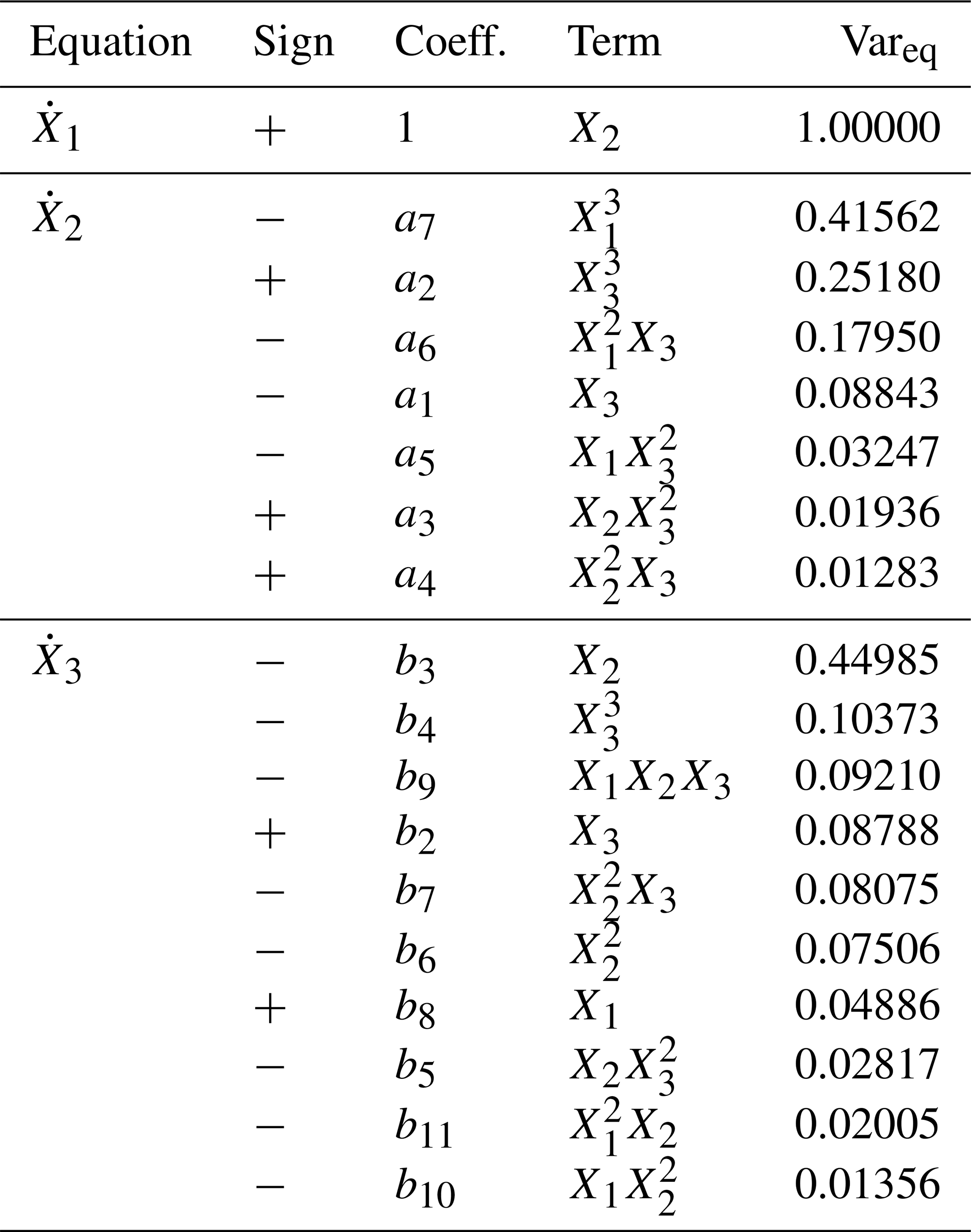
Table 3 Analysis of variance of the GPoM model – site of Gold Coast. The variances are normalized by equation (Var_eq) and at the scale of the entire model (Var_global).

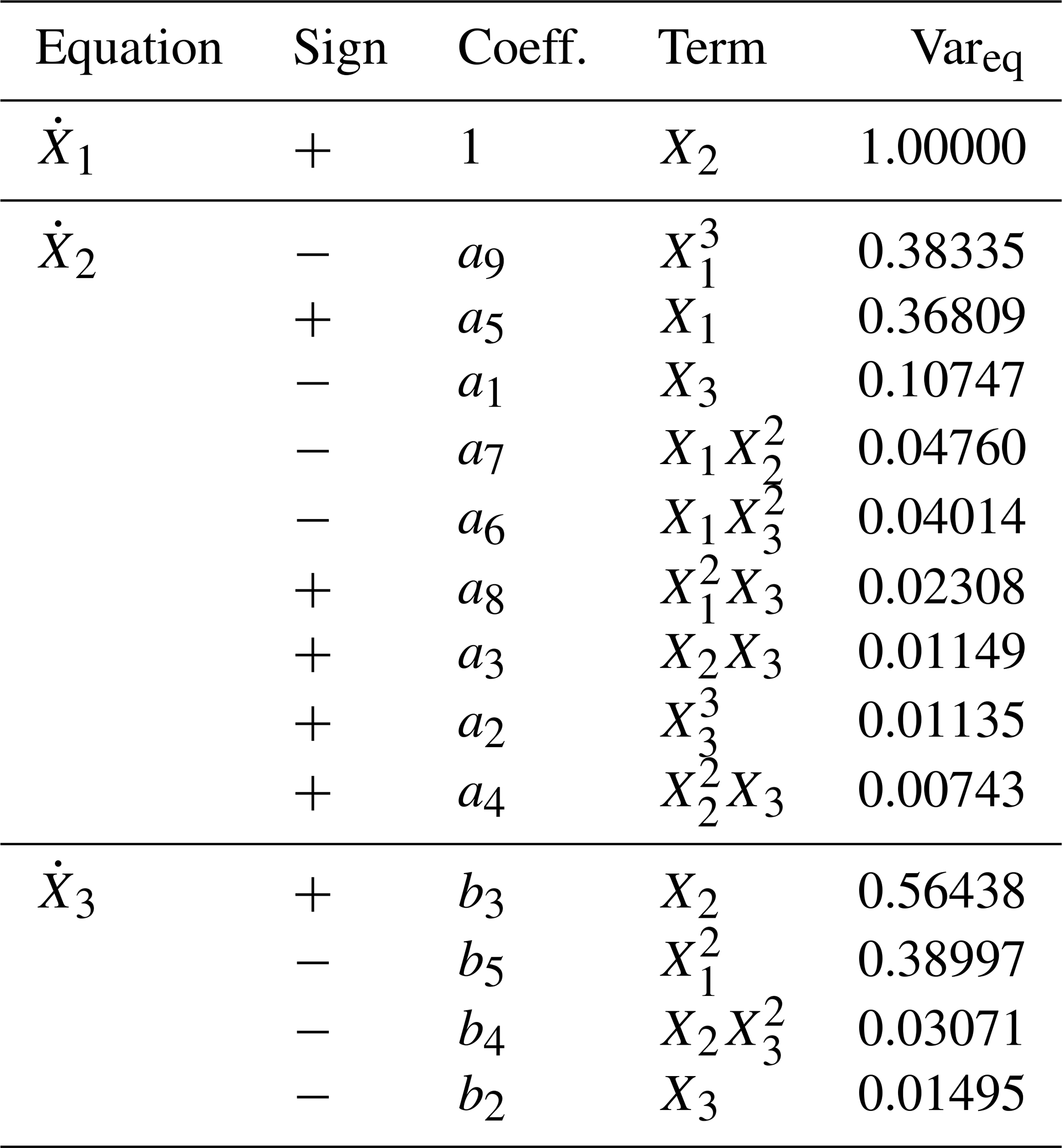
Table 4 Analysis of variance of the GPoM model – site of Ensenada. The variances are normalized by equation (Var_eq) and at the scale of the entire model (Var_global).

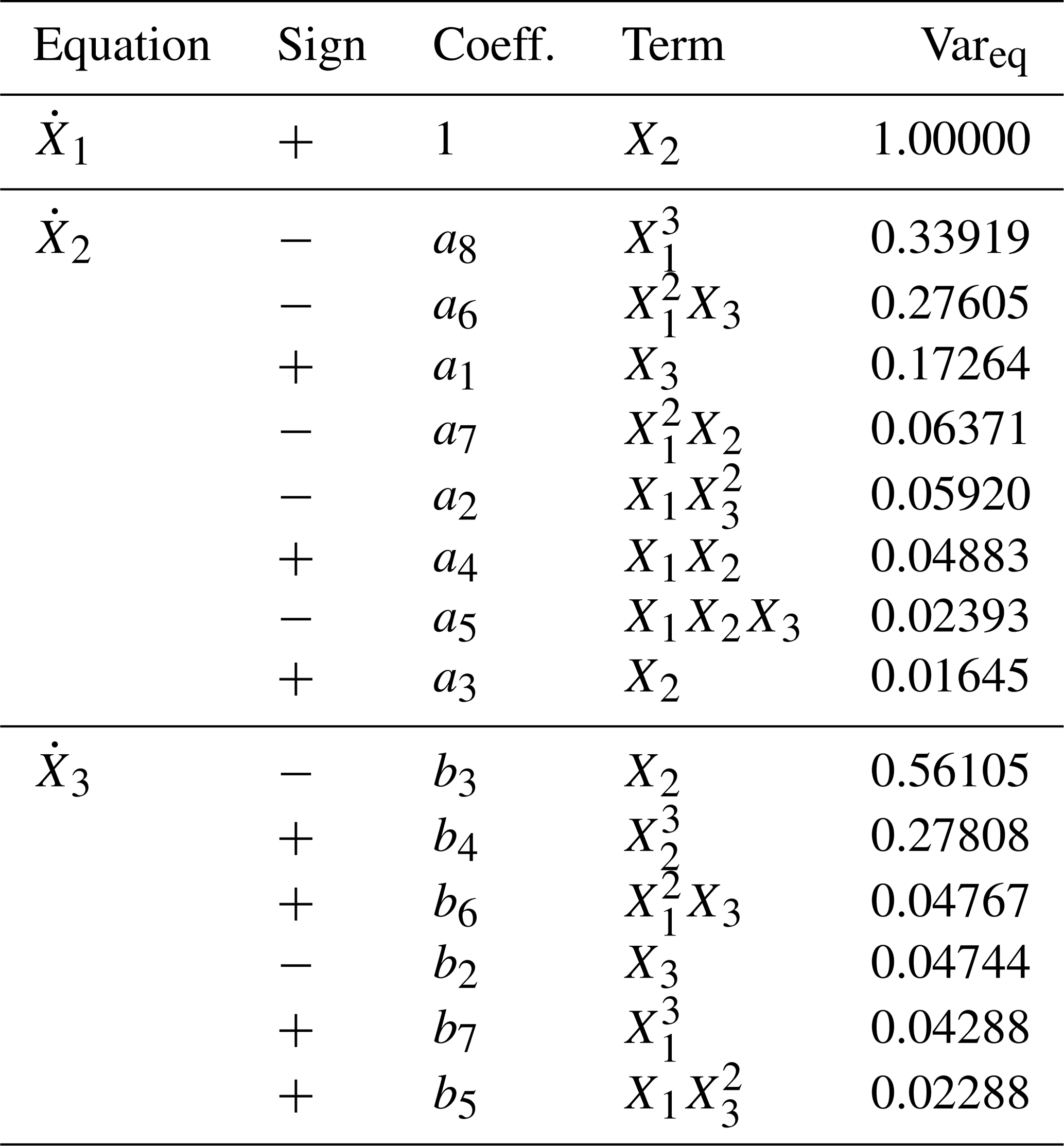
Table 5 Analysis of variance of the GPoM model – site of Duck. The variances are normalized by equation (Var_eq) and at the scale of the entire model (Var_global).

3.2.1 Torrey Pines

The variance-significant terms contributing to the shoreline dynamics (first equation in Eq. A4) highlight both the natural oscillatory behavior of the shoreline and the feedback exerted by the sandbar on its adjustment. The term $-a_{\mathrm{7}}{X}_{\mathrm{1}}^{\mathrm{2}}{\mathit{X}}_{\mathrm{1}}$ acts as a nonlinear restoring force that drives the shoreline position back toward the imposed equilibrium (X₁=0). Its cubic dependence implies a very weak response near equilibrium and a rapidly increasing restoring tendency for large excursions, consistent with the oscillatory behavior typically observed on wave-dominated sandy shorelines in the absence of other major external forcings (Dean, 1991; Yates et al., 2009). In contrast, the term $+a_{\mathrm{2}}{X}_{\mathrm{3}}^{\mathrm{2}}{\mathit{X}}_{\mathrm{3}}$ introduces a nonlinear destabilizing contribution transmitted from the sandbar dynamics to the shoreline. Because it scales with $X_{\mathrm{3}}^{\mathrm{3}}$, it strengthens the shoreline response when the sandbar undergoes large displacements. Generally speaking, the sandbar acts as an energy buffer when located close to the shoreline, reducing the effective wave energy forcing reaching the shore, whereas large offshore excursions reduce this buffering capacity and allow stronger forcing to be transmitted to the shoreline. As a result, far-from-equilibrium sandbar positions feed back onto the shoreline as an increasingly strong driving force, pushing its motion away from equilibrium. Finally, the term $-a_{\mathrm{6}}{X}_{\mathrm{1}}^{\mathrm{2}}{\mathit{X}}_{\mathrm{3}}$ represents a nonlinear cross–coupling between the shoreline position and the sandbar. Because $X_{\mathrm{1}}^{\mathrm{2}}$ modulates its magnitude, this contribution becomes significant only when the shoreline is strongly displaced. Its sign is controlled by X₃: sandbar excursions generate a forcing on the shoreline that opposes the sign of X₃, thereby acting as a nonlinear corrective influence transmitted from the sandbar to the shoreline.

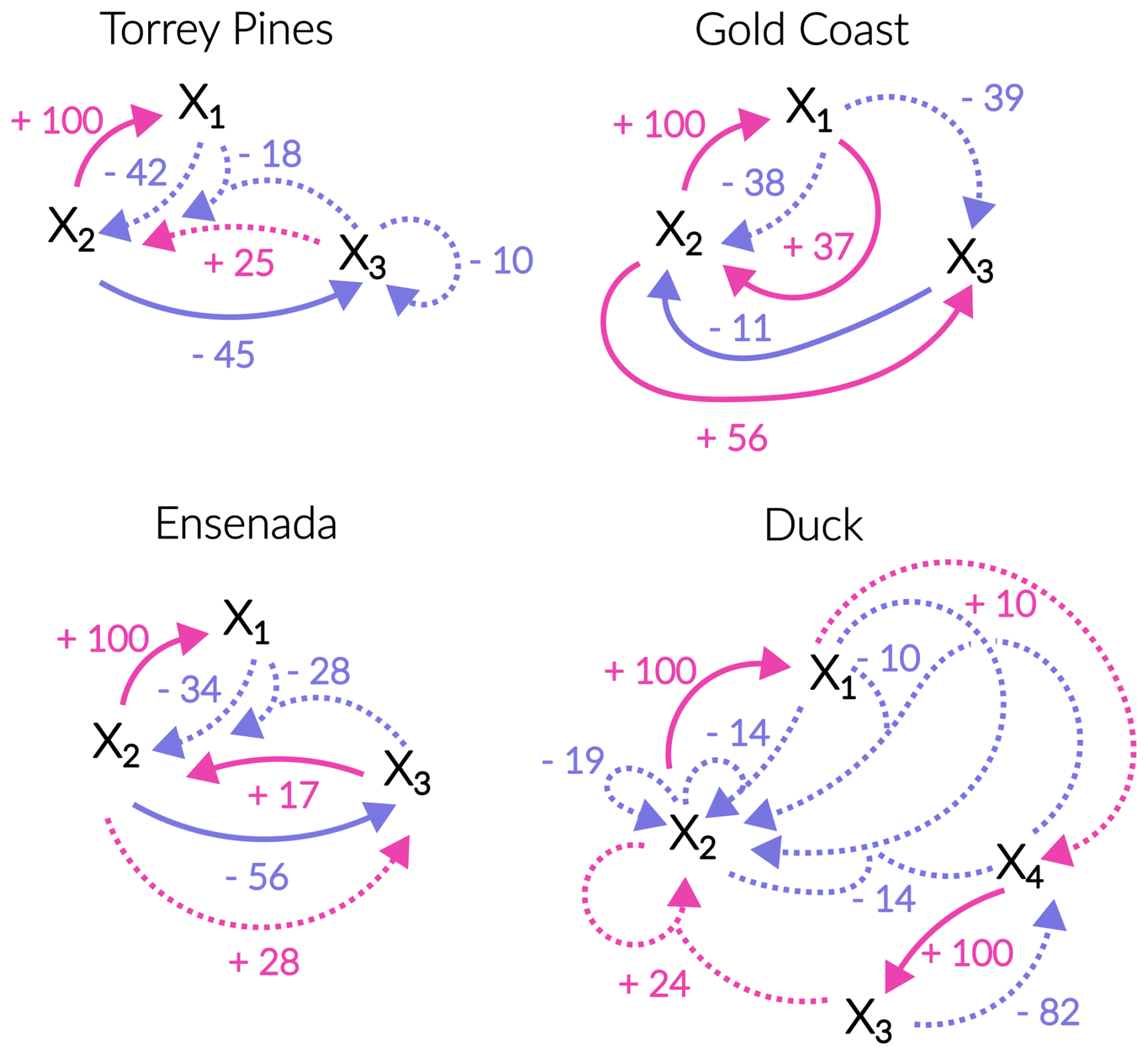
Figure 6 Fluence diagrams between the variables for the 4 sites. Fluence diagrams are presented to map the underlying positive (pink) and negative (light blue) feedback loops between variables, whether linear (solid lines) or nonlinear (dashed lines). The strength and sign of the feedback influence is derived directly from the variance explained by each term within its equation (Tables 2–5) and the sign of the associated coefficient (Table 1), respectively. Only terms accounting for 10 % or more of the signal variability are considered. Note that to account for the combined action of several variables, arrows with 2 inputs and a single output are used.

The equation governing the sandbar dynamics involves 2 variance-significant terms (second equation in Eq. A4). The first one, −b₂F₁, represents an anticorrelated coupling whereby the bar responds in the opposite direction to the forcing applied to the shoreline. Altogether with $-a_{\mathrm{6}}{X}_{\mathrm{1}}^{\mathrm{2}}{\mathit{X}}_{\mathrm{3}}$, this term captures the seasonal coupling within the shoreline–sandbar system: during winter, offshore sandbar migration accompanies shoreline retreat, while during summer, onshore bar migration accompanies shoreline advance. This behavior reflects an adaptive surf-zone system whose effective wave energy dissipation length adjusts to the seasonal modulation of incoming wave forcing, thereby enhancing system resilience between seasonal returns via dynamic feedback. This dynamical interpretation is supported by field observations at Torrey Pines, where the surf-zone width is well preserved between equivalent seasonal states each year (Aubrey et al., 1980; Winant et al., 1975). The second term, $-\mathrm{3}{b}_{\mathrm{4}}{X}_{\mathrm{3}}^{\mathrm{2}}{V}_{\mathrm{3}}$, acts as a nonlinear attenuation of the bar motion. Because the damping scales with $X_{\mathrm{3}}^{\mathrm{2}}$, the migration of the sandbar is only weakly damped near its mean position but becomes increasingly inhibited for large excursions. This cubic-like friction prevents unbounded bar migration and reflects the enhanced hydrodynamic energy dissipation occurring when the surf-zone width becomes large.

3.2.2 Gold Coast

For the Gold Coast system (Eq. 10), the variance-significant terms reveal a shoreline dynamics combining both destabilizing and stabilizing contributions. The cubic term $-a_{\mathrm{9}}{X}_{\mathrm{1}}^{\mathrm{2}}{\mathit{X}}_{\mathrm{1}}$ acts as a nonlinear restoring force that drives the shoreline back toward its equilibrium, with a weak effect near X₁=0 and a rapidly increasing restoring action for large excursions. In contrast, the linear term +a₅X₁ introduces a weak intrinsic instability that tends to amplify shoreline displacements. The additional linear coupling term −a₁X₃ reflects a stabilizing sandbar–shoreline feedback: offshore (onshore) bar positions pull the shoreline landward (seaward), acting to counter shoreline excursions rather than reinforce them. This opposite–signed response limits the net shoreline displacement generated by sandbar migration and contributes to the stability of the system.

The sandbar dynamics include 2 variance-significant terms. The first one, +b₃F₁, represents a direct coupling whereby a fraction of the shoreline forcing is transmitted to the sandbar, depicting a striking difference with Torrey Pines. Here, the surf zone tend to translate rather than extend/shorten, independently of the season, suggesting a surf zone geometry conservation at Gold Coast. The second one, −2b₅X₁V₁, acts as a cross-damping mechanism: the sandbar motion is increasingly inhibited when the shoreline moves rapidly, indicating a strongly coupled shoreline-sandbar system in which sandbar migration is limited (i.e. lagged in relation to) by the instantaneous shoreline adjustment rather than by its own displacement.

3.2.3 Ensenada

For the Ensenada system (Eq. 11), the shoreline dynamics combine a nonlinear intrinsic restoring mechanism with both stabilizing and destabilizing shoreline-sandbar feedbacks. The cubic term $-a_{\mathrm{8}}{X}_{\mathrm{1}}^{\mathrm{2}}{\mathit{X}}_{\mathrm{1}}$ acts as a nonlinear restoring force that drives the shoreline back toward equilibrium, with weak influence near X₁=0 and rapidly increasing restoration for large excursions. The nonlinear cross-coupling term $-a_{\mathrm{6}}{X}_{\mathrm{1}}^{\mathrm{2}}{\mathit{X}}_{\mathrm{3}}$ reflects a stabilizing influence of the sandbar on the shoreline that becomes significant only when the shoreline is strongly displaced, indicating a threshold-like buffering role of the sandbar that depends on its relative position with respect to the shoreline. In contrast, the linear term +a₁X₃ introduces a destabilizing shoreline-sandbar interaction: offshore (onshore) sandbar positions push the shoreline seaward (landward), enhancing rather than counteracting shoreline excursions.

The sandbar dynamics involve 2 variance-significant terms. The first one, −b₃F₁, represents an anticorrelated coupling whereby the bar responds in the opposite direction to the forcing applied to the shoreline, consistent with a compensatory sandbar adjustment. The second term, $+\mathrm{3}{b}_{\mathrm{4}}{X}_{\mathrm{2}}^{\mathrm{2}}{F}_{\mathrm{1}}$, reflects a velocity-modulated strengthening of the shoreline-to-sandbar coupling: when the shoreline moves rapidly, the forcing transmitted to the bar is amplified and acts in the same direction as F₁. As a result, energetic shoreline motion can override the anticorrelated response induced by −b₃F₁, causing the sandbar to migrate in the same direction as the shoreline forcing. This mechanism makes the Ensenada sandbar highly responsive to high-energy disruptive events (e.g., coastal storms): rapid shoreline retreat (F₁<0, often associated with storm erosion) can generate an amplified onshore migration of the sandbar (X₃<0) when shoreline velocities are large, inverting the classical expectation of offshore sandbar migration during storms.

3.2.4 Duck

For Duck (Eq. 12), the shoreline dynamics are uniquely controlled by nonlinear velocity–dependent interactions, with no autonomous restoring or destabilizing term acting directly on the shoreline position. The shoreline dynamics is influenced by 5 significant terms which contributes to the complexity of this beach. The term $+a_{\mathrm{4}}{V}_{\mathrm{1}}^{\mathrm{2}}{\mathit{X}}_{\mathrm{3}}$ expresses a sandbar–shoreline feedback that becomes effective only when the shoreline moves rapidly, whereas $-a_{\mathrm{5}}{V}_{\mathrm{1}}^{\mathrm{2}}{\mathit{X}}_{\mathrm{2}}$ provides quadratic damping of shoreline motion. The terms $-a_{\mathrm{11}}{V}_{\mathrm{1}}^{\mathrm{2}}{\mathit{X}}_{\mathrm{1}}$ and $-a_{\mathrm{8}}{V}_{\mathrm{3}}^{\mathrm{2}}{\mathit{X}}_{\mathrm{1}}$ contribute nonlinear restoration toward equilibrium, activated respectively by shoreline and sandbar velocities. Their effect is complemented by the mixed interaction term −a₁₀V₁V₃X₁, which modulates shoreline forcing depending on the relative phases of shoreline and bar motion.

In contrast, the sandbar dynamics are dominated by 2 nonlinear amplification terms. The cubic component $+c_{\mathrm{1}}{X}_{\mathrm{3}}^{\mathrm{2}}{\mathit{X}}_{\mathrm{3}}$ reflects an intrinsic instability of the sandbar, promoting large offshore or onshore excursions, while the term $+c_{\mathrm{3}}{X}_{\mathrm{1}}^{\mathrm{2}}{\mathit{X}}_{\mathrm{1}}$ shows that the sandbar responds to large shoreline displacements with a similarly directed migration. Together, these terms reveal a highly mobile system in which shoreline and sandbar motions interact through strongly nonlinear, velocity-modulated feedbacks indicative of strong complexity where the typical equilibrium beach model may not be sufficient to effectively capture the beach temporal scales dynamics.

3.2.5 Synthesis: typology of shoreline–sandbar coupling

Despite their contrasting morphodynamic contexts, the 3 sites (Torrey Pines, Gold Coast, and Ensenada) share a common structural backbone.

• 1.

  At all locations, the shoreline dynamics include a cubic restoring term ($-a_i{X}_{\mathrm{1}}^{\mathrm{2}}{\mathit{X}}_{\mathrm{1}}$) that provides intrinsic stability for large excursions, indicating that the dominant component of shoreline variability is its seasonal response to changes in wave climate. This shared behavior is clearly visible in Fig. 6, where the fluence diagrams for all sites show a strong shoreline self-restoring loop, consistent with a common annual-cycle–controlled oscillation.

• 2.

  The analysis further reveals that GPoM effectively captures the sandbar–shoreline morphological feedback loops. Although the underlying monomials differ from site to site, their dynamical interpretation is remarkably consistent: the strength and sign of the feedback depend on the relative position of the sandbar with respect to the shoreline, reflecting the degree of wave-energy buffering exerted by the bar. In all systems, a sandbar located closer to the shoreline tends to reduce shoreline mobility, while large bar excursions increase the effective forcing reaching the shoreline.

• 3.

  Shared shoreline–sandbar co-evolution mechanisms, although not captured in their full generality through the GPoM framework, depend strongly on the timescale considered. This highlights that the system's integrated response may differ significantly from the instantaneous forcing. For example, Torrey Pines and Ensenada act as systems whose hydrodynamic energy dissipation length adjusts to wave climate by moving from both ends of the surf zone (near similar feedback loops in the fluence diagrams within Fig. 6), whereas Gold Coast exhibits a translation-dominated behavior in which the surf-zone geometry is preserved as the entire system shifts seasonally. In addition, GPoM identifies enhanced dynamical complexity at Ensenada: the sign of the shoreline–sandbar correlation depends on the rate of shoreline motion. During rapid shoreline disturbances (e.g. erosive coastal storm), the correlation may invert, leading the shoreline and sandbar to migrate in the same direction. This underscores the critical importance of the timescales used to model beach-profile evolution with physics-simplified approaches. The absence of such short-timescale reversals in the GPoM models of Torrey Pines and Gold Coast does not imply their non-existence. Indeed, the phase planes (X₁,X₃) in Fig. 3 show that short-lived reversals of the typical seasonal correlation are observed in the data at these 2 sites as well.

Duck presents a fully distinct dynamical regime. Its shoreline dynamics are governed exclusively by nonlinear velocity-dependent interactions, with no autonomous restoring or destabilizing term acting directly on shoreline position. Sandbar–shoreline feedbacks become effective only when either the shoreline or the sandbar moves rapidly, while quadratic damping limits the amplitude of the response during energetic events. In contrast, the sandbar dynamics are driven by 2 nonlinear amplification terms (one intrinsic ($+c_{\mathrm{1}}{X}_{\mathrm{3}}^{\mathrm{2}}{\mathit{X}}_{\mathrm{3}}$), the other associated with large shoreline excursions ($+c_{\mathrm{3}}{X}_{\mathrm{1}}^{\mathrm{2}}{\mathit{X}}_{\mathrm{1}}$)) revealing a highly mobile bar system subject to strong nonlinear forcing. This fully nonlinear, velocity-modulated regime is evident in Fig. 6, where Duck displays almost exclusively nonlinear feedback loops with little or no linear structure, suggesting that Duck Beach integrates several forcings acting over multiple timescales while exhibiting a rich internal dynamics. Altogether, this makes Duck the most complex system of the four, not adequately described solely through its response to wave forcing.

3.3 Chaos within shoreline–sandbar systems

To exhibit chaos, a dynamical system must be (at the same time) deterministic, highly sensitive to the initial conditions and bounded. Several properties then follow from these necessary conditions (Bergé et al., 1986; Letellier et al., 2021). Dynamically, the time evolution of the system becomes unpredictable in the long term (Wolf et al., 1985; Grond et al., 2003); geometrically, the trajectories evolve on an attractor with fractal geometry (Ruelle, 1976; Grassberger and Procaccia, 1983; Ott, 2002); and topologically, the structure of this attractor involves stretching and folding mechanisms (Gilmore and Lefranc, 2002). Various tools have been developed to detect these conditions and properties, although they come with limitations and impose constraints on both the formulations and the data (Eckmann and Ruelle, 1992; Ding et al., 1993). In all cases, proving that the system is deterministic remains a necessary condition for which only a few tools exist when working with real-world observational datasets.

In natural systems, the aforementioned requirements for chaos to emerge are rarely met simultaneously, which makes direct evidence of such dynamics elusive. The GPoM framework bridges this gap by reconstructing explicit deterministic equations directly from observational time series, thus revealing the underlying coupling structure. This approach provides the missing link between empirical observations and theoretical determinism, allowing the full dynamical characterization of coastal morphodynamics. Extracting validated equations directly from observed time series allows one to obtain all the necessary conditions and properties of chaos within a consistent framework. Determinism is guaranteed by the reconstructed equations, which converge to an attractor, and their robustness can be checked numerically. These equations also enable a direct computation of Lyapunov exponents (λ_i) and attractor dimensions via the corresponding Kaplan–Yorke dimension (D_KY), offering a rigorous diagnostic of chaos from real-world data. Similarly, topological properties can also be deduced from it.

The Lyapunov spectrum {λ_i} was estimated numerically following the Benettin algorithm, adapted to the GPoM framework (Benettin et al., 1980). The reconstructed models were integrated over long synthetic trajectories using a fourth-order Runge–Kutta scheme. The local tangent flow was estimated by finite differences of the flow map Φ_h(X), and an orthonormal basis of perturbations was propagated and reorthonormalized at each step using a QR decomposition (Gander, 1980). The Lyapunov exponents were then obtained as the time-averaged logarithms of the diagonal elements of the R matrix:

$$\begin{array}{}\text{(13)}& {\mathit{\lambda }}_i={\displaystyle \frac{\mathrm{1}}{N\mathrm{\Delta }t}}\sum _{k=\mathrm{1}}^N\log \left|R_{k,ii}\right|.\end{array}$$

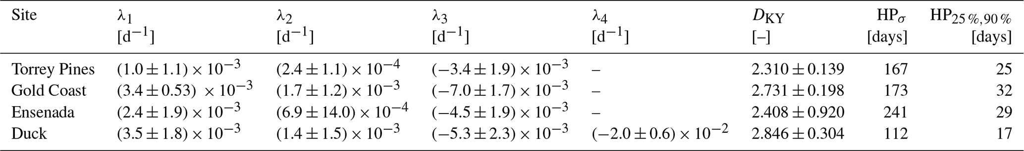
Table 6 Lyapunov exponents, Kaplan–Yorke dimension and Horizons of Predictability (HP) for the autonomous GPoM models identified at each site. Positive λ₁ indicates sensitivity to initial conditions, near zero λ₂ correspond to the direction of the flow, negative λ₃ and λ₄ reflect phase-space contraction (i.e. attractor boundedness). Lyapunov uncertainties were obtained by repeating the Lyapunov spectrum calculation from 10 initial states sampled along the numerically integrated attractor after transient removal, and reporting the mean ± standard deviation across these repeated estimates. The deterministic horizon (HP_σ) corresponds to the time when the mean RMS error equals the natural variability (1σ), here typically on semi-annual scales, indicating that the model retains the large-scale seasonal shoreline–sandbar dynamics. In contrast, the probabilistic horizon (HP_{25 %,90 %}) marks the time when 90 % of runs exceed a 25 % relative error, revealing rapid trajectory divergence and high sensitivity to initial conditions. Together, they show that the models preserve the global morphodynamic structure but offers forecasting ability at short time scale, as, the annual forcing imprint remain consequent within the morphological evolutions.

The Kaplan–Yorke dimension (Kaplan and Yorke, 1979) was obtained as:

$$\begin{array}{}\text{(14)}& \begin{array}{rl}{D}_{\text{KY}}=& j+{\displaystyle \frac{{\sum }_{i=\mathrm{1}}^j{\mathit{\lambda }}_i}{\left|{\mathit{\lambda }}_{j+\mathrm{1}}\right|}},\\ & \text{ where }j=max\left\{n:\sum _{i=\mathrm{1}}^n{\mathit{\lambda }}_i>\mathrm{0}\right\}.\end{array}\end{array}$$

All calculations were performed on the numerically integrated models after transient removal. The leading Lyapunov exponents (λ₁>0) confirm that all 4 systems present a high sensitivity to the initial conditions which, associated with the determinism guarantied by the obtained equations, provides a first argument for chaos (Table 6). This implies finite predictability horizons on the order of months to years, in line with observed study sites shoreline–sandbar main variability. The total divergence (${\sum }_i{\mathit{\lambda }}_i<\mathrm{0}$) indicates that the systems remain globally dissipative, with attractor contraction typical of bounded physical processes. The robustness of the underlying model structure to preprocessing choices (e.g., smoothing window length or embedding configuration) was verified through repeated runs with perturbed parameters (Sect. 2.5), providing indirect support for the stability of the inferred Lyapunov spectra.

The non-integer values of the Kaplan–Yorke dimensions ([2.3–2.8]) confirm the fractal nature of these attractors, implying scale-invariant structures and self-similar organization within the coupled shoreline–sandbar dynamics, and provide another argument for chaos. The dimensions obtained here are all quite high compared with the strongly dissipative chaos commonly observed in systems such as the paradigmatic Lorenz-1963 or Rössler-1976 models, whose dimension does not exceed 2.06. Very few continuous systems with fractal dimension greater than 2.10 were identified in the early development of chaos, whose lower dynamical dissipation gives them a characteristic foliated structure (Lorenz, 1984; Langford, 1984). From this perspective, the results obtained here are of particular interest because they confirm that this type of dynamics can also be extracted directly from real-world observational data.

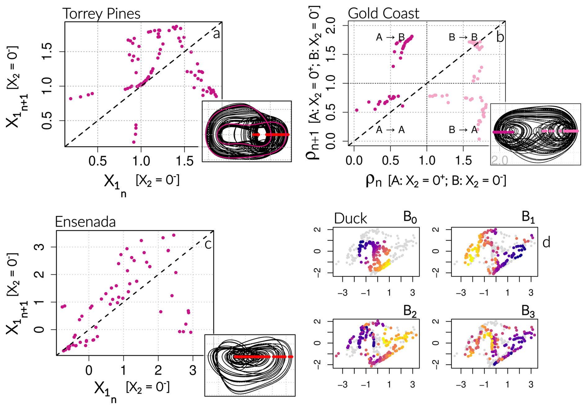
Figure 7 First-return maps or Poincaré sections computed for the 4 reconstructed systems. (a–c) Each dot corresponds to a successive intersection of the trajectory with the Poincaré section, providing a discrete sampling of the underlying continuous flow. The corresponding Poincaré section is overlaid (red dots for Torrey Pines and Ensenada, shade of pink for Gold Coast) on a two-dimensional representation of each attractor within each subpanel. (a) First-return map computed by applying dynamical noise during model integration in order to prevent the trajectory from falling into the period-2 basin normally reached in case of noise-free run (pink cycle within the subpanel). (b) First-return map computed for 2 distinct branches of the attractor (branch A: dark pink; branch B: light pink). (d) Poincaré section projected onto the (X₁,X₃) plane. B₀ denotes the initial neighborhood selected within the section, and B_i ($i=\mathrm{1},\mathrm{2},\mathrm{3}$) its successive images under the first-return map. Because the reconstructed Duck attractor has 4 embedding dimensions, colored markers are used to track the deformation and transport of B₀ across iterations, allowing the local geometry of the attractor to be visualized despite the two-dimensional projection.

To analyze the organization of the reconstructed attractors, Poincaré sections were extracted; from which first return maps were computed (Fig. 7a–c). Within the figure, each point corresponds to a successive intersection of the trajectory with the section, producing a discrete sampling of the continuous flow. This representation highlights how the flow stretches, folds, and squeezes from one passage to the next, making the underlying invariant structure directly visible. For a basic periodic orbit, the section would collapse into a single point, while quasi-periodic dynamics would produce a smooth closed curve. In contrast, deterministic chaos yields discontinuous but characteristic structured patterns of points. In the most common case, this organization can take an inverted-U shape crossing the median, as is the case for the logistic map (May, 1976), reflecting a single folding process that generates 2 distinct branches from a single branch at each iteration. More branches may be generated, leading to a multimodal distribution of points with multiple crossings of the median. Some situations may require several Poincaré sections of the same attractor to obtain a proper map-based description of the underlying structure. Branches may be clearly visible under strongly dissipative conditions, in which each branch corresponds to a single line, but are more difficult to depict under weakly dissipative conditions (as is the case here), because each branch can exhibit a thick, foliated structure.

At Torrey Pines, the trajectory was found to converge toward a stable period-two orbit after a very long transient. The complicated dynamics observed in the model phase portraits (Fig. 3) is therefore only metastable, although it may be easily triggered by perturbations. The Lyapunov exponents (for which the uncertainty in λ₁ is comparable in magnitude to the estimate itself) and the Kaplan–Yorke dimension (D_KY≈ 2.31; see Table 6) were estimated over this transient and thus characterize the associated dynamics, corresponding to metastable, weakly dissipative chaos. In order to represent the structure of this metastable transient, the first-return map was constructed by adding dynamical noise ($\mathit{ϵ}={\mathrm{10}}^{-\mathrm{5}}\times {\mathit{\sigma }}_{X_{\mathrm{1}}}$, with ${\mathit{\sigma }}_{X_{\mathrm{1}}}$ the standard deviation of the variable X₁) during model integration to prevent the trajectory from falling into the stable periodic orbit obtained in the noise-free integration case; enabling to reveal the underlying deterministic structure (Fig. 7a). The resulting map clearly exhibits a structure with an inverted-U shape characteristic of chaos. Its foliation reveals the folding of at least 2 main branches, possibly more.

At Gold Coast, the attractor is organized inside a genus-3 torus, which requires defining 2 Poincaré sections for a proper description (Rosalie and Letellier, 2014). The 2 sections were defined on the surface X₂=0 (see (Fig. 7b): the left one (A), on the interval $X_{\mathrm{1}}\in [-\mathrm{2},-\mathrm{0.5}]$, corresponding to a positive crossing ($X_{\mathrm{2}}={\mathrm{0}}^{+}$), and the right one (B), on the interval $X_{\mathrm{1}}\in [\mathrm{0},\mathrm{2}]$, corresponding to a negative crossing ($X_{\mathrm{2}}={\mathrm{0}}^{-}$). To reconstruct the first-return map, these 2 sections were assembled using a single coordinate axis. A decreasing orientation was defined for section A as: ${\mathit{\rho }}_A=(-\mathrm{0.5}-X_{\mathrm{1}})/\left(\mathrm{1.5}\right)$, while an increasing orientation was defined for section B as: ${\mathit{\rho }}_B=\mathrm{1}+X_{\mathrm{1}}/\mathrm{2}$, yielding a unified return interval $\mathit{\rho }\in [\mathrm{0},\mathrm{2}]$. The global return map ${\mathit{\rho }}_{n+\mathrm{1}}=\mathcal{P}\left({\mathit{\rho }}_n\right)$ thus explicitly resolves transitions within and between the different parts of the attractor, with the 4 quadrants of the map corresponding to A→A; A→B; B→A and B→B transitions. In agreement with the organization of the attractor observed in phase space (Fig. 3), the map confirms the presence of the 4 possible transitions (A→A; A→B; B→A; and B→B), indicating that the dynamics recurrently explores both parts of the attractor. The double-slash shape observed in the A→B region corresponds to a three-branch folding structure, but here with the middle branch missing.

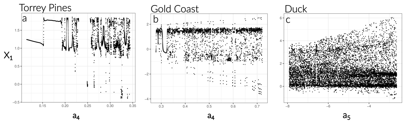
Figure 8 X₁ bifurcation diagram for 3 of the 4 sites. (a b) Torrey Pines and Gold Coast for the term $a_{\mathrm{4}}{X}_{\mathrm{2}}^{\mathrm{2}}{X}_{\mathrm{3}}$ and (c) Duck for the term $a_{\mathrm{5}}{X}_{\mathrm{2}}^{\mathrm{3}}$ within the $\dot{X_{\mathrm{2}}}$ equation when varying a_i from 0.5 to 1.5 times its original value for 5000 runs over 10 years. The X₁ local maxima over the last 300 d of each run are then scattered. For Gold Coast and Duck, transients have been removed, whereas the stable regime at Torrey Pines takes approximately 10 years to be established; consequently, its bifurcation diagram explores the complexity of the transient dynamics.

At Ensenada, the first-return map (Fig. 7c) is organized along a foliated bend revealing at least 2 distinct folding branches that provide a strong argument for chaos. The foliated structure is characteristic of a weakly dissipative chaotic attractor (D_KY=2.4). The attractor involves an extremely thin central branch on which all the trajectories loop at the bottom and pass through the attractor before reemerging and separating at the top (Fig. 3). This structure is similar to the “cord attractor” discovered in 2011 (Letellier and Aguirre, 2012), although here the thin central cord is completely bent within the attractor, which may make the detailed analysis of this attractor's structure particularly challenging. Especially, the large uncertainty on D_KY (±0.920) reflects strong variability in the local expansion rates along the cord-like attractor structure, whose thin central branch may produces intermittent near-zero contributions to the spectrum.

The case of Duck is even more demanding as analyzing the structure of chaotic attractors becomes a hard problem when their dimension is larger than 3 (Gilmore and Lefranc, 2002; Letellier and Gilmore, 2013). Few techniques developed to investigate their structure (Mindlin and Gilmore, 1992; Gilmore and Lefranc, 2002; Mangiarotti, 2014). Among these, recent studies have reported several promising results using homology-based approaches (Charó et al., 2022; Sciamarella and Charó, 2024; Mosto et al., 2024a). However, extracting the topological structure of chaotic attractors remains a challenging problem in many cases. In particular, for systems exhibiting weakly dissipative chaos, as in this study, the thick structure of their attractors makes it difficult to reduce them to a flat template. Hence, the color tracer mapping method developed to characterize foliated structures provides an alternative, particularly as it can also be applied to toroidal chaos (including weakly dissipative cases), as well as hyperchaotic attractors and maps (Mangiarotti et al., 2023; Rosalie and Mangiarotti, 2025). This technique consists of applying color tracers at a chosen Poincaré section and examining their reorganization between successive iterations. The tracers allow one to follow the evolution of a small neighborhood of points across successive returns. This technique was applied to investigate the presence of folding and stretching within the Poincaré section of the Duck attractor (Fig. 7d), which is very thick as consistently shown by an estimated dimension close to 3 (D_KY=2.85). Starting from an initial state B₀, points are first selected within a compact region of the Poincaré section and colored according to their position along the first principal component obtained from a local Principal Component Analysis (Abdi and Williams, 2010). Hence, The covariance matrix of these coordinates is decomposed, and the first principal component (i.e., the direction capturing the largest variance within B₀) is extracted. Each point is then projected onto this axis, yielding a scalar value that is linearly mapped to a continuous color scale. This color assignment provides a spatially coherent label within B₀: points that are close together and share a similar position along the dominant axis of the neighborhood receive similar colors, while points at opposite ends of the neighborhood receive contrasting colors. As the dynamics are iterated forward, this labeling is preserved, so that the geometric deformation of B₀ (stretching, folding, and squeezing) becomes directly readable from the reorganization of colors in B₁, B₂, and B₃. The images of B₀ at successive states B₁, B₂, and B₃ reveal (1) very strong stretching: initially confined to a localized region in B₀, the colors spread over almost the entire Poincaré section after a single iteration (B₁); (2) strong mixing, since after several iterations, points carrying very distant colors in B₀ come into contact in B₃. This behavior results from the combined action of folding (where the color gradient remains locally consistent almost everywhere between successive iterations, as illustrated in B₁), and squeezing, evidenced by the local compaction of trajectories in specific regions of the section.

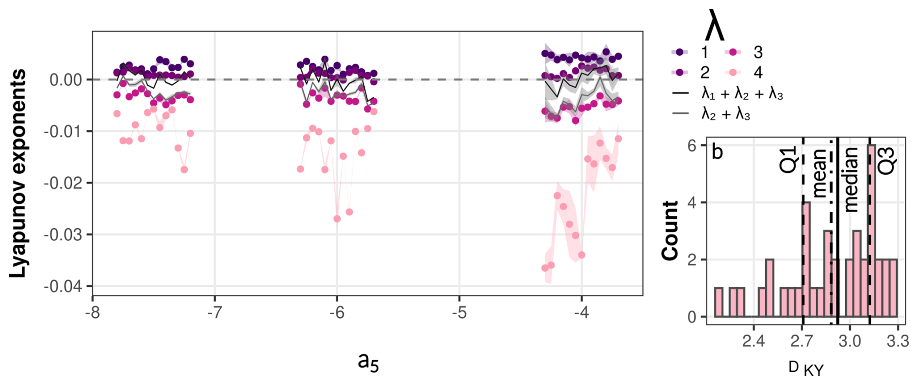
Figure 9 Lyapunov analysis of Duck as a function of various ranges of the control parameter a₅. (a) Lyapunov spectrum estimated after transient removal. Numerical robustness of the estimates is estimating by repeated computations (K=5) using, each time, slightly perturbed initial conditions. The resulting uncertainty ranges are shown through the color shaded envelopes. Thin black and gray lines show the sums λ₂+λ₃ and ${\mathit{\lambda }}_{\mathrm{1}}+{\mathit{\lambda }}_{\mathrm{2}}+{\mathit{\lambda }}_{\mathrm{3}}$, used to diagnose the proximity to a regime with 2 expanding directions and to highlight regions of weak dissipation, respectively. Gray bands indicate ± 1 standard deviation of the ensemble. (b) Distribution of the Kaplan–Yorke dimension D_KY computed from the Lyapunov spectrum for all tested values of a₅. The dimension predominantly lies between approximately 2.7 and 3.3, with a median value close to 3.

Together with the positive first Lyapunov exponent and the fractal dimension, and supported by the deterministic nature guaranteed by the reconstructed equations, the first-return maps and the color tracer mapping provide dynamical, geometrical, and topological evidence of weakly dissipative chaos at the 4 sites either as a transient dynamics recurrently triggered by external forcing (Torrey Pines) or as permanent dynamics (at the other 3 sites). This implies that shoreline–sandbar systems exhibit internal dynamics prone to chaotic behavior, structured by morphodynamic feedback loops and weak dynamical dissipation. While physical energy inputs associated with wave forcing are large, the effective dissipation of the reconstructed dynamics remains weak, so that the system is not strongly damped and retains long-term memory and sensitivity to small perturbations.

The bifurcation diagrams (Fig. 8), obtained by slowly varying the coefficient values of specific terms, were also reconstructed. They present contrasted behaviors over the studied sites. The classical doubling period cascade was not observed at any of them, which may be an indication of toroidal chaos, as observed in low-dimensional models of atmosphere dynamics.

At Torrey Pines, the bifurcation diagram is characterized by abrupt alternation of periodic, either period-1 (single value e.g. at $\mathrm{0.11}<a_{\mathrm{4}}<\mathrm{0.18}$ with an abrupt change of amplitude at a₄=0.155), or more rarely period-2 (two values e.g. at $\mathrm{0.28}<a_{\mathrm{4}}<\mathrm{0.29}$) dynamics, and chaotic (complex distribution of points, in the ranges [0.21;0.22], [0.26;0.27], [0.31;0.33]) and organized around 2 main regions: around X₁=1.25 and $X_{\mathrm{1}}\in [\mathrm{1.0};\mathrm{1.25}]$.

An organization around 2 main layers is also observed at Gold Coast, but the dynamic appears periodic only in very localized regions (e.g. in $\mathrm{0.3}<a_{\mathrm{4}}<\mathrm{0.32}$) whereas the dynamic is chaotic elsewhere.

At Ensenada, a well-defined bifurcation diagram could not be obtained across the explored parameter range, reflecting some properties of the system. As a cord-like attractor organized around a thin central branch acting as a overall bottleneck for the flow, its structure is very sensitive to parameter perturbations (i.e., small variations in parameter during bifurcation search may lead to divergence, or collapse onto simple periodic orbit without passing through bifurcation sequences). Moreover, one could argue a technical reason explaining the non finding of a bifurcation diagram due to the model structure recovered with GPoM. In the case of Ensenada, the sandbar equation contains a strongly nonlinear term $b_{\mathrm{4}}{X}_{\mathrm{3}}^{\mathrm{2}}$ with an unusually large coefficient (b₄=3.61×10²), which provides a dominant restoring contribution to the sandbar dynamics. As the existence of the attractor depends on a precise balance between this large term and the remaining coupling structure, this makes the system dynamically fragile under parameter perturbations in a way that is not observed at the other sites. However, this does not affect the evidence for chaos at this site, which rests independently on the positive Lyapunov exponent, the fractal attractor dimension, and the topological structure of the first-return map.

Finally, at Duck, the dynamics were found chaotic on the whole parameter window ($-\mathrm{7.8}<a_{\mathrm{5}}<-\mathrm{2.5}$). Because the model obtained at this site is four-dimensional, the very high value of D_KY suggest a proximity to hyperchaos, which requires 2 positive Lyapunov exponents (${\mathit{\lambda }}_{\mathrm{1}}>{\mathit{\lambda }}_{\mathrm{2}}>{\mathit{\lambda }}_{\mathrm{3}}=\mathrm{0}\gg {\mathit{\lambda }}_{\mathrm{4}}$), (Rössler, 1979, 1983).

To investigate this question, the Lyapunov spectrum was estimated in 3 subwindows of the bifurcation diagram, around a₄=7.75, −6, and −3.9. Figure 9a shows the individual Lyapunov exponents of the Duck system as a function of the control parameter a₅ after transient removal. The largest exponent λ₁ is strictly positive over the entire parameter range, indicating robust chaotic dynamics. The second exponent λ₂ remains close to zero almost everywhere and significantly smaller than λ₁, while λ₃ and λ₄ are negative. In continuous autonomous systems, one Lyapunov exponent must equal zero, corresponding to the direction of the flow. Since numerical algorithms do not explicitly isolate this direction, the neutral exponent may be mixed with nearby weakly stable or unstable directions. As a result, particular care must be taken when interpreting a second small positive exponent as evidence for hyperchaos. To address this issue, we additionally show the sums λ₂+λ₃ and ${\mathit{\lambda }}_{\mathrm{1}}+{\mathit{\lambda }}_{\mathrm{2}}+{\mathit{\lambda }}_{\mathrm{3}}$. Negative values of λ₂+λ₃ are obtained almost everywhere indicating that λ₂ is closer to zero and corresponds to the flow direction (λ₂≡0). Positive values of λ₂+λ₃ indicate λ₃ is closer to zero and corresponds to the flow direction (λ₃≡0). The former condition is observed almost everywhere while the latter one is observed only very locally in parameter space ($a_{\mathrm{5}}=-\mathrm{7.75}$ and −3.9), suggesting that the dynamical system may reach hyperchaotic regimes under small configuration changes and that, overall, the observed dynamics operates close to hyperchaos. The partial sum ${\mathit{\lambda }}_{\mathrm{1}}+{\mathit{\lambda }}_{\mathrm{2}}+{\mathit{\lambda }}_{\mathrm{3}}$ provides an estimate of the effective dynamical dissipation and highlights parameter regions where the dynamics is weakly dissipative. As shown, this sum is often close to or above zero for the explored parameter values, supporting the interpretation of a low-dimensional, weakly dissipative chaotic attractor. The associated D_KY distribution mostly lies between 2.7 and 3.3 (Fig. 9b), with a median value close to 3. While D_KY>3 is not sufficient to establish hyperchaos, it provides geometric support for the interpretation that the Duck system operates near the transition between chaotic and hyperchaotic regimes. To conclude, the Duck system exhibits robust chaos across the explored parameter range and displays signatures consistent with proximity to hyperchaotic dynamics, although the identification of a fully developed hyperchaotic regime is limited to narrow regions of parameter space.

In addition, the predictability horizons (HP) were evaluated (Table 6) from the growth of the prediction error over an ensemble of 50 initial conditions using 2 complementary criteria (See Figs. S1–12 in the Supplement). The first, HP_σ, corresponds to the time at which the mean RMSE reaches 1 standard deviation of the observed signal, marking the loss of dynamical coherence between simulated and observed trajectories. The second, HP_{25 %,90 %}, follows the probabilistic approach proposed by Mangiarotti and Le Jean (2023), defined as the horizon at which 90 % of the ensemble members exhibit a relative error exceeding 25 % of the signal amplitude. Across sites, both criteria yield consistent results, with HP_σ typically of the order of half a year and HP_{25 %,90 %} around 1 month. This dual structure of predictability indicates that the reconstructed models retain short-term skill for about one monthly cycle, while maintaining partial dynamical consistency over the semi-annual timescale. The semi-annual predictability horizon is consistent with the dominant systems' annual periodicity, over which the autocorrelation of the principal morphological proxies of beach evolution remains significant for approximately half a cycle (Reeve et al., 2014). This suggests that the models reproduce the internal oscillatory memory of the system, while their forecast skill remains limited in the absence of external forcing driving the dynamics. Conversely, the shorter HP_{25 %,90 %} reflects the timescale beyond which small phase errors accumulate to produce significant amplitude mismatches, even though the overall trajectory remains within the correct attractor. Beyond their diagnostic value, these horizons also serve as a model validity assessment metric. As illustrated in Figs. C1–C4, 10 runs initialized from distinct initial conditions sampled across the observed phase space (each perturbed by 2 %) show that the reconstructed models satisfactorily reproduce the observed trajectories over their respective predictability horizons, while performance expectedly varies with the starting point. This provides direct evidence against overfitting: a model that had merely memorized the training trajectory would diverge rapidly from observations when initialized from unvisited regions of the phase space. The consistent, if imperfect, agreement across multiple initial conditions (supported by estimated predictability horizons) therefore confirms that the reconstructed dynamics capture the intrinsic memory and global attractor structure of the coastal system, rather than a single realization of it.

Taken together, these results demonstrate that all 4 systems operate within a chaotic regime. First, the 4 dynamics can be approximated by low-dimensional ordinary differential equations, which are a strong argument in favor of determinism and a necessary condition for chaos. The solutions of these equations converge toward attractors of nontrivial structure, characterized by a strong sensitivity to initial conditions (λ₁>0) and finite predictability (Table 6), which constitutes another necessary condition for chaos. The resulting attractors exhibit a fractal structure with single or multiple foldings, a hallmark of chaotic dynamics. More specifically, the attractors display a thick structure, a property rather rarely encountered in chaotic systems, as reflected by their Kaplan–Yorke dimensions (2.31 < D_KY < 2.85). Such dynamics establish the bridge between short-term unpredictability and long-term structural coherence, consistent with the self-regulated nature of coastal morphodynamic systems driven by processes spanning a broad range of spatiotemporal scales, from storm events to climatic modulations.

4 Discussion

This study provides direct evidence that the coupled shoreline–sandbar system behaves as a low-dimensional deterministic dynamical system across a wide range of morphodynamic settings. The ability of the reconstructed models to reproduce both the global organization of the phase space (characteristic oscillatory loops, asymmetries) and the multiscale spectral structure of the observations indicates that the essential dynamics are captured by a small number of interacting degrees of freedom. This supports the view that sandy beaches, despite being continuously forced by waves and other environmental variables, can organize their response through deterministic internal dynamics. Importantly, the models are fully autonomous: no external forcing is prescribed, yet the reconstructed dynamics retain realistic amplitudes, oscillatory behavior, and broadband red spectra. This implies that the influence of external drivers is effectively embedded within the internal state variables, and that the shoreline–sandbar system integrates forcing over time through its own nonlinear structure. This formulation does not imply that external forcing is negligible, but rather that its morphological imprint persists over sufficiently long timescales (e.g., seasonal), allowing the model to capture its memory within the system, together with the variability associated with purely internal dynamics such as feedbacks or hysteresis.

A potential limitation concerns extreme events, such as coastal storms, which may significantly disrupt the system and induce rapid excursions of shoreline and sandbar positions (Eichentopf et al., 2019; Criado Sudau et al., 2023; Medellin et al., 2024). Here, however, and without generalizing to all beaches, the dominant dynamics observed at the studied sites drive the system back toward a characteristic range of variability, making it amenable to an effective low-dimensional description over the considered temporal window. Hence, the reconstructed models should be interpreted as effective dynamical representations of a given morphodynamic regime sampled over the observation period. As such, they are not expected to remain invariant under substantial changes in forcing statistics, such as a increase in storm frequency or intensity driven by climate change (Intergovernmental Panel On Climate Change (Ipcc), 2022). In such cases, changes in the effective parameters and coupling structure may be anticipated. One straightforward extension of the present framework would therefore consist in regime-dependent reconstruction by refitting the models over different periods to quantify how the inferred feedback structure, attractor geometry, and dynamical invariants evolve with changes in storm climate. A complementary and more physically explicit approach would be to extend the formulation toward non-autonomous models by including external covariates (e.g., storm indices, wave-energy metrics) as explicit inputs. This would enable controlled sensitivity experiments to assess how specific changes in forcing statistics modulate the internal shoreline–sandbar dynamics, the feasibility of which has been previously demonstrated using this data-driven approach for CO₂ concentrations in cave systems (Sáez et al., 2024).

Across all sites, the reconstructed equations reveal that shoreline and sandbar dynamics are mutually coupled, rather than hierarchically driven. The shoreline does not simply respond passively to sandbar migration, nor does the sandbar act as an independent buffer; instead, both components participate in closed feedback loops whose strength and sign depend on the system state. For Torrey Pines and Ensenada, the dominant coupling corresponds to a seasonal exchange mechanism in which offshore sandbar migration accompanies shoreline retreat, while onshore migration promotes recovery. This behavior is consistent with a variable surf-zone hydrodynamic energy dissipation length that adapts to wave climate, producing bounded oscillations around a stable mean state. At Gold Coast, the coupling differs qualitatively: shoreline and sandbar positions tend to evolve coherently, indicating a translation-dominated regime in which the surf-zone geometry is conserved. The Duck system, operating within a regime close to hyperchaos, departs markedly from the other sites. Its dynamics are dominated by velocity-dependent nonlinear interactions, with no direct restoring term acting on shoreline position. Sandbar dynamics exhibit intrinsic instability and strong sensitivity to shoreline motion, resulting in a highly complex attractor structure. This supports field-based interpretations of Duck as a system with strong memory effects and path dependence, where antecedent morphology conditions subsequent evolution (Anderson et al., 2023). These results indicate that shoreline–sandbar coupling is not universal in form, but universal in presence: internal feedbacks are always active, yet their organization depends on the morphodynamic regime.

Therefore, relating these results to established coastal morphodynamic classifications (Wright and Short, 1984; Masselink and Short, 1993; Castelle and Masselink, 2023) provides a consistent framework to draw implications from the present results. The conclusion inferred here from the analysis of autonomous models derived from observational data shows that part of the shoreline and sandbar variability should be interpreted as internally generated, rather than as a direct response to short-term fluctuations in external forcings, even if their imprint on morphological evolution remains dominant at the seasonal scale. This presents implications for both modeling and signal interpretation, since phenomena that are part of the internal dynamics of sandy beaches (lags, feedback loops, morphodynamic turbulence, and so on) necessarily account for a non-negligible fraction of the variability, which process-based models that neglect internal nonlinear feedbacks may misattribute to stochastic forcing or parameter uncertainty. The low dimensionality of the reconstructed systems further implies that shoreline–sandbar dynamics may be amenable to reduced-order modeling approaches that explicitly account for nonlinear coupling and instability, rather than relying solely on equilibrium frameworks (Dean, 1991; Yates et al., 2009; Davidson et al., 2013). These models describe shoreline change as a relaxation process toward a forcing-dependent equilibrium where wave energy enters as an explicit external driver. These models are non-autonomous, one-dimensional in state space, and structurally limited to monotonic decay toward equilibrium. Hence, they cannot, by construction, produce self-sustained oscillations, limit cycles, or sensitivity to initial conditions. Moreover, the sandbar does not appear as an independent dynamical degree of freedom in their shared framework. The GPoM-reconstructed systems therefore differ in that they are fully autonomous, yet able to sustain realistic oscillatory behavior and broadband red spectra, while incorporating sandbar position as an active state variable whose coupling with shoreline dynamics governs both the sign and the nonlinearity of the feedback structure.

While the present models are not intended as long-term predictive tools and may not meet engineering performance criteria based on trajectory-level accuracy, they provide a compact dynamical reference for assessing the structure, stability, and coupling mechanisms represented in more complex or process-based models. Moreover, the existence of site-specific coupling structures suggests that coastal typologies based solely on external forcing or mean morphology may be incomplete. Internal dynamics and feedback organization appear to play a central role in controlling both variability and resilience of the beach system.

Finally, the estimated Lyapunov spectra imply finite predictability horizons, typically on the order of months to a few years, consistent with observed limits in shoreline forecasting skill. A recent large-scale benchmarking study have shown that shoreline prediction skill saturates at levels comparable to observational uncertainty, regardless of model complexity (Mao et al., 2025). While often attributed to data limitations, our results suggest that this saturation may also reflect an intrinsic loss of predictability associated with low-dimensional chaotic dynamics. This result provides a dynamical explanation for why long-term prediction of shoreline position remains challenging even when wave climate statistics are well characterized: beyond a certain horizon, forecast uncertainty grows exponentially due to internal instability, not because of incomplete forcing information. From this perspective, the shoreline–sandbar system behaves as a chaotic oscillator: its dynamics are structured and deterministic, yet long-term trajectories are inherently unpredictable. This reconciles the apparent contradiction between reproducible seasonal patterns and large interannual variability observed in many sandy beaches.

5 Conclusions

This study demonstrates that sandy shoreline–sandbar systems, despite strong environmental variability, can be represented by low-dimensional deterministic models exhibiting chaotic dynamics. Using global polynomial modeling applied to multi-year satellite-derived observations, we reconstructed autonomous equations that reproduce the essential coupling between shoreline and sandbar motion. The models reveal bounded, chaotic attractors with finite predictability horizons, highlighting the coexistence of short-term irregularity and long-term structural organization.

Across sites, the nonlinear feedbacks controlling shoreline acceleration and sandbar migration define distinct regimes (from dissipative to intermittently unstable oscillators) governed by the sign and strength of sandbar-related coupling terms. The emergence of chaos thus reflects an intrinsic property of morphodynamic systems where energy exchanges between shoreline and sandbar sustain self-regulated variability.

Despite these advances, several limitations remain. The reconstructed models are not intended to provide engineering-grade predictive performance, nor to reproduce individual events or trajectories with high accuracy. Their limited predictive skill at the trajectory level reflects both the reduced-order nature of the approach and the intrinsic sensitivity of the system. Furthermore, the contribution of external forcing is not explicitly considered in this study. Temporal sampling and noise in satellite observations also constrain the precision of model coefficients and Lyapunov estimates. Furthermore, the analysis is restricted to 3–4-dimensional systems, which may overlook higher-order or non-local interactions present in real coastal dynamics.

Future work should focus on coupling autonomous data-driven dynamical reconstruction and climate forcing to assess how external variability (waves, storms, sea-level rise) interacts with intrinsic shoreline–sandbar dynamics. Expanding the analysis to other coastal settings would help assess for the variety of these nonlinear behaviors.

Overall, this study provides a novel dynamical framework to interpret shoreline evolution as a self-regulated, chaotic system. It bridges satellite observation and system dynamics theory, offering new tools to assess the stability, predictability, and resilience of sandy coasts under changing environmental conditions.

Appendix A: Model simplification details

A1 Torrey Pines

Considering only the terms with a variance of Var_eq≥ 10 % (see Table 2) leads to:

$$\begin{array}{}\text{(A1)}& \left\{\begin{array}{ll}{\dot{X}}_{\mathrm{1}}& =X_{\mathrm{2}}\\ {\dot{X}}_{\mathrm{2}}& =-a_{\mathrm{7}}{X}_{\mathrm{1}}^{\mathrm{3}}+a_{\mathrm{3}}{X}_{\mathrm{2}}^{\mathrm{3}}-a_{\mathrm{6}}{X}_{\mathrm{1}}^{\mathrm{2}}{X}_{\mathrm{3}}\\ {\dot{X}}_{\mathrm{3}}& =-b_{\mathrm{3}}{X}_{\mathrm{2}}-b_{\mathrm{4}}{X}_{\mathrm{3}}^{\mathrm{3}}.\end{array}\right.\end{array}$$

Defining the second order derivatives, we get:

$$\begin{array}{}\text{(A2)}& \left\{\begin{array}{ll}{\ddot{X}}_{\mathrm{1}}& =-a_{\mathrm{7}}{X}_{\mathrm{1}}^{\mathrm{3}}+a_{\mathrm{2}}{X}_{\mathrm{3}}^{\mathrm{3}}-a_{\mathrm{6}}{X}_{\mathrm{1}}^{\mathrm{2}}{X}_{\mathrm{3}}\\ {\ddot{X}}_{\mathrm{3}}& =-b_{\mathrm{3}}{\ddot{X}}_{\mathrm{1}}-\mathrm{3}{b}_{\mathrm{4}}{X}_{\mathrm{3}}^{\mathrm{2}}{\dot{X}}_{\mathrm{3}},\end{array}\right.\end{array}$$

and then:

$$\begin{array}{}\text{(A3)}& \left\{\begin{array}{ll}{\mathit{A}}_{\mathrm{1}}& =-a_{\mathrm{7}}{X}_{\mathrm{1}}^{\mathrm{2}}{\mathit{X}}_{\mathrm{1}}+a_{\mathrm{2}}{X}_{\mathrm{3}}^{\mathrm{2}}{\mathit{X}}_{\mathrm{3}}-a_{\mathrm{6}}{X}_{\mathrm{1}}^{\mathrm{2}}{\mathit{X}}_{\mathrm{3}}\\ {\mathit{A}}_{\mathrm{3}}& =-b_{\mathrm{3}}{\mathit{A}}_{\mathrm{1}}-\mathrm{3}{b}_{\mathrm{4}}{X}_{\mathrm{3}}^{\mathrm{2}}{\mathit{V}}_{\mathrm{3}},\end{array}\right.\end{array}$$

with A_i and V_i the sand mass acceleration and speed, respectively. Under the hypothesis that both masses are equal (m₁=m₃), we can view the problem as the force applied to the sand masses as:

$$\begin{array}{}\text{(A4)}& \left\{\begin{array}{ll}{\mathit{F}}_{\mathrm{1}}& =-a_{\mathrm{7}}{X}_{\mathrm{1}}^{\mathrm{2}}{\mathit{X}}_{\mathrm{1}}+a_{\mathrm{2}}{X}_{\mathrm{3}}^{\mathrm{2}}{\mathit{X}}_{\mathrm{3}}-a_{\mathrm{6}}{X}_{\mathrm{1}}^{\mathrm{2}}{\mathit{X}}_{\mathrm{3}}\\ {\mathit{F}}_{\mathrm{3}}& =-b_{\mathrm{3}}{\mathit{F}}_{\mathrm{1}}-\mathrm{3}{b}_{\mathrm{4}}{X}_{\mathrm{3}}^{\mathrm{2}}{\mathit{V}}_{\mathrm{3}}.\end{array}\right.\end{array}$$

A2 Gold Coast

Considering only the terms with a variance of Var_eq≥ 10 % (see Table 3) leads to:

$$\begin{array}{}\text{(A5)}& \left\{\begin{array}{ll}{\dot{X}}_{\mathrm{1}}& =X_{\mathrm{2}}\\ {\dot{X}}_{\mathrm{2}}& =-a_{\mathrm{9}}{X}_{\mathrm{1}}^{\mathrm{3}}+a_{\mathrm{5}}{X}_{\mathrm{1}}-a_{\mathrm{1}}{X}_{\mathrm{3}}\\ {\dot{X}}_{\mathrm{3}}& =b_{\mathrm{3}}{X}_{\mathrm{2}}-b_{\mathrm{5}}{X}_{\mathrm{1}}^{\mathrm{2}}.\end{array}\right.\end{array}$$

Defining the second order derivatives, we get:

$$\begin{array}{}\text{(A6)}& \left\{\begin{array}{ll}{\ddot{X}}_{\mathrm{1}}& =-a_{\mathrm{9}}{X}_{\mathrm{1}}^{\mathrm{3}}+a_{\mathrm{5}}{X}_{\mathrm{1}}-a_{\mathrm{1}}{X}_{\mathrm{3}}\\ {\ddot{X}}_{\mathrm{3}}& =b_{\mathrm{3}}{\ddot{X}}_{\mathrm{1}}-\mathrm{2}{b}_{\mathrm{5}}\dot{X_{\mathrm{1}}}{X}_{\mathrm{1}},\end{array}\right.\end{array}$$

and then:

$$\begin{array}{}\text{(A7)}& \left\{\begin{array}{ll}{\mathit{A}}_{\mathrm{1}}& =-a_{\mathrm{9}}{X}_{\mathrm{1}}^{\mathrm{2}}{\mathit{X}}_{\mathrm{1}}+a_{\mathrm{5}}{\mathit{X}}_{\mathrm{1}}-a_{\mathrm{1}}{\mathit{X}}_{\mathrm{3}}\\ {\mathit{A}}_{\mathrm{3}}& =b_{\mathrm{3}}{\mathit{A}}_{\mathrm{1}}-\mathrm{2}{b}_{\mathrm{5}}{X}_{\mathrm{1}}{\mathit{V}}_{\mathrm{1}},\end{array}\right.\end{array}$$

with A_i and V_i the sand mass acceleration and speed, respectively. Under the hypothesis that both masses are equal (m₁=m₃), we can view the problem as the force applied to the sand masses as:

$$\begin{array}{}\text{(A8)}& \left\{\begin{array}{ll}{\mathit{F}}_{\mathrm{1}}& =-a_{\mathrm{9}}{X}_{\mathrm{1}}^{\mathrm{2}}{\mathit{X}}_{\mathrm{1}}+a_{\mathrm{5}}{\mathit{X}}_{\mathrm{1}}-a_{\mathrm{1}}{\mathit{X}}_{\mathrm{3}},\\ {\mathit{F}}_{\mathrm{3}}& =b_{\mathrm{3}}{\mathit{F}}_{\mathrm{1}}-\mathrm{2}{b}_{\mathrm{5}}{X}_{\mathrm{1}}{\mathit{V}}_{\mathrm{1}}.\end{array}\right.\end{array}$$

A3 Ensenada

Considering only the terms with a variance of Var_eq≥ 10 % (see Table 4) leads to:

$$\begin{array}{}\text{(A9)}& \left\{\begin{array}{ll}{\dot{X}}_{\mathrm{1}}& =X_{\mathrm{2}}\\ {\dot{X}}_{\mathrm{2}}& =-a_{\mathrm{8}}{X}_{\mathrm{1}}^{\mathrm{3}}-a_{\mathrm{6}}{X}_{\mathrm{1}}^{\mathrm{2}}{X}_{\mathrm{3}}+a_{\mathrm{1}}{X}_{\mathrm{3}}\\ {\dot{X}}_{\mathrm{3}}& =-b_{\mathrm{3}}{X}_{\mathrm{2}}+b_{\mathrm{4}}{X}_{\mathrm{2}}^{\mathrm{3}}.\end{array}\right.\end{array}$$

Defining the second order derivatives, we get:

$$\begin{array}{}\text{(A10)}& \left\{\begin{array}{ll}{\ddot{X}}_{\mathrm{1}}& =-a_{\mathrm{8}}{X}_{\mathrm{1}}^{\mathrm{3}}-a_{\mathrm{6}}{X}_{\mathrm{1}}^{\mathrm{2}}{X}_{\mathrm{3}}+a_{\mathrm{1}}{X}_{\mathrm{3}}\\ {\ddot{X}}_{\mathrm{3}}& =-b_{\mathrm{3}}\ddot{X_{\mathrm{1}}}+\mathrm{3}{b}_{\mathrm{4}}{X}_{\mathrm{2}}^{\mathrm{2}}\dot{X_{\mathrm{2}}},\end{array}\right.\end{array}$$

and then:

$$\begin{array}{}\text{(A11)}& \left\{\begin{array}{ll}{\mathit{A}}_{\mathrm{1}}& =-a_{\mathrm{8}}{X}_{\mathrm{1}}^{\mathrm{2}}{\mathit{X}}_{\mathrm{1}}-a_{\mathrm{6}}{X}_{\mathrm{1}}^{\mathrm{2}}{\mathit{X}}_{\mathrm{3}}+a_{\mathrm{1}}{\mathit{X}}_{\mathrm{3}}\\ {\mathit{A}}_{\mathrm{3}}& =-b_{\mathrm{3}}{\mathit{A}}_{\mathrm{1}}+\mathrm{3}{b}_{\mathrm{4}}{X}_{\mathrm{2}}^{\mathrm{2}}{\mathit{A}}_{\mathrm{1}},\end{array}\right.\end{array}$$

with A_i and V_i the sand mass acceleration and speed, respectively. Under the hypothesis that both masses are equal (m₁=m₃), we can view the problem as the force applied to the sand masses as:

$$\begin{array}{}\text{(A12)}& \left\{\begin{array}{ll}{\mathit{F}}_{\mathrm{1}}& =-a_{\mathrm{8}}{X}_{\mathrm{1}}^{\mathrm{2}}{\mathit{X}}_{\mathrm{1}}-a_{\mathrm{6}}{X}_{\mathrm{1}}^{\mathrm{2}}{\mathit{X}}_{\mathrm{3}}+a_{\mathrm{1}}{\mathit{X}}_{\mathrm{3}},\\ {\mathit{F}}_{\mathrm{3}}& =-b_{\mathrm{3}}{\mathit{F}}_{\mathrm{1}}+\mathrm{3}{b}_{\mathrm{4}}{X}_{\mathrm{2}}^{\mathrm{2}}{\mathit{F}}_{\mathrm{1}}.\end{array}\right.\end{array}$$

A4 Duck

Considering only the terms with a variance of Var_eq≥ 10 % (see Table 5) leads to:

$$\begin{array}{}\text{(A13)}& \left\{\begin{array}{ll}{\dot{X}}_{\mathrm{1}}& =X_{\mathrm{2}}\\ {\dot{X}}_{\mathrm{2}}& =a_{\mathrm{4}}{X}_{\mathrm{2}}^{\mathrm{2}}{X}_{\mathrm{3}}-a_{\mathrm{5}}{X}_{\mathrm{2}}^{\mathrm{3}}-a_{\mathrm{11}}{X}_{\mathrm{1}}{X}_{\mathrm{2}}{X}_{\mathrm{4}}\\ & -a_{\mathrm{11}}{X}_{\mathrm{1}}{X}_{\mathrm{2}}^{\mathrm{2}}-a_{\mathrm{8}}{X}_{\mathrm{1}}{X}_{\mathrm{4}}^{\mathrm{2}}\\ {\dot{X}}_{\mathrm{3}}& =X_{\mathrm{4}}\\ {\dot{X}}_{\mathrm{4}}& =-c_{\mathrm{1}}{X}_{\mathrm{3}}^{\mathrm{3}}+c_{\mathrm{3}}{X}_{\mathrm{1}}.\end{array}\right.\end{array}$$

Defining the second order derivatives, we get:

$$\begin{array}{}\text{(A14)}& \left\{\begin{array}{ll}{\ddot{X}}_{\mathrm{1}}& =a_{\mathrm{4}}{X}_{\mathrm{2}}^{\mathrm{2}}{X}_{\mathrm{3}}-a_{\mathrm{5}}{X}_{\mathrm{2}}^{\mathrm{3}}-a_{\mathrm{11}}{X}_{\mathrm{1}}{X}_{\mathrm{2}}{X}_{\mathrm{4}}\\ & -a_{\mathrm{11}}{X}_{\mathrm{1}}{X}_{\mathrm{2}}^{\mathrm{2}}-a_{\mathrm{8}}{X}_{\mathrm{1}}{X}_{\mathrm{4}}^{\mathrm{2}}\\ {\ddot{X}}_{\mathrm{3}}& =-c_{\mathrm{1}}{X}_{\mathrm{3}}^{\mathrm{3}}+c_{\mathrm{3}}{X}_{\mathrm{1}},\end{array}\right.\end{array}$$

and then:

$$\begin{array}{}\text{(A15)}& \left\{\begin{array}{ll}{\mathit{A}}_{\mathrm{1}}& =a_{\mathrm{4}}{X}_{\mathrm{2}}^{\mathrm{2}}{\mathit{X}}_{\mathrm{3}}-a_{\mathrm{5}}{X}_{\mathrm{2}}^{\mathrm{2}}{\mathit{X}}_{\mathrm{2}}\\ & -a_{\mathrm{11}}{X}_{\mathrm{1}}{X}_{\mathrm{2}}{\mathit{X}}_{\mathbf{4}}-a_{\mathrm{11}}{\mathit{X}}_{\mathrm{1}}{X}_{\mathrm{2}}^{\mathrm{2}}-a_{\mathrm{8}}{\mathit{X}}_{\mathrm{1}}{X}_{\mathrm{4}}^{\mathrm{2}}\\ {\mathit{A}}_{\mathrm{3}}& =-c_{\mathrm{1}}{X}_{\mathrm{3}}^{\mathrm{2}}{\mathit{X}}_{\mathrm{3}}+c_{\mathrm{3}}{\mathit{X}}_{\mathrm{1}},\end{array}\right.\end{array}$$

with A_i and V_i the sand mass acceleration and speed, respectively. Under the hypothesis that both masses are equal (m₁=m₃), we can view the problem as the force applied to the sand masses as:

$$\begin{array}{}\text{(A16)}& \left\{\begin{array}{ll}{\mathit{F}}_{\mathrm{1}}& =a_{\mathrm{4}}{X}_{\mathrm{2}}^{\mathrm{2}}{\mathit{X}}_{\mathrm{3}}-a_{\mathrm{5}}{X}_{\mathrm{2}}^{\mathrm{2}}{\mathit{X}}_{\mathrm{2}}\\ & -a_{\mathrm{10}}{X}_{\mathrm{1}}{X}_{\mathrm{2}}{\mathit{X}}_{\mathbf{4}}-a_{\mathrm{11}}{X}_{\mathrm{2}}^{\mathrm{2}}{\mathit{X}}_{\mathrm{1}}-a_{\mathrm{8}}{X}_{\mathrm{4}}^{\mathrm{2}}{\mathit{X}}_{\mathrm{1}},\\ {\mathit{F}}_{\mathrm{3}}& =c_{\mathrm{1}}{X}_{\mathrm{3}}^{\mathrm{2}}{\mathit{X}}_{\mathrm{3}}+c_{\mathrm{3}}{X}_{\mathrm{1}}^{\mathrm{2}}{\mathit{X}}_{\mathrm{1}}.\end{array}\right.\end{array}$$

Appendix B: Model-Observations phase space match assessment

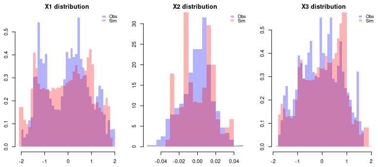
Figure B1 Distribution of reconstructed state variables at Torrey Pines. Histograms compare the distributions of the reconstructed variables X₁, X₂, and X₃ obtained from observations (blue) and from the simulated model trajectories (red).

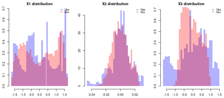
Figure B2 Distribution of reconstructed state variables at Gold Coast. Histograms compare the distributions of the reconstructed variables X₁, X₂, and X₃ obtained from observations (blue) and from the simulated model trajectories (red).

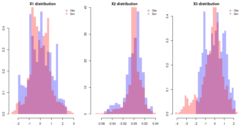
Figure B3 Distribution of reconstructed state variables at Ensenada. Histograms compare the distributions of the reconstructed variables X₁, X₂, and X₃ obtained from observations (blue) and from the simulated model trajectories (red).

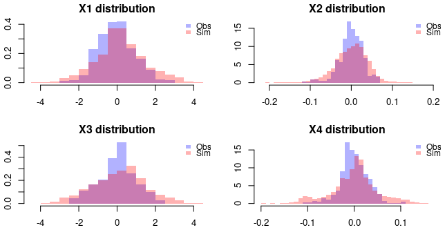
Figure B4 Distribution of reconstructed state variables at Duck. Histograms compare the distributions of the reconstructed variables X₁, X₂, X₃ and X₄ obtained from observations (blue) and from the simulated model trajectories (red).

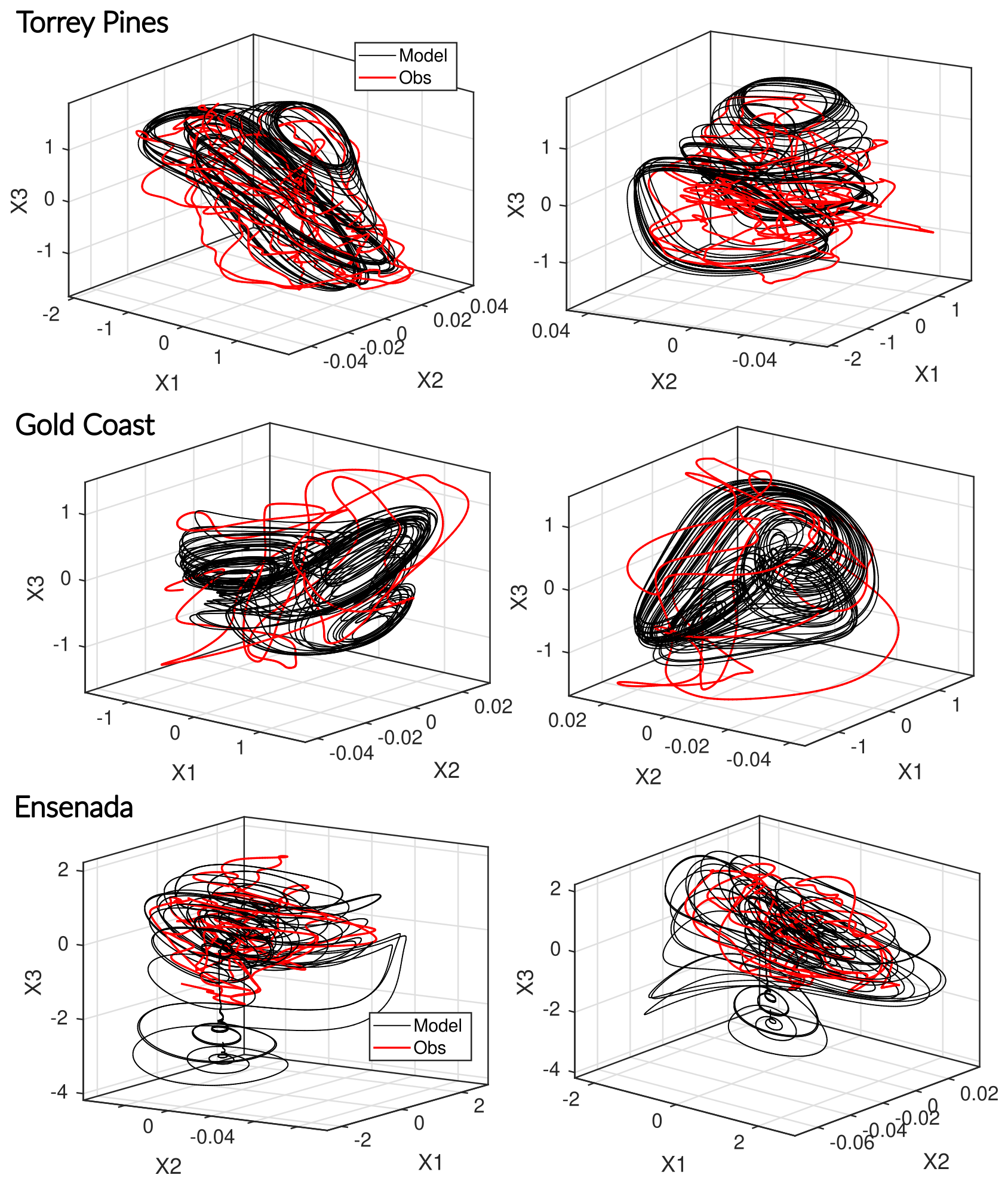
Figure B5 3D views of phase portraits for both the model and the observations, shown overlapping. Sites: Torrey Pines, Gold Coast, Ensenada.

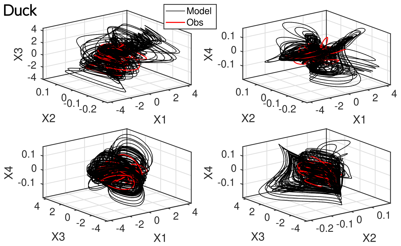
Figure B6 3D views of phase portraits for both the model and the observations, shown overlapping. Site: Duck

Table B1 First 4 statistical moments (mean, variance, skewness, kurtosis) for observations and model simulations at Torrey Pines, Gold Coast, Ensenada, and Duck.

Appendix C: Models' predictability horizon

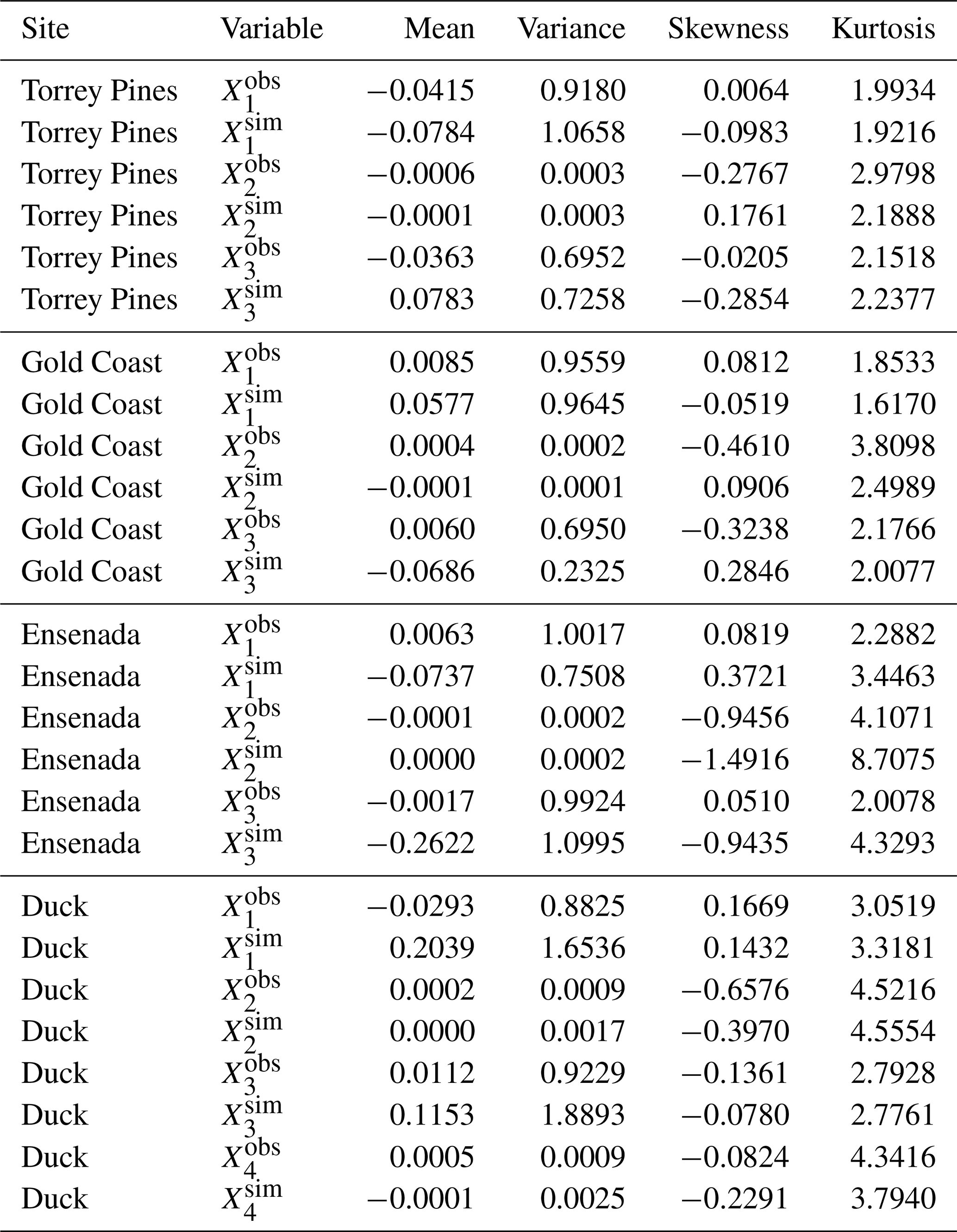
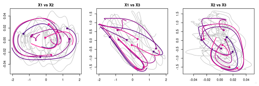
Figure C1 Torrey Pines. Ten simulations were integrated over 200 d from initial conditions randomly selected on the observations' phase portrait and subsequently perturbed by 2 % of the phase portrait standard deviation (dots).

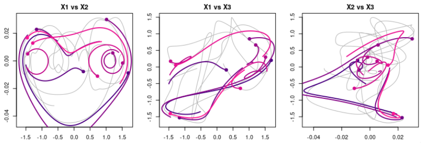
Figure C2 Gold Coast. Ten simulations were integrated over 200 d from initial conditions randomly selected on the observations' phase portrait and subsequently perturbed by 2 % of the phase portrait standard deviation (dots).

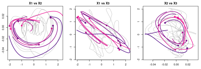
Figure C3 Ensenada. Ten simulations were integrated over 200 d from initial conditions randomly selected on the observations' phase portrait and subsequently perturbed by 2 % of the phase portrait standard deviation (dots).

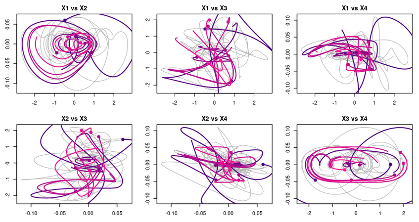
Figure C4 Duck. Ten simulations were integrated over 200 d from initial conditions randomly selected on the observations' phase portrait and subsequently perturbed by 2 % of the phase portrait standard deviation (dots).