Assessing Lagrangian coherence in atmospheric blocking

Atmospheric blocking exerts a major influence on mid-latitude atmospheric circulation and is known to be associated with extreme weather events. Previous work has highlighted the importance of the origin of air parcels that define the blocking region, especially with respect to non-adiabatic processes such as latent heating. So far, an objective method of clustering the individual Lagrangian trajectories passing through a blocking into larger and, more importantly, spatially coherent air streams has not been established. This is the focus of our study.

To this end, we determine coherent sets of trajectories, which are regions in the phase space of dynamical systems that keep their geometric integrity in time and can be characterized by robustness under small random perturbations. We approximate a dynamic diffusion operator on the available Lagrangian data and use it to cluster the trajectories into coherent sets. Our implementation adapts the existing methodology to the non-Euclidean geometry of Earth's atmosphere and its challenging scaling properties. The framework also allows for statements about the spatial behavior of the trajectories as a whole. We discuss two case studies differing with respect to season and geographic location.

The results confirm the existence of spatially coherent feeder air streams differing with respect to their dynamical properties and, more specifically, their latent heating contribution. Air streams experiencing a considerable amount of latent heating (warm conveyor belts) occur mainly during the maturing phase of the blocking and contribute to its stability. In our example cases, trajectories also exhibit an altered evolution of general coherence when passing through the blocking region, which is in line with the common understanding of blocking as a region of low dispersion.

1 Introduction

Atmospheric blocking represents a critical phenomenon in the dynamics of Earth's atmosphere, characterized by the temporary obstruction of prevailing westerlies in the mid-latitudes, potentially influencing weather on a planetary scale (Lupo, 2021). These events are notable for their role in causing extreme weather conditions, such as heat waves, cold spells and sustained periods of precipitation, impacting both human activities and natural ecosystems (Kautz et al., 2022; Pfahl and Wernli, 2012). The mechanisms leading to atmospheric blocking are complex, involving interactions between the atmosphere, cryosphere (Tyrlis et al., 2019; Woollings et al., 2014), ocean (Drijfhout et al., 2013; Häkkinen et al., 2011) and land (He et al., 2014; Kurgansky, 2020; Tilly et al., 2008) and are a subject of ongoing research. Despite their significance, predicting atmospheric blocking events and their impacts remains a challenge, due to the inherent variability and the multifaceted processes that govern their formation, maintenance and dissipation. Weather and climate models' inability to correctly represent blocking (Matsueda, 2009) also causes considerable uncertainties in its predicted response to climate change (Woollings et al., 2018).

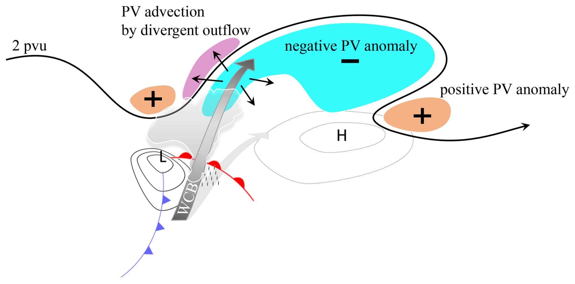
Though traditionally conceived as an adiabatic phenomenon, recent studies have pointed to the role of diabatic processes in blockings (Croci-Maspoli and Davies, 2009; Hauser et al., 2023; Pfahl et al., 2015; Tilly et al., 2008). More specifically, a line of study has been concerned with moist processes, arguing that a considerable fraction of the air masses constituting the blocking originate from warm sectors of neighboring surface cyclones and travel into the blocking via warm conveyor belts (WCBs) (Pfahl et al., 2015; Steinfeld and Pfahl, 2019; Yamamoto et al., 2021; Zschenderlein et al., 2020). WCBs are moist, rapidly ascending air streams and are subject to research in their own right (e.g.,  Joos et al., 2023; Madonna et al., 2014), among other things due to their contribution to forecast uncertainty (Madonna et al., 2015; Pickl et al., 2023; Wandel et al., 2021). According to Steinfeld and Pfahl (2019), the air parcels conveyed by such WCBs considerably influence the blocking by stabilizing and potentially intensifying the negative potential vorticity (PV) anomaly characteristic for the blocking, especially in the onset and maintenance stages of its life cycle (negative PV anomalies are associated with anticyclonal circulation and thus high pressure). This happens, firstly, through a material change in PV of the respective air masses via latent heating induced, cross-isentropic vertical motion and, secondly, through the divergent outflow of the guiding air streams in the upper troposphere. Evidence that moist processes might become more important in a warmer and moister climate underlines the need for further investigation (Steinfeld et al., 2022). A schematic depicting the procedural connections is reproduced from Steinfeld (2019) in Fig. 1.

Figure 1 Schematic showing a WCB air stream stabilizing a high pressure blocking, which is depicted as an upper-level negative potential vorticity (PV) anomaly. The line with 2 pvu (potential vorticity units) indicates the tropopause. Reproduced from Steinfeld (2019) with permission.

The notion of a WCB suggests a geometrically coherent flow of the air masses involved, but such a coherent behavior has not been explicitly addressed in the studies above. The backward trajectories attributed to such air streams are typically identified using thresholds for ascent (change in pressure) or diabatic heating (change in potential temperature) such that a common pathway is not guaranteed. In addition, the methodology employed does not allow for statements about the size, location, time of existence or even the number of WCBs implicated in the process. Another drawback of the identification method is its subjective nature implied by selecting an arbitrary threshold for the decrease in pressure (Madonna et al., 2014, use 600 hPa in 48 h) or increase in potential temperature the air parcels have experienced (usually a threshold of Δθ>2 K is used). To the best of our knowledge, an objective identification method for coherent medium- to large-scale air streams that allows these drawbacks to be addressed has not been presented in the context of atmospheric sciences.

In this study, we want to tackle these issues focusing on the exact spatio-temporal nature of trajectories passing through a blocking and how individual trajectories align with each other. By grouping the set of trajectories into subsets (clusters) based on only their geometric coherence, we identify synoptic-scale air streams and analyze their individual dynamical properties and interrelation with the large-scale flow configuration. The perspective introduced also allows for statements about the overall spatial configuration and coherence of the air parcels traced, especially with respect to the blockings' life cycles. A blocking's stabilizing and dispersion-suppressing nature affects individual air parcels, which can be identified through our Lagrangian lens (Ehstand et al., 2021).

To accomplish the above, we make use of the mathematical concept of coherent sets. A coherent set is a time-evolving region in the state space of a dynamical system that keeps its geometric integrity to a large degree. This is particularly interesting when the underlying system is such that individual trajectories diverge and any set eventually becomes highly filamented under evolution through the dynamics. We characterize coherent sets based on their stability under small perturbations. Coherent sets hence resist dispersion, persist longer in complicated flows and have thus an outstanding effect on the transport of physically relevant quantities. The fundamental idea is that in a coherent set the individual trajectories stay relatively close together as a whole, such that particles remain within the coherent set when they are subjected to small random perturbations. In contrast, if a time-evolving set is filamented, particles are likely to leave the set under the influence of random noise – and hence mix with its exterior. To formalize this heuristic and numerically compute coherent sets, we follow the work of Banisch and Koltai (2017) (based on theory developed in Froyland, 2013, 2015), which characterizes the robustness of coherent sets under small perturbations using a data-analysis framework called diffusion maps. Their method yields a single time-averaged operator whose spectral properties contain the necessary information to extract coherent sets.

The visual idea of coherence (i.e., “trajectories staying together”) can be cast into diverse objectives, which can then be used to partition available trajectory data into such sets. For a sample of the ideas that have been implemented, please consult Froyland and Padberg-Gehle (2015), Allshouse and Peacock (2015), Hadjighasem et al. (2016), Schlueter-Kuck and Dabiri (2017), Padberg-Gehle and Schneide (2017), and Koltai and Renger (2018). A related notion is that of Lagrangian coherent structures (Haller and Beron-Vera, 2013; Haller, 2015), aiming to describe barriers of transport. For their computation from finite trajectory data, see for instance Mowlavi et al. (2022).

The main foci of this study are the adaptation of the methodological framework of Banisch and Koltai (2017) to real-world trajectory data of air parcels in the atmosphere and its deployment for case studies of atmospheric blockings. This is motivated by the question of spatial coherence in WCBs in the context of blocking. As such, the presented work does not endeavor to give a one-size-fits-all solution to the problem of finding coherent air streams regardless of scale, geographic location and synoptic condition but should rather be understood as a proof of concept. We think atmospheric blocking is a phenomenon well suited for the application of the developed methodology, since it is large enough to feature a handful of distinct, coherent air streams (given the resolution of our data) but small enough to be well resolved by the number of trajectories computationally feasible. We have thoroughly analyzed two cases of atmospheric blocking differing with respect to both geographical location and time of year and show that differences between the two examples at similar points in their life cycles are notably smaller than differences within the same example between different points in the life cycles. This goes for the occurrence of WCBs, the overall trajectory density and the traced air masses' filamentation.

The paper is organized as follows. Section 2 introduces the mathematical foundation relevant to the methods employed. Section 3 covers details about the implementation of our algorithm as well as the data used. We show results from the application of the algorithm to test cases in Sect. 4 to both elucidate the concepts and methods introduced before and investigate the problems and questions posed above. Finally, Sect. 5 summarizes the findings.

2 Theory

To extract coherent sets from Lagrangian trajectory data, we employ the method proposed by Banisch and Koltai (2017). It uses local distances between data points to construct a diffusion operator that is used to estimate coherent sets by performing spectral clustering. In the following, we give a brief introduction into coherent sets and diffusion maps. Our aim is to provide a good intuitive understanding. For a formal and mathematically rigorous introduction of coherent sets using a transfer-operator-based framework, we refer to Banisch and Koltai (2017) and Froyland (2013). A thorough introduction to diffusion maps is given by Coifman and Lafon (2006).

2.1 Coherent sets

Informally put, coherent sets are time-dependent regions in space that remain largely intact as the system evolves. They exhibit a “natural” separation from their surrounding in the sense that flow across the boundary is small and geometric integrity is kept to a large degree. We characterize the geometric integrity of coherent sets by their robustness with respect to the addition of small noise. We first introduce the heuristics of coherent sets in an abstract setting before proceeding to the computation of coherent sets from trajectory data.

Consider the evolution of points over a finite number of time steps in a non-autonomous dynamical system. Let 𝕏_t⊂ℝⁿ be bounded sets which denote the domain of the dynamical system at each point in time. Here, t ranges over the integers from 0 to T. A non-autonomous dynamical system in discrete time over these time-evolving domains is given by a sequence of bijective maps ${\mathrm{\Phi }}_{t+\mathrm{1},t}:{\mathbb{X}}_t\to {\mathbb{X}}_{t+\mathrm{1}}$, where $\mathrm{0}\le t\le T-\mathrm{1}$. Before characterizing coherent sets of the dynamical system over the entire time frame from 0 to T, we study sets that are coherent under a single step.

Consider a bijective map $\mathrm{\Phi }:\mathbb{X}\to \mathbb{Y}$, with bounded domains $\mathbb{X},\mathbb{Y}\subset {\mathbb{R}}^n$. We say that a set 𝔸⊂𝕏 is coherent under Φ if the relation $({\mathrm{\Phi }}^{-\mathrm{1}}\circ \mathrm{\Phi })\left(\mathbb{A}\right)=\mathbb{A}$ is robust under the addition of small noise at both initial and final time. As a consequence, we require that the sets 𝔸 and Φ(𝔸) are not too filamented, i.e., that they possess high geometric integrity. Let 𝒟_ϵ be a diffusion operator that applies an ϵ-small random perturbation to any given point. The domain which 𝒟_ϵ acts on will be clear from the context, i.e., ${\mathcal{D}}_{\mathit{ϵ}}:\mathbb{X}\to \mathbb{X}$ or ${\mathcal{D}}_{\mathit{ϵ}}:\mathbb{Y}\to \mathbb{Y}$. A coherent set 𝔸⊂𝕏 of the map Φ has to satisfy 𝒟_ϵ𝔸≈𝔸 as well as $({\mathrm{\Phi }}^{-\mathrm{1}}\circ {\mathcal{D}}_{\mathit{ϵ}}\circ \mathrm{\Phi })\left(\mathbb{A}\right)\approx \mathbb{A}$. This heuristic is formulated more precisely in the language of transfer operators in Banisch and Koltai (2017).

The above heuristics describe coherent sets of a single map Φ. We return to the setting of a non-autonomous system over T time steps given by the maps ${\mathrm{\Phi }}_{t+\mathrm{1},t}$. A coherent set is a family of sets $({\mathbb{A}}_t{)}_{\mathrm{0}\le t\le T}$, where 𝔸_t⊂𝕏_t and ${\mathrm{\Phi }}_{t+\mathrm{1},t}\left({\mathbb{A}}_t\right)={\mathbb{A}}_{t+\mathrm{1}}$. Define the maps ${\mathrm{\Phi }}_{t,\mathrm{0}}={\mathrm{\Phi }}_{t,t-\mathrm{1}}\circ \mathrm{\dots }\circ {\mathrm{\Phi }}_{\mathrm{1},\mathrm{0}}$. For t=0, the map Φ_0,0 is simply the identity. A coherent set is completely characterized by 𝔸₀, in the sense that ${\mathbb{A}}_t={\mathrm{\Phi }}_{t,\mathrm{0}}\left({\mathbb{A}}_{\mathrm{0}}\right)$. We say that the family $({\mathbb{A}}_t{)}_{\mathrm{0}\le t\le T}$ is coherent if

$$\begin{array}{}\text{(1)}& ({\mathrm{\Phi }}_{t,\mathrm{0}}^{-\mathrm{1}}\circ {\mathcal{D}}_{\mathit{ϵ}}\circ {\mathrm{\Phi }}_{t,\mathrm{0}})\left({\mathbb{A}}_{\mathrm{0}}\right)\approx {\mathbb{A}}_{\mathrm{0}}\end{array}$$

for all t from 0 to T. We remark that this concept can be generalized to continuous time systems, e.g., Matthes et al. (2016).

Note that we assumed that 𝒟_ϵ maps from 𝕏_t into 𝕏_t; i.e., the random perturbation cannot map points outside of the domain 𝕏_t. This corresponds to, e.g., reflecting boundary conditions. For the purposes of our application, reflecting boundary conditions are physically not justifiable, since there are no physical boundaries for particles to be reflected at. Instead, we assume that 𝒟_ϵ can transport points outside of 𝕏_t. Since we assume no information about the dynamics outside of 𝕏_t, we consider points that are mapped outside of 𝕏_t as lost and hence unable to contribute to coherence. This corresponds to absorbing boundary conditions. We discuss how absorbing boundary conditions are implemented in the next subsection.

2.2 Diffusion maps

In the following, we give a brief introduction to diffusion maps. A mathematically rigorous derivation can be found in Coifman and Lafon (2006) and Ghojogh et al. (2022).

Assume the data of m trajectories of a non-autonomous dynamics are provided in the form of data points $x_t^i\in {\mathbb{R}}^n$, where $\mathrm{1}\le i\le m$ and t ranges over the integers from 0 to T. We assume that in each time frame the point cloud $X_t=\mathit{\left\{}{x}_t^i\right|\mathrm{1}\le i\le m\mathit{\}}$ approximates a bounded manifold 𝕏_t⊂ℝⁿ and that the data points are sample trajectories of a – potentially unknown – non-autonomous dynamics ${\mathrm{\Phi }}_{t+\mathrm{1},t}:{\mathbb{X}}_t\to {\mathbb{X}}_{t+\mathrm{1}}$, i.e., ${\mathrm{\Phi }}_{t,s}\left(x_s^i\right)=x_t^i$ for all s≤t. Our goal is to characterize coherent sets of this dynamics, in particular to formalize the heuristic in Eq. (1) in the setting of discrete trajectory data. A coherent set consists of a certain subset of the point cloud, i.e., $A_t:=\mathit{\left\{}{x}_t^i\right|i\in \mathcal{I}\mathit{\}}\subset X_t$, where $\mathcal{I}\subset \mathit{\{}\mathrm{1},\mathrm{\dots },m\mathit{\}}$ is a set of indices. In order to formalize the heuristic in Eq. (1), we introduce a discretization of the operator ${\mathcal{D}}_{\mathit{ϵ}}:{\mathbb{X}}_t\to {\mathbb{X}}_t$ acting on the point cloud X_t.

Since X_t is a finite set of size m, we construct a transition probability matrix ${\widehat{\mathbf{P}}}_{t,\mathit{ϵ}}\in {\mathbb{R}}^{m\times m}$ that simulates diffusion on X_t of strength ϵ. The rest of this section is devoted to constructing the matrix ${\widehat{\mathbf{P}}}_{t,\mathit{ϵ}}$ for each $\mathrm{0}\le t\le T$, as well as discussing the implementation of boundary conditions. We remark that we do not need to approximate the dynamics ${\mathrm{\Phi }}_{t+\mathrm{1},t}$ to use Eq. (1), since we assume to have the data already in the form of trajectories.

Let k_ϵ be a symmetric diffusion kernel with scale parameter ϵ. This kernel encodes the proximity of two data points; i.e., k_ϵ(xⁱ,x^j) is large if xⁱ and x^j are close and small if the points are far apart. In the following, we use the Gaussian kernel for an arbitrary metric $\text{dist}(\cdot ,\cdot )$ on ℝⁿ,

$$\begin{array}{}\text{(2)}& k_{\mathit{ϵ}}(x^i,x^j)=\exp \left(-{\displaystyle \frac{\text{dist}(x^i,x^j{)}^{\mathrm{2}}}{\mathit{ϵ}}}\right).\end{array}$$

In general, it is natural to use the Euclidean distance $\text{dist}(x^i,x^j)=\Vert x^i-x^j\Vert$. However, for the application to atmospheric data, which is a non-isotropic setting, we are going to use an alternative distance aiming to establish isotropy with respect to turbulent diffusion; see Sect. 3.4. For each time step $\mathrm{0}\le t\le T$, we construct the similarity matrix ${\mathbf{K}}_{t,\mathit{ϵ}}\in {\mathbb{R}}^{m\times m}$,

$$\begin{array}{}\text{(3)}& {\left[{\mathbf{K}}_{t,\mathit{ϵ}}\right]}_{i,j}=k_{\mathit{ϵ}}(x_t^i,x_t^j).\end{array}$$

Note that K_t,ϵ is symmetric, and all diagonal entries are 1, while all off-diagonal entries are between 0 and 1. In practice, a cutoff radius is used to increase the sparsity of the matrix by setting entries ${\left[{\mathbf{K}}_{t,\mathit{ϵ}}\right]}_{i,j}$ that are below a specified threshold to 0. Since the value ${\left[{\mathbf{K}}_{t,\mathit{ϵ}}\right]}_{i,j}$ decays monotonically in the distance between $x_t^i$ and $x_t^j$, we may equivalently choose a cutoff radius r and set ${\left[{\mathbf{K}}_{t,\mathit{ϵ}}\right]}_{i,j}$ to 0 if $\text{dist}(x_t^i,x_t^j)>r$. Here, we choose $r=\mathrm{3}\sqrt{\mathit{ϵ}}$, which is an appropriate scaling for a Gaussian kernel k_ϵ.

To account for differences in the density of the point cloud, we pre-normalize the similarity matrix:

$$\begin{array}{}\text{(4)}& {\left[{\mathit{u}}_{t,\mathit{ϵ}}\right]}_i:=\sum _{j=\mathrm{1}}^m{\left[{\mathbf{K}}_{t,\mathit{ϵ}}\right]}_{i,j},{\left[{\widehat{\mathbf{K}}}_{t,\mathit{ϵ}}\right]}_{i,j}:={\displaystyle \frac{{\left[{\mathbf{K}}_{t,\mathit{ϵ}}\right]}_{i,j}}{{\left[{\mathit{u}}_{t,\mathit{ϵ}}\right]}_i{\left[{\mathit{u}}_{t,\mathit{ϵ}}\right]}_j}}.\end{array}$$

Finally, the diffusion matrix ${\widehat{\mathbf{P}}}_{\mathit{ϵ}}$ is obtained by row normalization:

$$\begin{array}{}\text{(5)}& {\left[{\mathit{v}}_{t,\mathit{ϵ}}\right]}_i:=\sum _{j=\mathrm{1}}^m{\left[{\widehat{\mathbf{K}}}_{t,\mathit{ϵ}}\right]}_{i,j},{\left[{\widehat{\mathbf{P}}}_{t,\mathit{ϵ}}\right]}_{i,j}:={\displaystyle \frac{{\left[{\widehat{\mathbf{K}}}_{t,\mathit{ϵ}}\right]}_{i,j}}{{\left[{\mathit{v}}_{t,\mathit{ϵ}}\right]}_i}}.\end{array}$$

The matrix ${\widehat{\mathbf{P}}}_{t,\mathit{ϵ}}$ is non-negative and normalized such that it is row-stochastic (often called left-stochastic); i.e., the entries of each row sum to 1. Hence, ${\widehat{\mathbf{P}}}_{t,\mathit{ϵ}}$ can be understood as transition probabilities on the point cloud $\mathit{\left\{}{x}_t^i\right|\mathrm{1}\le i\le m\mathit{\}}$ that simulate a discretized diffusion on the point cloud X_t. In the data-rich limit, ${\widehat{\mathbf{P}}}_{t,\mathit{ϵ}}$ is a self-adjoint operator, i.e., a symmetric matrix.

Lastly, we address the implementation of boundary conditions. Since ${\widehat{\mathbf{P}}}_{t,\mathit{ϵ}}$, as constructed above, is a stochastic matrix, all points in X_t remain in X_t; i.e., there are reflecting boundary conditions. However, in the context of atmospheric flow of air masses, where 𝕏_t is a bounded, time-dependent region of the atmosphere, it is unnatural to assume turbulent diffusion would not act across the boundaries of 𝕏_t. Since we assume no information about the dynamics outside of 𝕏_t, we assume absorbing boundary conditions; i.e., all points on the boundary of X_t are removed. Hence, we need to determine a set of boundary points $\partial X_t\subset X_t$. Determining these point algorithmically is the content of Sect. 2.6. Given a set of boundary points ∂X_t, we integrate absorbing boundary conditions into the transition matrix ${\widehat{\mathbf{P}}}_{t,\mathit{ϵ}}$ by removing the rows and columns corresponding to the boundary points. In order to keep the dimensions of the matrices compatible across different time steps, we implement this by setting the respective rows and columns to 0 instead of removing them:

$$\begin{array}{}\text{(6)}& {\left[{\mathbf{P}}_{t,\mathit{ϵ}}\right]}_{i,j}:=\left\{\begin{array}{l}\mathrm{0},x_t^i\in \partial X_t,\text{ or }{x}_t^j\in \partial X_t,\\ {\left[{\widehat{\mathbf{P}}}_{t,\mathit{ϵ}}\right]}_{i,j},\text{else}.\end{array}\right.\end{array}$$

By construction, P_t,ϵ is a substochastic matrix. In summary, ${\widehat{\mathbf{P}}}_{t,\mathit{ϵ}}$ corresponds to a discretized diffusion matrix with reflecting boundary conditions, while P_t,ϵ corresponds to a discretized diffusion matrix with absorbing boundary conditions. For the purposes of our application, we will go forward using the substochastic matrix P_t,ϵ.

2.3 Spectral clustering

Having constructed the diffusion matrices P_t,ϵ, we describe how to compute coherent sets using a spectral clustering method. A coherent set A_t, where $\mathrm{0}\le t\le T$, is given by $A_t=\mathit{\left\{}{x}_t^i\right|i\in \mathcal{I}\mathit{\}}$, where $\mathcal{I}\subset \mathit{\{}\mathrm{1},\mathrm{\dots },m\mathit{\}}$ is a set of indices. In particular, we find ${\mathrm{\Phi }}_{t,\mathrm{0}}{A}_{\mathrm{0}}=A_t$. Hence, the heuristic in Eq. (1), using the diffusion matrix P_t,ϵ introduced in the previous section, requires that indices i∈ℐ have a high transition probability to ℐ, i.e.,

$${\left[{\mathbf{P}}_{t,\mathit{ϵ}}\right]}_{i,\mathcal{I}}:=\sum _{j\in \mathcal{I}}{\left[{\mathbf{P}}_{t,\mathit{ϵ}}\right]}_{i,j}\approx \mathrm{1}.$$

for all i∈ℐ. This approximation should be as accurate as possible for all $\mathrm{0}\le t\le T$. We construct the averaged diffusion operator

$$\begin{array}{}\text{(7)}& {\mathbf{Q}}_{\mathit{ϵ}}:={\displaystyle \frac{\mathrm{1}}{T+\mathrm{1}}}\sum _{t=\mathrm{0}}^T{\mathbf{P}}_{t,\mathit{ϵ}}.\end{array}$$

This averaged diffusion operator was introduced in Froyland (2015) and it was shown that coherent sets can be extracted from the dominant eigenvectors of Q_ϵ. Equation (7) should be understood as a quantitative version of averaging the left-hand side of Eq. (1). Thus, eigenvectors of Q_ϵ for eigenvalues close to 1 represent functional representations of sets that satisfy Eq. (1) on average for $\mathrm{0}\le t\le T$.

To better understand how coherent sets are related to the eigenvectors of Q_ϵ, assume that there are K idealized coherent sets $A_t^k$, for $\mathrm{1}\le k\le K$, corresponding to the sets of indices ℐ^k. These sets are idealized coherent sets in the sense that ${\left[{\mathbf{Q}}_{\mathit{ϵ}}\right]}_{i,\mathcal{I}}=\mathrm{1}$ for all i∈ℐ^k. Since Q_ϵ is substochastic, this implies that Q_ϵ has a block-diagonal structure with blocks indicated by the sets ℐ^k. In particular, for each $\mathrm{1}\le k\le K$, the matrix Q_ϵ has an eigenvector with eigenvalue 1 that is supported only on the set ℐ^k. Hence, the K coherent sets ℐ^k can be extracted from eigenvectors to the K largest eigenvalues. Additionally, there is an (K+1)th set, which is the complement of the union of the ℐ^k, which we call the residual set. The temporal evolution of 𝕏_t and, equivalently X_t, implies that ∂X_t is time-dependent as well, such that the residual set is not necessarily equal to ∂X_t. The residual set, together with the coherent sets ℐ^k, forms a partition of the set of all points $\mathit{\{}\mathrm{1},\mathrm{\dots },m\mathit{\}}$.

Returning to the general setting, we compute the eigenvalues of the matrix Q_ϵ. In the data-rich limit, the matrix Q_ϵ is symmetric and, thus, only has real eigenvalues. If complex eigenvalues occur numerically, we discard the imaginary part and only consider their real part. We order the eigenvalues from large to small. Since Q_ϵ is substochastic, all eigenvalues lie between 0 and 1. We say that there is a spectral gap after the Kth eigenvalue if the (K+1)st eigenvalue is significantly smaller than the first K eigenvalues. We call these first K eigenvalues the dominant spectrum and the corresponding eigenvectors the dominant eigenvectors. After identifying a spectral gap, we perform a k--means clustering of the set of points $\mathit{\{}\mathrm{1},\mathrm{\dots },m\mathit{\}}$ using the information of the dominant eigenvectors. Assuming that the dominant spectrum consists of K eigenvalues, each point in $\mathit{\{}\mathrm{1},\mathrm{\dots },m\mathit{\}}$ has K characteristic values, namely the entries of the K dominant eigenvectors. Using the k--means algorithm, we group the m points into K+1 clusters ℐ^k, for $\mathrm{1}\le k\le K+\mathrm{1}$. Motivated by the idealized setting, K of these sets corresponds to coherent sets, while there is an additional (K+1)th residual set. See Fig. 5 for an example of the spectrum of Q_ϵ as well as the spectral clustering of the point cloud. The residual set is colored in gray.

2.4 Quantifying coherence

To evaluate and interpret the computation of coherent sets in application, it is crucial to introduce a quantification of coherence of each of the clusters ℐ_k. Given a set of indices ${\mathcal{I}}_k\subset \mathit{\{}\mathrm{1},\mathrm{\dots },m\mathit{\}}$, we restrict the averaged diffusion matrix Q_ϵ to the indices ℐ_k and compute the sum of its entries, divided by the size of ℐ_k. Heuristically, this corresponds to the probability that a point that is randomly chosen from ℐ_k is mapped to another point in ℐ_k. As a notion of coherence we use the complementary probability, namely

$$\begin{array}{}\text{(8)}& P_{\text{exit}}\left({\mathcal{I}}_k\right)=\mathrm{1}-{\displaystyle \frac{\mathrm{1}}{\left|{\mathcal{I}}_k\right|}}\sum _{i,j\in {\mathcal{I}}_k}{\left[{\mathbf{Q}}_{\mathit{ϵ}}\right]}_{i,j}.\end{array}$$

Note that since Q_ϵ is substochastic, P_exit(ℐ_k) is between 0 and 1. A value close to 0 corresponds to high coherence because the trajectories are tightly bundled with respect to the averaged diffusion matrix Q_ϵ. By construction, the exit whose probability is quantified can be to another coherent set, to the residual set or out of the set of all trajectories (see the discussion of boundary conditions in Sect. 2.2).

In the idealized setting where ${\left[{\mathbf{Q}}_{\mathit{ϵ}}\right]}_{i,{\mathcal{I}}_k}=\mathrm{1}$ for all i∈ℐ_k, the restriction ${\left[{\mathbf{Q}}_{\mathit{ϵ}}\right]}_{{\mathcal{I}}_k,{\mathcal{I}}_k}$ is a stochastic matrix, and we find P_exit(ℐ_k)=0. For the spectral clustering method described in the previous subsection, we expect to obtain K sets with relatively high coherence and one residual set with a lower coherence. We verify this for two case studies in Sect. 4. For comparison, for each coherent or residual set found, we also calculate P_exit for 100 test sets and show their distribution as box-and-whisker plots. Each of these test sets is generated by picking a random trajectory and selecting the m closest points (with respect to the custom metric to be introduced in Sect. 3.4) in the initial distribution (t=0), where $m=\left|{\mathcal{I}}_k\right|$ is the number of points in the set to compare. Therefore, at t=0, the test sets resemble sets with minimal surfaces for a given volume (more specifically, intersections of balls with the initial distribution), which we consider a suitable basis for comparison.

Another option to quantify coherence is to compute the largest eigenvalue of the restricted matrix ${\left[{\mathbf{Q}}_{\mathit{ϵ}}\right]}_{{\mathcal{I}}_k,{\mathcal{I}}_k}$, which determines the complement of the exit probability defined above under the stationary distribution of the respective set instead of a uniform distribution. Since Q_ϵ is substochastic, the largest eigenvalue of the restricted matrix lies between 0 and 1, where a larger value corresponds to higher coherence. We provide this measure in the Supplement.

2.5 Choosing ϵ

Recall the definition of the similarity matrix ${\mathbf{K}}_{t,\mathit{ϵ}}\in {\mathbb{R}}^{m\times m}$ in Eq. (3) with the diffusion kernel introduced in Eq. (2), where $\text{dist}(\cdot ,\cdot )$ is a metric on ℝⁿ. Under the assumption that the points $x_t^i$ are distributed uniformly with respect to $\text{dist}(\cdot ,\cdot )$, it is argued in Appendix A.2 of Koltai and Weiss (2020) and following Berry and Harlim (2016) and Coifman et al. (2008) that ϵ>0 should be chosen, if possible, such that the following approximation is valid:

$$\begin{array}{}\text{(9)}& \begin{array}{rl}{\displaystyle }{S}_t\left(\mathit{ϵ}\right):=& {\displaystyle }\sum _{i,j}{\left[{\mathbf{K}}_{t,\mathit{ϵ}}\right]}_{i,j}\\ {\displaystyle }\approx & {\displaystyle }{\sum }_{i=\mathrm{1}}^{m}C\underset{{\mathbb{R}}^{d\left(t\right)}}{\int }\exp \left(-{\displaystyle \frac{\Vert x_t^i-y{\Vert }^{\mathrm{2}}}{\mathit{ϵ}}}\right)\mathrm{d}y\\ {\displaystyle }=& {\displaystyle }mC(\mathit{ϵ}\mathit{\pi }{)}^{d\left(t\right)/\mathrm{2}},\end{array}\end{array}$$

where C>0 is a constant that depends on how densely the points in X_t populate 𝕏_t, and d(t) is the dimension of the manifold 𝕏_t. To better understand the constants C and d(t), assume that X_t is a large d-dimensional grid of grid length ℓ and consider the Euclidean distance $\text{dist}(x,y)=\Vert x-y\Vert$. Then, the sum S_t(ϵ) corresponds to a Riemannian integral approximation, and the approximation in Eq. (9) is valid, with C being the average number of points per unit of volume, which is given by $C\approx {\mathrm{\ell }}^{-d}$, i.e., $\mathrm{\ell }=C^{-\mathrm{1}/d}$.

Taking the logarithm on both sides of Eq. (9) reveals an affine linear connection between log (S_t(ϵ)) and log (ϵ):

$$\begin{array}{}\text{(10)}& \log \left(S_t\right(\mathit{ϵ}\left)\right)\approx {\displaystyle \frac{d\left(t\right)}{\mathrm{2}}}\log \left(\mathit{ϵ}\right)+\log \left(C\right)+\log \left(m\right)+{\displaystyle \frac{d\left(t\right)}{\mathrm{2}}}\log \left(\mathit{\pi }\right).\end{array}$$

Hence, in order to determine a range of suitable values for ϵ, we plot the function S_t(ϵ) versus ϵ in a log–log plot for each time t and look for a range of ϵ in which the graph is linear. See Fig. 3 for an example. Additionally, we can read off the dimension d(t), as well as a measure of density $\mathrm{\ell }\left(t\right)=C^{-\mathrm{1}/d\left(t\right)}$ of the point cloud X_t.

$$\begin{array}{}\text{(11)}& {\displaystyle }d\left(t\right):=\mathrm{2}\cdot \begin{array}{c}\max \\ \mathit{ϵ}>\mathrm{0}\end{array}{\displaystyle \frac{\partial \log \left(S_t\right(\mathit{ϵ}\left)\right)}{\partial \log \left(\mathit{ϵ}\right)}}\text{(12)}& {\displaystyle }\mathrm{\ell }\left(t\right):=C^{-\mathrm{1}/d\left(t\right)}={\left({\displaystyle \frac{S_t{\mathit{ϵ}}^{*}}{m}}\right)}^{\mathrm{1}/d\left(t\right)}({\mathit{ϵ}}^{*}\mathit{\pi }{)}^{\mathrm{1}/\mathrm{2}},\end{array}$$

where ${\mathit{ϵ}}^{*}>\mathrm{0}$ is the value that maximizes the slope $\partial \log \left(S_t\right(\mathit{ϵ}\left)\right)/\partial \log \left(\mathit{ϵ}\right)$. We note that the derivations of d(t) and ℓ(t) are not mathematically rigorous and are used heuristically. In particular, the dimension d(t) does not have to be an integer, and ℓ(t) is just an approximate measure of (inverse) density when the point cloud X_t is not a perfect grid. We stress that since ℓ(t) approximates a grid length, higher values correspond to lower point densities. In addition, we note that d(t) is invariant under isotropic contraction/expansion of X_t (it is scale-invariant), but ℓ(t) is not.

2.6 Boundary handling with α shapes

The estimation of coherent sets requires proper handling of boundary points $\partial X_t\subset X_t$. Hence, a method is needed to determine which points lie on the boundary of a given point cloud X_t. This problem reduces to the well-researched problem of surface reconstruction from point cloud data. The simplest approach is to use the uniquely defined convex hull of X_t. This method is too coarse for our purpose, since the point cloud X_t is in general not a convex object. Once concavity is permitted, detection of a bounding surface of a set of points is ambiguous, and several algorithmic approaches exist (Berger et al., 2017). We have decided on using the established alpha shape algorithm first introduced by Edelsbrunner et al. (1983) (see Edelsbrunner, 2011, for an overview), since it does not require surface normals and can be conveniently tuned by only one parameter α≥0. Large values of α correspond to a structured surface, while small values of α result in a smooth surface. For a thorough derivation and details on algorithmic implementation, consult Edelsbrunner and Mücke (1994).

Let X_t⊂ℝⁿ be a finite set of points, $\mathrm{0}\le \mathit{\alpha }<\mathrm{\infty }$, a real number. We denote open balls in ℝⁿ of radius α by b_α. An α ball b_α is said to be empty if it does not contain any points from X_t. The α hull ℍ_α is then defined as the complement of the union of all empty α balls:

$$\begin{array}{}\text{(13)}& {\mathbb{H}}_{\mathit{\alpha }}:={\mathbb{R}}^n\backslash \bigcup _{b_{\mathit{\alpha }}\cap X_t=\mathrm{\varnothing }}{b}_{\mathit{\alpha }}.\end{array}$$

We define the boundary of X_t to consist of those points that lie in the boundary of ℍ_α, i.e.,

$$\partial X_t:=\mathit{\{}x\in X_t|x\in \partial {\mathbb{H}}_{\mathit{\alpha }}\mathit{\}}.$$

An equivalent definition of the boundary is that x∈X_t lies in ∂X_t if and only if there is an empty open α ball b_α such that $x\in \partial b_{\mathit{\alpha }}$. As α→∞ the set ℍ_α recovers the convex hull, whereas α=0 results in ℍ_α=X_t. Hence, the set ∂X_t grows as α→0, and for α small enough, we find $\partial X_t=X_t$.

This sparks the question of choosing α appropriately such that ∂X_t defines a boundary of the point cloud X_t of the desired coarseness. As discussed in Sect. 2.5, $\sqrt{{\mathit{ϵ}}^{*}}$ provides a measure of the typical distance between points in the point cloud. Therefore, it is natural to choose α in the same magnitude as $\sqrt{{\mathit{ϵ}}^{*}}$.

The alpha shape algorithm assumes the points live in Euclidean space. However, in Sect. 4 we apply our methods to atmospheric data. The atmosphere, being approximated by a spherical shell, is non-isotropic and globally non-Euclidean. Thus, constructing a hull in a Cartesian coordinate system, e.g., centered in Earth's core, is destined to fail as the large difference in scales between vertical and horizontal coordinates leads to points being sampled from a nearly two-dimensional region in space. In such a perspective, virtually all points would be boundary points. We have therefore decided to apply a stereographic projection centered at the North Pole with an undistorted latitude of 50° N to the horizontal coordinates and applied a linear vertical scaling in accordance with the custom distance metric introduced in Sect. 3.4 before applying the alpha shape algorithm. A stereographic projection seems apt since the air parcels of our examples stay in the Northern Hemisphere and are gathered around the mid-latitudes for most of the time. Other suitable coordinate transformations alter the selected boundary points only to a small degree and do not change the resulting coherent sets detected significantly (not shown).

3 Implementation

All atmospheric fields used in the analysis are taken from the ERA5 reanalysis product provided by the European Centre for Medium-Range Weather Forecasts (ECMWF) (Hersbach et al., 2020). It resolves the global atmosphere on a grid with a roughly 31 km horizontal spacing and 137 hybrid vertical levels between the surface and 1 hPa on an hourly timescale.

3.1 Blocking identification

The atmospheric blocking regions are defined as in Pfahl and Wernli (2012)  who utilized the algorithm introduced by Schwierz et al. (2004). More specifically, grid points are identified as blocked if a vertically averaged (between 500 and 150 hPa; the upper troposphere) negative PV anomaly (with respect to the monthly climatology) larger than 1.3 pvu (10⁻⁶ K m² kg⁻¹ s⁻¹) for at least 5 d is observed for a potentially traveling connected region (individual grid points need not experience this anomaly for 5 full days). Data are available in 6-hourly time steps, and PV anomalies are required to have a spatial overlap of at least 70 % to be assigned to the same track.

Though a host of different blocking identification mechanisms are available (Pinheiro et al., 2019), this PV-based algorithm has been chosen since it encapsulates the most important dynamical features of atmospheric blocking (Schwierz et al., 2004; Croci-Maspoli et al., 2007) and directly identifies two-dimensional regions. The identified regions will usually mark the areas responsible dynamically for the blocking characteristics (i.e., the high-pressure ridge regions) rather than the areas marked by a geopotential height reversal. The focus of this study lies on the demonstration of the methodological framework when applied to atmospheric blocking air streams rather than in arriving at definitive or quantitative insights into blocking consistent across different blocking definitions, which is why we abstain from comparing results between different blocking indices.

3.2 Initial points

The method for the identification of coherent air streams described in Sect. 2 is applied to two case studies. Given the two-dimensional, global Boolean field of whether a grid point is blocked or not, for each case, an atmospheric blocking event is identified as a connected region of True values developing in time. For an individual time step, a respective region is “filled” with trajectory initial points with a vertical distance of 7 hPa between 550 and 150 hPa (we choose 550 hPa instead of 500 hPa for a slightly broader scope; the same does not apply for the upper limit, since it would likely cross the tropopause) and a horizontal distance given by the scale difference parameter κ times the vertical distance (see Sect. 3.4). In our case study, for a scaling parameter of κ=15 km hPa⁻¹, a horizontal distance of 105 km was used. Such a point density has emerged as the highest possible point density that still allowed for an acceptable computational complexity. A zero-mean Gaussian noise with standard deviation equal to a quarter of the distance in the respective direction is then added to each point individually to prevent the regular structure of the initial point distribution from biasing the coherent set clustering later on. Finally, all initial points that lie above the dynamic tropopause – defined as the 2 pvu isosurface – are removed.

3.3 Trajectory calculation

The initial points are then used to calculate 3 d forward and backward trajectories from three-dimensional wind fields on model levels using the LAGRangian ANalysis TOol (LAGRANTO) (Sprenger and Wernli, 2015), which employs an iterative predictor–corrector procedure. We think of the resulting trajectories as solutions of the dynamical system describing the motion of air parcels in the atmosphere ($x_t^i$ from Sect. 2). Various dynamical variables can be traced along the path of the air parcels' trajectories including potential temperature θ, specific humidity q, temperature T, and all coordinates and velocities. These will reveal the dynamical properties present in the clusters generated from purely geometric information.

3.4 Distance calculation

Our methodology presented in Sect. 2 is based on point-wise distance calculation. Here, again, the issue of vastly different length scales in the horizontal and vertical directions arises. Resorting to a map projection as with the alpha shapes algorithm described in Sect. 2.6 does, however, not seem to be the best option since errors introduced during the stereographic projection can be avoided. This is because calculating distances between points does not necessarily require the points to live in Euclidean space. In contrast to Banisch and Koltai (2017), who relied on the Euclidean norm as a measure of distance, we therefore construct a non-Euclidean distance which connects the vertical and horizontal scales through a scale parameter κ:

$$\begin{array}{}\text{(14)}& \mathit{\kappa }={\displaystyle \frac{\stackrel{\mathrm{‾}}{\sqrt{u^{\mathrm{2}}+v^{\mathrm{2}}}}}{\stackrel{\mathrm{‾}}{\mathrm{|}\mathit{\omega }\mathrm{|}}}}={\displaystyle \frac{{\sum }_{i=\mathrm{1}}^m{\sum }_{t=\mathrm{0}}^T\sqrt{(u_t^i{)}^{\mathrm{2}}+(v_t^i{)}^{\mathrm{2}}}}{{\sum }_{i=\mathrm{1}}^m{\sum }_{t=\mathrm{0}}^T\mathrm{|}{\mathit{\omega }}_t^i\mathrm{|}}},\end{array}$$

where $u_t^i$ and $v_t^i$ are the two horizontal and ${\mathit{\omega }}_t^i$ the vertical velocity component of the ith air parcel at time t. For two points $x^i=({\mathit{\phi }}^i,{\mathit{\lambda }}^i,p^i)$ and $x^j=({\mathit{\phi }}^j,{\mathit{\lambda }}^j,p^j)$, given by their respective latitudes φ, longitudes λ and pressure level p, we then define

$$\begin{array}{}\text{(15)}& {\displaystyle }\text{dist}(x^i,x^j)=\sqrt{{\text{dist}}_{\mathrm{h}}(x^i,x^j{)}^{\mathrm{2}}+(\mathit{\kappa }(p^j-p^i){)}^{\mathrm{2}}},\text{(16)}& {\displaystyle }\begin{array}{rl}& {\text{dist}}_{\mathrm{h}}(x^i,x^j)=\mathrm{2}{r}_{\mathrm{E}}\arcsin \\ & \left(\sqrt{{\sin }^{\mathrm{2}}\left({\displaystyle \frac{{\mathit{\phi }}^j-{\mathit{\phi }}^i}{\mathrm{2}}}\right)+\cos {\mathit{\phi }}^i\cdot \cos {\mathit{\phi }}^j\cdot {\sin }^{\mathrm{2}}\left({\displaystyle \frac{{\mathit{\lambda }}^j-{\mathit{\lambda }}^i}{\mathrm{2}}}\right)}\right),\end{array}\end{array}$$

where r_E stands for Earth's radius. The distance is symmetric and positive. The horizontal distance dist_h is the Haversine distance which approximates the great-circle distance of two points on Earth's surface (assuming a spherical shape) well (Green, 1977).

For the scale parameter κ, a heuristic approach has been chosen that estimates the difference in scales by comparing average horizontal and vertical velocities, where the average is taken over all trajectories and time steps. We think of distances as similar if air parcels take roughly the same amount of time to overcome them given some average velocity, which is the reasoning behind the construction of κ. In addition, atmospheric turbulence – the dominant source of diffusion at the scales investigated here – roughly scales with velocity. The developed notion of distance relies only on geometric information (if one conceives velocities as geometric), which allows comparison of purely geometric coherence to similarity of dynamic properties. For the construction of κ, we have deliberately abstained from including measures of vertical stability or asymptotic methods since the phenomena investigated feature relevant processes on the synoptic scale as well as the mesoscale, which would further complicate the choice of scale-connecting characteristic quantities (Klein, 2010). Note that, due to the definition of κ in Eq. (14), the custom metric $\text{dist}(\cdot ,\cdot )$ is formally measured in kilometers.

We remark that estimated values of κ varied only by roughly 20 %, and results were rather insensitive to the exact value of κ applied in both the algorithm and the initial point generation. For ease of computation and comparability between cases, we have therefore decided to choose a constant κ=15 km hPa⁻¹ across all cases investigated. Note that requiring exact equality between the empirical κ and the κ used in the initial point generation would require extensive iteration, since the empirical κ depends on the trajectories, which, in turn, depend on the initial point locations.

4 Case studies

4.1 Canada 2016

As a first example, the strong Ω blocking observed from late April to early May 2016 over Canada is investigated. It is considered one of the main causes of the 2016 Fort McMurray wildfire, the costliest disaster in Canadian history up to that date (Statistics Canada, 2017). The blocking identification data set introduced in Sect. 3 identifies blocked grid points from 29 April 2016 at 06:00 UTC to 5 May 2016 at 00:00 UTC. Synoptic conditions along with the blocking region are shown for three time steps representative of onset, maintenance and decay in Fig. 2. A video of synoptic conditions at all time steps is provided in the Supplement.

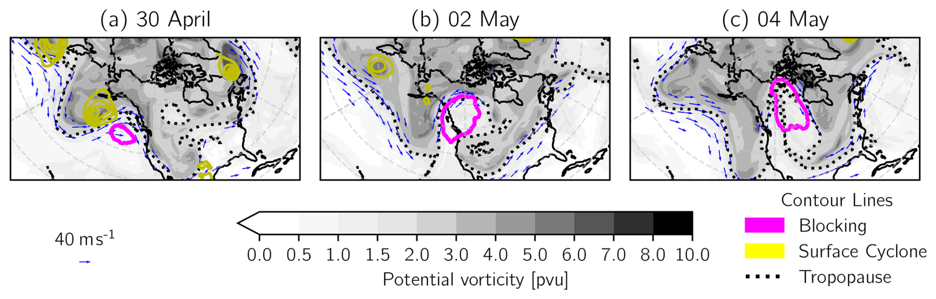
Figure 2 Synoptic conditions at three time instances (all at 00:00 UTC) during the 2016 Canada case. Upper-level PV (shaded), 2 pvu contour (tropopause) in black, upper-level wind (blue vectors, only shown for wind speeds larger than 30 m s⁻¹), surface cyclones (sea level pressure; yellow contours from 980 to 1000 hPa every 5 hPa) and blocking region (magenta contour; see Sect. 3.1 for definition). Upper-level fields are vertically averaged between 500 and 150 hPa. Note that horizontal wind velocity is indicated by the quivers' length. Denser quivers towards the poles result from denser longitudes.

During the onset phase (a), the co-located surface cyclone and upper-tropospheric trough just east of the dateline induced a poleward transport of warm, low-PV air masses, leading to the build-up of the strong blocking anticyclone. The pattern agreed roughly with the positive phase of the Pacific–North American (PNA) pattern. Steinfeld (2019) showed that latent heat release in air parcels transported by the surface cyclone's WCB played a significant role in the formation and maintenance of the blocking. The onset was characterized by anticyclonic Rossby wave breaking to its western flank, amplifying the eastern Pacific ridge, which is atypical according to Miller and Wang (2022), who identified cyclonic Rossby wave breaking as the prototypical onset mechanism for Pacific blocking (though they only investigated winter blocking).

Having acquired its large spatial extent over western Canada (b), the blocking exhibited its prominent Ω shape with two high-PV regions to its southwesterly and southeasterly sides. The configuration severely disturbed the zonal circumpolar bands of high wind speeds (jet stream) in its eponymous blocking behavior. The following days were characterized by a low eastward propagation speed and quasi-stationary flow conditions. The blocking eventually dissolved (c), accompanied by an emergence of a surface cyclone on its western flank (not shown).

In agreement with a magnitude of the scale parameter of κ=15 km hPa⁻¹, a horizontal distance of 105 km is applied for the initial point generation. After stratospheric point removal, the number of initial points varies from 648 to 13 661 according to the size of the identified blocking region. The measured scale parameter varies between 12.60 and 18.51 km hPa⁻¹, a departure from the assumed value of 15 km hPa⁻¹ that is deemed insignificant and unlikely to alter the results (cf. Fig. A1). In fact, calculating κ individually for every set of trajectories has been tested and did not alter the results considerably. Apart from the first few initialization dates, which feature only few trajectories, the temporal development of κ indicates larger horizontal than vertical motion in trajectories passing through the blocking earlier, but qualitative interpretations are hard to formulate given the complex spatio-temporal dependence of κ. Mean horizontal and vertical velocities over the 6 d length of the trajectories for sets of trajectories initialized on any of the dates are provided as Fig. S1 in the Supplement.

4.1.1 Trajectory density

The atmosphere being a turbulent, chaotic system, we generally expect trajectories to disperse approximately symmetrically forward and backward away from an initialization configuration (t=0 h; t denotes the hours away from the initialization time). Individual cases will, however, exhibit particularities and, more specifically, asymmetric evolution of d(t) and ℓ(t), which measure the dimension and density of the point cloud and thus quantify the general coherence and dispersion of the air parcels (see Sect. 2.5).

Figure 3 gives an example where this is the case. At any point in time, the sum of diffusion similarities S_t(ϵ) varies from m to m². For low diffusion strengths ϵ, the diffusion similarity matrix K_t,ϵ is only populated on the main diagonal (approximates the identity matrix), whereas for high values, the matrix has 1s everywhere. The approximately polynomial (cf. Eq. 9) intermediate regime appearing linear on a log–log plot, however, is described by parameters, the slope $d\left(t\right)/\mathrm{2}$ and offset ℓ(t), which were shown to be heuristically connected to the dimension and inverse density of the point cloud $\mathit{\left\{}{x}_t^i\mathit{\right\}}$.

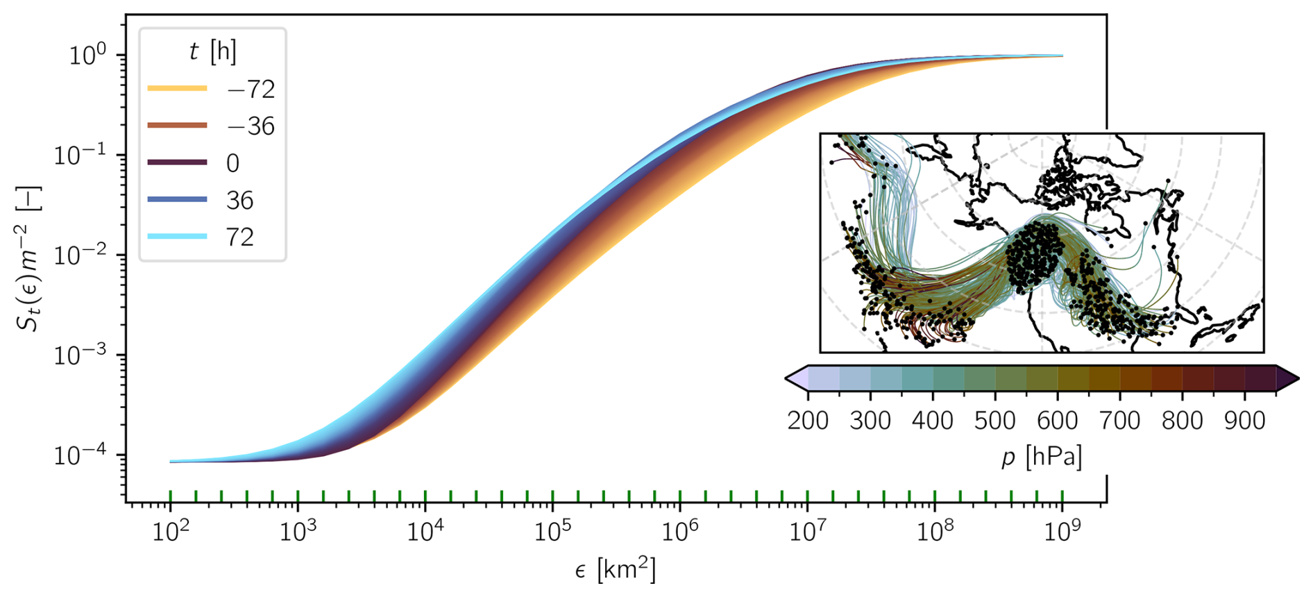
Figure 3 Normalized sum of pointwise diffusion similarities S_t(ϵ)m⁻² plotted versus diffusion bandwidth ϵ on a log–log scale for trajectories initialized on 2 May 2016 at 00:00 UTC. Green horizontal axis ticks indicate evaluated values of ϵ. Inset: trajectories in stereographic projection with vertical coordinate (p) color-coded. Parcel locations at $t=-\mathrm{72},\mathrm{0},\mathrm{72}\mathrm{h}$ as black dots. Only every 50th trajectory is shown for clarity.

In the example presented here, the curve for the initialization time t=0 h has the highest slope, which is because points are placed approximately in a regular three-dimensional grid (see Sect. 3.2). With increasing $\left|t\right|$ in both positive and negative direction, slopes reduce similarly, but curves for positive t saturate earlier. Therefore, the point cloud traced by forward trajectories (t>0 h) stays more densely packed than the same point cloud traced by backward trajectories (t<0 h). Hence, while $d\left(\mathrm{72}\mathrm{h}\right)\approx d(-\mathrm{72}\mathrm{h})$, $\mathrm{\ell }\left(\mathrm{72}\mathrm{h}\right)<\mathrm{\ell }(-\mathrm{72}\mathrm{h})$ (recall that ℓ(t) approximates a grid length and is therefore inversely related to density).

The inset illustrates what is happening: not only do the air parcels diffuse more rapidly horizontally before entering the blocking region compared to after, they also tend to spread to a larger degree in the vertical. A larger spread is related to a smaller density of the points in space and thus larger ℓ. The slope of individual curves is hard to determine from Fig. 3, which is why both d(t) and ℓ(t) are displayed for the whole life cycle of the blocking and the according 3 d forward and backward trajectories in Fig. 4. The data are ordered according to the initialization time along the vertical axis and according to the trajectories' time steps along the horizontal axis. Since trajectories are initialized every 6 h and trajectory data are hourly, white lines with a slope of $\mathrm{1}/\mathrm{6}$ indicate isochrones. Data belonging to the initialization date 29 April 2016 at 06:00 UTC have been omitted due to the low number of trajectories.

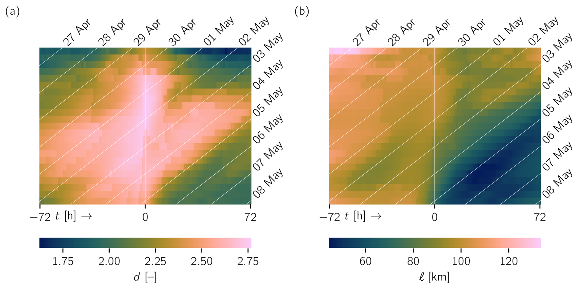
Figure 4 (a) d(t) and (b) ℓ(t) plotted as a function of initialization time (23 initializations, vertical axis) and time step (144 time steps from −72 to +72 h, horizontal axis) for the Canada 2016 case. Data corresponding to trajectories initialized on 29 April 2016 at 06:00 UTC have been removed. White diagonals indicate isochrones (all 00:00 UTC). Vertical white line indicates initialization time.

The dimension heuristic d(t) is higher the closer the air parcels are in time to the initialization configuration (t=0 h). Even then, however, the theoretically achievable dimension of 3 is not reached, which is a boundary artifact, since for points near the boundary, the Gaussian function in Eq. (9) is not fully resolved. This is also why a higher number of trajectories leads to higher values of d(t). Furthermore, Fig. 4a bears testimony to the fact that points tend to arrange more two-dimensionally the further they get away from the initialization time, though two distinct regions may be identified, where this is not the case.

Trajectories passing through the blocking during its late maintenance phase (≈ 3 May; lower center left region in the plot) exhibit a higher dimensionality during their journey into the blocking (t<0), and trajectories passing through the region during its early maintenance phase (≈ 2 May; upper center right region in the plot) exhibit an increased dimensionality during their journey out of the region (t>0). The size of the blocking is of first-order importance for this phenomenon, since high-pressure regions suppress both horizontal and vertical motion (at least in their centers; Ehstand et al., 2021). The larger the blocking, the larger the fraction of air parcels that are under its influence.

Inspection of the individual trajectories confirms that the quasi-stationary flow field reduces the amount of filamentation the point cloud is subjected to. This is because both spatial and temporal small-scale variability will shear – and thus filament – a spatially extended point cloud. In contrast, the air masses traced here behave more like a rigid body being translated and rotated by the lateral large-scale jet and the flow inside the blocking. Recall that d(t) is scale-invariant and isotropic contraction/expansion will, therefore, not change d(t) (see Sect. 2.5). These assessments agree with those made by Ehstand et al. (2021) using similar trajectory-based methods, though on a larger scale and disregarding the vertical dimension.

The level sets of d coinciding with the isochrones for $\mathrm{2.4}>d>\mathrm{2.2}$ in the bottom right of panel (a) in Fig. 4 indicate that several traced air masses that pass through the blocking from 2 May onwards experience a considerable decrease in d roughly at the same time, on ≈5 May at 00:00 UTC. The associated straining motion is related to the disintegration of the blocking and its accompanying lateral wind bands, followed by the reestablishment of the zonal jet. The reorganization of the large-scale flow field exposes the air masses to considerable shear, effectively filamenting the individual point clouds and reducing d(t).

The density measure ℓ(t) shown in Fig. 4b sheds more light on the spatial nature of the investigated trajectories. Importantly, ℓ(t) does not measure the general density of the point clouds (cf. Fig. A2 in Appendix A for mean nearest-neighbor point distances) but rather the inverse density of the points X_t populating 𝕏_t, respecting its dimension. This explains why ℓ(t) does not assume its lowest values uniformly at t≈0, where values equate to roughly 105 km, in agreement with the initial point generation.

The approximated grid length ℓ(t) tends to be lower for forward trajectories compared to backward trajectories. This is especially true for trajectories initialized during the second half of the blocking's life cycle. In Fig. 4b, we find coincidence of level sets of ℓ with isochrones between 1 and 2 May in the bottom left of the plot and around 5 May in the bottom right of the plot. In both cases, ℓ decreases with t, in the first instance with only a slight change in d and in the second instance with a concurrent decrease in d. Hence, the first case hints at isotropic contraction of the point cloud, which is caused by the traced air parcels' arrival in the blocking. For the second instance, the straining imposed on the point cloud of air parcels by the reorganizing flow field makes 𝕏_t appear more two-dimensionally without (sufficient) concurrent isotropic expansion, such that ℓ(t) decreases.

All in all, evolution of the air parcel point clouds traced by the trajectories can be differentiated with respect to the blocking's life cycle: parcels passing through the blocking during onset experience filamentation and straining in both directions in time away from the initialization time (t=0) but are a little more densely packed after leaving the blocking (t>0), which is partially due to a smaller vertical extent. Parcels passing through the blocking during its maintenance phase experience less straining, especially once inside the blocking, but become more densely packed. And parcels passing through the blocking during its decay experience strong and abrupt filamentation upon the blocking's disintegration, which coincides with a decrease in both d and ℓ.

The filamentation of 𝕏_t can also be understood from a more theoretical perspective. Under the influence of the disintegrating blocking, the air masses exhibiting a rapid decrease in d and ℓ undergo material elongation due to the well-researched enstrophy cascade present in turbulent systems with two-dimensional configuration, which is an approximation of the atmosphere due to the scale difference between horizontal and vertical motion (Ditlevsen, 2010; Boffetta and Ecke, 2012). Such an enstrophy cascade to smaller scales and an energy cascade to larger scales involve the elongation and eventual scattering of vortical structures, which explains a decrease in dimension towards d=2. The reconfiguration of the jet stream from a wavy shape (energy at high wavenumber) to a more zonal one (energy at low wavenumber) supports this hypothesis.

The vortex scattering represents a break-up of stability aggregated during the blocking onset and maintenance. The quasi-stationarity of trajectories visible mainly in the maintenance phase of the blocking has to come to an end eventually, already from an entropy perspective. In a structureless, random and turbulent fluid dynamical system, one would expect a more or less symmetric distribution with respect to distance from t=0 in d(t) (see Fig. 4a). Thus, the stability attributed to blocking mainly with respect to flow configuration also seems to be applicable to the material air parcels passing through the region.

4.1.2 Coherent air streams

In order to objectively identify WCB air streams stabilizing the blocking as hypothesized by Steinfeld and Pfahl (2019), we construct the averaged diffusion operator Q_ϵ using m= 11 774 backward trajectories initialized in the blocking region on 2 May 2016 at 00:00 UTC (−72 h $\le t\le \mathrm{0}$ h) for a range of values of ϵ between 2×10⁴ and 1×10⁶ km², the range for which the curve of S_t(ϵ) over ϵ appears linear in a log–log plot (see Fig. 3). For boundary point detection, we apply a value of α=10³ km, which is on the conservative (higher) side of $\sqrt{\mathit{ϵ}}$ for the given range of values of ϵ, and find that the edge lengths of the resulting simplicial complexes at any t stay between 10² km and 10³ km (see Fig. A3).

The resulting spectrum of ${\mathbf{L}}_{\mathit{ϵ}}=({\mathbf{Q}}_{\mathit{ϵ}}-\mathbf{I})/\mathit{ϵ}$ is shown in Fig. 5a. We show the spectrum of L_ϵ instead of Q_ϵ because ϵ controls how close Q_ϵ is to the identity matrix (cf. Fig. 3) and, hence, how close the eigenvalues are to 1. The largest eigenvalues are close but not equal to zero, which is caused by the application of boundary conditions to the normalized matrices ${\widehat{\mathbf{P}}}_{\mathit{ϵ},t}$ before averaging them to obtain Q_ϵ. We identify a moderate spectral gap after the sixth eigenvalue (disregarding spectral gaps at $i=\mathrm{2},\mathrm{3}$ in order to achieve sufficient detail) and perform k--means clustering of the data points into seven clusters in the coordinate space spanned by the first six eigenvectors using a value of $\mathit{ϵ}=\mathrm{5}\times {\mathrm{10}}^{\mathrm{4}}$ km². We found that the resulting clusters are remarkably robust to variation of ϵ and the number of clusters.

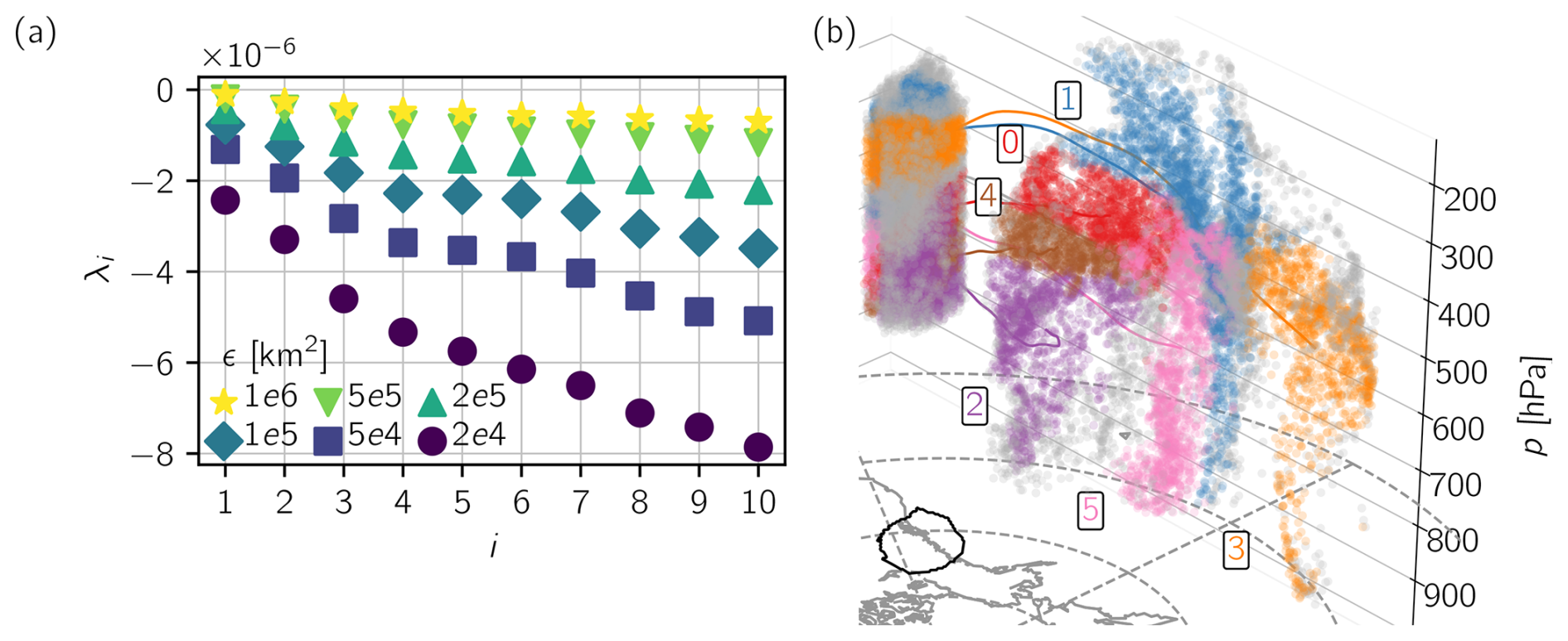
Figure 5 Coherent sets for backward trajectories initialized on 2 May 2016 at 00:00 UTC. (a) The 10 largest eigenvalues of ${\mathbf{L}}_{\mathit{ϵ}}=({\mathbf{Q}}_{\mathit{ϵ}}-\mathbf{I})/\mathit{ϵ}$ for various values of ϵ. (b) Clustered trajectories for $\mathit{ϵ}=\mathrm{5}\times {\mathrm{10}}^{\mathrm{4}}$ km²: colors and according numbers show the clustering, points are shown for t=0 and $t=-\mathrm{72}$ h, and lines show average trajectories. Residual set in gray. Horizontal coordinates are in stereographic projection. Black contour shows location of identified blocking at t=0 h.

Figure 5b depicts the resulting clusters differentiated by colors. Shown are locations of the air parcels at both the initialization (t=0 h) and the end point ($t=-\mathrm{72}$ h) as well as each cluster's average trajectory (calculated by all points' average location for each time step). The gray cluster represents the set of points for which all eigenvectors of Q_ϵ simultaneously show values close to zero. This implies that the points in the gray cluster are, most of the time, boundary points, which is why we regard the gray cluster as a residual cluster. The remaining six clusters show remarkable coherence upon visual inspection of the points at each t, though the coherence tends to be stronger the closer the parcels are to the initialization, which seems natural as the points more strongly resemble a three-dimensional continuum the further they have traveled towards their initialization point in the blocking.

We give estimates of the coherence of the resulting clusters by showing their exit probabilities as defined in Eq. (8), along with the exit probabilities of 100 random test sets as described in Sect. 2.4. Figure 6 confirms that the coherent sets found using the presented methodology are considerably more coherent than the randomly chosen test sets. The residual set stands out starkly, which gives us further confidence in discarding it for the ensuing analysis. Remarkably, the coherence of the sets as measured by the exit probabilities correlates negatively with the clusters' size for the test sets but does not for the coherent sets found. The largest eigenvalues of the restricted matrices ${\left[{\mathbf{Q}}_{\mathit{ϵ}}\right]}_{{\mathcal{I}}_k,{\mathcal{I}}_k}$ displayed in Fig. S5a present the same picture, though the differences between coherent and test sets are smaller.

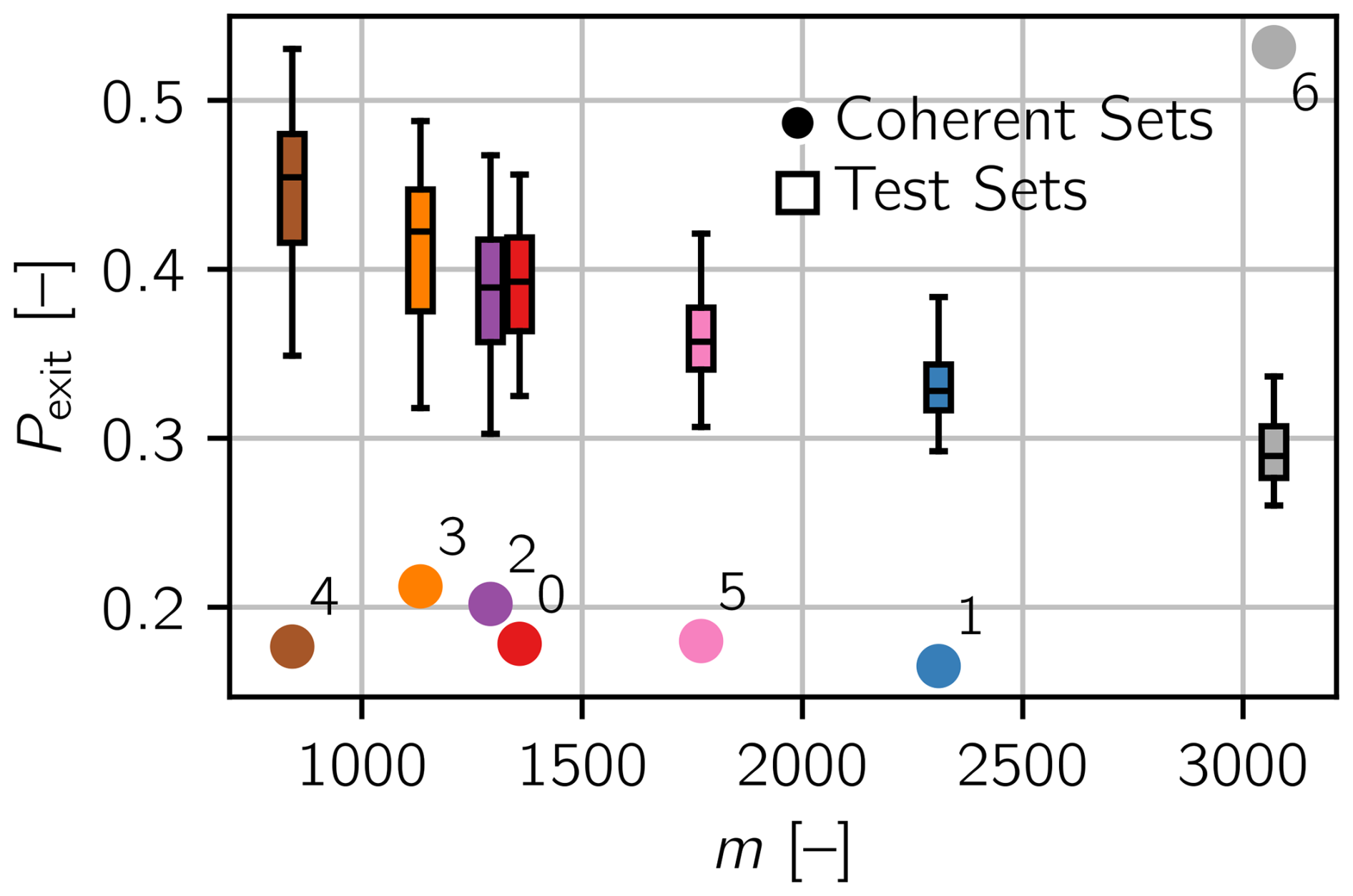
Figure 6 Exit probabilities P_exit(ℐ_k) for each of the clusters shown in Fig. 5 (full circles). For each of the clusters, the distribution of exit probabilities of 100 randomly generated test sets of the same size is presented by a box-and-whisker plot. These show the median (horizontal line), first and third quartiles (box limits), and the farthest data point lying within 1.5 times the interquartile range from the box (whiskers).

Figure 7a provides insight into the dynamical properties of the individual clusters, though the gray residual set has been omitted. Importantly, we identify a considerable increase in potential temperature for the air parcels in the purple (2; note that the clusters' labels are arbitrary, since k--means clustering does not imply a ranking between clusters) and pink (5) clusters. The purple cluster starts at the eastern flank of X₋₇₂ in the lower troposphere and travels to the northern, lower flank of X₀ undergoing significant upward motion. In absence of other strong diabatic effects, the large positive change in potential temperature can only be caused by latent heating, which is confirmed by its change in specific humidity (cf. Fig. S3). The change occurs mainly during the 24 h leading up to the arrival in the blocking, which is in contrast to the pink cluster, which experiences latent heating earlier. The magnitude of the heating in the pink cluster is also a little lower, since the cluster initially extents in the vertical to a larger degree. The cluster undergoes vertical compression over the course of the 3 d and ends up in the lower southeasterly corner of the low-PV anomaly region, adjacent to the purple cluster.

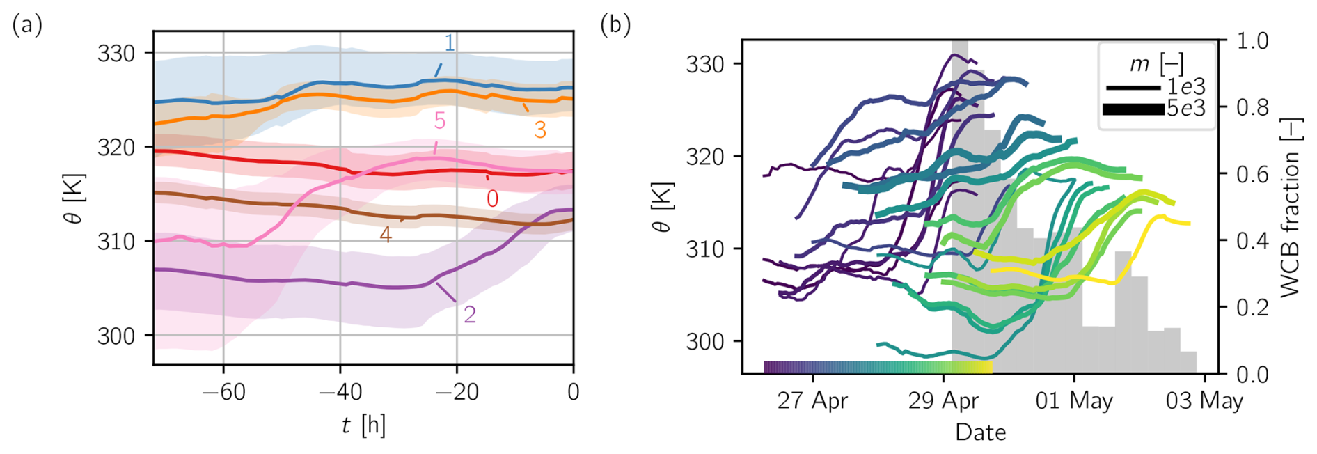
Figure 7 (a) Median (line) and interquartile range (shading) of potential temperature distribution among individual clusters from Fig. 5. Boundary point cluster (gray) not shown. (b) Median (line) of potential temperature distribution among clusters that exhibit a difference between initial and end values larger than 5 K for different initialization times indicated by line color. Line thickness is according to the number of trajectories in a cluster (m). Gray bar chart in the background shows the ratio between the number of trajectories contained in WCB clusters and the total number of trajectories for each arrival (initialization) time.

The diabatic lifting of both clusters is due to large-scale ascent typically associated with warm fronts. The pink cluster “overtakes” the purple, red (0) and brown (4) clusters as it reaches the region of strong lower-tropospheric winds earlier and remains in the blocking region after its earlier arrival while slowly progressing under anticyclonal movement. The behavior of both clusters strongly suggests the existence of a warm conveyor air stream caused by the strong adjacent surface low (cf. Fig. 2a), which supplies the blocking with anomalously low PV air masses at two distinct points in time. We remark that cross-isentropic ascent may in principle also be caused by small-scale convection (Zschenderlein et al., 2020), but such events are on spatial scales unresolved by our data, which makes it unlikely these processes are responsible for the behavior seen in the coherent sets here. Forward trajectories for the same initialization time exhibit synchronized behavior similar to the example discussed next and will thus not be discussed here. Changes in potential temperature are almost exclusively negative, hinting at radiative cooling typical for air masses in the upper troposphere. The synchronization of movement is also indicated in Fig. 4 – the air masses barely separate and are thus rather similar both geometrically and dynamically.

To understand the occurrence of WCBs across the lifetime of the blocking, we automatically identify them for each set of trajectories. To that end, we apply our algorithm with α=10³ km, $\mathit{ϵ}=\mathrm{5}\times {\mathrm{10}}^{\mathrm{4}}$ km² to backward trajectories initialized at each of the 6-hourly time steps. We identify the spectral gap we are interested in by finding the largest absolute difference between two sequential eigenvalues, starting from the third eigenvalue. For the trajectory clusters identified, we select those whose median potential temperature 3 d before arriving in the blocking ($t=-\mathrm{72}$ h) is at least 5 K below the median potential temperature when arriving in the blocking (t=0 h). The results are shown in Fig. 7b. We note that this diagnostic suffers from the ambiguity of the concept of the spectral gap and, hence, the number of clusters selected, which is why we also show the clusters' sizes (number of trajectories in a cluster; m).

The strongest large-scale lifting and, thus, diabatic heating occur during the onset of the blocking, governed by the strong surface cyclone west of it. This is in accordance with findings from Miller and Wang (2022), who highlighted diabatic heating as a key mechanism for the onset of Pacific blockings (though, again, they only studied winter cases). We find coherent bundles of trajectories with median changes in potential temperature of up to 20 K within a day, which does not seem to be atypical (e.g., Madonna et al., 2014). In that phase, the majority of trajectories are part of some cluster featuring considerable heating, as indicated by the gray bars in the background of Fig. 7b. The continuous decrease in the ratio of such trajectories inside WCBs to the total number of trajectories comes about for four different reasons. The first reason is the general enlargement of the blocking. The quasi-stationary nature of blockings implies that air parcels can get “trapped” inside it (see also the following example), which means that even parcels that have experienced latent heating at some point will not be identified as such as soon as this heating is more than 3 d past. The second reason is the decay of the neighboring surface cyclone, which is the dynamic cause of the WCBs. The third and fourth reasons are unavailability of moisture as the blocking travels over land and large-scale subsidence caused by the blocking itself. Higher occurrence of WCBs during onset is confirmed by existing research (Steinfeld and Pfahl, 2019; Hauser et al., 2023)

The plot also shows that WCB clusters identified in sets of trajectories initialized at different times tend to exhibit strong latent heating at the same time. This is because WCBs are synoptic-scale structures, extensive in both space and time. Their intermittent occurrence is linked to presence and absence of surface cyclones and their corresponding warm fronts (Madonna et al., 2014; Catto et al., 2015). Note also that the general decrease in potential temperature is related to the blocking traveling poleward.

In addition to identifying WCBs, we want to further understand the behavior of d(t) and ℓ(t) discussed in Sect. 4.1.1. To that end, we apply our algorithm to m=9882 connected forward and backward trajectories ($-\mathrm{72}\mathrm{h}\le t\le \mathrm{72}\mathrm{h}$) passing through the blocking on 4 May 2016 at 00:00 UTC, which is close to the end of its life cycle, using the same range of values for ϵ and the same value for α (see Fig. A3 in Appendix A for distribution of α hull edge lengths). We identify a moderate spectral gap after the fourth eigenvalue (see Fig. S4a) and again apply k--means clustering using $\mathit{ϵ}=\mathrm{5}\times {\mathrm{10}}^{\mathrm{4}}$ km² but looking for five clusters this time. The resulting clusters are shown in Fig. 8a 3 d before and after initialization ($t=-\mathrm{72}$ and t=72 h) along with their mean trajectories and the blocking's location at t=0 h. A residual cluster has been removed from Fig. 8a, c and d but is shown in b. Given its average exit probability at the upper extremal end of the distribution, we are confident in its classification as residual despite is large size. It contains trajectories that are at the boundary often but also trajectories that are very well mixed (especially in the horizontal), which is a feature observed more often in combined forward and backward trajectories. Our alternative metric (the largest eigenvalue of the restricted matrices) offers the same indication (cf. Fig. S5).

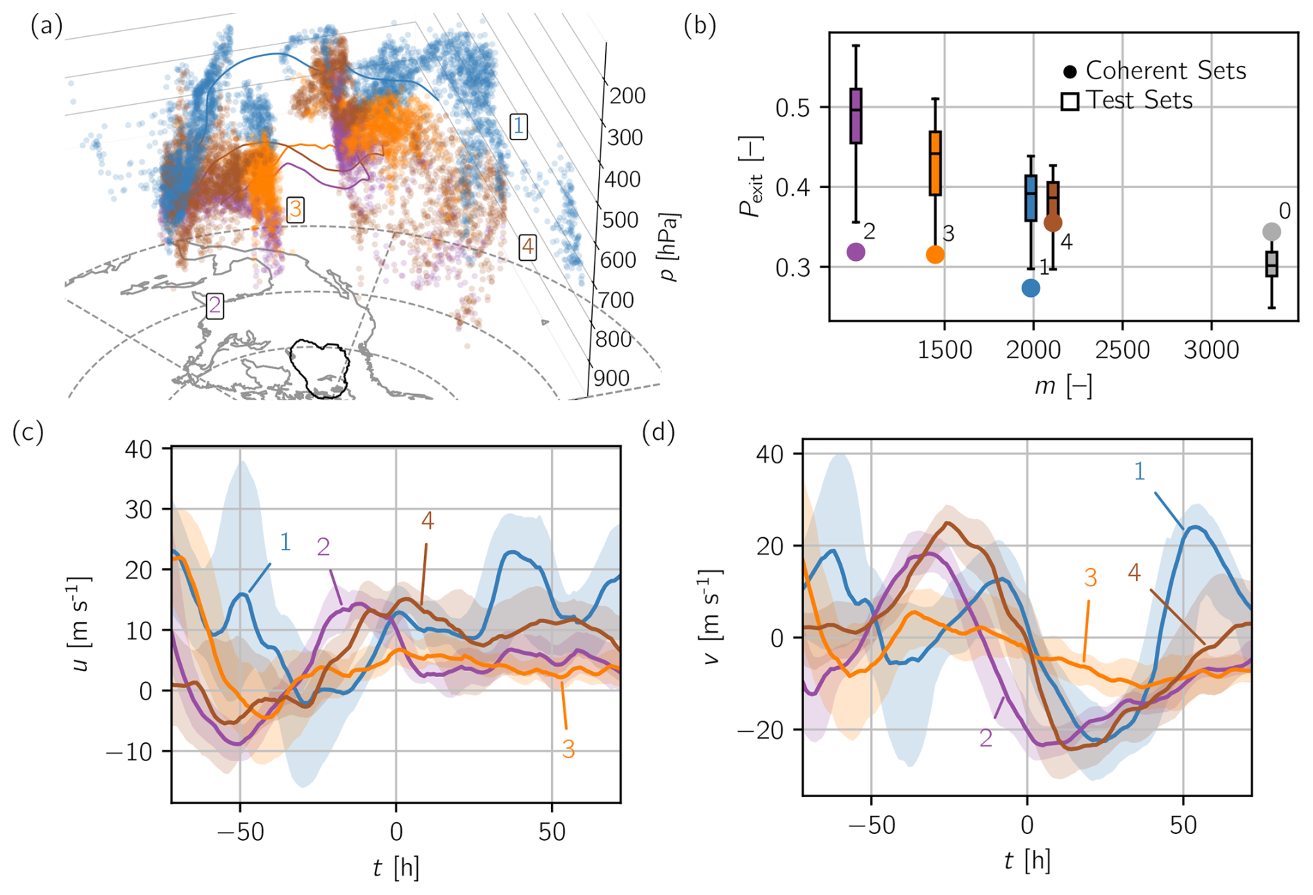
Figure 8 (a) Coherent sets for combined forward and backward trajectories initialized on 4 May 2016 at 00:00 UTC. Points are shown for $t=-\mathrm{72}$ h (right bulk) and t=72 h (left bulk). Black contour shows location of identified blocking at t=0 h. Horizontal coordinates are in stereographic projection. (b) Exit probabilities P_exit(ℐ_k) for each of the clusters shown in (a) and a residual cluster (full circles). For each of the clusters, the distribution of exit probabilities of 100 randomly generated test sets of the same size is presented by a box-and-whisker plot. These show the median (horizontal line), first and third quartiles (box limits), and the farthest data point lying within 1.5 times the interquartile range from the box (whiskers). Panels (c) and (d) show the median (line) and interquartile range (shading) of horizontal velocity components. The residual cluster (gray) has been removed from (a), (c) and (d).

In contrast to the example above, the clusters are separated to a larger degree in the vertical, which is caused by predominantly synchronized movement in the horizontal as well as absence of any updrafts, as will be shown below. The air parcels move considerably less far both in the horizontal and in the vertical, especially during their approach into the blocking. In fact, the bulk of the air parcels are already within or in close vicinity of the anomaly region 3 d before – some are even east of the blocking. Therefore, it comes as no surprise that latent heating does not play a role in the air parcels traced (see Fig. 7b).

The vast majority of parcels stays in the upper troposphere between 300 and 600 hPa the whole time. While the orange (3) cluster undergoes descending motion throughout, the purple (2) and brown (4) clusters perform a moderate ascent into the blocking, though all clusters descend after passage through the blocking, which is no surprise since the initialization points populate the whole upper troposphere, and passage through the tropopause is generally unlikely.

To investigate the movement of the parcels more closely, Fig. 8c and d display the horizontal velocities of the respective clusters. Most of the air parcels experience zonal velocities below a magnitude of 10 m s⁻¹ throughout their journey but especially during their approach ($-\mathrm{48}\mathrm{h}<t<\mathrm{0}\mathrm{h}$), which reflects the blocking's eponymous obstruction of mid-latitudinal westerlies. The obstruction also explains the larger meridional velocity magnitudes visible in Fig. 8c.

Judging from both Figs. 4 and 8, the 6 d journey of the clusters (or more precisely, the air parcels) can be roughly divided into four phases:

1. Day 1 (1 May; $-\mathrm{72}\mathrm{h}<t<-\mathrm{48}\mathrm{h}$). The purple (2) and the orange (3) clusters are already in the vicinity of the blocking region, while the brown (4) and blue (1) clusters contain “tails” that gradually travel eastward. The brown cluster is quite distributed, which is also imprinted in its relatively high escape probability (see Fig. 8b). Those parcels already within the vicinity of the blocking are subject to the quasi-stationary anticyclonal flow field, such that 𝕏_t seems to curl in. The purple cluster is located on the southern flank of the blocking and, therefore, experiences westward velocities. The increase in d and a decrease in ℓ (see Fig. 4) are a result of convergence horizontally and vertically and the advent of the trailing air parcels into the blocking, reducing the amount of filamentation of 𝕏_t.

2. Days 2–3 (2–3 May, $-\mathrm{48}\mathrm{h}<t<\mathrm{0}\mathrm{h}$). All four clusters are quite close horizontally, but both the purple and the blue clusters still gather some trailing parcels vertically, resulting in the continued convergence and increase in d. Shearing deformation is not present; rather all clusters stay within the blocking region, sequentially experiencing the same velocities. In Fig. 8, both horizontal velocities show parallel curves for the different clusters, indicating a simple time shift between similar movements.

3. Day 4 (4 May, $\mathrm{0}\mathrm{h}<t<\mathrm{24}\mathrm{h}$). The movement pattern of the different clusters continues under addition of (mostly) meridional translation as the air masses travel out of the blocking into the northerly jet on the blocking's eastern flank. Vertical motion is almost non-existent, but transport out of the blocking starts to shear 𝕏_t, reducing d and ℓ.

4. Days 5–6 (5–6 May, $\mathrm{24}\mathrm{h}<t<\mathrm{72}\mathrm{h}$). Under combined isentropic downward motion caused by movement out of the high-pressure region, all clusters get strained horizontally along the cyclonic flow field to the southeast of the blocking's last position above the Great Lakes. Both trailing air parcels belonging to the (purple) cluster closest to the surface and leading air parcels belonging to the (blue) cluster furthest from the surface experience a strong westerly flow, caused by a cyclone located above northeastern Canada. Both of these effects elongate and disperse 𝕏_t, resulting in a rapid decrease in both d and ℓ as the anticyclonic vortex has been scattered by neighboring cyclones working towards the reestablishment of the westerly jet stream.

4.2 Northern Europe 2017

The second example revolves around a blocking originating over the North Atlantic during winter, suggesting different characteristics than the case discussed above. The boreal winter 2016/2017 was marked by a number of severe cold spells over central and eastern Europe and Russia, accompanied by warm conditions in the Arctic, a low sea ice extent especially in the Barents–Kara Sea and an exceptionally weak polar vortex. The conditions were likely both favored and enhanced by notably high blocking activity throughout mid-latitudinal Eurasia (Tyrlis et al., 2019). The conditions drastically influenced the lives of millions of people (Anagnostopoulou et al., 2017; Demirtaş, 2022; Kostopoulou, 2023).

The blocking investigated here was just the last in a number of strong European blockings but has reached a considerable extent both spatially and temporally. This suggests low-frequency variability as a possible cause for onset as concluded by Nakamura et al. (1997), though Miller and Wang (2022) pointed to high-frequency components as key factors. Our blocking data set recognizes blocked grid points between 23 January 2017 at 12:00 UTC and 30 January 2017 at 12:00 UTC. Figure 9 shows the synoptic conditions over the region of influence for three selected times representative of onset, maintenance and decay of the blocking (a video containing synoptic conditions for all time steps is provided in the Supplement).

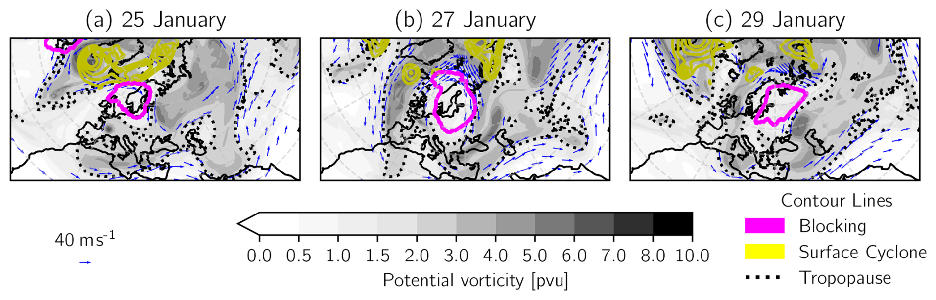
Figure 9 Synoptic conditions at three time instances (all at 00:00 UTC) during the northern Europe 2017 case. Upper-level PV (shaded), 2 pvu contour (tropopause) in black, upper-level wind (blue vectors, only shown for wind speeds larger than 30 m s⁻¹), surface cyclones (sea level pressure; yellow contours from 970 to 990 hPa every 5 hPa; note the difference to Fig. 2) and blocking region (magenta contour; see Sect. 3.1 for definition). Upper-level fields are vertically averaged between 500 and 150 hPa. Note that horizontal wind velocity is indicated by the quivers' length. Denser quivers towards the poles result from denser longitudes.

During onset (a) the low-PV anomaly developed as a vast region of low pressure over the North Atlantic and the Arctic lets subtropical air travel north, disrupting the jet stream. Blocking formation can be seen as an example of anticyclonal Rossby wave breaking, which is in agreement with Miller and Wang (2022). The blocking progressed remarkably little over the course of the ensuing week and severely obstructed the usual westerly flow of air. A typical Ω-blocking configuration is visible in (b) as two regions of high PV develop at the lower lateral flanks of the low-PV anomaly region. This leads to a considerable deflection of the jet stream, and low-PV air masses are guided northwards on the western flank just as high-PV air masses are guided southward on the eastern flank of the blocking along strong meridional wind bands.

The blocking eventually traveled eastward, gradually dispersing over the Ural Mountains and Siberia (c). Insights gained from the previous case study corroborate the argument of Steinfeld and Pfahl (2019) that WCBs tend to strengthen the negative PV anomaly, which would imply that its absence makes decay of the blocking more likely. In the present case, the blocking persisted for an extended amount of time over Scandinavia and eventually dissolved over mainland Russia, such that a possible hypothesis is that the decay of the blocking coincided with the cessation of WCBs' feeding due to a lack of moisture, a weakening of the adjacent surface cyclone and large-scale subsidence.

To analyze air stream coherence, we apply the same value for the scale parameter κ=15 km hPa⁻¹ and obtain between 50 and 19 200 initial points (see Fig. A1). The variation of κ is, again, inside a moderate range of 12.09 to 19.82 km hPa⁻¹ and does not show a great influence on the eventual clustering of trajectories. Temporal evolution of κ indicates relatively weaker motion in the vertical the later the trajectories pass through the blocking. Average velocities in both horizontal and vertical direction develop similarly and largely decrease with time, which is related to the presence and absence of WCBs and the traced air parcels' vicinity of the stagnant flow field dominated by the blocking. Mean velocities over the trajectories' whole 6 d time period are provided in Fig. S2.

4.2.1 Trajectory density

We show the estimates of both d(t) and ℓ(t) for the present example in Fig. 10. Data corresponding to trajectories initialized on 23 January 2017 at 12:00 UTC have been removed since the initial point generation resulted in only 50 trajectories. We find that the distributions of d(t) and ℓ(t) over time and across the blocking's life cycle bear some resemblance to the first case, though we note that values are generally slightly higher for both heuristics, which we attribute to the higher number of trajectories. For d(t), we identify maxima of well below 3 for point clouds with the most points (see Fig. 10) and close to the initialization time and recognize a more or less monotonic decrease away from those. Regions of larger d(t) are, again, visible for t>0 h for trajectories initialized during the maturing phase (25–26 January) and for t<0 h for trajectories initialized during the late maintenance phase (27–28 January). This sparks the question of whether the same physical processes are responsible for the observations as in the first case study.

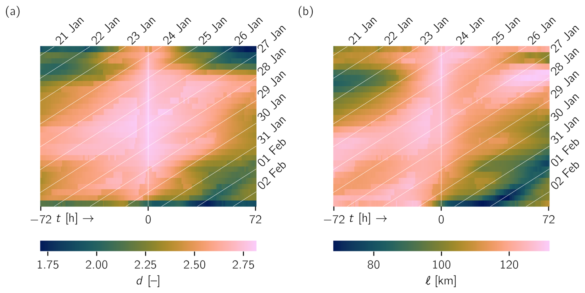
Figure 10 (a) d(t) and (b) ℓ(t) plotted as a function of initialization time (28 initializations, vertical axis) and time step (144 time steps from −72 h to +72 h, horizontal axis) for the northern Europe 2017 case. Data corresponding to trajectories initialized on 23 January 2017 at 12:00 UTC has been removed. White diagonals indicate isochrones (all 00:00 UTC). Vertical white line indicates initialization time.

Onset and early maintenance of the blocking were heavily influenced by the strong low-pressure region to the west of it. Both d and ℓ increase considerably as air is transported into the blocking along the strong wind band on the surface cyclones' eastern flank. Similar to rolling up a fish net (the rotational axis in the p direction), 𝕏_t contracts and increases in dimension as the parcels end up in the blocking and stay there, while the approximated grid length increases slightly. Considerable upward motion supports this process. This is in contrast to the first case study, where ℓ stayed largely constant during this phase. The compressed, almost three-dimensional 𝕏_t stays largely intact and inside the blocking as it stagnates and grows over northern Europe. Consequently, temporal development of d and ℓ in approaching air parcels during the blocking's period of largest extent is also dominated by parcels already in or close to the blocking, such that neither d nor ℓ changes considerably.

The blocking reached its peak extent around 27 January (cf. Fig. A1). Subsequent shrinking means air masses under the influence of the quasi-stationary flow field inside the blocking now escape and come under the influence of a low-pressure center in the upper troposphere at the southeasterly flank of the blocking. This is why forward trajectories initialized around 25–26 January see essentially no decrease in d or ℓ, but those initialized around 27 January do. This is in contrast to the first example case discussed, which showed both a later peak and a slower subsequent decline in size. Disintegration of the blocking and its associated flow field leads to decreases in both heuristics, similar to the first case study, albeit less pronounced.

4.2.2 Coherent air streams

We apply our diagnostic presented in Fig. 7b for the present case to study and summarize the occurrence of coherent air streams featuring latent heating and show results in Fig. 11a. WCBs are found almost exclusively among backward trajectories arriving in the blocking during its lifetime's first half. During that period, however, they make up a considerable share of all trajectories traced. Miller and Wang (2022) also identified diabatic heating as a major cause for blocking onset in the European region.

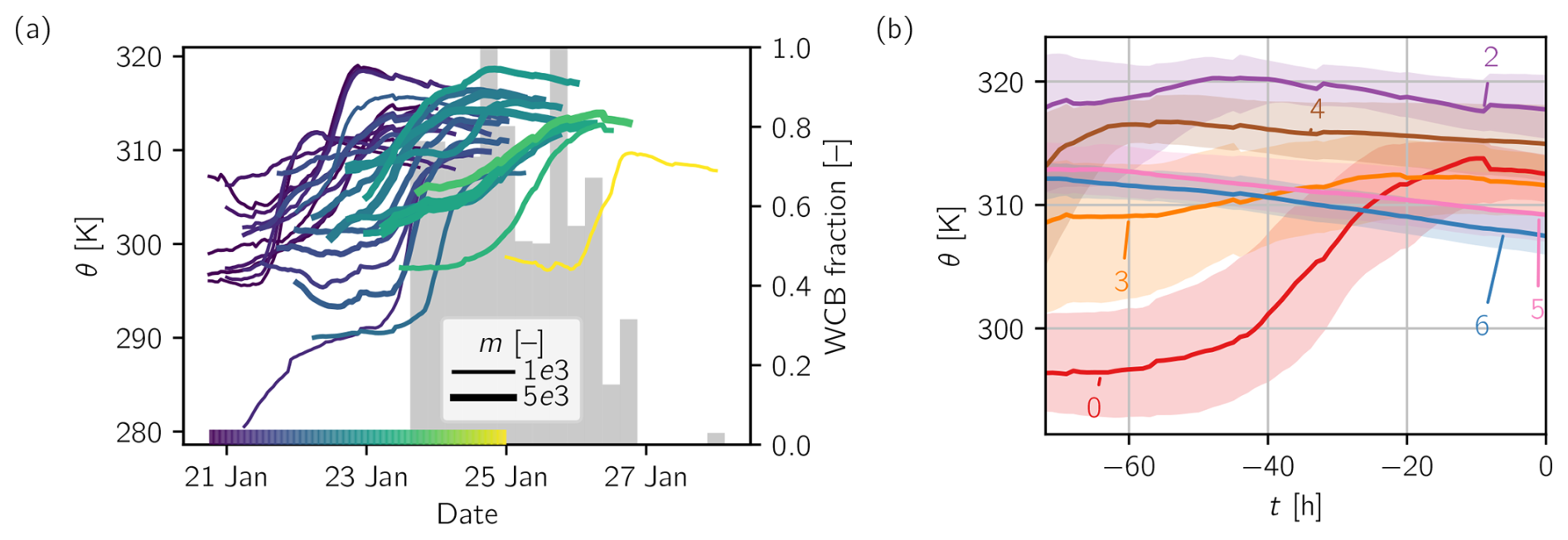
Figure 11 (a) Median (line) of potential temperature distribution among clusters that exhibit a difference between initial and end values larger than 5 K for different initialization times indicated by line color. Line thickness is according to the number of trajectories in cluster (m). Gray bar chart in the background shows ratio between number of trajectories contained in WCB clusters and the total number of trajectories for each arrival (initialization) time. (b) Median (line) and interquartile range (shading) of potential temperature distribution among individual clusters from Fig. 12. A residual (gray) cluster has been removed.

Both example cases presented here feature WCBs (according to our definition: coherent air streams with a 3 d change in median potential temperature of more than 5 K) almost exclusively during the onset and early maintenance phase. In both cases, these are caused by adjacent surface lows. Compared to the first case study, the WCB fraction decreases less monotonically. A possible explanation is that moisture availability is dependent on oceanic sources to a larger degree in winter (Pfahl et al., 2014), but proving this would require moisture source tracking, which is outside the scope of the present study. In comparison to the first evaluation of WCBs, the potential temperature levels tend to be a bit lower in this case, which reflects the different seasons they occurred in. Notably, the second blocking does not show lower levels of potential temperature with time since it does not move to higher latitudes.

As a last demonstration of our methodology, we pick the set of backward trajectories initialized on 26 January 2017 at 18:00 UTC, which we understand as a turning point in the blocking's life cycle in several senses. Firstly, at this point in time the blocking has almost reached its maximum extent, allowing for a total of 18 349 individual initial points. Secondly, from a process-oriented perspective, Fig. 11b reveals that this point in time is the last featuring a WCB with considerable size, but the trajectories also exhibit the behavior responsible for profiles of d and ℓ characteristic of later phases, which will be shown in the following. The synoptic conditions at the selected point in time differ only marginally compared to Fig. 9b.

After calculating boundary points with α=10³ km again (see Fig. A3 for resulting α hull edge length distribution), we identify a moderate spectral gap after six eigenvalues (see Fig. S4b) and select $\mathit{ϵ}=\mathrm{5}\times {\mathrm{10}}^{\mathrm{4}}$ km² to cluster the trajectories. The result is shown in Fig. 12a, where a residual cluster has already been removed for visibility. This residual cluster stands out drastically in Fig. 12b, attaining a very high average exit probability of above 0.5, whereas the other clusters are proven to be a lot more coherent than the randomly chosen test sets. Again, the largest eigenvalues of the restricted matrices show a similar but less clear picture, especially with regard to the residual cluster (cf. Fig. S5).

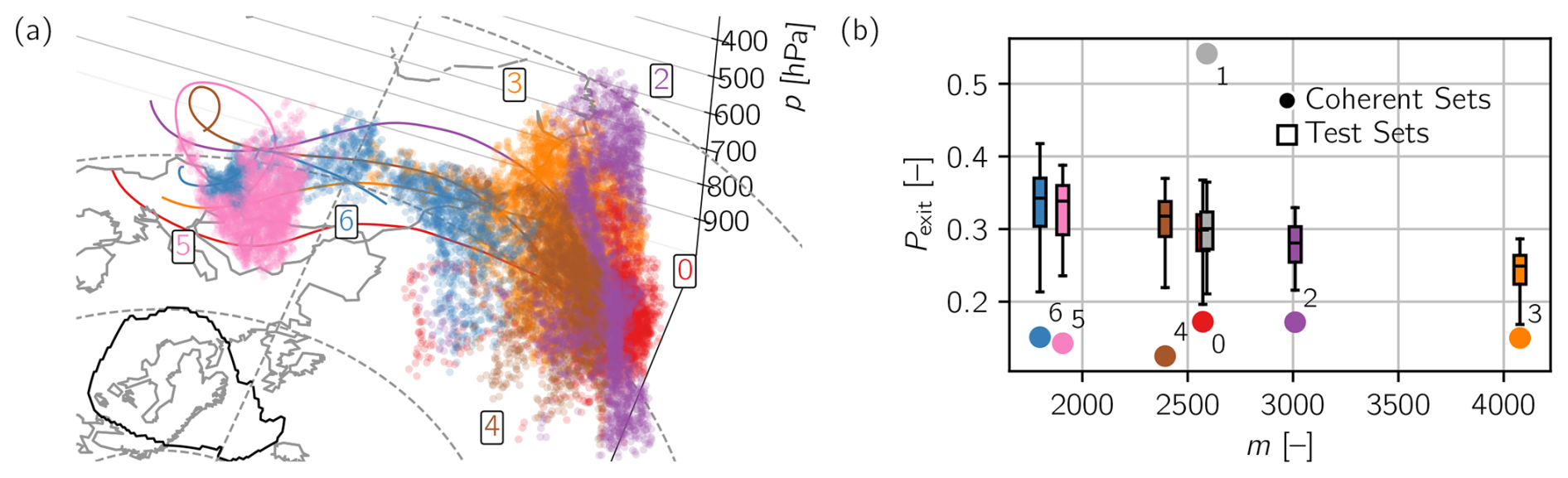
Figure 12 (a) Coherent sets for backward trajectories initialized on 26 January 2017 at 18:00 UTC. Clustered trajectories for $\mathit{ϵ}=\mathrm{5}\times {\mathrm{10}}^{\mathrm{4}}$ km². Points are shown for $t=-\mathrm{72}$ h; black contour shows location of identified blocking regions at t=0 h. One (gray) residual cluster has been removed. Horizontal coordinates are in stereographic projection. (b) Exit probabilities P_exit(ℐ_k) for each of the clusters shown in (a) (full circles) and the residual cluster removed from (a). For each of the clusters, the distribution of exit probabilities of 100 randomly generated test sets of the same size is presented by a box-and-whisker plot. These show the median (horizontal line), first and third quartiles (box limits), and the farthest data point lying within 1.5 times the interquartile range from the box (whiskers).

Note that the positions of the air parcels are only shown at $t=-\mathrm{72}$ h, whereas the blocking's location is shown at time t=0 h. This is because air parcel locations overlap considerably for $t=-\mathrm{72}$ and t=0 h and would therefore be impossible to distinguish.

This time, clusters are separated stronger horizontally, owing to a larger degree of vertical mixing compared to the previous example. Clusters at $t=-\mathrm{72}$ h appear rather filamented (except for the pink cluster (5)) and even feature seemingly disconnected pockets of air (red cluster (0)), which highlights the role the final configuration close to t=0 h plays. The distributions of θ of the individual clusters over time shown in Fig. 11a, however, prove that all but the red clusters are concentrated in the upper levels of the atmosphere. The red cluster, on the other hand, can be identified as one of the WCBs visible in Fig. 11b. Its air parcels undergo latent heating, increasing their median potential temperature by roughly 15 K. Given the fact that the synoptic flow field and general conditions make it likely that the other clusters have a similar “history” and have, thus, undergone a diabatic ascent as well – just earlier – further underlines the importance of latent heating in this case.

The pink cluster consists of air that is already inside the blocking at $t=-\mathrm{72}$ h. During the ensuing 3 d, it performs an anticyclonic rotation characteristic of high-pressure systems (in the Northern Hemisphere). This is visible in Fig. 13, where the horizontal velocity components are displayed in a hodograph for all clusters shown in Fig. 12a. The polar plot enables display of both horizontal velocity components in one graph and makes the circular movement of the pink cluster clear. The blue (6) and brown (4) clusters' arrival in the blocking can be similarly identified by their anticyclonic movement later on, though the curves are a lot less clear. A decrease in zonal velocities reveals that the blue cluster arrives second before the brown, the purple (2) and finally the red.

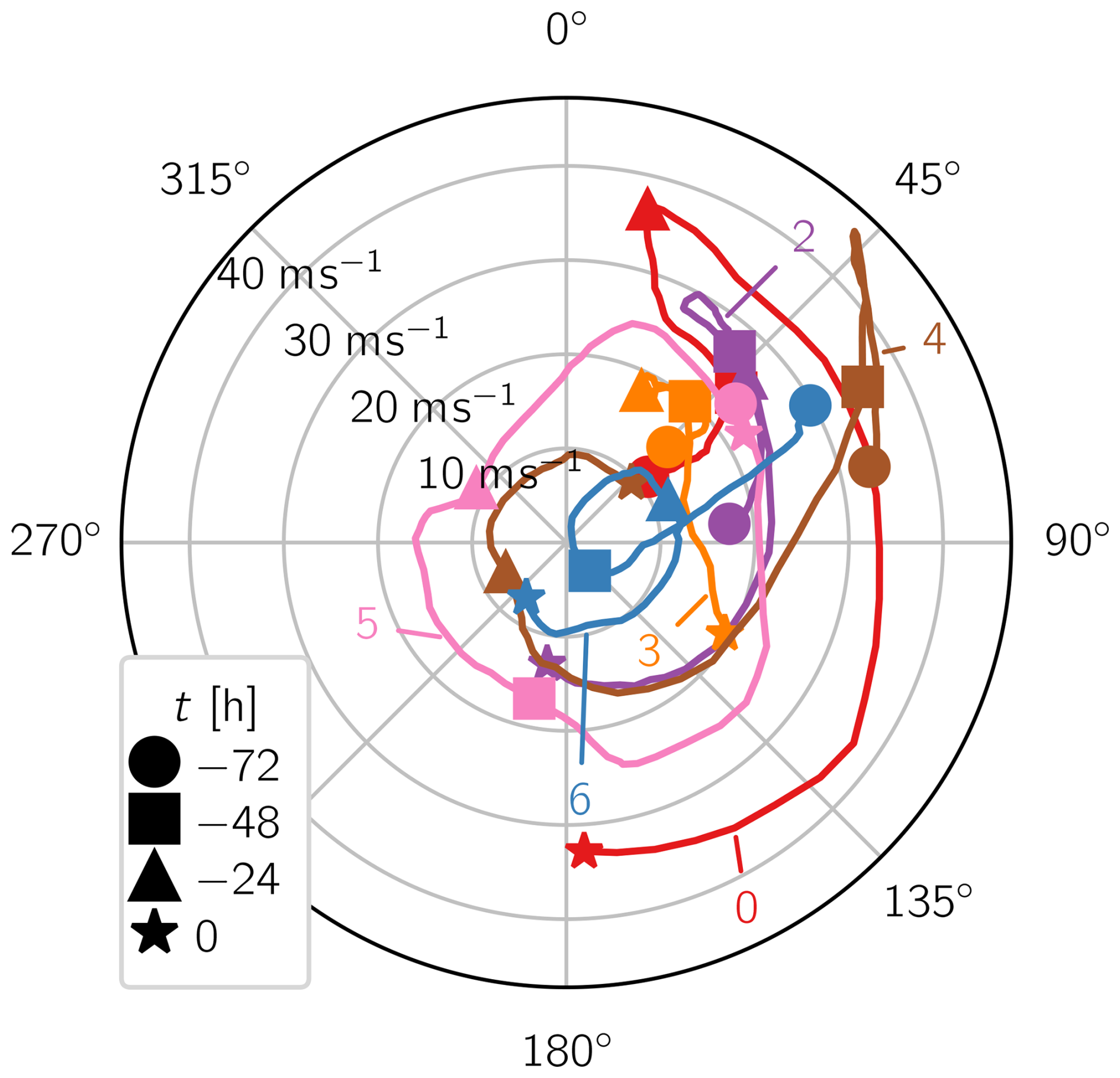
Figure 13 Median horizontal velocities of each cluster from Fig. 12a displayed as a hodograph. 0° corresponds to exclusively northward motion. Markers indicate time steps.

Tracking of the individual clusters confirms the hypothesis formulated in Sect. 4.2.1. The size of the blocking determines when and how long the traced parcels are inside its region of influence and, thus, how densely and to what extent the parcels assemble three-dimensionally at a particular point in time. The present example also demonstrates that the processes discussed do not occur exclusively but can coexist and contribute to the complexity of both individual cases and case-to-case variability.

5 Conclusions

The present study aimed to investigate the occurrence of warm conveyor belts (WCBs) feeding into atmospheric blocking adhering to the notion of spatial coherence. This promised to provide a complementing perspective on WCBs as phenomena of first-order importance for the behavior and development of atmospheric blocking. We also use this case study to prove the methodological value of the mathematical concept of coherent sets, which is an active area of research. To the best of our knowledge, neither the study of WCBs based on their spatial coherence nor the identification of coherent air streams in high-resolution three-dimensional atmospheric trajectories has been carried out thus far.

The adaptation, implementation and advancement of the methodology of Banisch and Koltai (2017) are the core contribution of this work. The developed framework respects the scale dissimilarities of atmospheric motion, handles boundary conditions in a physically consistent manner and provides flexibility for application to geoscientific phenomena on other scales, all while keeping numerical efficiency and ease of application in mind. We employ a quantitative metric of coherence to prove our adaptation is able to identify coherent sets that are drastically more coherent than randomly selected test sets. Broadening the range of phenomena studied in this manner is a subject of future work. To facilitate this, we provide a user-friendly Python package, GeoCS (see “Code and data availability”).

The case studies presented demonstrate our method's capability in finding WCBs based solely on spatial information. Apart from respecting the (arguably) common notion of WCBs as coherent, synoptic-scale air streams, this perspective has the advantage of being able to conceive WCBs as spatio-temporally extended objects in time, similar to atmospheric blockings. More specifically, we found that, on the one hand, air parcels that reach a blocking at a common point in time may have been part of the same or different WCBs and that, on the other hand, individual WCBs can contain air parcels that reach the same blocking at different points in time (see Fig. 7).

The WCBs found in our case studies were generally remarkably distinct from other coherent sets identified, both with respect to their dynamical properties and their pathways. Nevertheless, we did not find a rigorous dichotomy between moist and dry air streams as it might seem when looking at distributions of maximal potential temperature change over all trajectories traced over the whole lifetime of a blocking event (Steinfeld et al., 2022; Steinfeld, 2019; Pfahl et al., 2015). In agreement with existing research, for both of the two blockings investigated, the influence of WCBs was episodic and larger in earlier stages of the life cycle. Our results suggest that this was due to large-scale subsidence, unavailability of moisture and self-containment of air parcels in blockings later in their life cycle. In earlier stages, however, we found that up to 100 % of the air parcels traced were influenced by a WCB at some point.

In addition to clustering trajectories, the presented method provides concise information on the shape of the point cloud represented by the air parcels traced at each point in time. In particular, we introduced the heuristics d and ℓ approximating the dimension and grid length of the point cloud and emphasize that both of these behave considerably differently than linear measures of distances between the points. Given that Lagrangian analysis is ubiquitous, especially in atmospheric sciences, we think that these tools are a valuable contribution.

Applying these heuristics to our case studies showed that the stabilizing effect a blocking has on the synoptic flow field imprints on the coherence of trajectories that flow through it. This happens due to quasi-stationarity, reduced shearing and generally lower velocities. Consistently, strong and abrupt changes in the flow field, such as when a zonal regime reestablishes after a blocking, lead to shearing and filamentation of point clouds.

Given the complexity of the algorithm developed, a climatological evaluation of the effects discussed for the present case studies is non-trivial and, thus, subject of future studies. As mentioned above, we are convinced that the methodological framework presented will give valuable insights for other meteorological (or oceanic) phenomena such as cyclones.

Appendix A: Additional figures

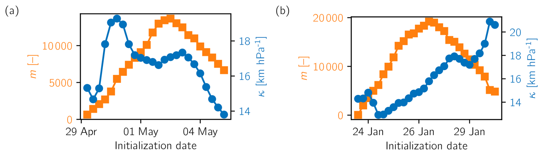
Figure A1 Number of trajectories m (orange squares; left axes) and scale factor κ (blue circles; right axes) calculated over all sets of trajectories and time steps for 3 d forward and 3 d backward trajectories at each initialization date.

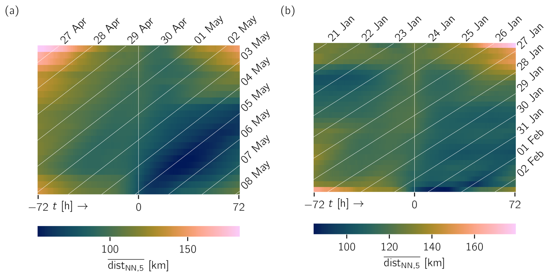
Figure A2 Mean of the five nearest-neighbor distances for each point for (a) the 2016 Canada case and (b) the 2017 northern Europe case. White diagonals indicate isochrones (all 00:00 UTC). Vertical white line indicates initialization time.

Figure A3 A 2D histogram of edge lengths of the α hulls generated by α shapes for the trajectories initialized on (a) 2 May 2016 at 00:00 UTC, (b) 4 May 2016 at 00:00 UTC and (c) 26 January 2017 at 18:00 UTC. Black lines indicate median and quartiles of the distributions for a specific t.