Intermittency in fluid and magnetohydrodynamics (MHD) turbulence analyzed through the prism of moment scaling predictions of multifractal models

In the presence of waves due, e.g., to gravity, rotation, or a quasi-uniform magnetic field, energy transfer timescales, spectra, and physical structures within turbulent flows differ from the fully developed fluid case, but some features remain, e.g., intermittency or quasi-parabolic behaviors of normalized moments of relevant fields, for the most part in that intermediate regime where waves and nonlinear eddies interact strongly. After reviewing some of the roles intermittency can play in various geophysical flows, we present the results of direct numerical simulations at moderate resolution and run for long times. We show that the power law scaling relations between kurtosis K and skewness S found in multiple and diverse environments can be recovered using a selection of existing multifractal intermittency frameworks. Indeed, in the specific context of the She–Lévêque model (She and Lévêque, 1994) generalized to magnetohydrodynamics (MHD) and developed as a two-parameter system in Politano and Pouquet (1995), we find that a parabolic K(S) law can be recovered for maximal intermittency involving the most extreme dissipative structures.

1 Introduction

A word-frequency study performed on research papers centered on a variety of atmospheric issues indicated that the most frequent cloud-controlling factor is turbulence (Siebesma et al., 2009; see also Pumir and Wilkinson, 2016), likely because of its ubiquity but also because it could presumably explain a multitude of somewhat puzzling phenomena that occur at small scales, even if only that of unity-order dissipation at high Reynolds numbers. More recently, fully developed turbulence (FDT) has been associated with the barotropic state of large-scale atmospheric turbulence, with a multiplicative effect due to turbulence on the acceleration of the jet stream and the rapid intensification of hurricanes (Shepherd, 2020; Emanuel et al., 2023; Shaw and Miyawaki, 2024). A similar study for plasma physics might reveal the same feature, i.e., that the complexity of nonlinear phenomena is the dominant property impeding the development of wide-ranging theoretical and modeling techniques of small-scale behavior, thus making the much-needed prediction of disruptions in fusion plasmas difficult, even though this is essential.

Observations of magnetohydrodynamics (MHD) and plasma turbulence in space physics are numerous, with consistent progress in the resolution of satellite instrumentation and now with exploration of the kinetic regime (Fox et al., 2016; Muller et al., 2020). Access to small-scale dynamics through newly launched spacecraft allows, e.g., for a direct evaluation of the dissipation rate spectrum through the measurement of the current and electric fields using the Magnetospheric MultiScale Mission (MMS, He et al., 2019). It has been known for a long time that vortex sheets observed in the first direct numerical simulations (DNS) of turbulence using pseudo-spectral methods could roll up into vortex filaments (Patterson and Orszag, 1971; Siggia and Patterson, 1978) (see Douady et al., 1991, for experimental evidence), whereas in MHD the dynamics lead to complex current and vorticity structures stemming from the sheet destabilization observed in DNS in two dimensions (2-D) (Matthaeus and Lamkin, 1986; Pouquet et al., 1986) and various reconnection processes and possible singularities (Friedel et al., 1997; Kerr and Brandenburg, 1999; Cartes et al., 2009), a topic however which will not be covered in this review (see also, e.g., Bhattacharjee, 2004; Mininni et al., 2008; Zweibel and Yamada, 2009; Daughton et al., 2011; Zhdankin et al., 2013; Lazarian et al., 2020; Oka et al., 2022). Reconnection and the intermittency associated with singularities have been related (Osman et al., 2014), including at high cross-helicity (Smith et al., 2009), and can lead to plasma heating (Marino et al., 2008). Lastly, studies were done to determine the possible development of singular structures in fluids and plasmas in the limit of an infinite Reynolds number, but the problem remains open.

Furthermore, new and accurate observations of Earth's magnetic field were obtained recently from global ocean circulation measurements, potentially leading to a better understanding of oceanic tides, ionosphere–magnetosphere interactions, and their variabilities (Hornschild et al., 2022). Thus, one of the marked properties of velocity and magnetic fields is that of intermittency (and the ensuing anomalous scaling), which is the presence of strong localized structures. These structures can be identified as vortex filaments, Alfvén vortices observed in the solar wind (Wang et al., 2019), or current sheets which experience instabilities such as Kelvin–Helmholtz (KH) ones (see Barkley et al., 2015, for a recent review of KH instabilities), reconnection, and thus dissipation (Matthaeus and Montgomery, 1981; Uzdensky et al., 2010; Faganello and Califano, 2017; Adhikari et al., 2021). An abundance of observations of our close environment points to a complex suite of systems and structures that include turbulence and nonlinearities in MHD as well as plasma instabilities; these also exhibit anomalous scaling and dissipation. See, e.g., Matthaeus et al. (2015), Chen (2016), Galtier (2018), Schekochihin (2022), Balasis et al. (2023), and Marino and Sorriso-Valvo (2023) for recent reviews. Intermittent dissipation in the MHD range has been shown to lead to beam acceleration in the magnetosphere at ionic scales and below (Sorriso-Valvo et al., 2019), and particle acceleration has also been observed with MMS in the vicinity of a reconnection X line, also leading to strong turbulence (Ergun et al., 2020).

There are of course plenty of other manifestations of intermittency, e.g., through non-Gaussian wings of probability distribution functions (PDFs) for Eulerian and Lagrangian fields. Thus, one way of characterizing intermittency in turbulence is through the dual observation of large-scale structures separated by sharp active gradients for both fluids and MHD, which is particularly noticeable in 2-D (Kinney et al., 1995; Meneguzzi et al., 1996; Matthaeus et al., 2015). Another way of quantifying the degree of intermittency of a flow is to measure the anomalous exponents of structure functions, i.e., measure a departure from self-similarity, as done for the solar wind (Burlaga, 1991) and DNS (Politano et al., 1995). MHD intermittency models were built (Grauer et al., 1994; Politano and Pouquet, 1995) (see also Horbury and Balogh, 1997) to explain the observed behavior, but one difficulty resides in the necessity of having a vast amount of data. In this context, after giving the equations in the next section, we will analyze in Sect. 3 numerical results on the third- and fourth-order normalized moments in several systems run at moderate Reynolds numbers for long times and give a justification of the power law behavior between moments in the framework of turbulence models in Sect. 4, together with, in fact, an extension to scaling laws for arbitrary orders. We mention other frameworks for the study of such intermittency in Sect. 5 and draw conclusions in the last section.

2 Equations, parameters, and numerical setup

The incompressible equations for rotating stratified flows in the Boussinesq incompressible framework are

$$\begin{array}{}\text{(1)}& \begin{array}{rl}& {\partial }_t\mathit{u}+\mathit{u}\cdot \mathrm{\nabla }\mathit{u}=-\mathrm{\nabla }p-N\mathit{\theta }\widehat{z}+\mathrm{2}\mathit{u}\times f_{\mathrm{0}}\widehat{z}+\mathit{\nu }{\mathrm{\nabla }}^{\mathrm{2}}\mathit{u}+{\mathbf{F}}_u,\\ & {\partial }_t\mathit{\theta }+\mathit{u}\cdot \mathrm{\nabla }\mathit{\theta }=Nw+{\mathit{\kappa }}_{\mathrm{0}}{\mathrm{\nabla }}^{\mathrm{2}}\mathit{\theta }+F_{\mathit{\theta }},\mathrm{\nabla }\cdot \mathit{u}=\mathrm{0},\end{array}\end{array}$$

with u and θ the velocity and temperature fluctuations (here in velocity units), w the velocity in the direction of imposed gravity and/or rotation (here, the vertical z direction), p the pressure, N and $f_{\mathrm{0}}/\mathrm{2}$ the Brunt–Väisälä and rotation frequencies, and ν and κ₀ the viscosity and thermal diffusivities, taken to be equal (unit Prandtl number). F_u and F_θ are forcing terms. Potential temperature forcing was only used in the quasi-geostrophic (QG) runs (see Sect. 3.2 and Fig. 2), and otherwise it was always set to zero. For N=0 and f₀=0, one recovers the Navier–Stokes (NS) equations with a passive scalar. We also write the MHD equations, again for the incompressible case, and with b the induction in Alfvén velocity units and $P=p+|\mathit{b}{|}^{\mathrm{2}}/\mathrm{2}$ the total pressure:

$$\begin{array}{}\text{(2)}& \begin{array}{rl}& [{\partial }_t+\mathit{u}\cdot \mathrm{\nabla }]\mathit{u}\equiv D_t\mathit{u}=-\mathrm{\nabla }P+\mathit{b}\cdot \mathrm{\nabla }\mathit{b}+\mathit{\nu }\mathrm{\Delta }\mathit{u}+{\mathbf{F}}_u,\\ & [{\partial }_t+\mathit{u}\cdot \mathrm{\nabla }]\mathit{b}\equiv D_t\mathit{b}=\mathit{b}\cdot \mathrm{\nabla }\mathit{u}+\mathit{\eta }\mathrm{\Delta }\mathit{b},\\ & \mathrm{\nabla }\cdot \mathit{b}=\mathrm{0},P_{\mathrm{M}}=\mathit{\nu }/\mathit{\eta }.\end{array}\end{array}$$

Here, η is the magnetic diffusivity and $P_{\mathrm{M}}=\mathit{\nu }/\mathit{\eta }$ is the magnetic Prandtl number. The results described herein have been obtained by integrating numerically these equations with pseudo-spectral accuracy using the GHOST (Rosenberg et al., 2020) and CUBBY (Ponty et al., 2005) codes. In the absence of dissipation (ν=0, η=0, and κ₀=0), the total energy is conserved, together with the cross-helicity and magnetic helicity in MHD and the potential vorticity in the stratified case (see Sect. 3.3 for a definition of helicity).

Given a typical large scale taken as the integral scale L₀ and a characteristic root mean square velocity at that scale u₀, one defines the kinetic and magnetic Reynolds numbers and the Froude and Rossby numbers Fr and  Ro in a standard way, i.e.,

$$\begin{array}{}\text{(3)}& \begin{array}{rl}{R}_{\mathrm{V}}& ={\displaystyle \frac{u_{\mathrm{0}}{L}_{\mathrm{0}}}{\mathit{\nu }}},R_{\mathrm{M}}={\displaystyle \frac{u_{\mathrm{0}}{L}_{\mathrm{0}}}{\mathit{\eta }}},Fr={\displaystyle \frac{u_{\mathrm{0}}}{L_{\mathrm{0}}N}},\\ & Ro={\displaystyle \frac{u_{\mathrm{0}}}{L_{\mathrm{0}}{f}_{\mathrm{0}}}};R_{\mathrm{B}}=RoF{r}^{\mathrm{2}},R_{\mathit{\lambda }}={\displaystyle \frac{\mathit{\lambda }}{L_{\mathrm{0}}}}{R}_{\mathrm{V}},\\ & R{i}_{\mathrm{g}}=N(N-{\partial }_z\mathit{\theta })/[{\partial }_z{u}_{⟂}{]}^{\mathrm{2}}.\end{array}\end{array}$$

Fr and Ro measure the ratio of the wave period to the turnover time ${\mathit{\tau }}_{NL}=L_{\mathrm{0}}/u_{\mathrm{0}}$, and R_B measures the intensity of the waves. The Taylor–Reynolds number R_λ based on the Taylor scale $\mathit{\lambda }=\sqrt{\langle u^{\mathrm{2}}\rangle /\langle {\mathit{\omega }}^{\mathrm{2}}\rangle }$ is also defined, and $\mathit{\omega }=\mathrm{\nabla }\times \mathit{u}$ is the vorticity and Ri_g is the gradient Richardson number. The kinetic and magnetic energies are $E_{\mathrm{V}}=\langle {\mathit{u}}^{\mathrm{2}}\rangle /\mathrm{2}$ and $E_{\mathrm{M}}=\langle {\mathit{b}}^{\mathrm{2}}\rangle /\mathrm{2}$, and u⋅F_u is the kinetic energy input. The point-wise dissipation rates of kinetic and magnetic energy are ${\mathit{ϵ}}_v\left(\mathit{x}\right)=\mathit{u}\cdot {\partial }_t\mathit{u}$ and ${\mathit{ϵ}}_m\left(\mathit{x}\right)=\mathit{b}\cdot {\partial }_t\mathit{b}$. They can be expressed in terms of the symmetric parts of the velocity gradient tensor S_ij and j², with $\mathit{j}=\mathrm{\nabla }\times \mathit{b}$ the current density:

$$\begin{array}{}\text{(4)}& \begin{array}{rl}& S_{ij}\left(\mathit{x}\right)={\displaystyle \frac{{\partial }_j{u}_i\left(\mathit{x}\right)+{\partial }_i{u}_j\left(\mathit{x}\right)}{\mathrm{2}}},\\ & {\mathit{ϵ}}_v\left(\mathit{x}\right)=\mathrm{2}\mathit{\nu }{\mathrm{\Sigma }}_{ij}{S}_{ij}\left(\mathit{x}\right)S_{ij}\left(\mathit{x}\right),{\mathit{ϵ}}_m\left(\mathit{x}\right)=\mathit{\eta }{j}^{\mathrm{2}}\left(\mathit{x}\right).\end{array}\end{array}$$

Finally, the skewness and excess kurtosis (both zero for a Gaussian) for a scalar field f and the flatness F_f are

$$\begin{array}{}\text{(5)}& \begin{array}{rl}& S_{\mathrm{f}}=\langle f^{\mathrm{3}}\rangle /\langle f^{\mathrm{2}}{\rangle }^{\mathrm{3}/\mathrm{2}},K_{\mathrm{f}}=\langle f^{\mathrm{4}}\rangle /\langle f^{\mathrm{2}}{\rangle }^{\mathrm{2}}-\mathrm{3}=\\ & F_{\mathrm{f}}-\mathrm{3},K_{\mathrm{f}}\left(S_{\mathrm{f}}\right)\sim S_{\mathrm{f}}^{{\mathit{\alpha }}_{\mathrm{f}}}.\end{array}\end{array}$$

In the following sections, variations of α_f with parameters will be analyzed succinctly for several turbulence fields and settings.

3 Numerical data on K(S)∼S^α behavior for a few geophysical turbulent flows

3.1 The fluid case

Many articles and books have been devoted to an in-depth analysis of turbulence – and perhaps its main distinctive property, that of intermittency – from statistical and geometrical points of view (see, e.g., Kolmogorov, 1962; Arnold, 1963; Frisch, 1995; Chapman and Watkins, 2001; Lovejoy and Schertzer, 2013; Arnold and Khesin, 2021; Benzi and Toschi, 2023)¹. Intermittency is found in the inertial range and at the onset of the dissipative range (Kraichnan, 1967a; Sreenivasan, 1985), and it is also present in quantum turbulence (Müller et al., 2021) or MHD turbulence in the laboratory and cosmos (Zel'dovich et al., 1983). Recall that, in the presence of waves, there are three distinct regimes (see Pouquet et al., 2019, for a recent detailed study of the context of rotating stratified flows), whereby the waves are faster (quasi-linear regime), the eddies are faster (fully turbulent regime), or there is an intermediate state where both strongly interact. This leads to variable efficiency of energy transfer and enhanced intermittency, as in the form of large excess kurtosis in a reduced volume of the fluid (Marino et al., 2022). The resulting complexity of turbulent flows has been described using a multitude of tools such as stochastic Langevin equations, self-organized criticality, or multifractals, and the presence of anisotropy due to an external agent such as gravity, rotation, or a uniform magnetic field has proven useful for consideration (see, e.g., Bak et al., 1987; Sreenivasan and Antonia, 1997; Bramwell et al., 2000; Chapman and Watkins, 2001; Sagaut and Cambon, 2008; Nazarenko, 2011; Lovejoy and Schertzer, 2013).

In this context, and associating here intermittency with non-Gaussian behavior through a measure of third- and fourth-order normalized moments K and S, we briefly give numerical results showing the ubiquity of K(S)∼κS^α scaling in turbulent flows with variable α, and we stress the following examples: Navier–Stokes fluid turbulence, stratified flows without or with rotation in the atmosphere and oceans, and MHD in the fast dynamo regime.

Perhaps the first instance of a K(S)∼S² law was derived analytically in Longuet-Higgins (1963) in the context of the ocean and verified observationally in Ochi and Wang (1984) for coastal waves. It was viewed as a correction to a Gaussian law for small departures from normality, and with K≥0, a quadratic term in the K(S) expansion arises at a lower order together with a constant term. A somewhat surprising result of later studies was that this scaling persisted in some instances for regimes that were strongly turbulent, which was discovered for geo-fluids in the troposphere and boundary layer (Mahrt, 1989; Lenschow et al., 1994, 2012; Lyu et al., 2018), for the mesosphere (Chau et al., 2021), for ocean and climate dynamics (Sardeshmukh and Sura, 2009; Sardeshmukh and Penland, 2015), and for diverse plasma experiments (Labit et al., 2007; Krommes, 2008). Several studies in a variety of physical contexts ensued, indicating the ubiquity of this law, although a strict parabola was hard to determine. See Pouquet et al. (2023) and Ponty et al. (2025) for recent accounts.

The pure fluid case, somewhat surprisingly, was examined only recently to our knowledge (Pouquet et al., 2023) (see also Sattin et al., 2009). In Sreenivasan and Antonia (1997), one finds a compilation of skewness and flatness up to a Taylor–Reynolds number in excess of 3×10⁴ for a variety of flows, whether experimental, numerical, or in the atmospheric boundary layer (see their Figs. 5 and 6). By digitalizing the data, making log–log fits, and selecting points with R_λ≥660, one finds a fit of K≈S^2.34. It will be of interest to redo this compilation with more recent experiments, but this already tells us that a pseudo-parabolic scaling $K\left(S\right)\sim S^{\mathit{\alpha }},\mathit{\alpha }\approx \mathrm{2}$ is present for fluid turbulence, as also shown in numerical simulations of the Navier–Stokes equations with a passive scalar (see Table 1 in Pouquet et al. (2023), a paper denoted hereafter as PRM2). Note that the analysis in PRM2 was done rather in terms of the variation with flows or with governing parameters, e.g., the Froude number Fr, of the coefficient assuming a parabolic fit K∼a(Fr)S², whereas in the present paper we do not assume a priori the power law scaling between K and S and instead search for α. We observed in PRM2 that quasi-parabolas emerge, e.g., for the vertical buoyancy flux 〈wθ〉. Also, it was found that K(S) statistics of local square vorticity and local dissipation differ somewhat, in particular at moderate R_V values, but such statistics are shown in Donzis et al. (2008) to be quite similar for the most extreme events, defined as having 10⁴ times the mean dissipation at high R_λ. It will thus be of interest to extend these types of studies to substantially higher R_V.

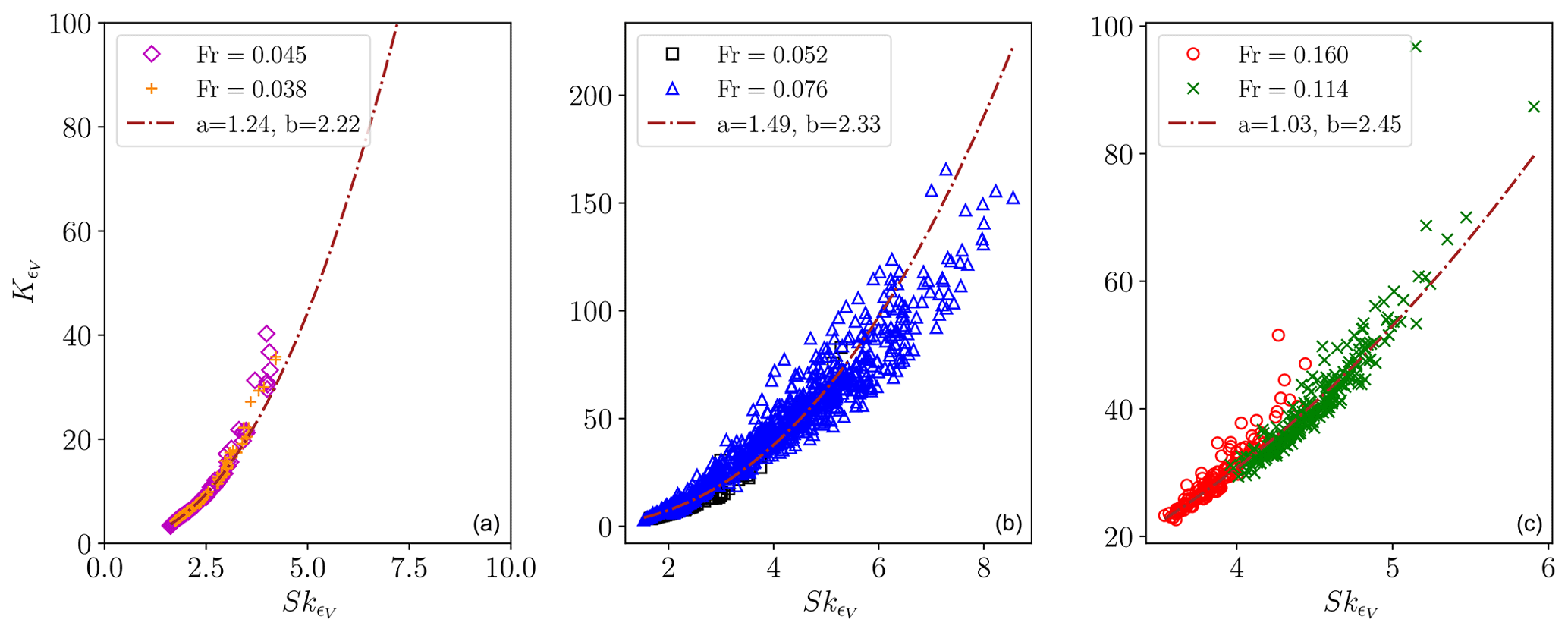
Figure 1 Stratified turbulence: kurtosis-skewness plots for ϵ_v for several Froude numbers (see the insets in which the fit parameters are also given, assuming $K\sim a\cdot S^b$). Note the different scales for S and K, in particular the high K values for the run with Fr≈0.076 (middle).

3.2 Stratified flows in the presence or not of rotation

Now taking into account stable stratification, as is found in the atmosphere and the ocean, we plot in Fig. 1 for several Froude numbers (see the insets) the power law fits for the flatness in terms of $F\left(S\right)\sim S^{{\mathit{\alpha }}_{\mathit{ϵ}}}$ for the kinetic energy dissipation ϵ_v, which is a good indicator of clean-air turbulence (Storer et al., 2019). This leads to an exponent α_ϵ that increases continuously with Fr from ≈2.22 to 2.45 (parameters for the runs are given in Table 1 of PRM2). The highest values of both $S_{{\mathit{ϵ}}_v}$ and $F_{{\mathit{ϵ}}_v}$ are reached for the run with Fr≈0.076, corresponding to the strongest intermittency of the vertical velocity in particular (Feraco et al., 2018; Marino et al., 2022), strong local dissipation, and the associated strong localized shear layers.

When combining rotation and stratification of comparable magnitudes as found in the ocean ($N/f_{\mathrm{0}}\approx \mathrm{5}$), we can observe in Fig. 2 (left) for runs with quasi-geostrophic (QG) forcing (see Table 1 for the PRM2 run specifications) a sharp transition in the exponent of the K(S)∼S^α fits for the buoyancy flux around R_B≈25, corresponding to an average gradient Richardson number of 〈Ri_g〉≈1.5, which is close to that of a KH transition to instability. As noted before, and as opposed to associating the transition with a parabolic law with measurably different coefficients, the transition is now linked to a change in the power law scaling itself, as backed up by the theoretical investigation in Sect. 4, particularly in the context of the generalized She–Lévêque models. This also points to the importance of the occurrence of turbulence at small scales once the Ozmidov scale is larger than the Kolmogorov scale, i.e., ℓ_Oz≥η_K with ${\mathrm{\ell }}_{\mathrm{Oz}}=\sqrt{{\mathit{ϵ}}_V/N^{\mathrm{3}}}$ and ${\mathit{\eta }}_K=[{\mathit{ϵ}}_V/{\mathit{\nu }}^{\mathrm{3}}{]}^{-\mathrm{1}/\mathrm{4}}$. We also give in Fig. 2 the PDFs of the potential energy dissipation ${\mathit{ϵ}}_{\mathit{\theta }}={\mathit{\kappa }}_{\mathrm{0}}\langle |\mathrm{\nabla }\mathit{\theta }{|}^{\mathrm{2}}\rangle$ for the QG runs Q1 (center) and Q8 (right), with buoyancy Reynolds numbers R_B of 3.2 and 385 (see Table 1 in PRM2). The respective fits ($\approx \mathrm{0.1}{\exp }^{-\mathrm{2.7}{\mathit{ϵ}}_{\mathit{\theta }}}$ and $\approx \mathrm{0.0008}{\exp }^{-\mathrm{0.37}{\mathit{ϵ}}_{\mathit{\theta }}}$) are in agreement with the expected increase in small-scale structures and dissipation as R_B grows and a fully turbulent regime is reached.

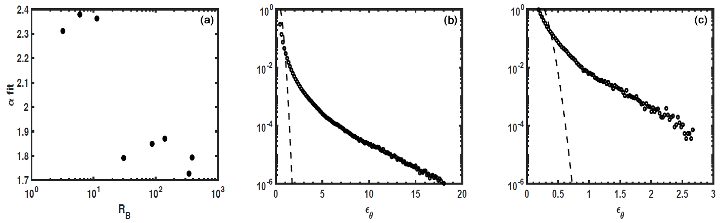
Figure 2 Quasi-geostrophic (QG) turbulence: (a) variation with R_B of the exponent for the K(S)∼S^α scaling of the kinetic energy dissipation, using QG forcing. Note the sharp transition which occurs for R_B≈20 corresponding to 〈Ri_g〉≈1. (b, c) PDFs of potential energy dissipation ϵ_θ for runs with R_B=3 (run Q1, b) and R_B=385 (run Q8, c); see Table 1 and Eq. (3) in PRM2, where PDFs for ϵ_v are given). Dashed lines are for equivalent Gaussians, and lin–log coordinates are used, giving plausibility to the exponential fits (see the text).

3.3 Coupling to a magnetic field in MHD: fast dynamos in the ABC, Roberts, and Taylor–Green flows

The dynamo problem is that of the growth of magnetic fields due to either, at small scales, chaotic streamlines of the velocity, or, at large scales, the kinetic helicity content of the flow, where $H_{\mathrm{V}}=\langle \mathit{u}\cdot \mathit{\omega }\rangle$ (Steenbeck et al., 1966; Moffatt, 1969; Zel'dovich et al., 1983; Brandenburg and Subramanian, 2005) plays an essential role in the solar context in the presence of convection (see, e.g., Ponty et al., 2001). Both the cross-helicity $H_{\mathrm{C}}=\langle \mathit{u}\cdot \mathit{b}\rangle$ (Pouquet et al., 1986; Yokoi, 2013) and the magnetic helicity $H_{\mathrm{M}}=\langle \mathbf{A}\cdot \mathit{b}\rangle$, with $\mathit{b}=\mathrm{\nabla }\times \mathbf{A}$, also play roles, the latter in the nonlinear saturation of the large-scale dynamo associated with an inverse cascade of H_M (Pouquet et al., 1976).² In fact, with sufficient large-scale separation, a dynamo can occur with H_V≡0 overall but with sufficient local fluctuations (Gilbert et al., 1988). The dynamo can also be subcritical because the growing magnetic seed will alter the flow and reduce the turbulence (Ponty et al., 2007; Mannix et al., 2022). The resulting 3-D turbulent system is made up of current and vorticity sheets, rolling up around the local mean magnetic field and with a strong twist of b across the sheet (Mininni et al., 2006; Ponty and Plunian, 2011; Homann et al., 2014); see also Uzdensky et al. (2010), Lazarian et al. (2020), and Oka et al. (2022).

(Quasi)-parabolic K(S) laws in MHD have been found in both laboratory plasmas and the cosmos (Labit et al., 2007; Krommes, 2008; Osmane et al., 2015). Recently, variations of α with parameters were discussed briefly in the context of the classical She–Lévêque (SL) model as found in the fast dynamo context (Ponty et al., 2025), and we expand on these results presently for the generalized SL models (see Eq. (8) analyzed in Sect. 4.1) as well as for higher-order moment ratios.

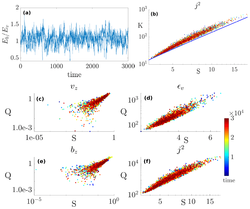
Figure 3 Fast dynamos in MHD for run GOR2 with R_V≈445. (a) $E_{\mathrm{M}}/E_{\mathrm{V}}\left(t\right)$ and (b) K(S) for j². We also give Q(S) for the same run for j² (b), v_z (c), ϵ_v (d), b_z (e), and (f) for j² again, this time in log–log form.

We now give new results for runs already analyzed in part in Ponty et al. (2025) as well as for two new runs with a so-called Roberts flow with helical forcing. These are runs GOR1 and GOR2, with Reynolds numbers of 147 and 445 (and R_λ values of 38 and 66). The runs are performed on 64²×128 and 128²×256 grids. These flows are resolved well (the dissipation scale is more than twice the numerical cutoff according to the Kaneda criteria), and they are run for long times (15 000 and 2000 τ_NL). However, we note that the energy spectra (not shown) are not yet sufficiently developed (see also Ponty and Plunian (2011) for different runs using the Roberts dynamo configuration), although the skewness of j² already reaches high values (above 18).

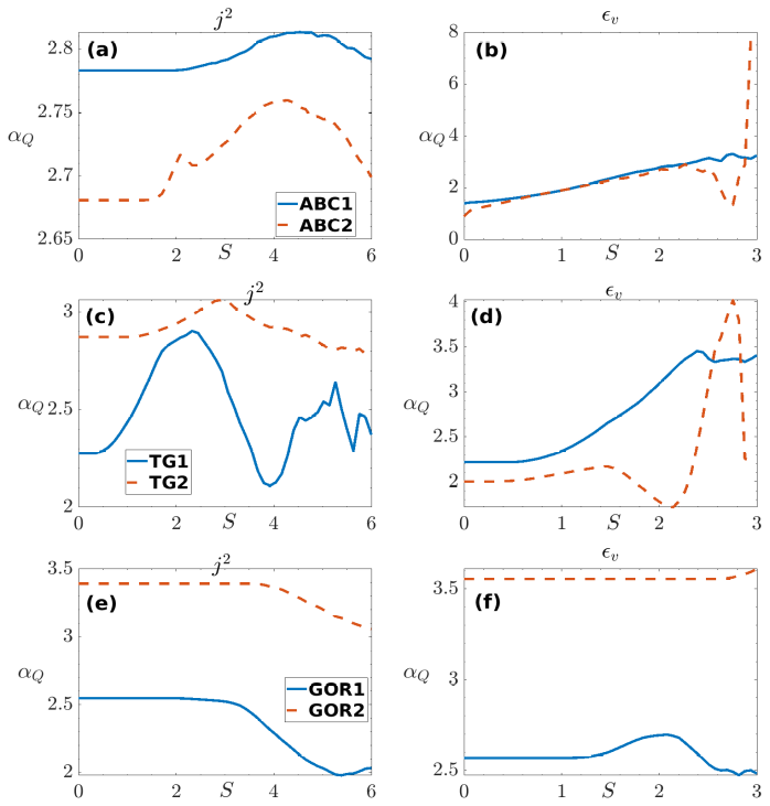
Figure 4 Fast dynamos in MHD. Exponent α for the scaling of $Q=〈\mathit{\delta }{f}^{\mathrm{5}}〉/{〈\mathit{\delta }{f}^{\mathrm{2}}〉}^{\mathrm{5}/\mathrm{2}}$ as a function of the threshold of skewness for the magnetic current (f=j²; a, c, and e) and kinetic energy dissipation (f=ϵ_v; b, d, and f) for runs ABC (a, b), TG (c, d), and GOR (e, f). Note the higher skewness values for j² when compared to ϵ_v and its higher dependency on Reynolds numbers compared to ϵ_v for the ABC and TG runs.

Preliminary results indicate the following. The energy ratio $r_{\mathrm{E}}=E_{\mathrm{M}}/E_{\mathrm{V}}$ approaches equipartition (Fig. 3a), and the K(S) scatterplot for j² for run GOR2 in the plot (Fig. 3b) indicates a rather clear power law, with the blue line following the parabola $K\left(S\right)=\mathrm{3}/\mathrm{2}\left[S^{\mathrm{2}}\mathrm{-}\mathrm{1}\right]$ (see Garcia, 2012). Note that the colors of the dots indicate the time lapse from the onset of the run, in turnover times, from blue (early times) to red (late times on the order of 10⁴; see the color bar to the right). The remaining graphs of Fig. 3 give scatterplots for the normalized fifth-order moment $Q=〈\mathit{\delta }{f}^{\mathrm{5}}〉/{〈\mathit{\delta }{f}^{\mathrm{2}}〉}^{\mathrm{5}/\mathrm{2}}$ for a field f (see Eq. (12) below, with K₅₂≡Q, in an effort to simplify the notation). f is v_z or b_z for Fig. 3c, e, and f is ϵ_v or j² for Fig. 3d, f. In the Q(S) data, power laws emerge in the tails of the kinetic variables and b_z and throughout for j².

The scaling exponent α and constant κ for the normalized fifth-order moments Q are given in Fig. 4 for the ABC (top), TG (middle), and GOR (bottom) runs for j² (left) and ϵ_v (right). They show variations with the forcing function, with Reynolds numbers and the threshold for S used for the plot, together with, possibly, the equipartition ratio r_E. As is the case for the TG and ABC flows, the Reynolds number leads to a difference in scaling for the fit parameters. Thus, runs at higher Reynolds numbers and with several configurations will have to be performed in order to study the scaling of the α and κ parameters for relevant variables, but in the next section we formulate an approach that can elucidate these scaling laws in the framework of three multifractal intermittency models.

4 Theoretical moment scaling using several multifractal intermittency models

4.1 Expression for the kurtosis–skewness scaling exponent, K∼S^α, for both fluids and MHD in the SL framework

We now give a path towards a theoretical formulation for K(S) scaling using a classical intermittency model and several of its extensions, assuming a power law dependency for velocity and magnetic field structure functions δu(r),δb(r) defined as for (scalar) components u and b:

$$\begin{array}{}\text{(6)}& \begin{array}{rl}& \langle \left[u\right(x+r)-u(x){]}^p\rangle \equiv \langle \mathit{\delta }u(r{)}^p\rangle \sim r^{{\mathit{\zeta }}_p^{\left(f\right)}},\\ & \langle \left[b\right(x+r)-b(x){]}^p\rangle \equiv \langle \mathit{\delta }b(r{)}^p\rangle \sim r^{{\mathit{\zeta }}_p^{\left(m\right)}}.\end{array}\end{array}$$

Also assuming power law scaling between kurtosis and skewness for both fluids (f) and MHD (m), we easily obtain

$$\begin{array}{}\text{(7)}& \begin{array}{rl}& K_{\mathrm{f}}\left(S_{\mathrm{f}}\right)\sim S_{\mathrm{f}}^{{\mathit{\alpha }}_{\mathrm{f}}},K_m\left(S_m\right)\sim S_m^{{\mathit{\alpha }}_m},\\ & {\mathit{\alpha }}_{\mathrm{f}}={\displaystyle \frac{{\mathit{\zeta }}_{\mathrm{4}}^{\left(f\right)}-\mathrm{2}{\mathit{\zeta }}_{\mathrm{2}}^{\left(f\right)}}{{\mathit{\zeta }}_{\mathrm{3}}^{\left(f\right)}-\mathrm{3}{\mathit{\zeta }}_{\mathrm{2}}^{\left(f\right)}/\mathrm{2}}},{\mathit{\alpha }}_m={\displaystyle \frac{{\mathit{\zeta }}_{\mathrm{4}}^{\left(m\right)}-\mathrm{2}{\mathit{\zeta }}_{\mathrm{2}}^{\left(m\right)}}{{\mathit{\zeta }}_{\mathrm{3}}^{\left(m\right)}-\mathrm{3}{\mathit{\zeta }}_{\mathrm{2}}^{\left(m\right)}/\mathrm{2}}},\end{array}\end{array}$$

with the functions ${\mathit{\zeta }}_p^{(f,m)}$ depending on the (fluid or MHD) intermittency dynamics or an explicit model.

We now recall the scaling laws derived in the context of the She–Lévêque formulation for fluids (She and Lévêque, 1994) and for MHD as generalized in Politano et al. (1995). These generalized She–Lévêque models, named gslf and gslm for fluids and MHD, depend on two open parameters $\mathrm{0}<x<\mathrm{1}$ and $\mathrm{0}<\mathit{\beta }<\mathrm{1}$, where, in the limit of the non-intermittent case, β→1, whereas β→0 for a monofractal. The anomalous exponents ${\mathit{\zeta }}_p^{\mathrm{gsl}}$ at order p are³

$$\begin{array}{}\text{(8)}& \begin{array}{rl}& {\mathit{\zeta }}_p^{\mathrm{gslf}}={\displaystyle \frac{p(\mathrm{1}-x)}{\mathrm{3}}}+{\displaystyle \frac{x(\mathrm{1}-{\mathit{\beta }}^{p/\mathrm{3}})}{\mathrm{1}-\mathit{\beta }}},\\ & {\mathit{\zeta }}_p^{\mathrm{gslm}}={\displaystyle \frac{p(\mathrm{1}-x)}{\mathrm{4}}}+{\displaystyle \frac{x(\mathrm{1}-{\mathit{\beta }}^{p/\mathrm{4}})}{\mathrm{1}-\mathit{\beta }}}.\end{array}\end{array}$$

We note that x is related to the codimension of the most dissipative structures in the nonlinear system and that β is a measure of the efficiency of energy transfer and dissipation among intermittent structures as the moment order varies. This formulation leads to log-Poisson statistics (see, e.g., She and Lévêque, 1994; Dubrulle, 1994; Frick et al., 1995). A further assumption of the models concerns the scaling of nonlinear transfer in terms of characteristic times of the problem, i.e., the nonlinear eddy turnover time, the wave period (in MHD, the Alfvén wave), and the transfer time of energy to small scales.

The multifractal framework (see Frisch, 1995) allows for a multiplicity of dissipative structures of diverse physical (co)dimensions: vortex and current sheets, flux tubes, current filaments, or bubbles. These result in a non-integer effective β parameter. An extension of the multifractal framework to vectors (velocity field) as opposed to scalars (velocity amplitude) can be found in Schertzer and Tchiguirinskaia (2020). The SL formulation for MHD has been used for example in modeling intermittent nanoflares in connection with solar wind data (Veltri et al., 2005). In the numerical context, it is stressed in Servidio et al. (2011) that a high resolution is needed to properly quantify the properties of local reconnection and current sheets; moreover, reconnection events and the ensuing dissipation are highly local and very varied in amplitude, which is somewhat reminiscent of the multifractality property reviewed in detail in Lovejoy and Schertzer (2013) and Benzi and Toschi (2023).

From Eq. (8), we can compute the general scaling exponents of kurtosis and skewness using Eq. (7). We obtain

$$\begin{array}{}\text{(9)}& \begin{array}{rl}& {\mathit{\alpha }}_{\mathrm{gslf}}={\displaystyle \frac{\mathrm{2}(\mathrm{1}-\mathrm{2}{\mathit{\beta }}^{\mathrm{2}/\mathrm{3}}+{\mathit{\beta }}^{\mathrm{4}/\mathrm{3}})}{\mathrm{1}+\mathrm{2}\mathit{\beta }-\mathrm{3}{\mathit{\beta }}^{\mathrm{2}/\mathrm{3}}}};\\ & {\mathit{\alpha }}_{\mathrm{gslm}}={\displaystyle \frac{\mathrm{2}(\mathrm{1}-\mathrm{2}{\mathit{\beta }}^{\mathrm{1}/\mathrm{2}}+\mathit{\beta })}{\mathrm{1}+\mathrm{2}{\mathit{\beta }}^{\mathrm{3}/\mathrm{4}}-\mathrm{3}{\mathit{\beta }}^{\mathrm{1}/\mathrm{2}}}},\mathit{\beta }\ne \mathrm{1}.\end{array}\end{array}$$

Note that, interestingly, both the α_gslf and α_gslm exponents are independent of x, the fractal codimension of the most dissipative structures. It is also easy to see, again for both fluids and MHD, that the limit for β→0 is α→2. In other words, a parabolic law is reached when the most dissipative structure dominates the small-scale dynamics irrespective of its geometrical (co)dimension, likely at high R_V, high R_M, and 〈Ri_g〉≈1 (see Eq. 3). We note that a similar result from the computation of the α exponent could be written in the context of the model developed in Horbury and Balogh (1997). We also note however that, in the shell models examined in Frick et al. (1995), β never reaches this low limit. Another point concerns the fact that the variation of α could reflect the dependence on the form of the second invariant in the shell models, which is akin to helicity (Frick et al., 1995; Kadanoff et al., 1995). This may point to a limitation of such models when restricted to nearest-neighbor interactions or with different sets of invariants, restrictions that cannot encompass by construction the highly nonlocal (in scale) interactions leading to anomalous dissipation. Thus, this point will need further investigations.

4.2 The standard choice of parameters for the SL models for fluids and MHD

The standard case for the classical fluid SL model is obtained for $x=\mathrm{2}/\mathrm{3},\mathit{\beta }=\mathrm{2}/\mathrm{3}$ and is associated with vortex filaments, whereas in the MHD case with wave–vortex interactions and current sheets, the standard parameters become $x=\mathrm{1}/\mathrm{2},\mathit{\beta }=\mathrm{1}/\mathrm{2}$ (Grauer et al., 1994; Politano and Pouquet, 1995). This yields, respectively, for the K(S)∼S^α for fluids (sslf) and MHD (sslm),

$$\begin{array}{}\text{(10)}& \begin{array}{rl}& {\mathit{\zeta }}_p^{\mathrm{sslf}}={\displaystyle \frac{p}{\mathrm{9}}}+\mathrm{2}\left[\mathrm{1}-{\left({\displaystyle \frac{\mathrm{2}}{\mathrm{3}}}\right)}^{p/\mathrm{3}}\right],{\mathit{\alpha }}_{\mathrm{sslf}}\approx \mathrm{2.56};\\ & {\mathit{\zeta }}_p^{\mathrm{sslm}}={\displaystyle \frac{p}{\mathrm{8}}}+\mathrm{1}-{\displaystyle \frac{\mathrm{1}}{{\mathrm{2}}^{p/\mathrm{4}}}},{\mathit{\alpha }}_{\mathrm{sslm}}\approx \mathrm{2.53}.\end{array}\end{array}$$

These α values for the standard SL models are also given in Ponty et al. (2025)⁴.

All α values are close except for extreme cases (β at its limits), in part because the values of the anomalous exponents for structure functions for fluids are anchored at ζ₃≡1. For θ,v, and b, there are more complex constraints since they involve cross-correlations between fields at third order (Yaglom, 1949; Antonia et al., 1997; Politano and Pouquet, 1998) and also because the analytical expressions for α lead to a small fractional power of β, and we are at relatively low orders of the structure functions. In fact, an extension of the SL theory to the intermittency of the passive scalar θ in the fluid case can be found in Lévêque et al. (1999). We can then derive the expression $K_{F_{\mathit{\theta }}}\sim S_{F_{\mathit{\theta }}}^{{\mathit{\alpha }}_{\mathit{\theta }}}$ in the framework of that model. Here, the scalar flux F_θ is defined as $F_{\mathit{\theta }}(r{)}^{\left(p\right)}:=\langle |\mathit{\delta }u\left(r\right)\mathit{\delta }\mathit{\theta }(r{)}^{\mathrm{2}}{|}^{p/\mathrm{3}}\rangle \sim \langle |\mathit{\delta }u\left(r\right)\mathit{\delta }\mathit{\theta }(r{)}^{\mathrm{2}}{|}^{{\mathit{\zeta }}_p}\rangle$, an expression using the flux arising from the aforementioned exact law for the conservation of scalar energy derived in Yaglom (1949). With the numerical values given in Lévêque et al. (1999), we find ${\mathit{\alpha }}_{\mathit{\theta }}^E\approx \mathrm{2.61}$ using anomalous exponents stemming from experiments, ${\mathit{\alpha }}_{\mathit{\theta }}^D\approx \mathrm{2.38}$ for DNS, and ${\mathit{\alpha }}_{\mathit{\theta }}^T\approx \mathrm{2.44}$ using the theory developed in that paper. This shows again the sensitivity of these power laws to the accuracy of the data.

4.3 Generalized scaling for higher-order normalized structure functions in the framework of the She–Lévêque models

Let us now rewrite the generalized SL models for fluid and MHD slightly differently, with (as before) $\mathrm{0}<\mathit{\beta }<\mathrm{1}$ and $\mathrm{0}<x<\mathrm{1}$:

$$\begin{array}{}\text{(11)}& \begin{array}{rl}& \mathrm{3}(\mathrm{1}-\mathit{\beta }){\mathit{\zeta }}_p^{\mathrm{gslf}}=x\left[\mathrm{3}\right(\mathrm{1}-{\mathit{\beta }}^{p/\mathrm{3}})+p(\mathit{\beta }-\mathrm{1}\left)\right]+p(\mathrm{1}-\mathit{\beta }),\\ & \mathrm{4}(\mathrm{1}-\mathit{\beta }){\mathit{\zeta }}_p^{\mathrm{gslm}}=x\left[\mathrm{4}\right(\mathrm{1}-{\mathit{\beta }}^{p/\mathrm{4}})+p(\mathit{\beta }-\mathrm{1}\left)\right]+p(\mathrm{1}-\mathit{\beta }).\end{array}\end{array}$$

We now compute the scaling of a generalized adimensionalized structure function versus another one, provided they exist, writing

$$\begin{array}{}\text{(12)}& \begin{array}{rl}& K_{pq}={\displaystyle \frac{\langle \mathit{\delta }{u}^p\rangle }{\langle \mathit{\delta }{u}^q{\rangle }^{p/q}}},K_{rs}={\displaystyle \frac{\langle \mathit{\delta }{u}^r\rangle }{\langle \mathit{\delta }{u}^s{\rangle }^{r/s}}},\\ & K_{pq}=f\left(K_{rs}\right)=K_{rs}^{{\mathit{\alpha }}_{\mathit{\sigma }}},\mathit{\sigma }=[pr/qs],\\ & {\mathit{\alpha }}_{\mathit{\sigma }}={\displaystyle \frac{{\mathit{\zeta }}_p-[p/q]{\mathit{\zeta }}_q}{{\mathit{\zeta }}_r-[r/s]{\mathit{\zeta }}_s}},\end{array}\end{array}$$

with $\mathit{\sigma }\in {\mathbb{N}}^{+},p>max[q,r],r>s$. In Sect. 4.1, we considered the case K=S^α or, in the present notation, $K_{\mathrm{42}}=K_{\mathrm{32}}^{{\mathit{\alpha }}_{\mathrm{43}/\mathrm{22}}}$, with $p=\mathrm{4},q=\mathrm{2}=s$, and r=3. After a slightly cumbersome but straightforward computation, one finds again that α_σ is independent of x, the codimension of dissipative structures, for all values of the indices encapsulated in σ; one finds, specifically, that

$$\begin{array}{}\text{(13)}& \begin{array}{rl}& {\mathit{\alpha }}_{\mathit{\sigma }}^{\left(\mathrm{gslf}\right)}={\displaystyle \frac{s}{q}}\left[{\displaystyle \frac{q(\mathrm{1}-{\mathit{\beta }}^{p/\mathrm{3}})-p(\mathrm{1}-{\mathit{\beta }}^{q/\mathrm{3}})}{s(\mathrm{1}-{\mathit{\beta }}^{r/\mathrm{3}})-r(\mathrm{1}-{\mathit{\beta }}^{s/\mathrm{3}})}}\right],\\ & {\mathit{\alpha }}_{\mathit{\sigma }}^{\left(\mathrm{gslm}\right)}={\displaystyle \frac{s}{q}}\left[{\displaystyle \frac{q(\mathrm{1}-{\mathit{\beta }}^{p/\mathrm{4}})-p(\mathrm{1}-{\mathit{\beta }}^{q/\mathrm{4}})}{s(\mathrm{1}-{\mathit{\beta }}^{r/\mathrm{4}})-r(\mathrm{1}-{\mathit{\beta }}^{s/\mathrm{4}})}}\right].\end{array}\end{array}$$

In the case of extreme intermittency with β→0, we also have, for fluids, MHD, and s≠r, as stated before,

$$\begin{array}{}\text{(14)}& \mathit{\beta }\to \mathrm{0},{\mathit{\alpha }}_{pr/qs}^{\left(\mathrm{gslf}\right),\left(\mathrm{gslm}\right)}\to {\displaystyle \frac{s(p-q)}{q(r-s)}}.\end{array}$$

This formula simplifies, for q=s (same normalization of moments), into $[p-q]/[r-q]$ and gives a parabolic scaling for $p+q=\mathrm{2}r$. Thus, when choosing for the normalization the second-order energy moment ($q=s=\mathrm{2}$), we have a parabolic scaling for $\mathrm{2}r=p+\mathrm{2}$. Similarly, for a normalization by the skewness, $q=s=\mathrm{3}$, we again obtain a parabola for $\mathrm{2}r=p+\mathrm{3}$. These parabolic solutions for β→0 are directly linked to the algebraic and hierarchical formulations of the SL models.

Finally, let us take two specific examples: Q(S) with $p=\mathrm{5},q=s=\mathrm{2}$, and r=3 and H₆(S) with $p=\mathrm{6},q=s=\mathrm{2}$, and r=3 (sometimes called hyper-flatness). The first example for Q(S) is also discussed in Sardeshmukh and Sura (2009). We find in the standard case ($\mathit{\beta }=\mathrm{2}/\mathrm{3}$ for fluids and $\mathit{\beta }=\mathrm{1}/\mathrm{2}$ for MHD) the scalings ${\mathit{\alpha }}_{\mathrm{53}/\mathrm{22}}^{\mathrm{sslf}}\approx \mathrm{4.6}$ and ${\mathit{\alpha }}_{\mathrm{53}/\mathrm{22}}^{\mathrm{sslm}}\approx \mathrm{4.5}$, whereas the numerical estimate for the ABC runs gives a maximum of Q≈3.5. When $\mathit{\beta }\to \mathrm{0},{\mathit{\alpha }}_{\mathrm{53}/\mathrm{22}}^{\mathit{\beta }\to \mathrm{0}}\to \mathrm{3}$, a value advocated in Sardeshmukh and Sura (2009) for this Q(S) scaling for both vorticity and potential height using a linear stochastically forced Langevin equation model for climate dynamics with correlated additive and multiplicative noise (see also Sect. 5.1 below). To give a second and final example, for H₆ in the standard case again, we have ${\mathit{\alpha }}_{\mathrm{63}/\mathrm{22}}^{\mathrm{sslf}}\approx \mathrm{7.1}$ and ${\mathit{\alpha }}_{\mathrm{63}/\mathrm{22}}^{\mathrm{sslm}}\approx \mathrm{6.8}$, and when $\mathit{\beta }\to \mathrm{0},{\mathit{\alpha }}_{\mathrm{63}/\mathrm{22}}^{\mathit{\beta }\to \mathrm{0}}\to \mathrm{4}$, whereas the numerical value we find for the ABC runs is close to 3.7. The discrepancy with the data in Fig. 4 is thus large. In this context, a study in terms of variation in Reynolds numbers will be informative, but one may have to investigate the MHD turbulence case in 2-D or so-called “2.5-D” (two space variations and three components of the fields) to reach substantially higher R_V and R_M values.

4.4 K∼S^α scaling for the Yakhot intermittency model

One can use other models of structure function scaling in turbulent flows. For example, a model of intermittency in fluid turbulence by Yakhot (2006) (hereafter model Y) yields the scaling

$$\begin{array}{}\text{(15)}& \begin{array}{rl}& {\mathit{\zeta }}_{\mathrm{2}p}^{\left(Y\right)}={\displaystyle \frac{\mathrm{2}(\mathrm{1}+\mathrm{3}{\mathit{\beta }}_y)p}{\mathrm{3}(\mathrm{1}+\mathrm{2}p{\mathit{\beta }}_y)}},{\mathit{\zeta }}_{\mathrm{3}}^{\left(Y\right)}=\mathrm{1}\forall {\mathit{\beta }}_y,\\ & q=\mathrm{2}p,{\mathit{\zeta }}_q^{\left(Y\right)}={\displaystyle \frac{q(\mathrm{1}+\mathrm{3}{\mathit{\beta }}_y)}{\mathrm{3}(\mathrm{1}+q{\mathit{\beta }}_y)}}.\end{array}\end{array}$$

The model comes from evaluating, in terms of perturbation, the corrections to 2-D turbulence when close to a critical dimension at which the energy cascade reverses its direction to small scales. One can verify that β_y=0 gives a ${\mathit{\zeta }}_p=p/\mathrm{3}$ standard scaling. We immediately get α_y≈2.56 for the relationship $K\sim S^{{\mathit{\alpha }}_y}$ when choosing the value β_y≈0.05 for the open parameter, which is close to that given by the experiments. See also Nickelsen (2017) and Friedrich and Grauer (2020) for recent analyses of this and other models⁵. The anomalous ζ_p exponents themselves (see Fig. 1 in Friedrich and Grauer, 2020) do not differ by much from model to model, especially at a relatively low order. However, in view of the sensitivity of α to the evaluation of the anomalous exponents, α scaling in an empirical K(S) law may prove a valuable tool in order to distinguish between different intermittency modeling and small-scale parameterizations in general, which is somewhat better than with the ζ_p values themselves, given sufficiently resolved data leading to precise fits to the quasi-parabolic power law behavior for long runs in terms of turnover times.

In conclusion, if the change in K(S) scaling with the Reynolds number is not known and is difficult to evaluate experimentally or numerically, the data are sufficient to see that such scalings will be observed at high R_V values. Indeed, this can be expected in the framework of random multiplicative systems (see Benzi and Toschi (2023) for a recent introduction). We also recall here that a parabolic law can be justified on several grounds. First, as stated earlier, one can write a Taylor expansion for K(S) for a quasi-Gaussian PDF and note that K≥0. Another reason for observing a K(S) parabolic law relies on the existence of Cauchy–Schwarz relationships (and their generalizations) between the third- and fourth-order moments of a stochastic variable f, i.e., $S_{\mathrm{f}}^{\mathrm{2}}\le K_{\mathrm{f}}+\mathrm{3}$, with a tightening of the inequality for a unimodal PDF, i.e., $S_{\mathrm{f}}^{\mathrm{2}}\le K_{\mathrm{f}}+\mathrm{186}/\mathrm{125}$, for a finite fourth-order moment (Klaassen et al., 2000). We also note that Beta distributions are advocated in Labit et al. (2007) for the intermittency of density fluctuations in drift-exchange turbulence in plasmas, in particular because they admit both positive and negative skewnesses, as observed in many instances, e.g., the fast dynamo (Ponty et al., 2025). These K(S) relations also provide useful bounds for the data.

5 Other approaches for quasi-parabolic scaling beyond the GSL and Y models

5.1 Linear and nonlinear Langevin models

Langevin equations have long been written in the context of turbulent flows, e.g., in order to take into account the nonlocality of mode interactions leading to intermittency, modeling as such the separation of spatial and temporal scales (Nazarenko et al., 2000a; Laval et al., 2003). Indeed, dissipative and intermittent structures such as shear layers or current sheets are multiscale, spanning a range from the integral scale characteristic of their length to the dissipative scale defined by viscosity or resistivity, e.g., the Kolmogorov scale η_K for NS, providing one possibility for intermittency to be found at both large and small scales. We note however that, in a multifractal framework such as in SL models, there is a range of dissipative scales also corresponding to a plage of spectral indices. This provides a justification for the application of a Langevin framework, where the original nonlinearities of the primitive equations are modeled through fast-evolving additive and multiplicative stochastic noise. It is shown in Wan et al. (2012) that the kurtosis of the magnetic field filtered at the dissipation scale and smaller increases sharply and significantly in high-resolution 2-D DNS and in ACE and Cluster solar wind data. Recent observations in the heliosphere analyzing data from the Parker Solar Probe confirm the importance of such nonlocal interactions in the case of so-called imbalanced MHD turbulence with ${\mathbf{z}}^{\pm }=\mathit{v}\pm \mathit{b}$ of unequal amplitudes (Yang et al., 2023), which is an imbalance enhanced by the quasi-absence of collisions (Miloshevich et al., 2021).

One can write a stochastic Langevin equation for a fluctuating field $\stackrel{\mathrm{̃}}{c}$ in terms of $D_t\stackrel{\mathrm{̃}}{c}=-({\overline{\mathit{\lambda }}}_k+{\mathit{\lambda }}_k^{\prime })\stackrel{\mathrm{̃}}{c}+{\stackrel{\mathrm{̃}}{\mathit{\zeta }}}_k$, where $[{\overline{\mathit{\lambda }}}_k,{\mathit{\lambda }}_k^{\prime }]$ represents large-scale and fluctuating small-scale velocities stretching the magnetic field lines in the kinematic phase and ${\stackrel{\mathrm{̃}}{\mathit{\zeta }}}_k$ is an additive noise due to (plausible) rapid small-scale fluctuations. The essential features in the development by Sura and Sardeshmukh (2008) for climate can thus be reproduced in the MHD case; this will likely lead to the same conclusion of parabolic behavior. The large-scale velocity and induction are constrained by divergence-free conditions, by Galilean invariance for the velocity, and perhaps even more importantly by existing so-called exact laws⁶. Such laws involve third-order cross-correlations of u and b (see Marino and Sorriso-Valvo (2023) for a recent review), whereas the fourth-order moments do not have such constraints for quadratically nonlinear equations. A nonzero energy dissipation rate (a plausible conjecture) thus implies non-Gaussianity (S≠0 and K≠0). A Langevin equation developed in the kinematic dynamo regime can be amended to model the back reaction of the Lorenz force, as discussed briefly in Ponty et al. (2025). We finally note that, starting from well-resolved data, one can reconstruct a Langevin equation model of the observed stochastic process (Friedrich et al., 2011; Rinn et al., 2016). This may prove instructive, in particular if different models were to emerge for different regimes or dynamo types.

5.2 The nonlinear Langevin approach for the dynamo regime

Several Langevin approaches in MHD have been derived in the nonlinear case (see Zwanzig, 1973, for an early study for fluids). For example, a sub-diffusive behavior was shown by Balescu et al. (1994), from first principles, in the context of a stochastic magnetic field. One can also choose to add a cubic term to the induction equation (cubic so that the symmetry of the axial magnetic field is preserved) in order to mimic the effect the Lorentz force has on the velocity (see, e.g., Boldyrev, 2001; Leprovost and Dubrulle, 2005), in particular for large magnetic Prandtl numbers. On the other hand, it was shown in Nazarenko et al. (2000b) that, in the case of the fast dynamo, the feedback of the growing induction is through the creation of counter-rotating vortices, a point not included in a saturation involving only the magnetic field equation. One can also consider the role of Alfvén waves in the nonlinear regime by introducing an oscillatory term into a linear Langevin equation (Bandyopadhyay et al., 2018). Note that, in a Langevin equation, in a sense one is getting rid of the closure problem for turbulent motions since it is linear, with the complex nonlinear small-scale dynamics bundled up in a rapid stochastic forcing with an assumption of (mostly) local interactions between these fast motions.

5.3 Self-organized criticality and the $\mathrm{1}/f$ law as other possible frameworks for intermittent quasi-parabolic scaling

Self-organized criticality (SOC) has been introduced in the context of sandpile systems and their avalanching properties (Bak et al., 1987), such as when modeling solar flares (Lu and Hamilton, 1991); see also Bramwell et al. (2000), Chapman and Watkins (2001), Osman et al. (2014), Watkins et al. (2016), and Balasis et al. (2023) for recent discussions. It can be seen as a system with slow driving and fast relaxation, leading to power law scaling of spatiotemporal dissipative avalanches. In the context of DNS in 3-D MHD, Uritsky et al. (2010) identified SOC in the dissipative range of decaying runs (i.e., with a local critical Reynolds number of order unity). However, SOC was not found in the inertial range, a fact that was interpreted as SOC properties propagating from the dissipative to inertial ranges, with merging of current structures. Indeed, the dissipative features of turbulent flows are multiscale, spanning from the energy-containing range to the dissipative one, such as in vortex filaments and current sheets (see Watkins et al., 2016, for a comparative study of the definitions of SOC behavior). The critical state is that in which the source (the energy cascade at a fixed rate) and sink (the dissipation at a fixed rate through, e.g., eddy viscosity) balance out, as they do on average. Note that Smyth et al. (2019) identified SOC in rotating stratified flows with the Richardson number (governing shear instabilities such as KH), being the critical parameter (see also Fig. 2a). The nonlinear interactions in the inertial range are conservative, and dissipation sets in through nonlocal interactions between energy-containing eddies and dissipative ones, leading these interactions to be described by SOC together with $\mathrm{1}/f$ noise (Vespignani and Zapperi, 1998). As shown in Dmitruk and Matthaeus (2007), this leads to an emphasis on the dynamics of the largest modes and their interactions with the early dissipative range, where intermittency is strongest (Kraichnan, 1967b; Chen et al., 1993). Also, the sharp variations of the flow and field due to the nonlinearities of the primitive equations can be treated as a stochastic force using re-normalization group techniques, which is again reminiscent of a Langevin approach (Materassi and Consolini, 2008). In all of these studies, nonlinear shear instabilities appear central to the interrelated small-scale and large-scale behavior of the stochastic turbulent flows.

6 Conclusions and perspectives

We have analyzed in this paper the relative behavior of normalized moments of the velocity, magnetic field, and temperature fluctuations in a variety of contexts, and we have given a rationale for casting these results in the mold of classical intermittency models for fluid and MHD turbulence, models which provide a natural framework for such relative scalings. The variability of the scaling is linked to the details of the dissipative structures and their relative intensities. The ubiquity of a quasi-parabolic K(S)∼S^α law could be interpreted as it having no specific physical meaning; on the other hand, it may be pointing to a universality of intermittency in turbulent flows. We also note that the power law exponent α is independent of the (co)dimension of the dissipative structures. The abrupt transition in α scaling for the rotating stratified case when shear instabilities arise (see Fig. 2) is indicative of underlying dynamics where the development of turbulence, as measured by the Ozmidov scale becoming larger than the dissipative scale in that case, plays a dynamical role (Pouquet et al., 2023). In MHD, one issue absent from the present analysis is the incorporation of the potential effect of helical structures (with nonzero kinetic helicity, magnetic helicity, and/or cross-helicity) into the K(S) scaling. It is known from multiple studies that helicity plays a central role in large-scale dynamos (see Brandenburg and Subramanian, 2005) and that its incorporation into closures of turbulence leads to better modeling of these flows (Yokoi, 2013).

The multifractality of the She–Lévêque model is measured through the β parameter. As β→0, the intermittency of the flow is carried by one single structure and the flow becomes, in that extreme case, monofractal. In such a limit, α→2 (see Eq. 9), so that a strict parabolic behavior for K(S), in the framework of such models, is linked to monofractality. We also note that the PDFs of the potential energy dissipation rate computed in this paper for quasi-geostrophic flows have exponential tails (see Fig. 2), with lesser decay as the Reynolds number increases. For the so-called α-stable processes, the scaling exponents of normalized moments of the multifractal dynamics can be computed, and this can be associated with (in some cases unbounded) singularities; see Serinaldi (2010) in the context of rainfall. Furthermore, such multifractal analysis could give information on the latitudinal dependency of data and unravel different regimes in the dynamics of the atmosphere, weather, macroweather, and climate (Lovejoy, 2018).

In this context, a standard analysis of anomalous exponents of temporal structure functions (as opposed to spatial ones) in the various data sets presented herein will be of great interest and is planned for future work. Moreover, temporal moment analysis allows one to sort out shorter and longer timescales in time series of nonlinear phenomena and their statistics, such as in climate data (Franzke et al., 2020). Finally, multifractal analysis, through the computation of anomalous scaling exponents of order p and of an evaluation of their limit as the order p→∞ (see, e.g., Pierrehumbert, 1996), can lead to useful characterizations of turbulent structures, e.g., in kilometer-sized clouds (Freischem et al., 2024).

In order to pursue the investigation of K(S) laws of turbulence at higher Taylor–Reynolds numbers, one can implement hyperviscosity algorithms or else use models which, because they are significantly less costly numerically, will allow for longer statistics at substantially higher R_V values. Such approaches are numerous. One can think of shell models retaining only one mode per field per wavenumber shell and only nearest-neighbor interactions as developed for MHD in Gloaguen et al. (1985) (see Plunian et al., 2013, for a review). One can also simplify the dynamics by lowering the space dimension, as for the 1-D, 2-D, and 2.5-D cases (see, e.g., Thomas, 1970; Hada, 1993; Laveder et al., 2013; Merrifield et al., 2007; Servidio et al., 2011). Numerical adaptation, preferably spectral when dealing with L_∞ norms as for extreme intermittent events (see Ng et al., 2008), various large-eddy simulations (Sagaut and Cambon, 2008), or the so-called α model (Holm et al., 1998) used for example in the framework of oceanic dynamics (Pietarila Graham and Ringler, 2013) or also analyzed in MHD (Montgomery and Pouquet, 2002), will be similarly useful. These methods will allow for disentanglement between Reynolds numbers and intermittency effects, the consequences of the presence or not of helicity linked to vortex filaments and the dynamo, and equipartition or not of kinetic, potential, or magnetic energy.

One further important issue will be incorporating the role of anisotropy, which can affect scaling properties and interpretations of the intermittency, as shown in the context of the atmosphere in Lovejoy et al. (2001) or MHD in Schekochihin (2022). Finally, it was noted in Yeung et al. (2018) that the grid resolution, Courant number, and machine precision all affect the estimate of the overall enstrophy. Furthermore, the scaling for the strongest gradients becomes linear in R_λ at high values of R_λ, with intermittent structures found at scales smaller than the Kolmogorov scale η_K (Buaria et al., 2019), confirming the existence of intermittency beyond η_K. In addition, in Buaria and Pumir (2025), a relative scaling of moments of the velocity gradient tensor (restricted to longitudinal components) is analyzed using high R_λ numerical and experimental fluid turbulence data. These authors show the possibility of a universal scaling behavior of relative moments where R_λ disappears, and with explicit data on H₆. This type of analysis is not performed here for lack of a sufficiently large Reynolds number and the ensuing lack of sufficiently intense localized dissipation, but a study of intermittent structures in MHD at a substantially higher Reynolds number is planned for the future.