Improving ensemble data assimilation through Probit-space Ensemble Size Expansion for Gaussian Copulas (PESE-GC)

Small forecast ensemble sizes (< 100) are common in the ensemble data assimilation (EnsDA) component of geophysical forecast systems, thus limiting the error-constraining power of EnsDA. This study proposes an efficient and embarrassingly parallel method to generate additional ensemble members: the Probit-space Ensemble Size Expansion for Gaussian Copulas (PESE-GC; “peace gee see”). Such members are called “virtual members”. PESE-GC utilizes the users' knowledge of the marginal distributions of forecast model variables. Virtual members can be generated from any (potentially non-Gaussian) multivariate forecast distribution that has a Gaussian copula. PESE-GC's impact on EnsDA is evaluated using the 40-variable Lorenz 1996 model, several EnsDA algorithms, several observation operators, a range of EnsDA cycling intervals, and a range of forecast ensemble sizes. Significant improvements to EnsDA (p<0.01) are observed when either (1) the forecast ensemble size is small (≤20 members), (2) the user selects marginal distributions that improve the forecast model variable statistics, and/or (3) the rank histogram filter is used with non-parametric priors in high-forecast-spread situations. These results motivate development and testing of PESE-GC for EnsDA with high-order geophysical models.

1 Introduction

Geophysical forecast models are often computationally expensive to run. As a result, geophysical ensemble data assimilation (EnsDA) typically uses <100 forecast ensemble members. Such small forecast ensemble sizes result in sampling errors that degrade the performance of EnsDA. As such, low-cost methods that introduce additional ensemble members (henceforth virtual members) to the original forecast members (henceforth forecast members) have the potential to improve EnsDA.

Several types of ensemble expansion methods have been proposed in the literature, all of which have strengths and weaknesses. The first type is random draws from climatology (Castruccio et al., 2020; El Gharamti, 2020; Lei et al., 2021). Though computationally efficient, this type of ensemble expansion method cannot generate members with flow-dependent ensemble statistics.

An alternative type of ensemble expansion method is to aggregate forecast ensemble members across time (Xu et al., 2008; Yuan et al., 2009; Huang and Wang, 2018; Gasperoni et al., 2022). Though this type of method efficiently produces members with flow-dependent statistics, the number of virtual members created is limited (Huang and Wang, 2018; Gasperoni et al., 2022).

A third type of ensemble expansion method is to search a historical catalog for forecast states similar to the current forecast or observations (Van den Dool, 1994; Tippett and Delsole, 2013; Monache et al., 2013; Wan and Van Der Merwe, 2000; Grooms, 2021; Sun et al., 2022). The virtual members resulting from this search have flow-dependent statistics. Though such methods are historically expensive to employ, ongoing research may render them affordable in the near future (e.g., Sun et al., 2024).

Ensemble modulation (Bishop and Hodyss, 2009, 2011; Bishop et al., 2017; Kotsuki and Bishop, 2022; Wang et al., 2021) is the fourth type of the ensemble expansion method. Such methods expand ensembles by combining a localization matrix with the original ensembles' perturbations (see Bishop and Hodyss, 2009, for details). Though the expanded ensemble possesses the same mean and variance as the original ensemble, the expanded ensemble's kurtosis can be much larger than the original ensemble's (see the Supplement). In other words, the expanded ensemble's kurtosis is likely biased. If nonlinear observation operators are applied to the expanded ensemble, this kurtosis bias will result in biased expanded ensemble observation statistics (Craig Bishop and Lili Lei, personal communication, 2023).

The shortcomings of existing ensemble expansion methods motivate the development of a new ensemble expansion method. This study proposes a new ensemble expansion method that explicitly utilizes the users' knowledge of prior marginals, the Probit-space Ensemble Size Expansion for Gaussian Copulas (PESE-GC). PESE-GC constructs virtual members using a generalization of the efficient and scalable Gaussian resampling algorithm of Chan et al. (2020) (henceforth the CAC2020 algorithm). Unlike existing methods, PESE-GC efficiently and scalably generates an unlimited number of virtual members with flow-dependent statistics. Furthermore, the PESE-GC produces virtual members that are consistent with user-specified prior marginals and handles multivariate Gaussian distributions and many multivariate non-Gaussian distributions. PESE-GC is applied before running any observation operators for EnsDA, and the analyzed virtual members are discarded before generating the next forecast ensemble (see Fig. 1). To the author's knowledge, no other ensemble expansion methods simultaneously possesses the same efficiency, scalability, generality, and flow-dependency as PESE-GC.

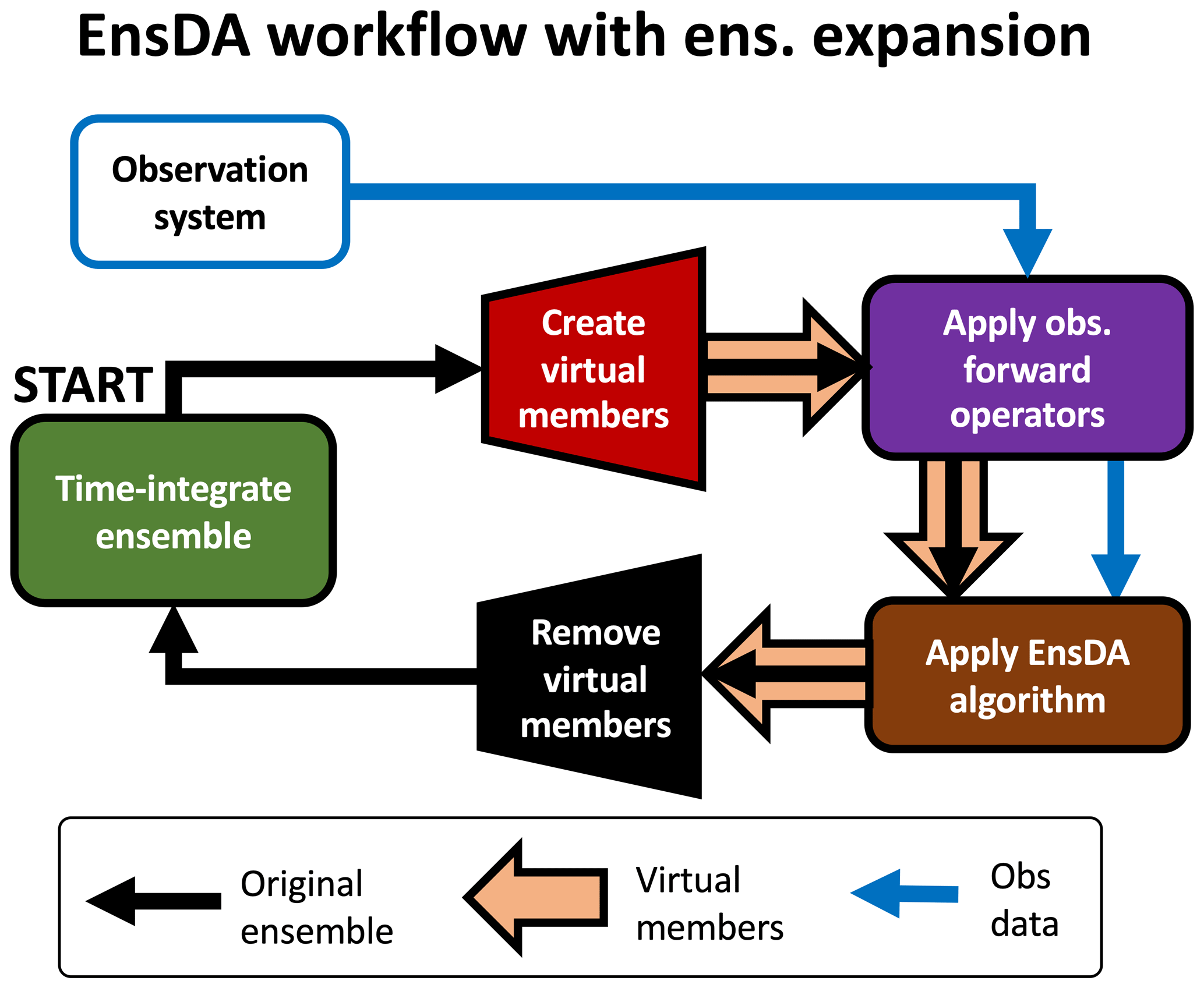
Figure 1 An illustration of how PESE-GC can be integrated into a typical EnsDA cyclic workflow. This workflow is meant to be read starting from the green box labeled START. The arrows indicate the movement of various kinds of information (see legend). For example, the fat orange arrows indicate that the virtual members are created by PESE-GC (red polygon), passed to the observation operators (rounded purple box), passed to the EnsDA algorithm (rounded brown box), and then removed before applying the forecast model (black polygon). Obs stands for observation and ens stands for ensemble.

The remainder of this publication is divided into five sections. Section 2 discusses the formulation of PESE-GC and its computational complexity and scalability. PESE-GC's impacts on EnsDA are discussed and illustrated in Sect. 3. PESE-GC is then tested with EnsDA using the Lorenz 1996 (L96) model in Sect. 4. Section 5 discusses an important caveat and the computational economy of the PESE-GC method. This publication then ends with Sect. 6 and a summary and a discussion of avenues for future research therein.

2 Formulation of PESE-GC

This section begins with reviewing the CAC2020 algorithm. The CAC2020 algorithm is then generalized to handle arbitrary piecewise continuous marginal distributions (i.e., one-dimensional distributions) using probit probability integral (PPI) transforms. Finally, the computational complexity and scalability of PESE-GC is discussed.

2.1 The CAC2020 algorithm

The CAC2020 algorithm constructs Gaussian-distributed virtual members through linear combinations of the forecast ensemble perturbations. The resulting expanded ensemble has the same mean state and covariance matrix as the forecast ensemble. The CAC2020 algorithm was first formulated by Chan et al. (2020), and a more comprehensive derivation is presented in Chap. 7 of Chan (2022).

To write down the CAC2020 algorithm, a notation similar to Ide et al. (1997) is used. Suppose x is an N_x-dimensional column vector representing a forecast model state, and $\left\{{\mathit{x}}_{\mathrm{1}}^{\mathrm{f}},{\mathit{x}}_{\mathrm{2}}^{\mathrm{f}}\mathrm{\dots }{\mathit{x}}_{N_{\mathrm{E}}}^{\mathrm{f}}\right\}$ represents an ensemble of N_E forecast model states.

$$\begin{array}{}\text{(1)}& {\mathit{x}}_n^{{\mathrm{f}}^{\prime }}\equiv {\mathit{x}}_n^{\mathrm{f}}-{\displaystyle \frac{\mathrm{1}}{N_{\mathrm{E}}}}\sum _{n^{\prime }=\mathrm{1}}^{N_{\mathrm{E}}}{\mathit{x}}_{n^{\prime }}^{\mathrm{f}}\forall n=\mathrm{1},\mathrm{2},\mathrm{\dots },N_{\mathrm{E}}\end{array}$$

N_V virtual members, $\left\{{\mathit{x}}_{\mathrm{1}}^{\mathrm{v}},{\mathit{x}}_{\mathrm{2}}^{\mathrm{v}},\mathrm{\dots },{\mathit{x}}_{N_{\mathrm{V}}}^{\mathrm{v}}\right\}$, are constructed.

$$\begin{array}{}\text{(2)}& {\mathit{x}}_m^{{\mathrm{v}}^{\prime }}\equiv {\mathit{x}}_m^{\mathrm{v}}-{\displaystyle \frac{\mathrm{1}}{N_{\mathrm{V}}}}\sum _{m^{\prime }=\mathrm{1}}^{N_{\mathrm{V}}}{\mathit{x}}_{m^{\prime }}^{\mathrm{v}}\forall m=\mathrm{1},\mathrm{2},\mathrm{\dots },N_{\mathrm{V}}\end{array}$$

Note that the mean of the virtual members is the same as the mean of the forecast members. In other words, the following applies:

$$\begin{array}{}\text{(3)}& {\displaystyle \frac{\mathrm{1}}{N_{\mathrm{V}}}}\sum _{m=\mathrm{1}}^{N_{\mathrm{V}}}{\mathit{x}}_m^{\mathrm{v}}={\displaystyle \frac{\mathrm{1}}{N_{\mathrm{E}}}}\sum _{n=\mathrm{1}}^{N_{\mathrm{E}}}{\mathit{x}}_n^{\mathrm{f}}.\end{array}$$

2.1.1 Step 1 of the CAC2020 algorithm

The CAC2020 algorithm constructs N_V virtual members from N_E ensemble members using a three-step procedure. First, an N_E×N_V matrix of linear combination coefficients (E) is generated by evaluating

$$\begin{array}{}\text{(4)}& \mathbf{E}\equiv \mathit{\gamma }{\mathbf{1}}_{N_{\mathrm{E}}\times N_{\mathrm{V}}}+{\mathbf{L}}_{{\mathrm{C}}_{\mathrm{E}}}{\left\{{\mathbf{L}}_{{\mathrm{WW}}^{\top }}\right\}}^{-\mathrm{1}}\mathbf{W}.\end{array}$$

Here, we have

$$\begin{array}{}\text{(5)}& \mathit{\gamma }\equiv {\displaystyle \frac{\mathrm{1}}{N_{\mathrm{V}}}}\left(\sqrt{{\displaystyle \frac{N_{\mathrm{E}}+N_{\mathrm{V}}-\mathrm{1}}{N_{\mathrm{E}}-\mathrm{1}}}}-\mathrm{1}\right),\end{array}$$

where ${\mathbf{1}}_{N_{\mathrm{E}}\times N_{\mathrm{V}}}$ is an N_E×N_V matrix of ones, ${\mathbf{L}}_{{\mathrm{C}}_{\mathrm{E}}}$ is a lower-triangular matrix obtained from the Cholesky decomposition of C_E (note that ${\mathbf{C}}_{\mathrm{E}}={\mathbf{L}}_{{\mathrm{C}}_{\mathrm{E}}}{\left({\mathbf{L}}_{{\mathrm{C}}_{\mathrm{E}}}\right)}^{\top }$), and C_E is an N_E×N_E matrix defined by

$$\begin{array}{}\text{(6)}& {\displaystyle }{\mathbf{C}}_{\mathrm{E}}\equiv {\displaystyle \frac{N_{\mathrm{V}}}{N_{\mathrm{E}}-\mathrm{1}}}{\mathbf{I}}_{N_{\mathrm{E}}}-{\mathit{\gamma }}^{\mathrm{2}}{N}_{\mathrm{V}}{\mathbf{1}}_{N_{\mathrm{E}}\times N_{\mathrm{E}}}.\end{array}$$

${\mathbf{I}}_{N_{\mathrm{E}}}$ is the N_E×N_E identity matrix, ${\mathbf{1}}_{N_{\mathrm{E}}\times N_{\mathrm{E}}}$ is an N_E×N_E matrix where every element is 1, ${\mathbf{L}}_{{\mathrm{WW}}^{\top }}$ is a lower-triangular matrix obtained from the Cholesky decomposition of WW^⊤ (note that ${\mathbf{WW}}^{\top }={\mathbf{L}}_{{\mathrm{WW}}^{\top }}{\left({\mathbf{L}}_{{\mathrm{WW}}^{\top }}\right)}^{\top }$), and W is an N_E×N_V matrix whose (i,j)th element is defined by

$$\begin{array}{}\text{(7)}& W_{i,j}={\mathit{\omega }}_{i,j}-{\displaystyle \frac{\mathrm{1}}{N_{\mathrm{V}}}}\sum _{\mathrm{\ell }=\mathrm{1}}^{N_{\mathrm{V}}}{\mathit{\omega }}_{i,\mathrm{\ell }},\end{array}$$

where every ω_i,j is identically and independently distributed (i.i.d.) samples drawn from the standard normal distribution. In other words, every ω_i,j is mutually independent.

2.1.2 Step 2 of the CAC2020 algorithm

The CAC2020 algorithm's second step is to generate $\left\{{\mathit{x}}_{\mathrm{1}}^{{\mathrm{v}}^{\prime }},{\mathit{x}}_{\mathrm{2}}^{{\mathrm{v}}^{\prime }},\mathrm{\dots },{\mathit{x}}_{N_{\mathrm{V}}}^{{\mathrm{v}}^{\prime }}\right\}$ by evaluating

$$\begin{array}{}\text{(8)}& \left[\begin{array}{ccc}{\mathit{x}}_{\mathrm{1}}^{{\mathrm{v}}^{\prime }}& \mathrm{\cdots }& {\mathit{x}}_{N_{\mathrm{V}}}^{{\mathrm{v}}^{\prime }}\end{array}\right]=\left[\begin{array}{ccc}{\mathit{x}}_{\mathrm{1}}^{{\mathrm{f}}^{\prime }}& \mathrm{\cdots }& {\mathit{x}}_{N_{\mathrm{E}}}^{{\mathrm{f}}^{\prime }}\end{array}\right]\mathbf{E}.\end{array}$$

2.1.3 Step 3 of the CAC2020 algorithm

In the third and final step, the CAC2020 algorithm generates $\left\{{\mathit{x}}_{\mathrm{1}}^{\mathrm{v}},{\mathit{x}}_{\mathrm{2}}^{\mathrm{v}},\mathrm{\dots },{\mathit{x}}_{N_{\mathrm{V}}}^{\mathrm{v}}\right\}$ by evaluating

$$\begin{array}{}\text{(9)}& {\mathit{x}}_m^{\mathrm{v}}\equiv {\mathit{x}}_m^{{\mathrm{v}}^{\prime }}+{\displaystyle \frac{\mathrm{1}}{N_{\mathrm{E}}}}\sum _{n^{\prime }=\mathrm{1}}^{N_{\mathrm{E}}}{\mathit{x}}_{n^{\prime }}^{\mathrm{f}}\forall m=\mathrm{1},\mathrm{2},\mathrm{\dots },N_{\mathrm{V}}.\end{array}$$

2.1.4 On W used in the CAC2020 algorithm's step 1

Note that this study's (and the CAC2020's) W differs from that of Chan et al. (2023) (henceforth CAC2023). This is because the CAC2023's W (defined in Eq. 6 of CAC2023) generates virtual members with undesirable non-Gaussian properties. The CAC2023's W can be written as

$$\begin{array}{}\text{(10)}& W_{ij}\equiv {\mathit{\delta }}_{i,j}-{\displaystyle \frac{\mathrm{1}}{N_{\mathrm{V}}}},\end{array}$$

where δ_i,j is the Kronecker delta.

To illustrate the issue with the CAC2023's W, suppose five forecast members are drawn from a standard normal distribution and 10⁷ virtual members are generated using the CAC2020 algorithm with the CAC2023's W. Though the expanded ensemble's mean and variance are correct (zero and unity, respectively), the virtual members' histogram-estimated PDF (blue curve in Fig. 2b) is incorrect (not standard normal). In contrast, using the W defined in Eq. (7) results in virtual members that follow the standard normal PDF (Fig. 2a). As such, this study uses the CAC2020's W instead of the CAC2023's W.

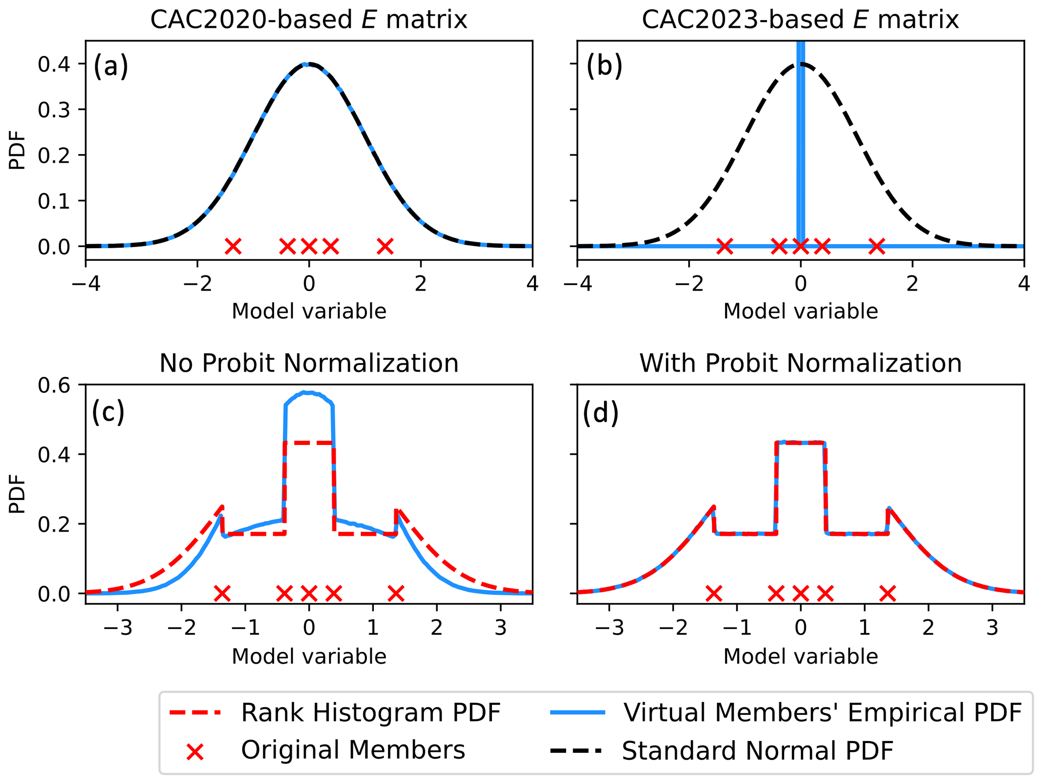
Figure 2 Plots demonstrating the impacts of various heuristic choices in the formulation of PESE-GC. Panels (a) and (b), respectively, demonstrate drawing virtual members using CAC2020's W (Eq. 7) and CAC2023's W (Eq. 10). The former produces Gaussian virtual members, while the latter produces non-Gaussian virtual members. Panels (c) and (d) demonstrate the importance of ensuring that the forecast ensemble in probit space has unit variance. If the probit-space forecast ensemble’s variance is not unity, the virtual members generated by PESE-GC will deviate from the fitted marginal PDFs (rank histogram in the case of panels c and d).

2.1.5 Properties of the CAC2020 algorithm

The CAC2020 algorithm is efficient and scales well with parallel computing. This is because steps 2 and 3 of the CAC2020 algorithm (Sect. 2.1.2 and 2.1.3) are embarrassingly parallel and have computational complexities that scale linearly with N_x. If E is generated offline (i.e., not part of the EnsDA procedure) and then read into the EnsDA program, the CAC2020 algorithm is reduced to only evaluating steps 2 and 3.

The CAC2020 algorithm also produces expanded ensembles with same ensemble means and ensemble covariances as the forecast ensembles. In other words, the rank of the expanded ensemble's covariance matrix is the same as that of the forecast ensemble. Future work can explore ways to incorporate localization into the expanded ensemble's covariance matrix.

Furthermore, the CAC2020 algorithm always generates Gaussian-distributed virtual members; even if the actual forecast distribution is highly non-Gaussian, the virtual members' distribution will still be Gaussian. The CAC2020 algorithm thus degrades the ensemble statistics in situations where the forecast distribution is non-Gaussian. This degradation limits the usefulness of the CAC2020 algorithm for situations with non-Gaussian forecast distributions.

Note that, except for the mean and covariance, the expanded ensemble's central moments (i.e., higher-order moments; e.g., skewness) likely differ from the forecast ensemble's. More specifically, the expanded ensemble's central moments will be closer to those of Gaussian distributions (e.g., zero skewness) than the forecast ensemble's central moments. This is because the virtual members are effectively drawn from a Gaussian distribution. If the forecast distribution is indeed a Gaussian distribution, then the expanded ensemble likely has better moments than the forecast ensemble.

2.2 The PESE-GC procedure

The CAC2020 algorithm is limited to generating Gaussian-distributed virtual members. PESE-GC overcomes this limitation by combining probit probability integral (PPI) transforms and their inverses with the CAC2020 algorithm. A PPI transform transforms any univariate distribution with a continuous CDF into a standard normal distribution, and the inverse PPI transform reverses the process. The quantity resulting from applying the PPI transform on a random variable is called “probit” and the coordinate space occupied by probits is called “probit space”. Such transforms are often used in Gaussian anamorphosis (Amezcua and Van Leeuwen, 2014; Grooms, 2022).

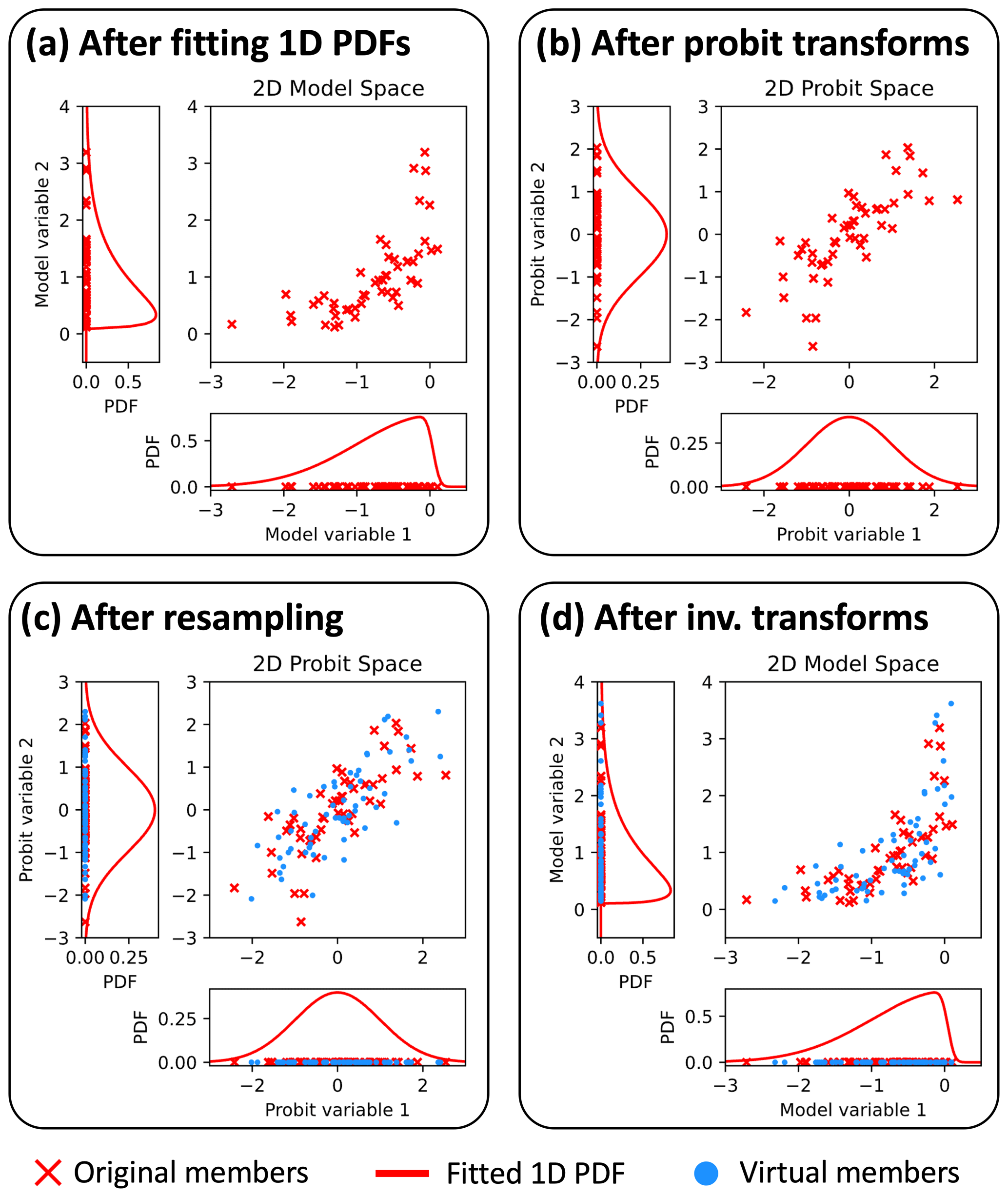
Figure 3 Illustrations of PESE-GC’s four-stage algorithm. Panels (a), (b), (c), and (d), respectively, show the aftermath of stages 1, 2, 3, and 4. The details of these stages are described in Sect. 2.2. Note that the CAC2020 algorithm is applied in stage 3 (i.e., between panels c and d).

To define the PPI transform, suppose F_i(x_i) represents the CDF of the ith model variable, x_i ($i=\mathrm{1},\mathrm{2},\mathrm{\dots },N_x$); Φ⁻¹(q) represents the inverse CDF of the standard normal (q represents any quantile); and ϕ_i represents the ith model probit. The double appearance of index i in F_i(x_i) is deliberate – the CDF varies with the chosen model variable. Note that Φ⁻¹(q) is sometimes called the probit function or the quantile function of the standard normal. The conversion from x_i to ϕ_i (i.e., the PPI transform) is

$$\begin{array}{}\text{(11)}& {\mathit{\varphi }}_i\equiv {\mathrm{\Phi }}^{-\mathrm{1}}\left(F_i\left(x_i\right)\right).\end{array}$$

The inverse PPI transform (i.e., converting ϕ_i to x_i) is

$$\begin{array}{}\text{(12)}& x_i\equiv F_i^{-\mathrm{1}}\left(\mathrm{\Phi }\left({\mathit{\varphi }}_i\right)\right).\end{array}$$

The PPI transform generalizes the CAC2020 algorithm to handle non-Gaussian forecast ensembles. The resulting PESE-GC procedure has four stages and is illustrated in Fig. 3. These four stages are as follows:

1. For each model state variable, fit a user-specified univariate distribution to that model variable in the forecast ensemble (i.e., marginal distribution fitting).

2. For each model state variable, apply the PPI transform (Eq. 11) using that variable's fitted distribution to convert the forecast ensemble of that model variable into forecast probits.

3. For each model state variable, adjust the mean and variance of that variable's forecast ensemble probits to zero and unity, respectively (explained in Sect. 2.3), and then apply the CAC2020 algorithm on that variable's forecast probits to generate virtual probits.

4. For each model state variable, apply the inverse PPI transform (Eq. (12) with stage 1's fitted distribution on that variable's virtual probits to generate that variable's virtual ensemble.

To be clear, the CAC2020 algorithm is implemented and used in stage 3.

Note that this four-stage procedure assumes that the multivariate forecast distribution is Gaussian in probit space. This assumption arises from the use of a Gaussian resampling algorithm (the CAC2020 algorithm) to generate virtual probits. This assumption is equivalent to assuming that the multivariate forecast distribution has a Gaussian copula. As such, this four-stage procedure is called Probit-space Ensemble Size Expansion for Gaussian Copulas.

PESE-GC's four-stage procedure is attractive for geophysical EnsDA for several reasons. Aside from the fact that it can generate non-Gaussian virtual members, PESE-GC can be implemented in an embarrassingly parallel fashion (every loop over the model state variables is embarrassingly parallel). Furthermore, PESE-GC is likely affordable for geophysical EnsDA because the CAC2020 algorithm (stage 3) is efficient (see Sect. 2.1).

Note that the quality of the virtual members depends on the distributions the user selects in step 1 of PESE-GC. This will be discussed later in Sect. 3.

2.3 On the mean and variance adjustments in PESE-GC's step 3

PESE-GC requires forecast ensemble probits with zero mean and unity variance. Otherwise, the resulting virtual members will disobey the marginal distributions fitted in PESE-GC's step 1. However, because the forecast ensemble size is finite, the forecast ensemble's probits may have non-zero mean and non-unity variance. To illustrate, suppose PESE-GC is applied to five univariate forecast ensemble members (red crosses in Fig. 2c) and a Gaussian-tailed rank histogram distribution (Anderson, 2010) is fitted to those five members in PESE-GC's step 1. Applying the PPI transform (PESE-GC's step 2) results in forecast probits with a mean of zero and a variance of approximately 0.561. Using the CAC2020 algorithm, 10⁷ virtual probits are then generated from these forecast probits, and the inverse PPI transform is applied to generate the virtual members (PESE-GC's step 4). The histogram-estimated PDF of the virtual members (blue curve in Fig. 2c) disagrees with the fitted (i.e., desired) Gaussian-tailed rank histogram PDF.

This problematic disagreement is resolved by adjusting the forecast probits' mean and variance to zero and unity (respectively) before generating the virtual members. Suppose the probit of the nth forecast member for model variable i is ϕ_i,n and the pre-adjusted prior ensemble probit's sample mean and sample variance are μ and σ², respectively. The adjustment process is simply

$$\begin{array}{}\text{(13)}& {\mathit{\varphi }}_{i,n}\leftarrow {\displaystyle \frac{{\mathit{\varphi }}_{i,n}-\mathit{\mu }}{\mathit{\sigma }}}\forall n=\mathrm{1},\mathrm{2},\mathrm{\dots },N_{\mathrm{E}}.\end{array}$$

The impact of this adjustment is illustrated in Fig. 2: the virtual members' histogram-estimated PDF (blue curve in Fig. 2d) now matches the Gaussian-tailed rank histogram PDF in PESE-GC's step 1.

3 Conceptual exploration of PESE-GC's EnsDA impacts

To understand the influence of PESE-GC on EnsDA, consider a joint model–observation space formulation of Bayes' rule:

$$\begin{array}{}\text{(14)}& p\left(\mathit{\psi }|{\mathit{y}}^{\mathrm{o}}\right)\propto p\left({\mathit{y}}^{\mathrm{o}}|\mathit{\psi }\right)p\left(\mathit{\psi }\right),\end{array}$$

where y^o is an N_y-dimensional vector of observation values, and

$$\begin{array}{}\text{(15)}& \mathit{\psi }\equiv \left[\begin{array}{c}\mathit{x}\\ \mathit{h}\left(\mathit{x}\right)\end{array}\right],\end{array}$$

where h(x) is the observation operator, p(y^o|ψ) is the observation likelihood function, and p(ψ) is the prior probability density function (PDF). The goal of EnsDA is to obtain a posterior ensemble that represents the posterior distribution p(ψ|y^o). If PESE-GC alters p(y^o|ψ) and/or p(ψ), then PESE-GC will influence EnsDA. As such, there are two potential mechanisms for PESE-GC to influence EnsDA: (1) alterations to the observation likelihood used by the EnsDA algorithm and (2) alterations to the prior distribution used by the EnsDA.

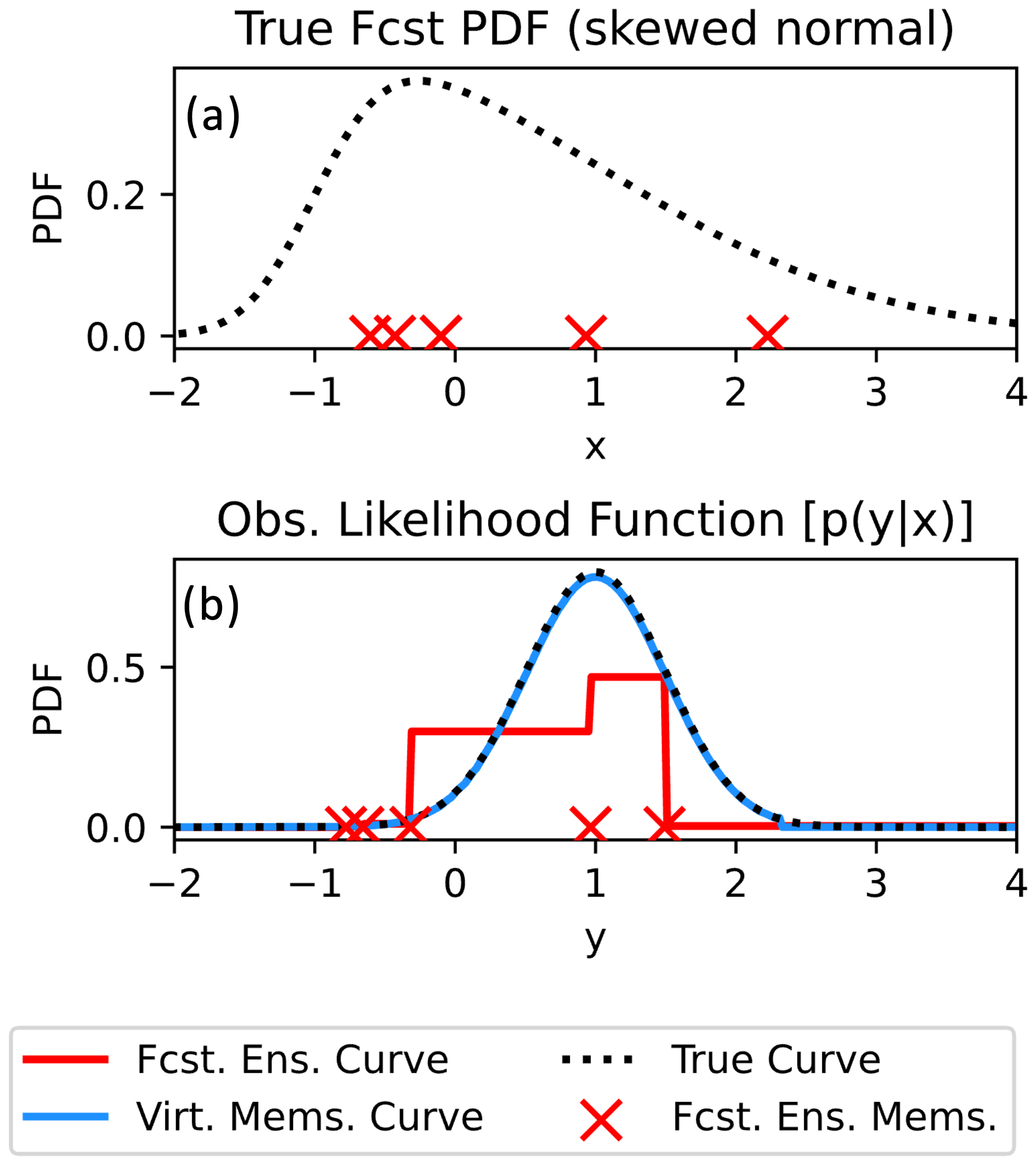
Figure 4 Plots of the true forecast PDF (a) and observation likelihood functions (b). The five forecast ensemble x values are indicated with red crosses in (a), and the five forecast ensemble y values are indicated with red crosses in (b). The red curve in (b) indicates the piecewise-approximated observation likelihood function used by a rank histogram filter that only uses the five forecast members. With PESE-GC, the rank histogram filter's piecewise-approximated observation likelihood function (blue curve) is improved.

This section explores the influence of PESE-GC on EnsDA through those two mechanisms. A bivariate example is used to illustrate those mechanisms. Suppose a scalar forecast model variable x has a skewed normal forecast distribution and five samples are drawn from this distribution (illustrated in Fig. 4a). A signed square root function (h(x))

$$\begin{array}{}\text{(16)}& h\left(x\right)\equiv \text{sign}\left(x\right)\sqrt{\left|x\right|},\end{array}$$

is used as the observation operator, and let y denote observation values. In this bivariate example, 10 000 virtual members will be generated by PESE-GC. Note that the true forecast distribution of x is the previously mentioned skewed normal distribution (illustrated in Fig. 4a), and the true forecast distribution of h(x) is estimated by applying h(x) to 1 million samples of x drawn from the true forecast distribution of x.

3.1 Mechanism 1: PESE-GC improves ensemble-based representation of the observation likelihood function

For certain EnsDA algorithms that employ ensemble-based representations of the observation likelihood function, PESE-GC can improve those representations (impact mechanism 1). Two EnsDA algorithms will be considered: (1) the rank histogram filter (RHF; Anderson, 2010) and (2) the serial stochastic ensemble Kalman filter (serial stochastic EnKF; Burgers et al., 1998). In the case of the RHF, an ensemble-based piecewise approximation of the observation likelihood function is used (illustrated in Fig. 4b). The accuracy of that piecewise approximation depends on the ensemble size. When small forecast ensembles are used, that piecewise approximation is crude (red curve in Fig. 4b). Since PESE-GC increases ensemble size, PESE-GC refines that piecewise representation (blue curve in Fig. 4b). In the absence of other factors, this refinement will improve the performance of the RHF.

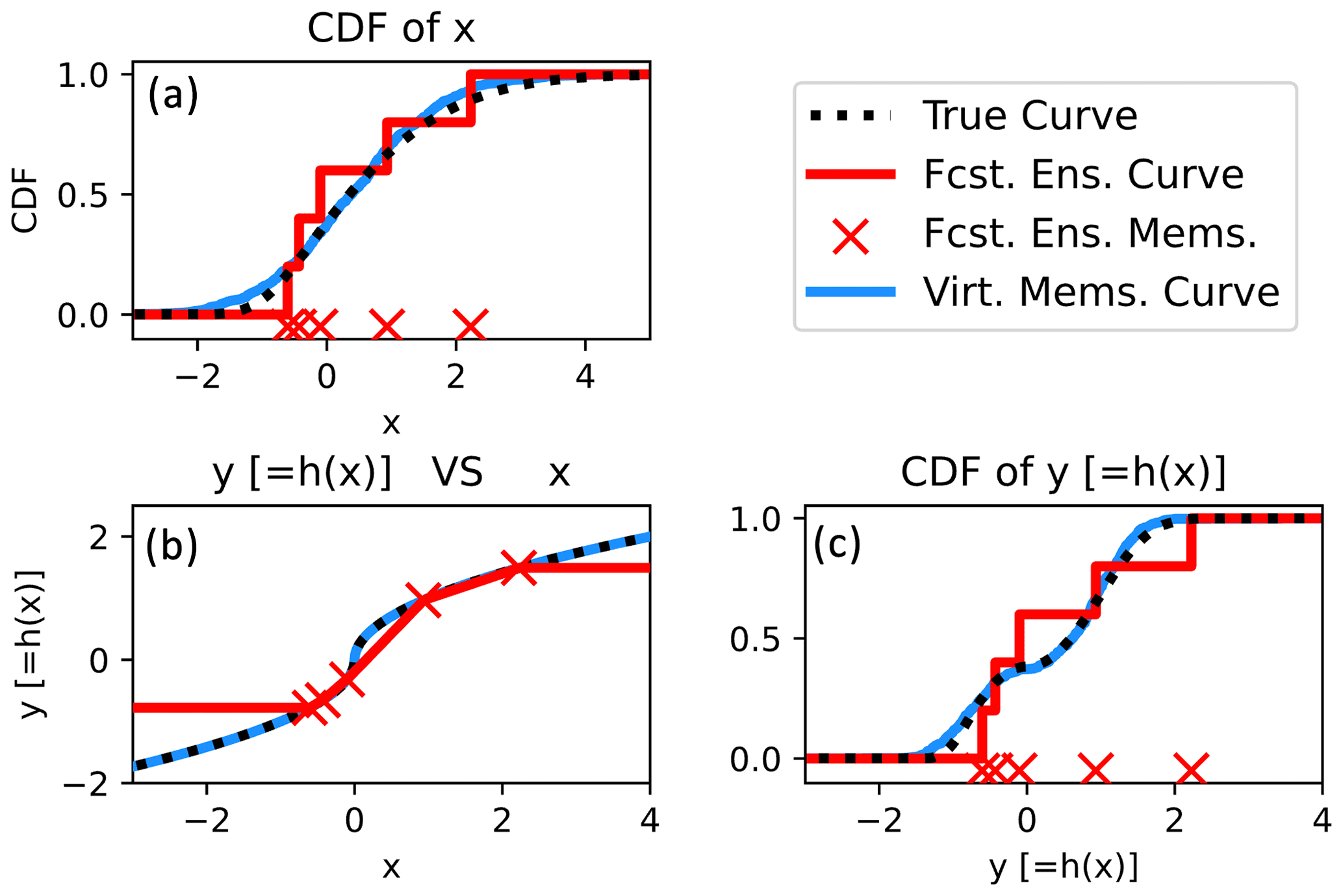
Figure 5 Bivariate example demonstrating the impacts of drawing virtual members from an informative fitted marginal (normal distribution). Panel (a) shows the empirical CDFs of x from the initial members and virtual members. The estimated relationships between x and y (obtained by passing the initial members and virtual members through h(x)) are displayed in panel (b). Finally, panel (c) shows the empirical CDFs of the initial members and virtual members for variable y. The true CDFs and x–y relationships are plotted in panels (b) and (c) with dotted black lines.

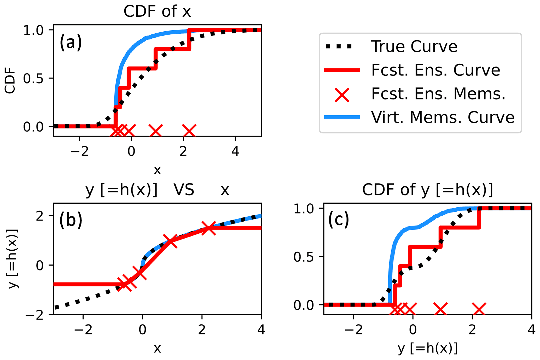
Figure 6 Bivariate example demonstrating the impacts of drawing virtual members from a misinformed fitted marginal (gamma distribution). The panels here are similar to Fig. 5.

Impact mechanism 1 also manifests for the serial stochastic EnKF. To see that, consider a situation with two observations and recall that the serial stochastic EnKF uses random draws from a univariate Gaussian distribution to represent the likelihood function (one draw per ensemble member). For small ensembles, only a few of those random draws are made. In other words, there are sampling errors in representing the likelihood function. The ensemble statistics resulting from assimilating the first observation are thus degraded by those sampling errors. This degradation then affects the assimilation of the second observation. The assimilation of more than two observations compounds such sampling issues. Since PESE-GC increases the ensemble size, more draws from the likelihood function are made, thus suppressing sampling errors. As such, in the absence of other factors, PESE-GC will improve the performance of the serial stochastic EnKF.

Note that many EnsDA algorithms are immune to impact mechanism 1. The deterministic variants of the EnKF (Bishop et al., 2001; Whitaker and Hamill, 2002; Anderson, 2003; Tippett et al., 2003; Sakov and Oke, 2008) and particle filters (Gordon et al., 1993; Snyder et al., 2008; Poterjoy, 2016; van Leeuwen et al., 2019) are immune to impact mechanism 1 because no ensemble-based representation of the likelihood function is used. Also, the stochastic EnKF that assimilates all observations simultaneously (all-at-once stochastic EnKF) is immune to this effect – the chain of events described in the previous paragraph will not occur for the all-at-once stochastic EnKF. Finally, EnsDA systems that run ensembles of variational data assimilation methods (e.g., the ECMWF) are also immune to impact mechanism 1. This immunity is due to the same reason as the all-at-once stochastic EnKF.

3.2 Mechanism 2: PESE-GC influences ensemble statistics

If the user specifies appropriate marginals in PESE-GC's stage 1, then PESE-GC will improve the ensemble statistics used by EnsDA algorithms (mechanism 2). This will be illustrated using the bivariate five-member example discussed near the start of Sect. 3. Suppose the user knows that the prior marginal distribution of x is close to Gaussian. Thus, a Gaussian distribution is fitted to the forecast x values in PESE-GC's stage 1 (Sect. 2.2; Fig. 5a). Applying PESE-GC generates 10 000 virtual members. Figure 5 indicates that the virtual members' CDFs and x–y relationship are closer to the true CDFs and relationship than those of the forecast members – the virtual members' curves have visibly shorter distances from the true curves than the forecast members' curves. In other words, the virtual members have better ensemble statistics than the forecast ensemble. This improvement in ensemble statistics is a combination of (1) the user selecting an appropriate marginal for x and (2) the nonlinear h(x) is evaluated more often (i.e., sampled better) with a large ensemble. As such, if the user specifies appropriate marginals in PESE-GC's stage 1, PESE-GC will likely improve the performance of EnsDA algorithms.

An important caveat is that if the user selects misinformed marginal distributions, then PESE-GC may degrade the ensemble statistics used by EnsDA algorithms. To illustrate, suppose the user fits a shifted gamma distribution (Cheng and Amin, 1983) to the five forecast x values. This distribution has three parameters: shape, scale, and location. Since only five forecast values are used to fit three parameters, the fitted parameters' sampling errors are severe. Applying PESE-GC with this badly estimated shifted gamma distribution results in virtual ensemble statistics that are worse than those of five forecast x values (Fig. 6). In such situations, the performance of EnsDA will likely be degraded by PESE-GC. As such, the selection of marginals to use with PESE-GC must be done with care.

In the absence of knowledge about the model variables' prior marginal distribution, users can use non-parametric marginal distributions with PESE-GC. Such distributions include the Gaussian-tailed rank histogram distribution (Anderson, 2010) and kernel distributions (Anderson and Anderson, 1999). Choosing such distributions may not improve the model-space ensemble statistics. However, because PESE-GC increases the number of observation operator evaluations, the observation-space ensemble statistics and the ensemble covariance/copula between observation and model quantities can be improved.

Note that when linear observations are assimilated, PESE-GC with Gaussian marginals will not change the performance of deterministic variants of the EnKF (Bishop et al., 2001; Whitaker and Hamill, 2002; Anderson, 2003; Tippett et al., 2003; Sakov and Oke, 2008). This is because the expanded ensemble will have the same joint-space mean and covariance as the forecast ensemble.

4 Tests with Lorenz 1996 model

4.1 Setup of experiments

This section explores the impacts of PESE-GC on the performance of EnsDA using perfect model Observing System Simulation Experiments (OSSEs) with the Lorenz 1996 model (L96 model; Lorenz, 2006). The Data Assimilation Research Testbed (DART; https://github.com/NCAR/DART, last access: 13 May 2023; National Center for Atmospheric Research, 2024; Anderson et al., 2009) is used in this exploration, and PESE-GC has been implemented into the version of DART archived at https://doi.org/10.5281/zenodo.10126956 (Chan, 2023).

The L96 model uses 40 variables (i.e., 40 grid points in a ring), a forcing parameter value of 8 (i.e., F=8), and a time step of 0.05 L96 time units. The L96 time unit is henceforth referred to as τ. All results in this paper are displayed and discussed in terms of τ. Forward time integration of the model is done via the Runge–Kutta fourth-order integration scheme. Every OSSE runs for 5500 cycles. Initial nature run states and the initial ensemble members are drawn from L96's climatology.

In all experiments, there are 40 observations. Their observation locations are fixed throughout this study. Supposing that the model grid points have locations 0.025m, $m=\mathrm{1},\mathrm{2},\mathrm{\dots },\mathrm{40}$, each site location is a random draw from a uniform distribution between 0 and 1.

PESE-GC's impacts are examined using EnsDA experiments that are conducted with four N_Es, five cycling intervals, three post-PESE-GC ensemble sizes, three observation types, four EnsDA algorithms, and with and without PESE-GC, a total of $\mathrm{4}\times \mathrm{5}\times \mathrm{3}\times \mathrm{3}\times \mathrm{4}\times \mathrm{2}=\mathrm{1440}$ configurations. The four N_Es are 10, 20, 40, and 80, and the five cycling intervals are 0.05τ, 0.10τ, 0.15τ, 0.30τ, and 0.60τ.

The PESE-GC-expanded ensemble sizes are specified in terms of factors: 5, 10, and 20 times the forecast ensemble size. For example, if N_E=10, a PESE-GC factor of 10 means that the expanded ensemble has 100 members (i.e., N_V=90 virtual members are created).

Supposing the kth observation site has location ℓ_k, the observation operators for the three observation types are

$$\begin{array}{}\text{(17)}& {\displaystyle }{h}_{\mathrm{IDEN}}\left(\mathit{x};{\mathrm{\ell }}_k\right)\equiv x_{{\mathrm{\ell }}_k},\text{(18)}& {\displaystyle }{h}_{\mathrm{SQRT}}\left(\mathit{x};{\mathrm{\ell }}_k\right)\equiv \mathrm{sgn}\left(x_{{\mathrm{\ell }}_k}\right)\sqrt{\left|x_{{\mathrm{\ell }}_k}\right|},\text{(19)}& {\displaystyle }{h}_{\mathrm{SQUARE}}\left(\mathit{x};{\mathrm{\ell }}_k\right)\equiv \mathrm{sgn}\left(x_{{\mathrm{\ell }}_k}\right){\left(x_{{\mathrm{\ell }}_k}\right)}^{\mathrm{2}},\end{array}$$

where x is the L96 model's 40-element state vector, $x_{{\mathrm{\ell }}_k}$ is the model variable linearly interpolated to location ℓ_k, and $\mathrm{sgn}\left(x_{{\mathrm{\ell }}_k}\right)$ returns the sign of $x_{{\mathrm{\ell }}_k}$. Observations created using h_IDEN(x;ℓ_k), h_SQRT(x;ℓ_k), and h_SQUARE(x;ℓ_k) are henceforth respectively referred to as IDEN observations, SQRT observations, and SQUARE observations. Every observation is created by applying its corresponding observation operator to a nature run state and then perturbing the output with a random draw from 𝒩(0,σ²). Following Anderson (2020), the chosen σ² for the IDEN, SQRT, and SQUARE observations are 1.0, 0.25, and 16, respectively. Note that IDEN's σ² is between 7.4 % and 15 % of the climatological IDEN error variance, SQRT's σ² is between 10 % and 17 % of the climatological SQRT error variance, and SQUARE's σ² is between 2 % and 6 % of the climatological SQUARE error variance.

The four EnsDA algorithms tested with PESE-GC are

1. the ensemble adjustment Kalman filter (EAKF; Anderson, 2003)

2. the serial stochastic EnKF with sorted observation increments (EnKF; Burgers et al., 1998)

3. the rank histogram filter with linear regression (RHF; Anderson, 2010)

4. the rank histogram filter with probit regression (PR; Anderson, 2023).

To be clear, the RHF algorithm first employs the rank histogram filter to generate observation increments and then uses linear regression to convert observation increments into model increments. The PR algorithm is similar to the RHF algorithm, except that probit regression is used to convert observation increments into model increments.

For each EnsDA algorithm, only one set of marginals is used with PESE-GC. When PESE-GC is used with the EAKF, EnKF, or RHF algorithm, Gaussian marginals are selected for all 40 model variables. PESE-GC with Gaussian marginals is identical to the CAC2020 algorithm. In other words, for the EAKF, EnKF, and RHF experiments, the virtual ensemble members follow multivariate Gaussian distributions. For the PR algorithm, the Gaussian-tailed rank histogram is selected as the marginal for every one of the 40 model variables. This means the PR experiments' virtual ensemble members follow multivariate non-Gaussian distributions. Future work can investigate the impacts of using PESE-GC with Gaussian-tailed rank histograms (or kernel density estimates) with the EAKF, EnKF, and RHF.

Each of the 1440 configurations is trialed 36 times. These trials are enumerated (Trial 1, Trial 2, and so forth). All experiments with the same trial number and N_E share the same nature run and initial forecast ensemble states. For example, the following two EnsDA experiments have the same initial nature run and initial forecast ensemble: (1) Trial 10 using IDEN observations, 20 forecast ensemble members, 0.15τ cycling period, EAKF, and PESE-GC with an expansion factor of 20 and (2) Trial 10 using SQRT observations, 20 forecast ensemble members, 0.60τ cycling period, RHF, and PESE-GC with an expansion factor of 5. Note that experiments with different trial numbers have different nature runs and initial forecast ensemble states.

The Gaspari–Cohn fifth-order rational function (Gaspari and Cohn, 1999) is used to localize EnsDA increments. For each combination of trial and configuration, 17 localization half-radii are tested: $\mathrm{0.075}\times {\mathrm{1.3}}^{\mathrm{0}},\mathrm{0.075}\times {\mathrm{1.3}}^{\mathrm{1}},\mathrm{0.075}\times {\mathrm{1.3}}^{\mathrm{2}},\mathrm{0.075}\times {\mathrm{1.3}}^{\mathrm{3}},\mathrm{\dots },\mathrm{0.075}\times {\mathrm{1.3}}^{\mathrm{14}},\mathrm{0.075}\times {\mathrm{1.3}}^{\mathrm{15}}$, and infinity. To select the optimal localization half-radius for a given combination of trial and configuration, the root-mean-square error (RMSE) of the forecast ensemble mean is used. The RMSE for a particular cycle is

$$\begin{array}{}\text{(20)}& \text{RMSE}\equiv \sqrt{{\displaystyle \frac{\mathrm{1}}{\mathrm{40}}}\sum _{i=\mathrm{1}}^{\mathrm{40}}{\left(\stackrel{\mathrm{‾}}{x_i^{\mathrm{f}}}-x_i^t\right)}^{\mathrm{2}}},\end{array}$$

where $\stackrel{\mathrm{‾}}{x_i^{\mathrm{f}}}$ and $x_i^t$ are, respectively, the forecast ensemble mean state and nature run state at model grid point i. The RMSEs of the first 500 out of 5500 EnsDA cycles are discarded. The localization half-radius that results in the smallest cycle-averaged RMSE (i.e., averaged from cycles 501 to 5500) is selected as the optimal localization half-radius. Note that for the same configuration, the optimal localization half-radius can vary with the trial number.

The inflation scheme used here is identical to the one used by Anderson (2023). The adaptive prior inflation algorithm of Anderson (2009) is used with an inflation lower bound of 1 (no deflation), an upper bound of 2, a fixed inflation standard deviation of 0.6, and an inflation damping of 0.9. While manually tuning a homogeneous inflation factor or a relaxation-to-posterior-spread (RTPS; Whitaker and Hamill, 2012) relaxation factor may give smaller RMSEs, an adaptive inflation approach is chosen to reduce the computational cost of this study. This study already runs 881 280 ($\mathrm{1440}\times \mathrm{36}\times \mathrm{17}$) combinations of configurations (1440), trials (36), and localization half-radii (17), and each combination is run for 5500 cycles.

4.2 Metric to assess PESE-GC's impact on EnsDA

The impacts of PESE-GC on EnsDA are assessed using the relative difference between cycle-averaged RMSEs (Eq. 20) with PESE-GC and cycle-averaged RMSEs without PESE-GC. The cycle averaging is done from cycles 501 to 5500. To define this RMSE relative difference, suppose an arbitrary configuration of N_E, cycling interval, PESE-GC factor, observation type, and EnsDA algorithm is denoted by ξ. Let $\stackrel{\mathrm{‾}}{\text{RMSE}\left(\mathit{\xi },r,\text{True}\right)}$ denote the cycle-averaged RMSE of the rth trial of configuration ξ with PESE-GC used. Furthermore, let $\stackrel{\mathrm{‾}}{\text{RMSE}\left(\mathit{\xi },r,\text{False}\right)}$ denote the cycle-averaged RMSE of the rth trial of configuration ξ without using PESE-GC. The relative difference between $\stackrel{\mathrm{‾}}{\text{RMSE}\left(\mathit{\xi },r,\text{True}\right)}$ and $\stackrel{\mathrm{‾}}{\text{RMSE}\left(\mathit{\xi },r,\text{False}\right)}$ is defined as

$$\begin{array}{}\text{(21)}& \mathrm{\Delta }\text{RMSE}\left(\mathit{\xi },r\right)\equiv {\displaystyle \frac{\text{RMSE}\left(\mathit{\xi },r,\text{True}\right)-\text{RMSE}\left(\mathit{\xi },r,\text{False}\right)}{〈\stackrel{\mathrm{‾}}{\text{RMSE}\left(\mathit{\xi },\text{False}\right)}〉}}.\end{array}$$

Here, the denominator is the trial-averaged (indicated by angled brackets) cycle-averaged RMSE of the EnsDA run with the same ξ as in the numerator but with PESE-GC unused. For readability, (ξ,r) is omitted from the rest of this paper. Most importantly, a negative ΔRMSE indicates that PESE-GC improves the performance of EnsDA, and a positive value of ΔRMSE indicates that PESE-GC degrades the performance of EnsDA.

Only statistically significant trial-averaged ΔRMSE (henceforth 〈ΔRMSE〉) is discussed in this paper. A 〈ΔRMSE〉 is considered statistically significant if its two-tailed z-test p value is smaller than 1 %. These statistically significant 〈ΔRMSE〉 values are plotted in Figs. 7, 8, and 9.

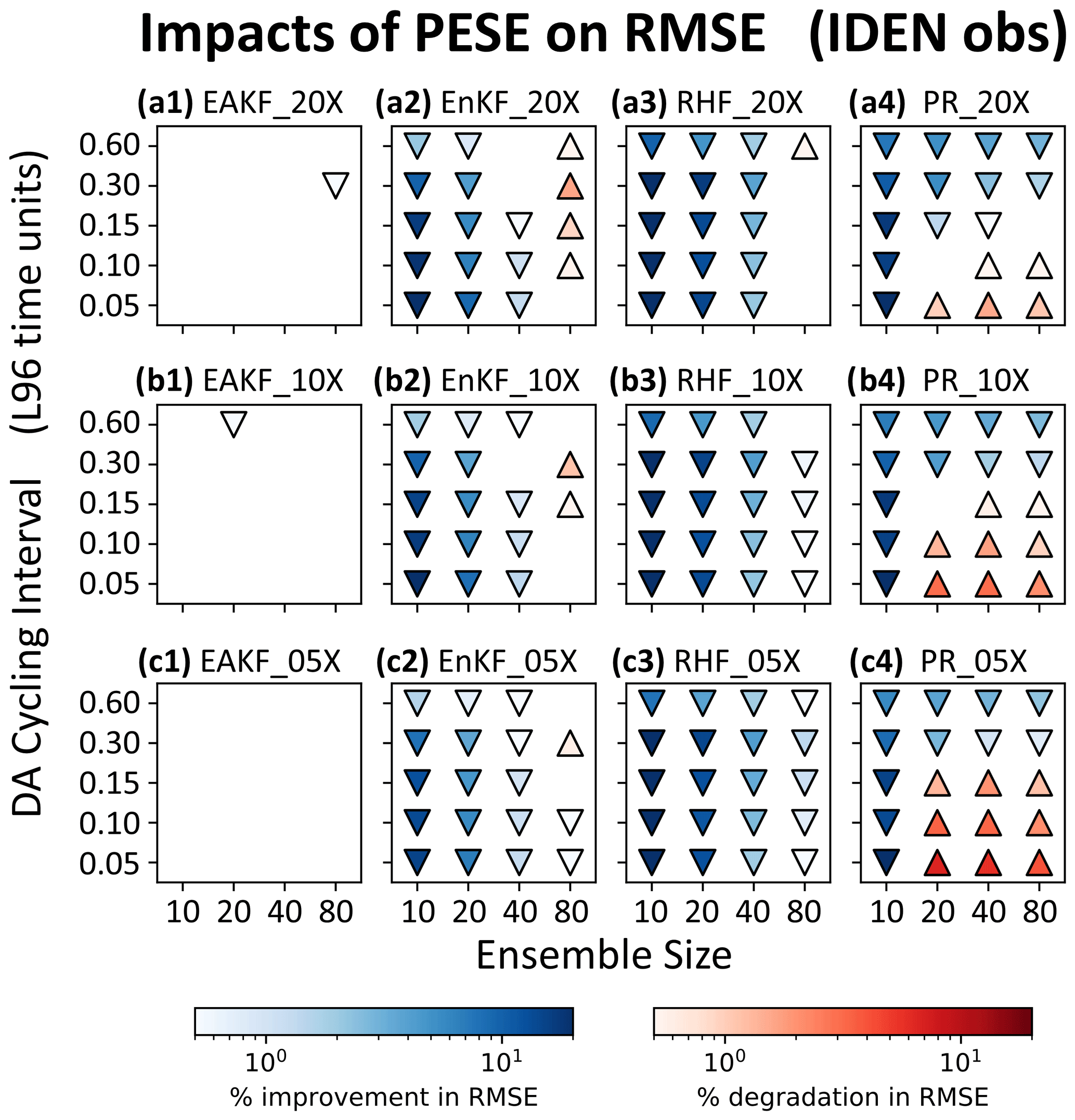
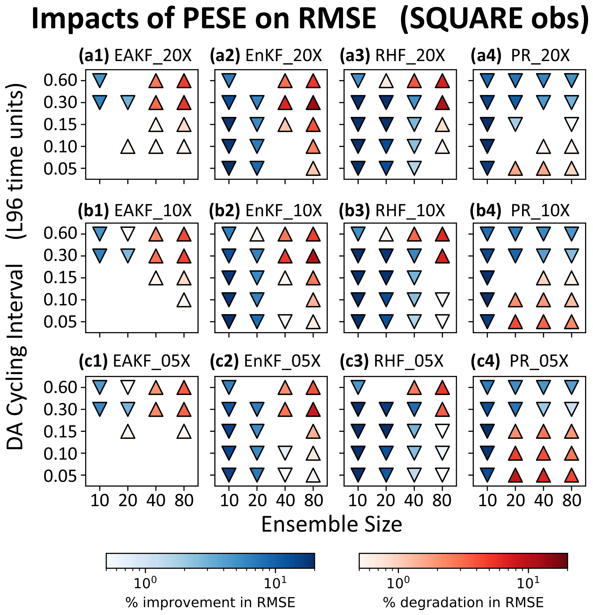
Figure 7 Statistically significant 〈ΔRMSE〉 values (two-tailed p<0.01) for pairs of PESE-GC-using and PESE-GC-omitting experiments that assimilate IDEN observations. The PESE-GC-using EnsDA experiments in panels (a1), (a2), (a3), and (a4) expanded their forecast ensembles 20-fold, the PESE-GC-using EnsDA experiments in panels (b1), (b2), (b3), and (b4) expanded their forecast ensembles 10-fold, and the PESE-GC-using EnsDA experiments in panels (c1), (c2), (c3), and (c4) expanded their forecast ensembles fivefold. Panels (a1), (b1), and (c1) show 〈ΔRMSE〉 for EnsDA experiments using the EAKF, panels (a2), (b2), and (c2) show 〈ΔRMSE〉 for EnsDA experiments using the EnKF, panels (a3), (b3), and (c3) show 〈ΔRMSE〉 for EnsDA experiments using the RHF, and panels (a4), (b4), and (c4) show 〈ΔRMSE〉 for EnsDA experiments using the PR. The acronyms are defined in Sect. 4.1. Downward triangles indicate 〈ΔRMSE〉<0 and upward triangles indicate 〈ΔRMSE〉>0.

Figure 8 Similar to Fig. 7, except that SQRT observations are assimilated.

Figure 9 Similar to Fig. 7, except that SQUARE observations are assimilated.

Before proceeding, note that PESE-GC with Gaussian marginals only negligibly changes the performance of the EAKF with IDEN observations (Fig. 7a1, b1, and c1). This negligibility is predicted in Sect. 3.2. Any impact of PESE-GC on the performance of these experiments is likely due to rounding errors associated with the use of finite precision arithmetic.

4.3 Impacts of using 20-fold PESE-GC on EnsDA

This study first examines the 〈ΔRMSE〉 for a PESE-GC factor of 20 (panels a1, a2, a3, and a4 in Figs. 7, 8, and 9). The focus is on identifying common patterns in 〈ΔRMSE〉 and explaining them through the lens of the two mechanisms laid out in Sect. 3. The variation in 〈ΔRMSE〉 with different PESE-GC factors (remaining panels in Figs. 7, 8, and 9) is discussed in Sect. 4.4.

The first common 〈ΔRMSE〉 pattern in the 20-fold PESE-GC situations is that PESE-GC generally improves EnsDA performance (i.e., 〈ΔRMSE〉<0) when N_E is 10 or 20 (panels a1, a2, a3, and a4 in Figs. 7, 8, and 9). This is because either one or both mechanisms described in Sect. 3 are acting to improve RMSEs. First, for the PR, RHF, and EnKF experiments, the performance improvements are partly (if not entirely) because PESE-GC improves the ensemble-based representation of the likelihood function (i.e., mechanism 1; Sect. 3.1). For the PR experiments with IDEN observations, mechanism 1 is likely the sole reason for the improved performance. Second, the PESE-GC-induced RMSE reductions in all 10/20 forecast member experiments with either SQRT or SQUARE observations are partly due to improved sampling of the observation operator (i.e., mechanism 2 described in Sect. 3.2).

The RMSE reductions seen in the 10/20-member EAKF, EnKF, and RHF experiments are also partly due to improved ensemble statistics (i.e., mechanism 2; Sect. 3.2). This is because the L96 model's forecast statistics tend to be close to Gaussian (e.g., Chan et al., 2020). Applying PESE-GC with Gaussian marginals thus improves the model variables' prior ensemble statistics, therefore improving the performance of the EAKF, EnKF, and RHF experiments.

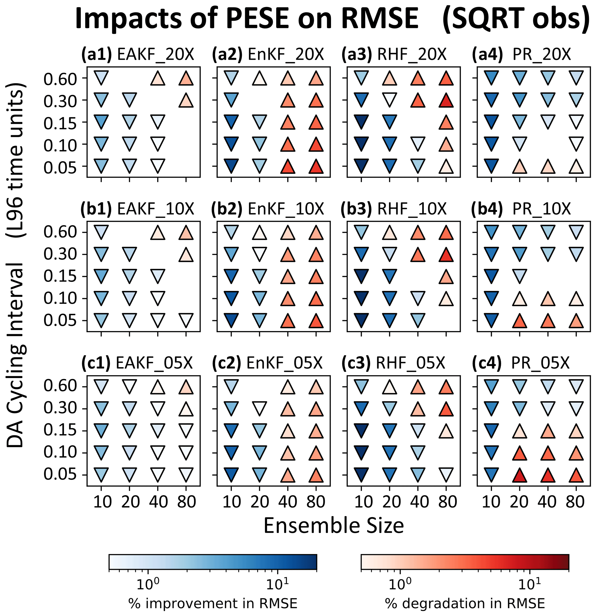
The second common pattern in the 20-fold PESE-GC experiments is that with increasing N_E, PESE-GC's RMSE impacts can go from improving (〈ΔRMSE〉<0) to degrading (〈ΔRMSE〉>0). This pattern is likely related to both mechanisms in Sect. 3. First, for the EnKF, RHF, and PR, the ensemble-based representation of the observation likelihood function improves with increasing N_E. This improvement implies there is less room for PESE-GC to improve that representation. As such, mechanism 1 weakens with increasing N_E, thus reducing PESE-GC-induced EnsDA performance gains for the EnKF, RHF, and PR EnsDA algorithms.

For the EAKF, EnKF, and RHF experiments, impact mechanism 2 also contributes to the worsening of PESE-GC's RMSE impacts with increasing N_E. In the act of choosing Gaussian marginal distributions for PESE-GC, the user implicitly assumes that the true forecast PDF is Gaussian. With increasing N_E, imperfections in this Gaussian assumption become increasingly evident. The impacts of PESE-GC on the observation space prior statistics can thus go from improving to degrading with increasing N_E. This change likely contributes to the worsening of PESE-GC's RMSE impacts with increasing N_E.

A third common pattern is that with longer cycles, the PESE-GC's RMSE impacts on the EAKF, EnKF, and RHF degrade (i.e., 〈ΔRMSE〉 goes from either negative to zero, zero to positive, or negative to positive). This pattern is likely due to increasing non-Gaussianity in the forecast ensemble's statistics with longer cycles. The choice to use Gaussian marginals in these experiments' PESE-GC thus becomes increasingly inappropriate, meaning that impact mechanism 2 increasingly degrades the performance of EnsDA.

The fourth common pattern is that in the PR experiments, for N_E≥20, the 20-fold PESE-GC's impact improves with longer cycling interval (Figs. 7a4, 8a4, and 9a4). A plausible explanation relates to PR's usage of a piecewise approximation to the observation likelihood function (henceforth the piecewise approximation). This approximation is more accurate when more ensemble members sample the regions of the observation likelihood function where that function varies strongly. However, with increasing forecast ensemble variance, those regions tend to be sampled less by forecast ensemble members, thus degrading the piecewise approximation. Since longer cycling intervals increase forecast ensemble variance, longer cycling intervals thus increase the room for PESE-GC to improve the piecewise approximation. Future work can test this explanation.

Note that the chain of events discussed in the previous paragraph likely occurs for the RHF experiments as well. Since the RHF experiments do not exhibit the fourth common pattern, it is likely that the inappropriateness of the Gaussian marginals used with PESE-GC overwhelms improvements introduced by refining the piecewise approximation.

4.4 Variations in PESE-GC's impacts with different amounts of ensemble expansion

This study now examines common patterns in how PESE-GC's impacts vary with PESE-GC expansion factors. The first common pattern is that PESE-GC's impacts on the PR experiments tend to weaken with smaller PESE-GC factors (panels a4, b4, and c4 in Figs. 7, 8, and 9). This pattern is likely caused by increasing sampling errors in the virtual members' statistics with fewer virtual members (i.e., smaller PESE-GC factors).

The second common pattern is that, for N_E≥40, smaller PESE-GC factors tend to result in milder RMSE degradations introduced by PESE-GC in the EAKF, EnKF, and RHF experiments. Since these RMSE degradations are likely due to the misinformed selection of Gaussian marginals with PESE-GC (see Sect. 4.3), reducing the number of virtual members reduces the amount of misinformation introduced by PESE-GC into the forecast statistics. These less misinformed forecast statistics explain the second common pattern.

An interesting third common pattern is also visible in the EAKF, EnKF, and RHF experiments: there are instances where reducing PESE-GC factors (1) turns insignificant RMSE impacts into RMSE improvements (e.g., the lower-left corner of Fig. 8a1 and c1) or (2) turns RMSE degradations into RMSE improvements (e.g., upper-right corner of Fig. 7a3 and c3). To explain this third pattern, notice that these instances are associated with short cycling intervals (0.05–0.10τ), and shorter cycling intervals are associated with increasingly Gaussian forecast PDFs. Based on these associations, a plausible explanation is that the true forecast statistics only mildly deviate from Gaussian, but the forecast ensemble statistics are often far from Gaussian. Introducing some Gaussian virtual members thus improves the ensemble statistics. However, if too many Gaussian virtual members are introduced, the expanded ensemble statistics become too close to Gaussian. This “Goldilocks” explanation can be tested in future work.

Most importantly, even with a mere fivefold PESE-GC, PESE-GC improves the performance of EnsDA in three types of situations. First, all EnsDA experiments involving small forecast ensemble sizes (10 members) are improved by PESE-GC. Second, situations where using Gaussian marginals with PESE-GC improves ensemble statistics are also improved by PESE-GC. This second type of situation occurs for the EAKF, EnKF, and RHF experiments that have either (1) 20–40 ensemble members and/or (2) cycling intervals that are 0.30τ or less. Third, PESE-GC improves the PR experiments for cycling intervals that are 0.30τ or 0.60τ. This improvement is plausibly because with longer cycling intervals, PESE-GC better improves the piecewise observation likelihood approximation used by the PR EnsDA algorithm (explained in Sect. 4.3). These PESE-GC-introduced improvements are particularly encouraging because a geophysical EnsDA system is more likely able to afford using 5-fold PESE-GC over 20-fold PESE-GC.

5 Discussion

5.1 PESE-GC assumes Gaussian copulas

The results presented in the previous section are encouraging. However, a caveat about PESE-GC needs discussion: PESE-GC assumes that the forecast distribution is a multivariate Gaussian distribution in probit space (i.e., Gaussian copula). If that assumption is violated (henceforth Gaussian copula assumption), the virtual members will possess statistical artifacts.

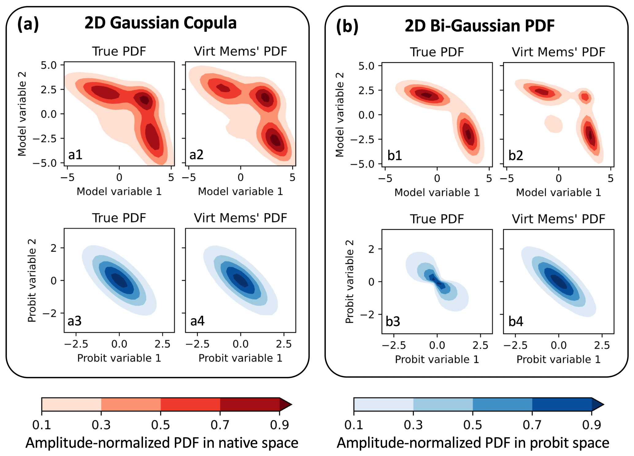
Figure 10 Two bivariate demonstrations of PESE-GC. In each demonstration, 100 initial members are drawn from a true bivariate PDF (a1, b1), bi-Gaussian PDFs are fitted to each variable, and PESE-GC creates 1 million virtual members. Panels (a1) and (b1) show the PDFs that the initial members are drawn from (i.e., the true bivariate PDFs), panels (a2) and (b2) show bivariate empirical PDFs estimated by the virtual members, panels (a3) and (b3) show the true bivariate PDF in probit space, and panels (a4) and (b4) show the virtual members’ bivariate empirical PDFs in probit space. The two true bivariate are a trimodal PDF with an underlying Gaussian copula (a1) and a bi-Gaussian PDF (d1). Note that the bi-Gaussian PDF’s copula is not a Gaussian copula (b3). The two true PDFs are described in Sect. 5.1.

Figure 10a illustrates PESE-GC's ability to generate non-Gaussian virtual members for a situation where the Gaussian copula assumption holds. The true forecast multivariate PDF (Fig. 10a1) is created by applying two inverse PPI transforms on a bivariate Gaussian PDF. The two-dimension mean vector μ and the 2×2 covariance matrix Σ of the bivariate Gaussian PDF are

$$\begin{array}{}\text{(22)}& {\displaystyle }\mathit{\mu }\equiv {\left[\begin{array}{cc}\mathrm{0}& \mathrm{0}\end{array}\right]}^{\top },\mathbf{\Sigma }\equiv \left[\begin{array}{cc}\mathrm{1}& \mathrm{0.7}\\ \mathrm{0.7}& \mathrm{1}\end{array}\right].\end{array}$$

The first inverse PPI transform is applied on the first variable (x₁) and the PDF it uses (p(x₁)) is

$$\begin{array}{}\text{(23)}& p\left(x_{\mathrm{1}}\right)\equiv {\displaystyle \frac{\mathrm{1}}{\mathrm{2}}}G\left(x_{\mathrm{1}};-\mathrm{1},\mathrm{2}\right)+{\displaystyle \frac{\mathrm{1}}{\mathrm{2}}}G\left(x_{\mathrm{1}};\mathrm{3},\mathrm{1}\right),\end{array}$$

where $G\left(x_{\mathrm{1}};-\mathrm{1},\mathrm{2}\right)$ represents the Gaussian PDF with a scalar mean of −1 and standard deviation of 2 and likewise for $G\left(x_{\mathrm{1}};\mathrm{3},\mathrm{1}\right)$. The second inverse PPI transform is applied on the second variable (x₂) and the PDF it uses (p(x₂)) is

$$\begin{array}{}\text{(24)}& {\displaystyle }p\left(x_{\mathrm{2}}\right)\equiv {\displaystyle \frac{\mathrm{1}}{\mathrm{2}}}G\left(x_{\mathrm{2}};\mathrm{2},\mathrm{1}\right)+{\displaystyle \frac{\mathrm{1}}{\mathrm{2}}}G\left(x_{\mathrm{2}};-\mathrm{2},\mathrm{2}\right),\end{array}$$

where $G\left(x_{\mathrm{2}};\mathrm{2},\mathrm{1}\right)$ and $G\left(x_{\mathrm{2}};-\mathrm{2},\mathrm{2}\right)$ are defined similarly to $G\left(x_{\mathrm{1}};-\mathrm{1},\mathrm{2}\right)$.

Since the forecast PDF in Fig. 10a1 has, by construction, a Gaussian copula (Fig. 10a3), PESE-GC can produce virtual members that approximately follow the forecast PDF. To demonstrate, 100 forecast members were drawn from the forecast PDF, and 1 million virtual members were constructed using PESE-GC. The two marginal PDFs that are used in steps 1, 2, and 4 of PESE-GC are univariate bi-Gaussian PDFs (fitted via a maximum likelihood estimation in step 1). The histogram-estimated PDFs of the virtual members (Fig. 10a2) and virtual probits (Fig. 10a4) are similar to the true forecast PDF (Fig. 10a1) and the true forecast's probit-space PDF (Fig. 10a3).

An example where the Gaussian copula assumption is violated is shown in Fig. 10b. Here, the forecast PDF (Fig. 10b1) is the following bivariate bi-Gaussian PDF

$$\begin{array}{}\text{(25)}& p\left(\mathit{x}\right)={\displaystyle \frac{\mathrm{1}}{\mathrm{2}}}G\left(\mathit{x};{\mathit{\mu }}_{\mathrm{1}},{\mathbf{\Sigma }}_{\mathrm{1}}\right)+{\displaystyle \frac{\mathrm{1}}{\mathrm{2}}}G\left(\mathit{x};{\mathit{\mu }}_{\mathrm{2}},{\mathbf{\Sigma }}_{\mathrm{2}}\right),\end{array}$$

where

$$\begin{array}{}\text{(26)}& {\displaystyle }\mathit{x}\equiv \left[\begin{array}{c}{x}_{\mathrm{1}}\\ x_{\mathrm{2}}\end{array}\right],{\mathit{\mu }}_{\mathrm{1}}\equiv \left[\begin{array}{c}-\mathrm{1}\\ \mathrm{2}\end{array}\right],{\mathit{\mu }}_{\mathrm{2}}\equiv \left[\begin{array}{c}\mathrm{3}\\ -\mathrm{2}\end{array}\right],\text{(27)}& {\displaystyle }{\mathbf{\Sigma }}_{\mathrm{1}}\equiv \left[\begin{array}{cc}\mathrm{2}& -\mathrm{0.5}\\ -\mathrm{0.5}& \mathrm{0.5}\end{array}\right],{\mathbf{\Sigma }}_{\mathrm{2}}\equiv \left[\begin{array}{cc}\mathrm{0.5}& -\mathrm{0.5}\\ -\mathrm{0.5}& \mathrm{2}\end{array}\right].\end{array}$$

Applying PPI transforms on this bivariate bi-Gaussian forecast PDF reveals that the bi-Gaussian PDF violates the Gaussian copula assumption (Fig. 10b3). When PESE-GC is applied to generate 1 million virtual members from 100 forecast members, the virtual members' probit space bivariate PDF (Fig. 10b4) differs from the forecast PDF in probit space (Fig. 10b3). As such, the virtual members' bivariate PDF (Fig. 10b2) deviates from the true bivariate bi-Gaussian forecast PDF (Fig. 10b1; the virtual members have two small spurious modes).

Note that though the virtual members' PDF deviates from the forecast PDF, a strong similarity exists between the two PDFs. The two dominant modes of the virtual members' PDF are very similar to the bi-Gaussian forecast PDF. More generally, milder violations of the Gaussian copula assumption will likely lead to milder spurious statistical features in the virtual members.

More importantly, PESE-GC's Gaussian copula assumption may not be problematic for geophysical EnsDA. Due to the high dimensionality of geophysical models and small forecast ensemble sizes, it is difficult to identify the family of the multivariate forecast distributions in probit space. In other words, the forecast ensemble's statistics in probit space are likely indistinguishable from a multivariate Gaussian. This indistinguishability permits assuming Gaussian copulas. Future work can investigate this possibility.

5.2 Impacts of PESE-GC on the computational cost of EnsDA

It is also important to discuss the impacts of PESE-GC on the EnsDA process (i.e., the forecast step and analysis step). Since the virtual members are deleted before running forecast models (Fig. 1), PESE-GC does not change the forecast step's computational cost. However, PESE-GC will increase the computational cost of the analysis step because (1) the number of observation operator calls scales linearly with the ensemble size and (2) the EnsDA filter algorithm's (e.g., the EAKF algorithm's) computational complexity scales with the ensemble size. Supposing the computational cost of the EnsDA filter algorithm scales linearly with ensemble size, then the computational cost of the EnsDA analysis step scales linearly with the number of ensemble members created by PESE-GC.

However, the increase in the computational cost associated with PESE-GC is likely far more affordable than running a larger forecast ensemble. This is because the computational cost of the forecast step often accounts for >80 % of the overall computational cost of the EnsDA process and the analysis step accounts for the remaining <20 %. Consider the situation where PESE-GC quintuples the ensemble size. The overall computational cost of the EnsDA process will only increase by <80 %. In contrast, if the forecast ensemble size is quintupled, then the overall computational cost of the EnsDA process increases by 400 %. As such, PESE-GC is an alluring alternative to increasing the forecast ensemble size.

6 Summary and future work

In this study, an efficient and embarrassingly parallel algorithm to increase ensemble sizes, PESE-GC, is formulated. PESE-GC generalizes the efficient and embarrassingly parallel Gaussian resampling algorithm of Chan et al. (2020) to handle non-Gaussian forecast distributions. This handling of non-Gaussian forecast distributions means PESE-GC is highly flexible. Furthermore, PESE-GC provides an avenue for users to use their knowledge of the forecast statistics to improve EnsDA – users can choose to draw virtual members using marginal distribution families (e.g., Gaussian and gamma distribution families) that they think are good approximations of the true forecast marginal distributions. If that knowledge is unavailable, users can choose to use non-parametric marginal distributions (e.g., Gaussian-tailed rank histogram distributions).

Three mechanisms are then identified for PESE-GC to influence the performance of EnsDA. First, for EnsDA methods like the serial stochastic EnKF and the rank histogram filter, PESE-GC improves the representation of the observation likelihood function. Second, by expanding the number of ensemble members, PESE-GC increases the sampling of the observation operator. This increased sampling improves the forecast observations' PDF. Finally, when users use PESE-GC with informative marginal distribution families, the forecast observations' statistics are improved.

The impacts of PESE-GC on the performance of EnsDA are explored using the L96 model, a variety of observation systems and a variety of EnsDA algorithms. Results indicate that PESE-GC generally improves the performance of EnsDA when (1) the forecast ensemble size is small (10 members), (2) the marginal distribution families used with PESE-GC are informative, and/or (3) PESE-GC improves the representation of the observation likelihood function (the PR experiments in Sect. 4.3 and 4.4). It is particularly encouraging that many of these improvements are retained even with a modest amount of ensemble expansion (fivefold expansion).

There are two general areas for future work with PESE-GC. The first area is to move PESE-GC towards geophysical models (EnsDA or forecast postprocessing). To do so, PESE-GC needs to first be tested with ensemble members created by geophysical models (e.g., Weather Research and Forecasting model; Skamarock et al., 2008). It will be particularly interesting to see if the virtual members have realistic meteorological structures (e.g., convective clouds with supporting circulations). Then, PESE-GC can be tested using a geophysical EnsDA and/or postprocessing system. If PESE-GC does improve the performance of geophysical EnsDA/postprocessing, a comparison between PESE-GC and other ensemble expansion methods is warranted.

Another general area for future work is to develop the PESE-GC algorithm further. First, given the importance of localization in practical EnsDA, future work can and should explore inserting localization into PESE-GC. Second, the validity of PESE-GC's Gaussian copula assumption can be assessed in the context of geophysical modeling and forecasting. If the Gaussian copula assumption is inappropriate, then non-parametric methods to generate virtual probits can be explored. Third, methods to detect the usage of misinformed parametric marginal distribution families deserve exploration. One possible detection method is to employ hypothesis testing on the marginal distributions. For example, if Gaussian distributions are selected for PESE-GC, then the Shapiro–Wilk test can be applied on the forecast ensemble to determine if the selection is misinformed (e.g., Kurosawa and Poterjoy, 2023). Finally, the use of non-Gaussian marginals with PESE-GC may alter ensemble covariances between model variables. This possibility deserves future investigation.

The computational cost of running geophysical models will continue to increase in the coming years (higher spatial resolution, shorter time steps, more complex parameterization schemes, etc.). Geophysical EnsDA groups will continue to grapple with the challenge of balancing the computational costs of increasing the number of forecast ensemble members and the computational costs of using more realistic geophysical models. If ensemble expansion methods can provide much of the benefits of a larger forecast ensemble size at a fraction of the cost, these methods will enable EnsDA groups to employ more realistic geophysical models.