The sampling method for optimal precursors of El Niño–Southern Oscillation events

The El Niño–Southern Oscillation (ENSO) is a significant climate phenomenon that appears periodically in the tropical Pacific. The intermediate coupled ocean–atmosphere Zebiak–Cane (ZC) model is the first and classical one designed to numerically forecast the ENSO events. Traditionally, the conditional nonlinear optimal perturbation (CNOP) approach has been used to capture optimal precursors in practice. In this paper, based on state-of-the-art statistical machine learning techniques¹, we investigate the sampling algorithm proposed in Shi and Sun (2023) to obtain optimal precursors via the CNOP approach in the ZC model. For the ZC model, or more generally, the numerical models with a large number O(10⁴−10⁵) of degrees of freedom, the numerical performance, regardless of the statically spatial patterns and the dynamical nonlinear time evolution behaviors as well as the corresponding quantities and indices, shows the high efficiency of the sampling method compared to the traditional adjoint method. The sampling algorithm does not only reduce the gradient (first-order information) to the objective function value (zeroth-order information) but also avoids the use of the adjoint model, which is hard to develop in the coupled ocean–atmosphere models and the parameterization models. In addition, based on the key characteristic that the samples are independently and identically distributed, we can implement the sampling algorithm by parallel computation to shorten the computation time. Meanwhile, we also show in the numerical experiments that the important features of optimal precursors can still be captured even when the number of samples is reduced sharply.

1 Introduction

In the global climate system, the most prominent phenomenon of year-to-year fluctuations is the El Niño–Southern Oscillation (ENSO), which makes a huge impact on Earth’s ecosystems and human societies via influencing temperature and precipitation (Cashin et al., 2017). The natural interactions between ocean and atmosphere over the tropical Pacific not only alter weather around the world thus affecting marine and terrestrial ecosystems, such as fisheries, but also bring about secondary influences, such as human health and other societal and economic aspects of the Earth system (McPhaden et al., 2006; Timmermann et al., 2018; Boucharel et al., 2021). Thus, it is of vital importance to learn the mechanism behind the set of coupled ocean–atmosphere phenomena in order to make a better forecast (Philander, 1989; Sarachik and Cane, 2010).

Modern studies of the ENSO theory date back to the late sixties of the last century. Bjerknes (1969) pioneered the positive feedback mechanism, which explains why the ENSO system has two favored phases and explains their rapid growth. However, the positive feedback mechanism does not provide any explanation for why the ENSO event transits between the two phases. For the tropical atmosphere, Gill (1980) proposed a linear shallow water model on the Equator with the first barocline mode vertical structure, which has become a standard tool used by both modelers and diagnosticians for describing the atmospheric response to the equatorially thermal forcing. Afterward, the heating parameterized in terms of sea surface temperature (SST) anomalies with arbitrary distribution was introduced in Zebiak (1982) and then convergence feedback parameterization in Zebiak (1986). For the ocean process in the tropics, the governing equations including reduced gravity upper-ocean momentum equations and the continuity equation for ocean thermocline depth were proposed in Cane (1984). Ultimately, Zebiak and Cane (1987) proposed an innovative coupled ocean–atmosphere model, the Zebiak–Cane (ZC) model, to simulate the ENSO event, which imports the thermodynamical equation in terms of SST anomalies and couples the oceanic motion forced by the wind stress. Although the ZC model simulates the oscillation phenomenon, the mechanism still remains unclear in Zebiak and Cane (1987). The so-called delayed oscillator theory was proposed in Suarez and Schopf (1988). Battisti and Hirst (1989) introduce the delayed negative feedback for the phase transition, where the core idea is the delayed effect of equatorial ocean waves. Based on the simulation of the ZC model, the well-known recharge-oscillator theory was first developed heuristically by Jin (1997a, b), where the key process is the zonal mean thermocline variation. Meanwhile, the ZC model is also the first intermediate coupled ocean–atmosphere numerical model used widely for ENSO forecasting. After it was proposed in Zebiak and Cane (1987), there were many improvements in its predictability. The initialization procedure that incorporates the air–sea coupling was designed by Chen et al. (1995), which substantially improves the predictability of the ZC model. To predict the ENSO event, the ZC model was further improved by assimilating observed sea level data in Chen et al. (1998). The LDEO5 version of the ZC model was exploited in Chen et al. (2004), which successfully predicts all prominent El Niño events within the period 1857 to 2003 at lead times of up to 2 years.

In numerical prediction, a key issue that we often meet is the short-term behavior of a predictive model with imperfect initial data. In other words, it is of vital importance to understand the sensitivity of the numerical models to errors in the initial data. The simplest and most practical way is to estimate the likely uncertainty for the initial data polluted by the most dangerous errors. Currently, the conventional approach to capture the optimal initial perturbation is the so-called conditional nonlinear optimal perturbation (CNOP) approach innovatively introduced in Mu et al. (2003), which is based on nonlinear optimization methods. In the study Duan et al. (2004), it was found that the CNOP approach using ZC-specified climatology with the seasonal cycle as the basic state produces optimal initial errors, which act as the optimal precursors for triggering ENSO events. Further investigation in Mu et al. (2007) indicates that the optimal precursors are likely to contribute to the emergence of a significant spring predictability barrier (SPB). The SPB refers to a phenomenon in climate science where the predictability of systems, such as El Niño or La Niña, significantly decreases during the spring season. This is likely due to the transitional nature of spring for ENSO, where signals are weak and noise is high, making predictions more challenging. Additionally, Duan et al. (2008) recognized the decisive role of nonlinear temperature advection, and Yu et al. (2009) discovered two kinds of CNOP-type initial errors, a large-scale zonal dipolar pattern for the SST anomalies and a basin-side deepening or shoaling along the Equator for the thermocline depth. The study by Mu et al. (2014) verified that the optimal precursors obtained in the ZC model exhibit significant similarity with the optimal initial growth errors, which are obtained by considering the ENSO events triggered the optimal precursors as a basic state. In addition, ideas based on the CNOP approach, or more general nonlinear optimization methods, have been generalized to rectify the model errors on the forecast of ENSO diversity in the ZC model, such as the SST cold-tongue cooling bias condition for the frequent occurrence of the central Pacific (CP)-type El Niño events in Duan et al. (2014) and the nonlinear forcing singular vector (NFSV) perturbation that can distinguish the two kinds of El Niño events, the CP-type El Niño and the east Pacific (EP)-type El Niño in Tao et al. (2020). Furthermore, an ensemble NFSV data assimilation approach is developed to address the ENSO forecast uncertainties caused by SPB and El Niño diversity (Zheng et al., 2023). Within the field of fluid mechanics, turbulence is widely regarded as a crucial and highly influential topic. The study of optimal energy growth was initially explored using the non-normal mode method in the seminal work by Reddy and Henningson (1993). Additionally, the scientific community has also developed the CNOP approach to investigate the disturbance of least amplitude for transition to turbulence. The CNOP approach, as described in Pringle and Kerswell (2010), Cherubini et al. (2010), and Monokrousos et al. (2011), identifies the optimal precursors, referred to as minimal seeds, for the transition to turbulence. Nonlinear nonmodal analysis is applied to the 3D Navier–Stokes equation for an incompressible fluid to determine the optimal energy growth over all disturbances with a given starting energy and time horizon (Pringle and Kerswell, 2010; Cherubini et al., 2010; Monokrousos et al., 2011). Further details can be found in a comprehensive review (Kerswell, 2018) and an earlier review (Kerswell et al., 2014).

CNOPs are often obtained by implementing nonlinear optimization methods, mainly including the spectral projected gradient (SPG) method (Birgin et al., 2000), sequential quadratic programming (SQP) (Barclay et al., 1998), the limited-memory Broyden–Fletcher–Goldfarb–Shanno (BFGS) algorithm (Liu and Nocedal, 1989), and the traditional method of Lagrange multipliers in practice.² As we know, the final state is the nonlinear evolution of the initial data polluted by some dangerous errors via a couple of nonlinear partial differential equations and some more complex parameterization models. Thus, the direct numerical computation of the gradient is so extremely expensive with the increase in degrees of freedom that it is unavailable in practice, since it needs to compute the Jacobian of the final reference state on the initial errors. The most popular and practical way to numerically approximate the gradient is the so-called adjoint technique, where the core is to exploit the adjoint model (Kalnay, 2003). Generally, the adjoint method reduces the computation time significantly at the cost of massive storage space to save the basic state. Even though a large amount of storage space has not been an essential issue based on the capabilities of modern computers, the adjoint model is still unusable for many numerical models, since the adjoint models are hard to develop, especially for the coupled ocean–atmosphere models as well as the parameterization models (Wang et al., 2020). Based on state-of-the-art statistical machine learning techniques, Shi and Sun (2023) propose the sampling algorithm to compute CNOPs, which is prone to implementation in practice. Shi and Sun (2023) has successfully shown the efficiency of the sampling algorithm in the theoretical models, such as the Burgers equation with small viscosity and the Lorenz-96 model. Moreover, the computation time is shortened to the utmost at the cost of losing little accuracy. In this paper, we further implement the sampling algorithm to obtain CNOPs in the realistic and predictive ZC model. Meanwhile, we show the efficiency of the sampling method by comparison with the adjoint method and discuss its available implementation in practice with modern parallel computation techniques. In addition, we also provide a positive answer for the open question of whether there exists an adjoint-free algorithm to obtain CNOPs directly for the numerical models with a number O(10⁴−10⁵) of degrees of freedom, which has already been listed in Mu and Qiang (2017), Kerswell (2018), and Wang et al. (2020).

The paper is organized as follows. Section 2 briefly describes how to numerically compute optimal precursors of the ENSO events in the ZC model, which includes the basic CNOP settings and the implementation of the sampling algorithm as well as how to carry it out by parallel computation in practice. The numerical performance of the sampling algorithm with the comparison of the adjoint method for the ZC model, in terms of the statically spatial patterns and the dynamical nonlinear time evolution behaviors as well as the corresponding quantities and indices, is shown in Sect. 3. Finally, we conclude this paper with a brief summary and discussion on some further research in Sect. 4.

2 Optimal precursors via CNOP and sampling

In this section, we first briefly describe the basic process to compute the optimal precursors by the use of the CNOP approach in the ZC model.³ Then, based on the key characteristic that the samples are independently and identically distributed, we point out that the sampling method can be implemented efficiently by parallel computation and provide a detailed discussion.

2.1 Basic CNOP settings

Let $T^{\prime }=\left(T_{ij}^{\prime }\right)$ and $H^{\prime }=\left(H_{ij}^{\prime }\right)$ be SST anomalies and thermocline depth anomalies respectively,⁴ where the index i indicates the longitudinal grids in the region from 129.375° E to 84.375° W with the grid space 5.625°, and the index j indicates the latitudinal grids from 19° S to 19° N with the grid space 2°. From the classical references (Wang and Fang, 1996; Mu et al., 2007), we know that the characteristic scales of the SST anomalies and the thermocline depth anomalies are $\left|T^{\prime }\right|\sim \mathrm{2}$ °C and $\left|H^{\prime }\right|\sim \mathrm{50}\text{m}$, respectively. Then, the nondimensionalized quantities of the SST anomalies and the thermocline depth anomalies are given as

$$\begin{array}{}\text{(1)}& T={\displaystyle \frac{T^{\prime }}{\left|T^{\prime }\right|}}={\displaystyle \frac{T^{\prime }}{\mathrm{2}\mathit{°}\mathrm{C}}}\text{and}H={\displaystyle \frac{H^{\prime }}{\left|H^{\prime }\right|}}={\displaystyle \frac{H^{\prime }}{\mathrm{50}\mathrm{m}}}.\end{array}$$

Moreover, in the ZC model, the dominant factors that influence the ENSO events are the SST anomalies and the thermocline depth anomalies (Zebiak and Cane, 1987). With Eq. (1), the initial errors that we need to consider should include these two variables as ${\mathit{u}}_{\mathrm{0}}=\left(T\right(\mathrm{0}),H(\mathrm{0}\left)\right)$. For the quantity used to measure, we adopt the standard Euclidean norm as

$$\begin{array}{}\text{(2)}& \Vert {\mathit{u}}_{\mathrm{0}}\Vert =\Vert \left(T\right(\mathrm{0}),H(\mathrm{0}\left)\right)\Vert =\sqrt{\sum _{i,j}\left[T(\mathrm{0}{)}_{ij}^{\mathrm{2}}+H(\mathrm{0}{)}_{ij}^{\mathrm{2}}\right]}.\end{array}$$

Next, we consider the objective function that is on the initial errors. As our primary concern is maximizing the target quantity solely dependent on the nonlinear evolution state of the SST anomalies, we define the objective function as

$$\begin{array}{}\text{(3)}& J\left({\mathit{u}}_{\mathrm{0}}\right)=\Vert T({\mathit{u}}_{\mathrm{0}},\mathit{\tau }){\Vert }^{\mathrm{2}},\end{array}$$

where $\Vert \cdot \Vert$ is still the Euclidean norm, and τ is the prediction time set as 9 months in this paper. With Eqs. (2) and (3), we derive the constrained nonlinear optimization problems for the optimal precursors (that is, CNOPs in the ZC model) as

$$\begin{array}{}\text{(4)}& \underset{\Vert {\mathit{u}}_{\mathrm{0}}\Vert \le \mathit{\delta }}{max}J\left({\mathit{u}}_{\mathrm{0}}\right),\end{array}$$

where the constraint parameter is set as δ=1.0.

2.2 The sampling method and parallel computation

Based on Stokes' formula, Shi and Sun (2023) propose the sampling algorithm, which reduces the gradient to the function value in the sense of expectation. Simply speaking, we consider the average of the function values in a small ball instead of the exact function value. The rigorous representation is to take the expectation of the function values in the following way as

$$\begin{array}{}\text{(5)}& \widehat{J}\left({\mathit{u}}_{\mathrm{0}}\right)={\mathbb{E}}_{{\mathit{v}}_{\mathrm{0}}\in {\mathbb{B}}^d}\left[\mathrm{\nabla }J({\mathit{u}}_{\mathrm{0}}+\mathit{ϵ}{\mathit{v}}_{\mathrm{0}})\right],\end{array}$$

where 𝔹^d is the unit ball in ℝ^d, and ϵ>0 is a small real number. According to Stokes' formula, we can derive the gradient of the expectation shown by Eq. (5) as

$$\begin{array}{}\text{(6)}& \begin{array}{rl}\mathrm{\nabla }\widehat{J}\left({\mathit{u}}_{\mathrm{0}}\right)& ={\mathbb{E}}_{{\mathit{v}}_{\mathrm{0}}\in {\mathbb{B}}^d}\left[\mathrm{\nabla }J({\mathit{u}}_{\mathrm{0}}+\mathit{ϵ}{\mathit{v}}_{\mathrm{0}})\right]={\displaystyle \frac{d}{\mathit{ϵ}}}\\ & \cdot {\mathbb{E}}_{{\mathit{v}}_{\mathrm{0}}\in {\mathbb{S}}^{d-\mathrm{1}}}\left[J({\mathit{u}}_{\mathrm{0}}+\mathit{ϵ}{\mathit{v}}_{\mathrm{0}}){\mathit{v}}_{\mathrm{0}}\right],\end{array}\end{array}$$

where 𝕊^d−1 is the (d−1)-dimensional unit sphere. Following the expression in Eq. (6), we can take the sample average to numerically approximate the gradient as

$$\begin{array}{}\text{(7)}& \mathrm{\nabla }\widehat{J}\left({\mathit{u}}_{\mathrm{0}}\right)\approx {\displaystyle \frac{d}{n\mathit{ϵ}}}\sum _{i=\mathrm{1}}^n\left[J({\mathit{u}}_{\mathrm{0}}+\mathit{ϵ}{\mathit{v}}_{\mathrm{0},i}){\mathit{v}}_{\mathrm{0},i}\right],\end{array}$$

where n is the number of samples, and ${\mathit{v}}_{\mathrm{0},i},(i=\mathrm{1},\mathrm{\dots },n)$ denotes the random variables identically sampled from the uniform distribution on the unit sphere 𝕊^d−1. By utilizing the sample average of function values (7) as an approximate gradient, we can employ various gradient accent methods within the constraint domain, such as SPG, SQP, BFGS, and the Lagrange multiplier method, which help us maximize the objective function J(u₀). In this paper, the specific gradient accent method within the constraint domain that we utilize is the second spectral projected gradient (SPG2) method mentioned, as mentioned in Birgin et al. (2000). The rigorous Chernoff-type bound for the sample average with the exact gradient has been derived in Shi and Sun (2023, Sect. 3 and Appendix A).

The average of the function values (Eq. 7) indicates that the random variables ${\mathit{v}}_{\mathrm{0},i},(i=\mathrm{1},\mathrm{\dots },n)$ are independently sampled from the uniform distribution on the unit sphere 𝕊^d−1. This means that for any two samples, v_0,i and v_0,j, where the indices i and j satisfy i≠j, there is no relationship between them. In other words, every sample ${\mathit{v}}_{\mathrm{0},i},(i\in \mathit{\{}\mathrm{1},\mathrm{\dots },n\mathit{\left\}}\right)$ has no influence on others and is drawn independently. With modern parallel computation techniques, it is possible to run the numerical model and obtain the values $J({\mathit{u}}_{\mathrm{0}}+\mathit{ϵ}{\mathit{v}}_{\mathrm{0},i}){\mathit{v}}_{\mathrm{0},i}$ for each $i\in \mathit{\{}\mathrm{1},\mathrm{\dots },n\mathit{\}}$ simultaneously, assuming unlimited computational resources are available. This parallelization allows for efficient computation and reduces the time required to run n instances of the numerical model to that of running the model only once. However, it is important to note that in the adjoint method, the process of running the numerical model involves two consecutive steps. Initially, there is a forward numerical integration from 0 to τ, followed by a backward numerical integration from τ to 0. These computations are based on the data obtained by running the numerical model. This process is executed in a single-thread manner, meaning that parallel computation is not applicable. On the other hand, in the implementation of the sampling algorithm, the process of running the numerical model only requires forward numerical integration from 0 to τ, without any backward numerical integration. This implies that for each sample, we only need to run the forward numerical integration once. Since the samples are independent, we can leverage the parallel computation to implement the sampling algorithm, which further reduces the time required for running the forward numerical integration once. With the current resource of computation, we have successfully implemented the sampling algorithm to obtain CNOPs or the optimal precursors of the ZC model. This numerical model has a substantial number of degrees of freedom, estimated to be on the order of O(10⁴−10⁵). The implementation utilizes the modern parallel computation technique. The numerical performance, including the spatial patterns, objective values, computation times, and nonlinear evolution of Niño 3.4 index, is shown in Sect. 3.

3 Numerical performance

After the CNOP approach is imported to the ZC model (Mu et al., 2007), the adjoint method has always been the baseline algorithm in practice. In this section, we show the numerical performance of the sampling algorithm by comparison with the adjoint method in the ZC model. The static spatial patterns of the optimal precursors with some measurement quantities and computation times are shown in Sect. 3.1, while the nonlinear time evolution behaviors of the optimal precursors and the corresponding Niño 3.4 SST anomaly index are shown in Sect. 3.2.

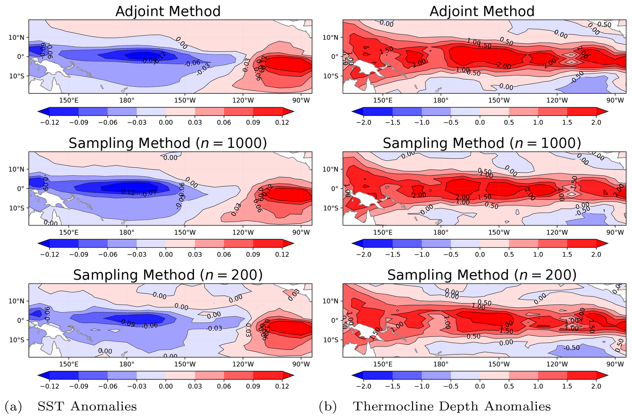
Figure 1 The spatial patterns of the optimal precursors in terms of SST anomalies (a) and thermocline depth anomalies (b). The prediction time is 9 months. By the rows from top to bottom, the spatial patterns are obtained by the adjoint method, the sampling method with n=1000, and the method with n=200, respectively.

3.1 Optimal precursors in the ZC model

Recall the optimal precursors bringing about the El Niño event, which is obtained by the CNOP approach in Yu et al. (2009). The spatial pattern in terms of SST anomalies is manifested as a large-scale zonal dipolar pattern, the warm pole of about 0.2 °C along the Equator in the east Pacific, and the cold one of about 0.2 °C in the central Pacific, while a basin-side deepening about 100 m along the Equator is the character of that for thermocline depth anomalies. We reproduce the spatial patterns of the optimal precursors bringing about the El Niño event in Fig. 1, the two pictures in the top row. When we take 1000 samples to implement the sampling method, both the spatial patterns of the optimal precursors in terms of SST anomalies and thermocline depth anomalies are almost identical to those obtained by the adjoint method, shown in the middle row of Fig. 1. Furthermore, when the number of samples is reduced from 1000 to 200, we can find from the two pictures in the bottom row of Fig. 1 that both the large-scale zonal dipolar pattern of SST anomalies and the basin-side deepening pattern of thermocline depth anomalies for the optimal precursors leading to the El Niño event can be still captured, even though there are some small deviations due to some noise.

Table 1 The optimal precursors u₀ are computed by both the adjoint method and the sampling method, with the corresponding spatial patterns shown in Fig. 1. First line: the objective values J(u₀) computed in Eq. (4). Second line: the percentages over the values computed by the adjoint method. Bold highlights the high efficiency of the sampling method with n=200.

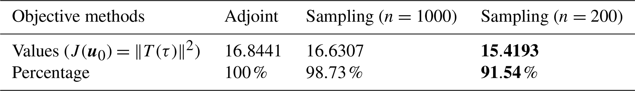
We have shown considerable similarities in the spatial patterns of the optimal precursors bringing about the El Niño event in Fig. 1, which are obtained by the adjoint method, the sampling method with n=1000, and the method with n=200. If these can be viewed as qualitative similarities, we still need to verify the similarities of the optimal precursors from these numerical algorithms quantitatively. The objective values J(u₀) obtained using the optimal precursors u₀ computed by both the adjoint method and the sampling method are shown in Table 1, where we can find that the value computed by the adjoint method is 16.8441, and the values by the sampling method with n=1000 and n=200 are 16.6307 and 15.4193, respectively. The objective values obtained by the sampling algorithm look very close to the one of the baseline adjoint method. Here, we can further show the similarities by taking the ratio between them. If the objective value obtained by the adjoint method is taken as the numerator, we can find that the objective value obtained by the sampling method with n=1000 takes the percentage 98.73 %, which shows that the objective values obtained by the two algorithms are almost identical. When the number of samples is reduced from 1000 to 200, the percentage that the objective value obtained by the sampling algorithm occupies decreases to 91.54 %, which is still more than 90 % and shows quite high similarities.

Both the spatial patterns and the objective values indicate that the optimal precursor obtained through the sampling algorithm, using only 200 samples, is very similar to the one obtained through the baseline adjoint algorithm. To show the efficiency of the sampling method, a comparison of computation times is necessary. As mentioned in Sect. 2.2, the sampling algorithm, implemented with parallel computation, reduces the computation of the gradient by performing a single forward numerical integration. In contrast, the adjoint method requires a two-step process involving both forward and backward numerical integrations. We have realized them and recorded the computation times of both the adjoint method and the sampling algorithm implemented with parallel computation in Table 2.

Table 2 The comparison of computation times between the adjoint method and the sampling method under the parallel computation. The Fortran code was run on the following CPU: Intel^® Xeon^® Gold 6132 Processor, 19.25M Cache, 2.60 GHz, with eight nodes and 28 cores per node.

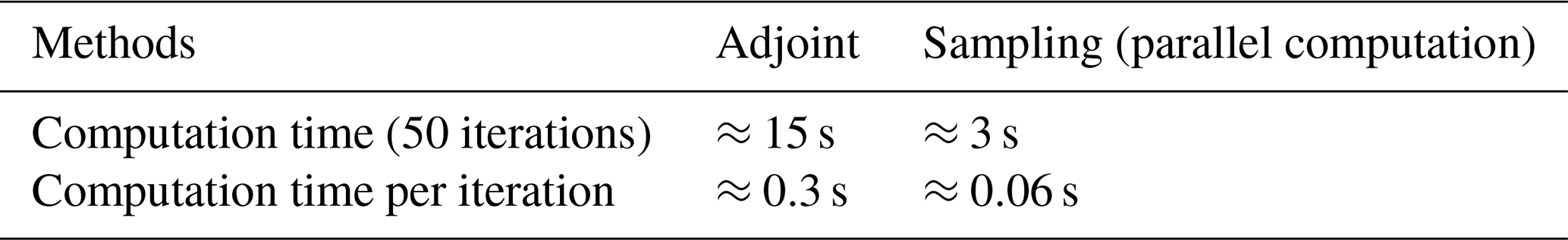
It needs to take about 50 iterations by implementing both the adjoint method and the sampling method to get the optimal precursors. On the supercomputer, the adjoint method takes about 15 s (that is, about 0.3 s per iteration), while the sampling method takes about 3 s when the implementation is under the parallel computation (that is, about 0.06 s per iteration). Furthermore, when the sampling method is implemented, we avoid running the numerical model reversely such that the computation time is shortened to $\mathrm{1}/\mathrm{5}$. Without any doubt, the computation that is reduced must be implemented by parallel computation. However, based on the current resource of computation, it is available for us to implement the sampling method under the parallel computation to obtain the optimal precursors by the use of the CNOP approach in the ZC model and, more generally, the numerical model with a number O(10⁴−10⁵) of degrees of freedom.

3.2 Nonlinear time evolution behavior of the optimal precursors

Based on the CNOP approach, the statically spatial patterns of the optimal precursors of ENSO events are in terms of both SST anomalies and thermocline depth anomalies. In Sect. 3.1, we showed the high efficiency of the sampling algorithm by the comparison with that obtained by the baseline adjoint method as well as the computation times. However, we still need to study the dynamic behaviors of the ENSO events to predict the potential impacts, where a great way is to only monitor the nonlinear evolution of SST anomalies.

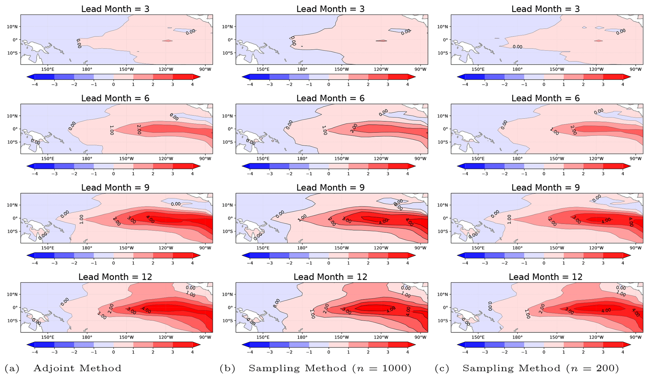
Figure 2 The spatial patterns of the nonlinear time evolution of the optimal precursors in terms of SST anomalies.

Recall the nonlinear time evolution of SST anomalies simulated by the coupled ocean–atmosphere ZC model shown in Yu et al. (2009), where the optimal precursor, or CNOP, is obtained by the adjoint method. By adding the initial optimal precursors to the climatological mean equilibrium state, we run the ZC model to reproduce the EP-type El Niño phenomenon in the left column of Fig. 2, where we observe that the warm phase in the east Pacific along the Equator is intensified gradually with the season evolution in 1 year; that is, the lead time is set as 3, 6, 9, and 12 months, respectively. More concretely, in the east Pacific along the Equator, the region of the warm phase is gradually enlarged and the SST anomalies are raised up sharply from about 0 to 8 °C. In the right two columns of Fig. 2, we show the spatial patterns in terms of the nonlinear time evolution of SST anomalies, where the initial condition starts from the climatological mean equilibrium state added by the initial optimal precursors obtained by the sampling methods with n=1000 and n=200. By taking a comparison between the spatial patterns shown from the left to the right in Fig. 2, the nonlinear time evolution behaviors of the initial optimal precursors are also remarkably similar to each other with the change of seasons. Even though the number of samples is reduced to 200, we still find that the spatial patterns in terms of the seasonal evolution of SST anomalies are almost consistent with the baseline pattern, starting from initial optimal precursors obtained by the adjoint method.

Based on the nonlinear time evolution of SST anomalies simulated in Fig. 2, we have qualitatively shown the similarities of the dynamical behaviors of the initial optimal precursors obtained by both the baseline adjoint method and the sampling method. Nevertheless, we still need to show the similarities quantitatively for the dynamical evolution of SST anomalies from the three kinds of initial optimal precursors.

Currently, the main variable that is considered from the ENSO forecasts of the coupled climate models is the Niño 3.4 SST anomaly index, which is used by the National Climate Centre (NCC) in Australia to classify ENSO conditions. Here, we show that the Niño 3.4 SST anomaly indices change nonlinearly along the time evolution line within a model year in Fig. 3, where the three dynamical curves generated by these proposed algorithms are quite close to each other. Furthermore, we can observe in Fig. 3 that the dynamical curve of the Niño 3.4 SST anomaly index starting from the initial optimal precursor obtained by the sampling method with n=1000 almost coincides with the baseline one from the initial optimal precursor obtained by the adjoint method. When the number of samples is reduced from 1000 to 200, some small deviations appear in the dynamical curve of the Niño 3.4 SST anomaly index. Thus, it is necessary for us to quantify these derivations such that we can study the accuracy of the Niño 3.4 SST anomaly index by implementing the sampling algorithm to approximate that generated by the adjoint method when the number of samples is reduced from 1000 to 200. Taking the Niño 3.4 SST anomaly index generated by the adjoint method as a basis, we compute the relative Niño 3.4 SST anomaly index, that is, the difference of the Niño 3.4 SST anomaly indices from between the baseline adjoint method and the sampling method in Fig. 4.

Here, we can find that the relative Niño 3.4 SST anomaly index from the sampling method with n=1000 takes the characteristic scale with O(10⁻²), while that from the sampling method with n=200 is O(10⁻¹). In other words, when we implement the sampling method by reducing the number of samples from n=1000 to n=200, the relative Niño 3.4 SST anomaly index is degraded from O(10⁻²) to O(10⁻¹), which quantitatively manifests that the accuracy of the Niño 3.4 SST anomaly index is loosened up to an order of magnitude. However, if we take the comparison with the Niño 3.4 SST anomaly index, whose characteristic scale is O(1), the numerical errors by reducing the number of samples from 1000 to 200 are still too small to influence the nonlinear time evolution of SST anomalies.

4 Summary and discussion

Based on state-of-the-art statistical machine learning techniques, the sampling method to compute CNOPs is proposed in Shi and Sun (2023). In this paper, we successfully implement the sampling method to obtain the initial optimal precursors in the realistic and predictive ZC model and, more generally, the numerical model with a number O(10⁴−10⁵) of degrees of freedom. The sampling method with fewer samples can achieve consistent performance with the adjoint method in the numerical experiments, regardless of the statically spatial patterns and the dynamical nonlinear time evolution behaviors, as well as the corresponding quantities and indices. By leveraging the key characteristic that the samples are independently and identically distributed, we can effectively implement the sampling method using the modern parallel computation technique. This approach eliminates the need to run the numerical model in reverse, leading to a significant reduction in computation time. In fact, the computation time can be shortened by approximately $\mathrm{1}/\mathrm{5}$, allowing for more efficient and faster processing. In general, the number of samples required for a numerical model depends on the degrees of freedom. As the degrees of freedom increase, a larger number of samples is typically needed. However, the nonlinear evolution of the initial values within the numerical model itself should not be overlooked. This has been empirically demonstrated in a comparison between the Burgers equation and the Lorenz-96 model (Shi and Sun, 2023). In the case of the Burgers equation, which exhibits weak nonlinear evolution, achieving the desired experimental effect can be accomplished with just five samples, even with 100 degrees of freedom. On the other hand, the 40-dimensional Lorenz-96 model, characterized by strong nonlinear evolution, also requires five samples to achieve the desired effect. Based on empirical observations, a good strategy for initial experiments is to choose the number of samples to be approximately equal to the square root of the number of degrees of freedom, that is, $n\approx \sqrt{d}$. Indeed, by implementing the sampling algorithm with 60 samples, we are able to achieve a numerical performance that nearly reproduces the results obtained by the baseline adjoint method for the optimal precursors. However, it has been observed that the numerical results are unstable. Out of four runs, only one consistently produces correct numerical performance. In addition, by the use of the CNOP approach in the coupled ocean–atmosphere ZC model, we can obtain another kind of optimal precursors which lead to the La Niña event. However, due to the deficiency of the original ZC model in Zebiak and Cane (1987), a warm tendency of the Niño 3.4 SST anomaly index will appear after it decreases to the coldest point for the La Niña event, which is shown in Duan et al. (2008). In our numerical experiments, the numerical performance based on the optimal precursors leading to the La Niña event can also be obtained. Thus, these numerical experiments are not representative, so we neglect to show their numerical performance in the paper.

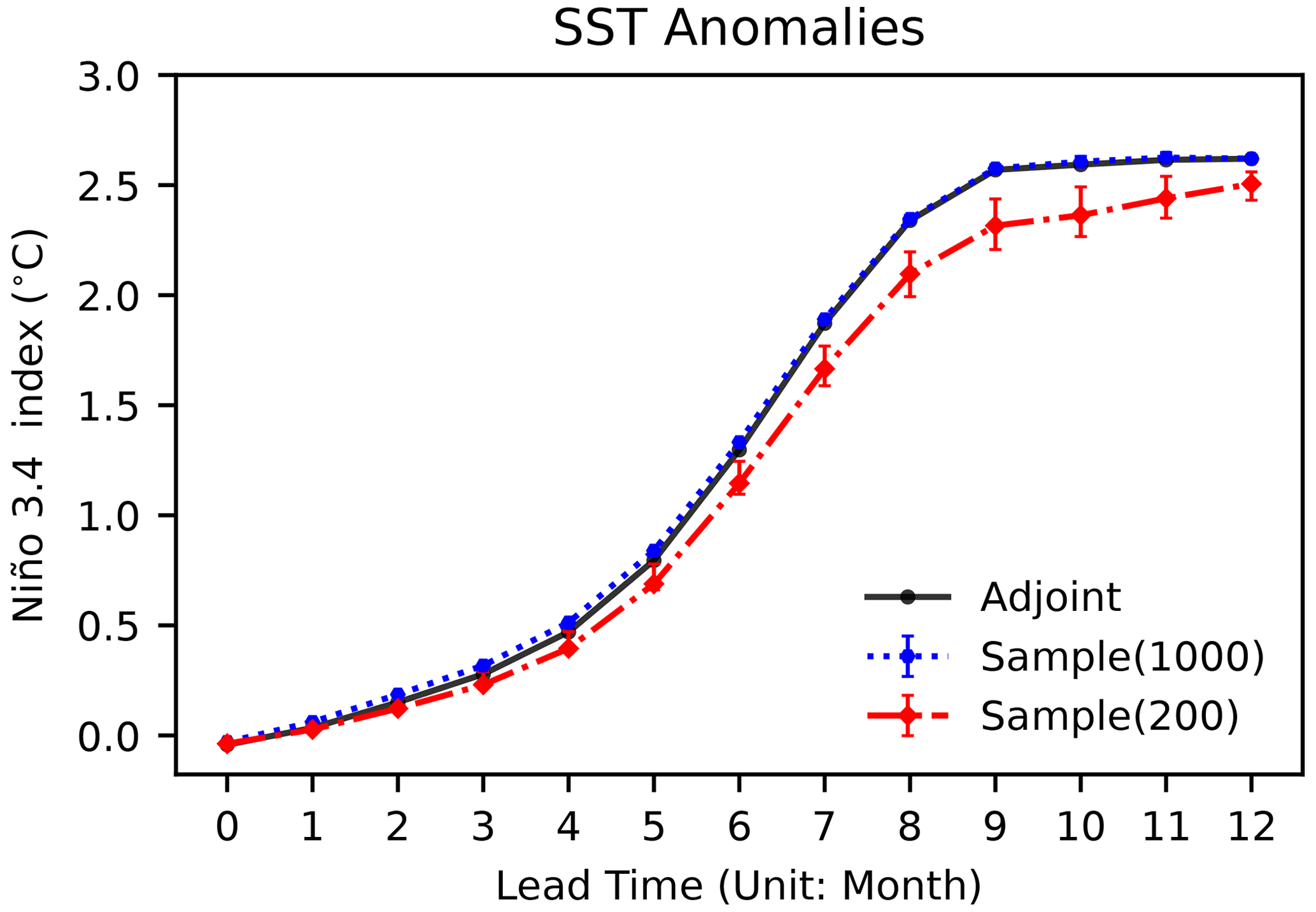
Figure 3 The nonlinear time evolution of the Niño 3.4 SST anomaly index within a model year. The bars represent the range of errors obtained from running the sampling method 50 times.

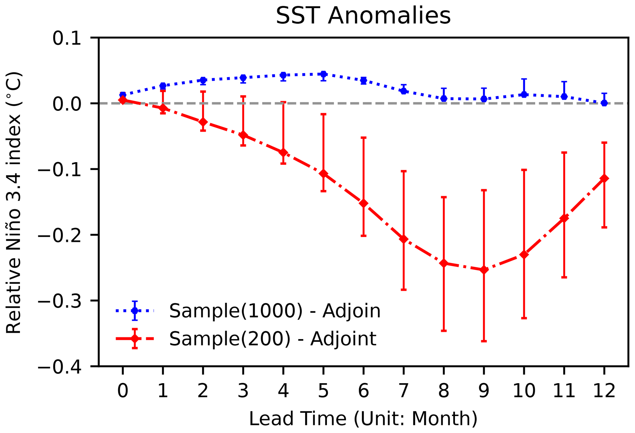
Figure 4 The nonlinear time evolution of relative Niño 3.4 SST anomaly index within a model year (the Niño 3.4 SST anomaly index obtained by the sampling method minus that by the baseline adjoint method). The bars represent the range of errors obtained from running the sampling method 50 times.

For a realistic global climate system model (GSCM) or atmosphere–ocean general circulation model (AOGCM), it is often impractical to develop the adjoint model, so the sampling method provides a probable way of computing CNOPs to investigate its predictability. An interesting direction for further research is to investigate CNOPs computed by the sampling method in the numerical models that are used in realistic prediction and forecast, such as the Weather Research and Forecasting (WRF) model, a state-of-the-art mesoscale numerical weather prediction system for operational forecasting applications. Another interesting direction is to attempt to use the sampling method to realize a more (or less) nonlinearly stable flow by changing some aspect of the system (Cherubini and De Palma, 2013; Rabin et al., 2014; Passaggia and Ehrenstein, 2013), where the adjoint technique still needs to make costly optimization calculations (Kerswell, 2018). In addition, the traditional data assimilation is based on the development of the adjoint model (Kalnay, 2003). In this paper, our numerical experiments allow the four-dimensional variational (4D-Var) data assimilation technique to become available for the coupled climate system models as well as the parameterization models. Therefore, it is valuable and thrilling to implement the sampling method to process 4D-Var data assimilation in realistic systems, such as the Flexible Global Ocean-Atmosphere-Land System (FGOALS)-s2 (Wu et al., 2018) for decadal climate prediction. Finally, we conclude this paper with a statement that the sampling method, based on state-of-the-art machine learning techniques, is a probable way to realize the nonlinear optimization method in practice to address these challenges in Kerswell (2018) and Wang et al. (2020).