the Creative Commons Attribution 4.0 License.
the Creative Commons Attribution 4.0 License.
 | 08 Dec 2023
Uncertainties, complexities and possible forecasting of Volcán de Colima energy emissions (Mexico, years 2013–2015) based on a fractal reconstruction theorem
Marisol Monterrubio-Velasco
Xavier Lana
Raúl Arámbula-Mendoza
The effusive–explosive energy emission process in a volcano is a dynamic and complex physical phenomenon. The importance of quantifying this complexity in terms of the physical and mathematical mechanisms that govern these emissions should be a requirement for deciding to apply a possible forecasting strategy with a sufficient degree of certainty. The complexity of this process is determined in this research by means of the reconstruction theorem and statistical procedures applied to the effusive–explosive volcanic energy emissions corresponding to the activity in the Volcán de Colima (western segment of the Trans-Mexican Volcanic Belt) along the years 2013–2015. The analysis is focused on measuring the degree of persistence or randomness of the series, the degree of predictability of energy emissions, and the quantification of the degree of complexity and “memory loss” of the physical mechanism throughout an episode of volcanic emissions. The results indicate that the analysed time series depict a high degree of persistence and low memory loss, making the mentioned effusive–explosive volcanic emission structure a candidate for successfully applying a forecasting strategy.
- Article
(2801 KB) - Full-text XML
- BibTeX
- EndNote


Right forecasting of dangerous long drought episodes, high-magnitude earthquakes or great volcanic emissions should be one of the main objectives of the scientific fields of climatology, seismology or volcanology to prevent disasters which could affect the environment and human life. Several examples of forecasting algorithms could be cited, among them the nowcasting strategy (Rundle et al., 2016, 2017), the multi-fractal analysis in seismology (Monterrubio-Velasco et al., 2020), the ARIMA (auto-regressive integrated moving average based on a reconstruction theorem) process in climatic research (Lana et al., 2021) and neural algorithms (Lipton et al., 2015; Lei, 2021), which are also useful for predicting monthly rainfall. These cited algorithms systematically forecast the next episode, taking into account a certain number of previously recorded data, this number being strongly associated with the characteristics of the physical mechanism. These forecasting results should be validated by previously analysing the degree of complexity and the “loss of memory” of the physical mechanisms along the evolution of the physical process. In other words, how many previous data would be necessary for right use of a forecasting algorithm, and what could the range of uncertainties in the predictions be?
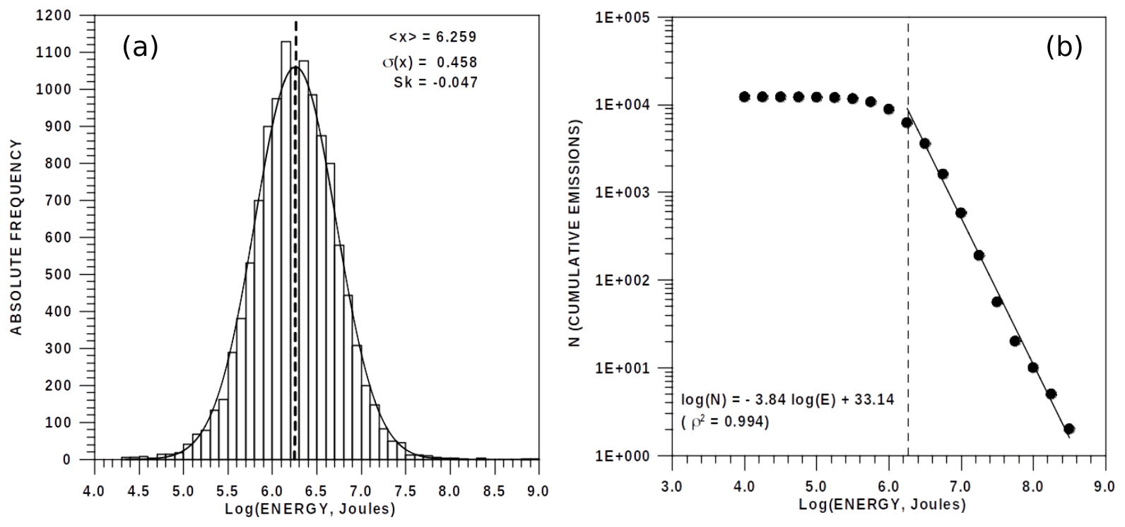
Figure 1(a) Histogram of the volcanic emission energies and (b) logarithm of energies fulfilling the Gutenberg–Richter law.
The database, analysed in this research in Sect. 2, is the time series of explosive volcanic events (Vulcanian explosions) emitted by the Volcán de Colima (western segment of the Trans-Mexican Volcanic Belt) during the years 2013–2015. A Vulcanian explosion is an eruption where fragmented material is expelled into the atmosphere as a result of overpressure into the conduit or lava dome (Arámbula-Mendoza et al., 2018). The event releases energy in several ways based on elastic, seismic, acoustic and thermal processes. The next explosion will occur when the overpressure breaks the impermeable cap again. The Volcán de Colima has emitted many Vulcanian explosions, some of them with generation of pyroclastic density currents (PDCs) until 5 km of runout (Arámbula-Mendoza et al., 2019). For these reasons, strategies for right forecasting of the mentioned Vulcanian explosions are important.
The reconstruction theorem (Sect. 3) is a mathematical strategy that allows quantification of the degree of complexity in a time series and its loss of memory, which are both required to validate a possible forecasting strategy (Diks, 1999). Additionally, the nowcasting algorithm (Sect. 5), a statistical process developed by Rundle et al. (2016, 2017) to detect the risk of imminent high-magnitude earthquakes, could also be applied to quantify the probability of an imminent high-magnitude volcanic emission.
The main objective of this work is to detect the degree of difficulty for a forecasting of volcanic emissions associated with energies close to or exceeding 108 J. By means of the reconstruction theory (Diks, 1999), the complexity is measured by means of some parameters such as the persistence degree, the intensity of the chaotic behaviour of the system and the loss of memory of the physical mechanism. Moreover, the statistical distributions of the effusive–explosive energy of these emissions and their return periods are also analysed. The just-mentioned nowcasting strategy is also taken into account to confirm future extreme emissions of energy. The results obtained after applying the reconstruction theorem and analysing the whole time series, six consecutive segments and 21 moving window data are detailed in Sect. 4.
The most relevant results of the reconstruction theorem and their effects on forecasting algorithms are discussed in Sect. 6. Finally, Sect. 7 (“Conclusions”) summarises the most relevant results with respect to the expected success in preventing volcanic energy emissions based on forecasting and nowcasting processes.
A time series of volcanic explosions, named Vulcanian explosions (Clarke et al., 2015), emitted by the Volcán de Colima (western segment of the Trans-Mexican Volcanic Belt, years 2013–2015) (Arámbula-Mendoza et al., 2018) is analysed. Figure 1a depicts the histogram of the logarithm of the emitted energy. The dataset contains 6182 observations of the emissions equalling or exceeding approximately 2×10⁶ J, fulfilling the Gutenberg–Richter law (Gutenberg and Richter, 1956), as shown in Fig. 1b.
Figure 2a describes the six segments to be analysed with 1000 samples and a seventh segment that is excluded from the analysis due to a lack of data. The highest explosions can be observed at the beginning of the first segment [log10(Energy)=8.2], third segment [log10(Energy)=8.4] and end of the series in the seventh segment [log10(Energy)=8.9]. With the aim of analysing the whole set of volcanic emissions fulfilling the Gutenberg–Richter law, Fig. 2b depicts two examples of moving window segments.
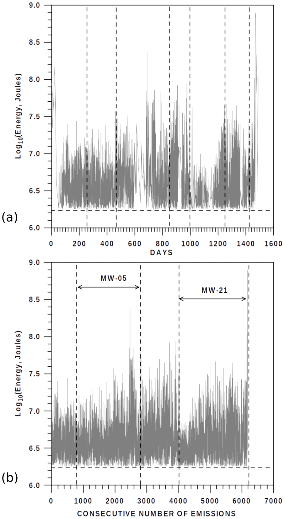
Figure 2(a) Evolution of the volcanic energy emission fulfilling the Gutenberg–Richter law. Vertical dashed lines define the segments (intervals of 1000 data). (b) Two examples of a dataset defined by moving windows of amplitude 2 1000 elements and shifting 200 positions.
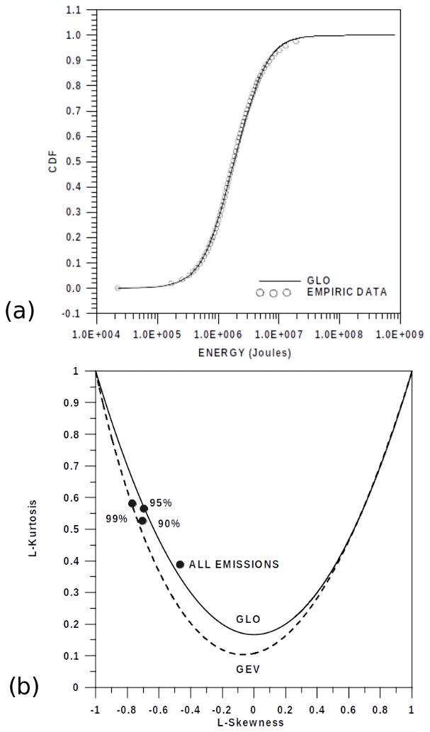
Figure 3(a) Cumulated distribution function of the effusive volcanic energy emissions, well fitted to the GLO (generalised logistic distribution). (b) The emissions equalling or exceeding 90 %, 95 % and 99 % could be associated with the GEV (generalised extreme value distribution), in agreement with the L-skewness or L-kurtosis diagram. The theoretical cumulated distribution GLO of the volcanic emissions is also confirmed by means of the mentioned diagram.
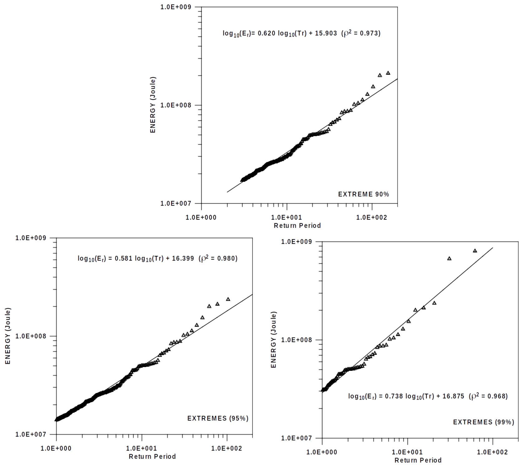
The statistical distribution of these emissions is analysed by means of the L-skewness or L-kurtosis formulation (Hosking and Wallis, 1997). The statistical analysis of these emissions shows that the complete series of emissions, including those not fulfilling the Gutenberg–Richter law, are well fitted to the generalised logistic, GL, function (Fig. 3a and b). Additionally, three different empirical distributions of extreme emissions, equalling or exceeding 90 %, 95 % and 99 % respectively of the data (Fig. 3b), can be associated with the generalised extreme value, GEV, function. Figure 4 shows the evolution of these three expected extreme emissions with the increasing return periods (given as the number of events equalling or exceeding 90 %, 95 % and 99 % respectively). For instance, the expected values of emissions for the three percentage levels and return periods with up to 200 extreme emissions fit the theoretical evolution quite well, with emissions close to 1.0×10⁸, 2.0×10⁸ and 8.0×10⁸ J for the 90 %, 95 % and 99 % extreme distributions. This first approach to the possibility of very high explosions and the corresponding expected return period (number of extreme episodes before a very high extreme emission) would be quite similar to a nowcasting analysis, a strategy proposed by Rundle et al. (2016, 2017) to detect the risk of imminent high-magnitude earthquakes.
Prior to the reconstruction theorem (Diks, 1999) based on monofractal theory, the degree of randomness, anti-persistence or persistence of the analysed data is established by taking into account the concept of the Hurst exponent (Turcotte, 1997), which is defined as the exponent H of the power law.
R(τ) is the range of the different chosen segments of length τ of a series and S(τ) is the corresponding standard deviation. H close to 0.5 implies a strong randomness of the series. Conversely, H clearly lower than or exceeding 0.5 means anti-persistence or persistence, respectively. Consequently, the Hurst exponent offers a first point of view of the behaviour of the analysed series. It should also be remembered that the Hurst exponent has to be coincident with a specific value of the generalised Hurst exponent, obtained by means of multi-fractal analysis (Kantelhardt et al., 2002) applied to the same series.
The analysis of the monofractal structure of a series, by means of the reconstruction theorem (Diks, 1999), permits quantification of its complex forecasting by means of the following parameters.
-
The necessary minimum number of non-linear equations governing the physical mechanism, usually referenced as a correlation dimension μ(m), m being the reconstruction space dimension
-
The embedding dimension, dE, the asymptotic value of the correlation dimension, with m theoretically tending to ∞
-
The Kolmogorov entropy, k, which quantifies the loss of memory of the mechanism along the analysed physical process
The reconstruction theorem process is based on generating a set of m-dimensional space vectors using the series {x(i)} of data.
n is the length of the series, and the definition of the correlation integral in terms of the Grassberger–Procaccia formulation (Grassberger and Procaccia, 1983a, b) is
r is a Euclidean distance in the m-dimensional space and H{.} is a Heaviside function. The correlation integral can be rewritten as
K is the Kolmogorov entropy exponent, and Am and μ(m) are the correlation amplitude and the mentioned correlation dimension for every reconstruction dimension m. A confident quantification of μ(m) for every reconstruction dimension has to be carefully computed, avoiding a very flat evolution of C(m,r) for small values of r caused by the lacunarity (Turcotte, 1997) and the saturation of C(m,r) for the highest values of r. With respect to the quantification of the Kolmogorov entropy, K, by using Eq. (5), naming μ(m) the term and after obtaining α(m), Eq. (5) becomes
Equation (6) is characterised by an almost constant value of log (Am) for high reconstruction dimensions m. Consequently, a very accurate value of the Kolmogorov coefficient K could be obtained by a linear regression in terms of Eq. (6), but only for the mentioned set of the highest reconstruction dimensions m. The same set of m-dimensional space vectors permits the computation of the Lyapunov exponents λi () (Eckmann et al., 1986; Stoop and Meier, 1988; Wiggins and Zeidler, 1991), which quantify the intensity of the chaotic behaviour of a system, especially the first λ1 exponent when the results, forthcoming volcanic emissions in the present case, are estimated by means of some forecasting algorithm. Additionally, the Kaplan–Yorke dimension, DKY (Kaplan and Yorke, 1979), is
with l0 the maximum number of Lyapunov exponents in decreasing order fulfilling
This quantifies the fractal dimension of the nucleus around which the consecutive m-dimensional vectors describe the corresponding orbital trajectories. In short, the higher the value of DKY is, the more complex it will be to establish the forthcoming value of the analysed physical problem.
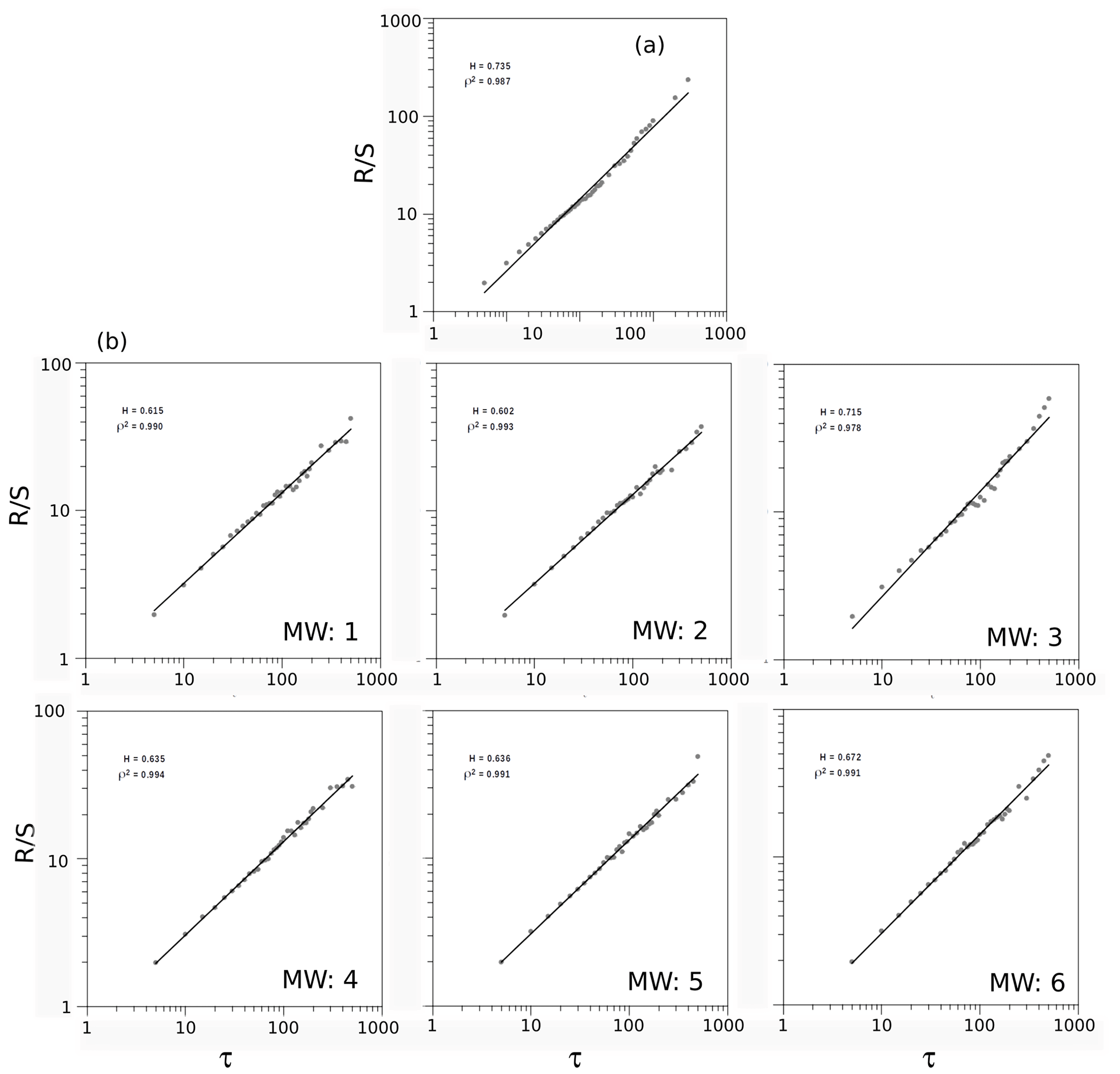
Figure 5Some examples of the Hurst exponent for (a) the whole series of effusive emissions of energy fulfilling the Gutenberg–Richter law and (b) the same series fragmented on six trams of an equal number of records. In agreement with the definition of Eq. (1), has no units and τ represents the different lengths (number of data) of the segments considered.
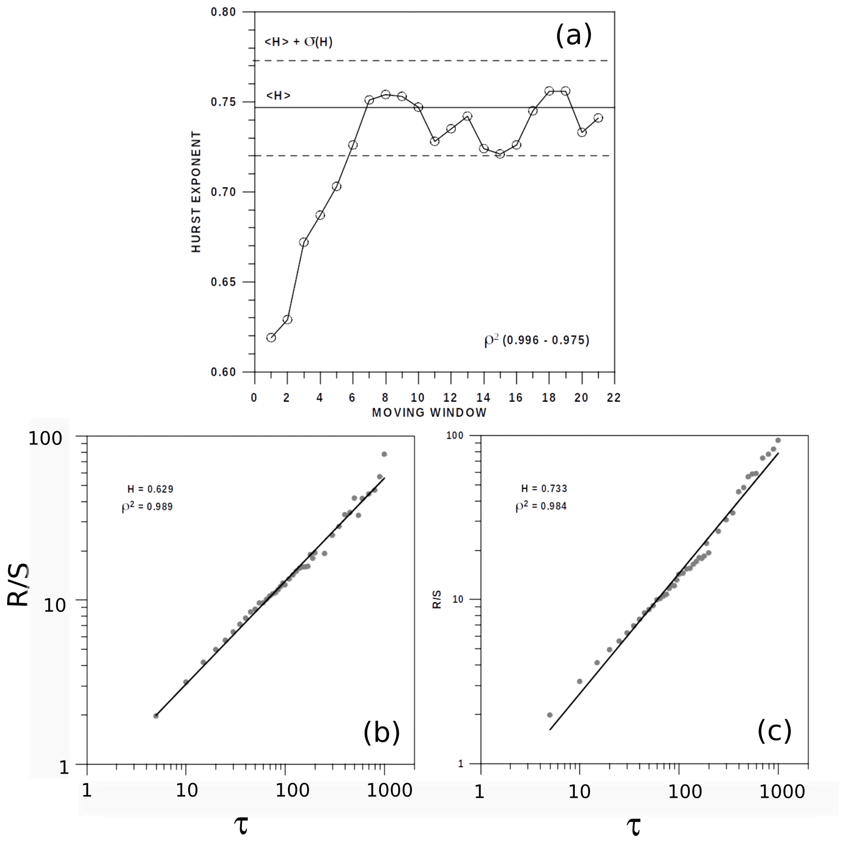
Figure 6(a) Evolution of the Hurst exponent for the 21 moving windows and two examples for windows (b) 2 and (c) 6.
4.1 The Hurst exponent
The results of the Hurst exponent for the whole series and the six data segments are described in Fig. 5a and b, obtaining a clear sign of persistence for the complete series of Vulcanian explosions, with H exceeding a value of 0.7; a moderate persistence for the first, second, fourth and fifth segments; a smooth increase in H from the fifth to sixth segments; and a clear persistence (H>0.70) for the third segment. This third clear persistence is detected for a data segment including the second-highest energy emission (Fig. 2a and b). Conversely, the lowest Hurst exponents for the first, second, fourth and fifth segments are characterised by more moderate emissions of energy. Finally, the increase in H for the sixth segment could be caused by the imminence of the highest energy, an emission immediately after this data segment. A more detailed evolution of the Hurst exponent is described by the 21 moving windows (Fig. 6a and b), detecting that the increase in the persistence for the first six moving windows is stabilised for the other 15 windows with notable signs of persistence, with H varying from 0.72 to 0.76. In short, the factor of persistence from the point of view of the Hurst exponent suggests a certain facility of forecasting algorithms. It is remarkable that, after the first 1000 emissions (beginning of the five moving windows), the highest persistency with some fluctuations is achieved and the highest emissions are included in these windows.
Table 1Embedding dimension and Kolmogorov coefficient for the 21 moving windows.
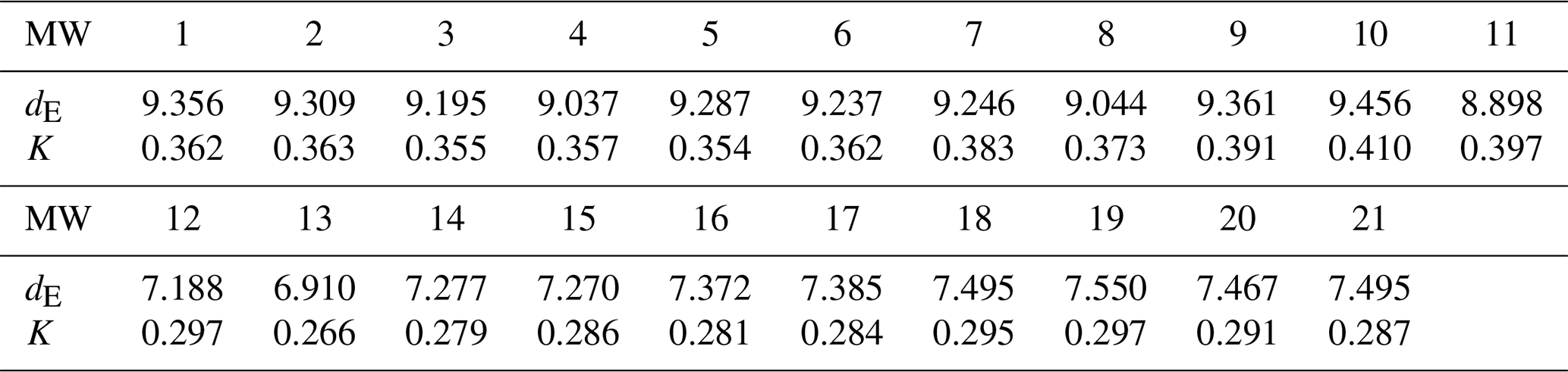
Table 2Embedding dimension and Kolmogorov coefficient for the six segments of volcanic emissions.
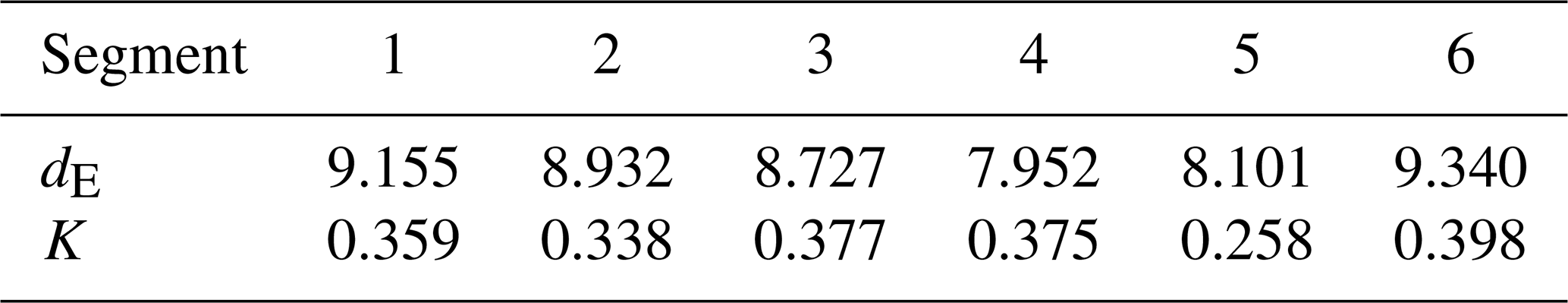
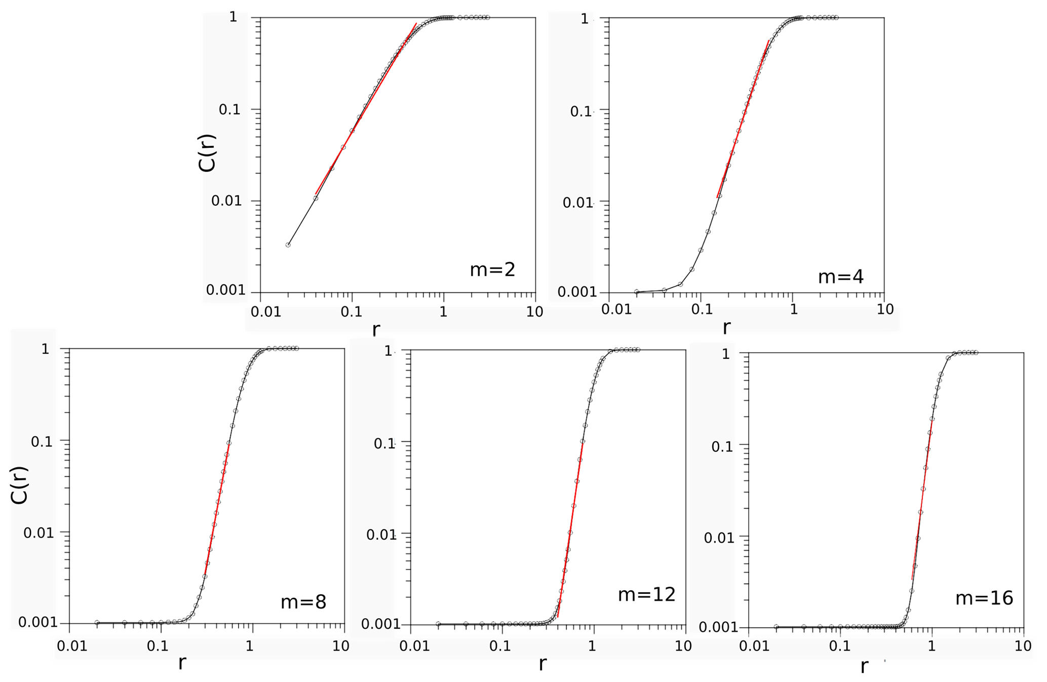
Figure 7An example of the evolution of embedding dimensions (first segment of 1000 elements) for reconstruction dimensions m=2, 4, 8, 12, and 16. The straight red line represents the interval of r values that can be determined for every one of the embedding dimensions.
4.2 Embedding dimension
With respect to the embedding dimension, Fig. 7 illustrates five examples of the first segment of 1000 recorded emissions, where the slope, μ(m), of log10{C(r)} with respect to log10{r} monotonically increases for an interval of r, which then describes the asymptotic evolution of these slopes towards the definitive embedding dimension dE. The embedding dimensions for the 21 moving windows and the six segments are respectively summarised in Tables 1 and 2. By remembering that this dimension defines the minimum number of non-linear differential equations associated with the physical process, the most complex segments from a mathematical point of view would be the first, second, third and sixth ones, which are not as complex as the fourth and fifth ones. Nevertheless, the discrepancies when comparing the different segments are not excessive, given that 9 or 10 differential equations would be sufficient to analyse every one of the six segments. A quite different evolution of dE is obtained for the 21 moving windows (Table 1), with dimensions approximately varying from 9.5 to 6.9. Between the 11th and 13th moving windows, dE diminishes (a more simplified mathematical structure should be assumed for these volcanic emissions), and for the remaining windows (14th–21th), their mathematical structures' complexities return to moderate values (7.3–7.6).
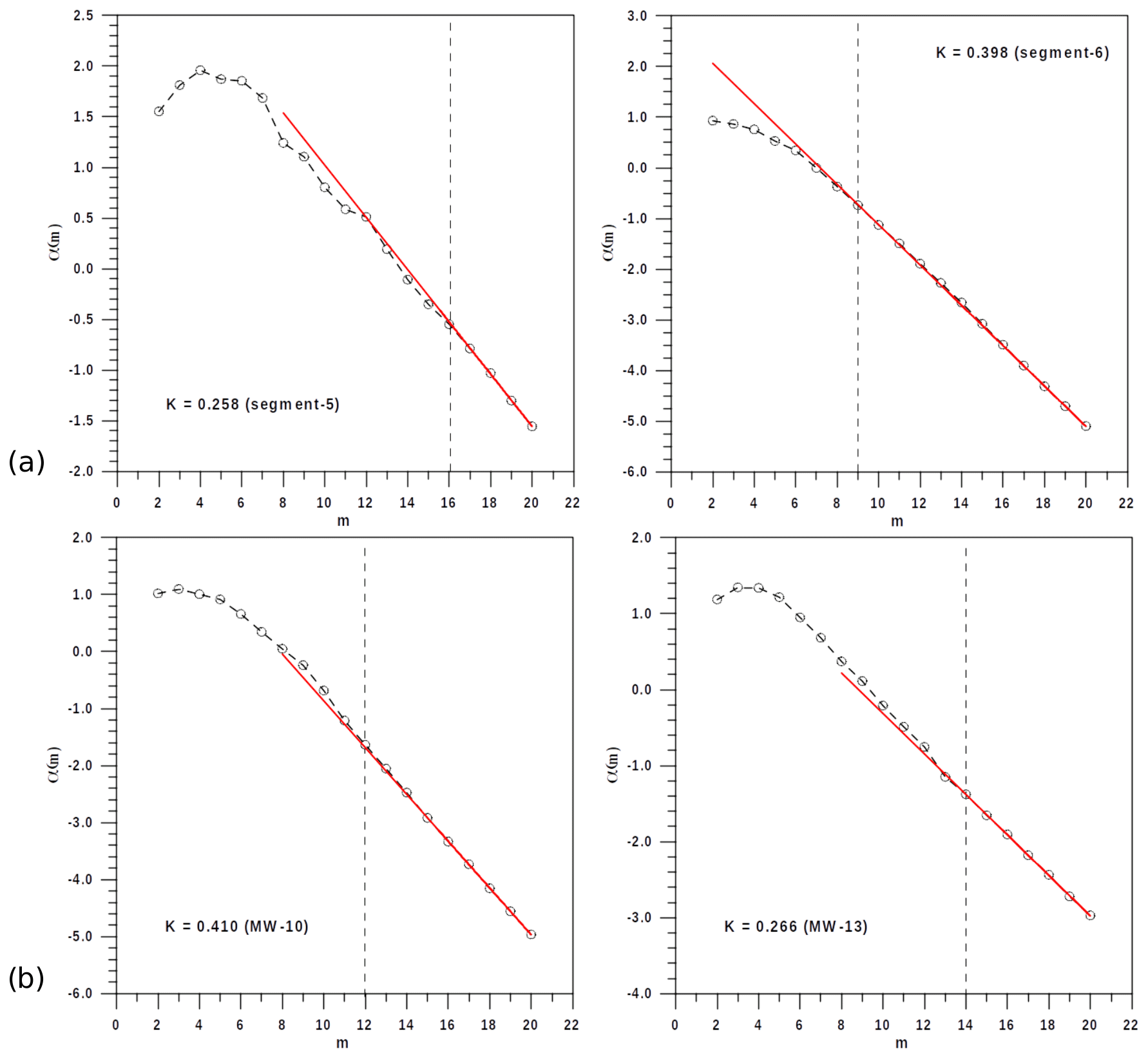
Figure 8(a) Two examples of Kolmogorov entropy exponents, K, for two segments of 1000 elements and (b) for two examples of moving windows. The vertical dashed lines define the parameter m interval used to determine the Kolmogorov entropy for every data segment or moving window.
4.3 The Kolmogorov entropy
The obtained values of the Kolmogorov entropy exponent, based on Eq. (6) and summarised in Tables 1 and 2, are also illustrated with some examples (Fig. 8). In these four examples, the loss of memory of the physical mechanism is quite similar for the 6th segment and the 10th moving window, with values of K which could complicate the forecasting processes a bit more in comparison with the previous 5th segment and the 13th moving window. In spite of these discrepancies with respect to the loss of memory for the different segments and moving windows, they are quite similar in many cases, and there are only two remarkable examples of an extreme minimum (fifth segment, K=0.258) and an extreme maximum (10th moving window, K=0.410). Consequently, the loss of memory, making the forecasting process complex, would not affect all the volcanic explosive emissions in the same way.
Table 3Mean and standard deviation for the first 10 Lyapunov exponents after 975 iterations.
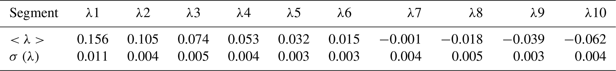
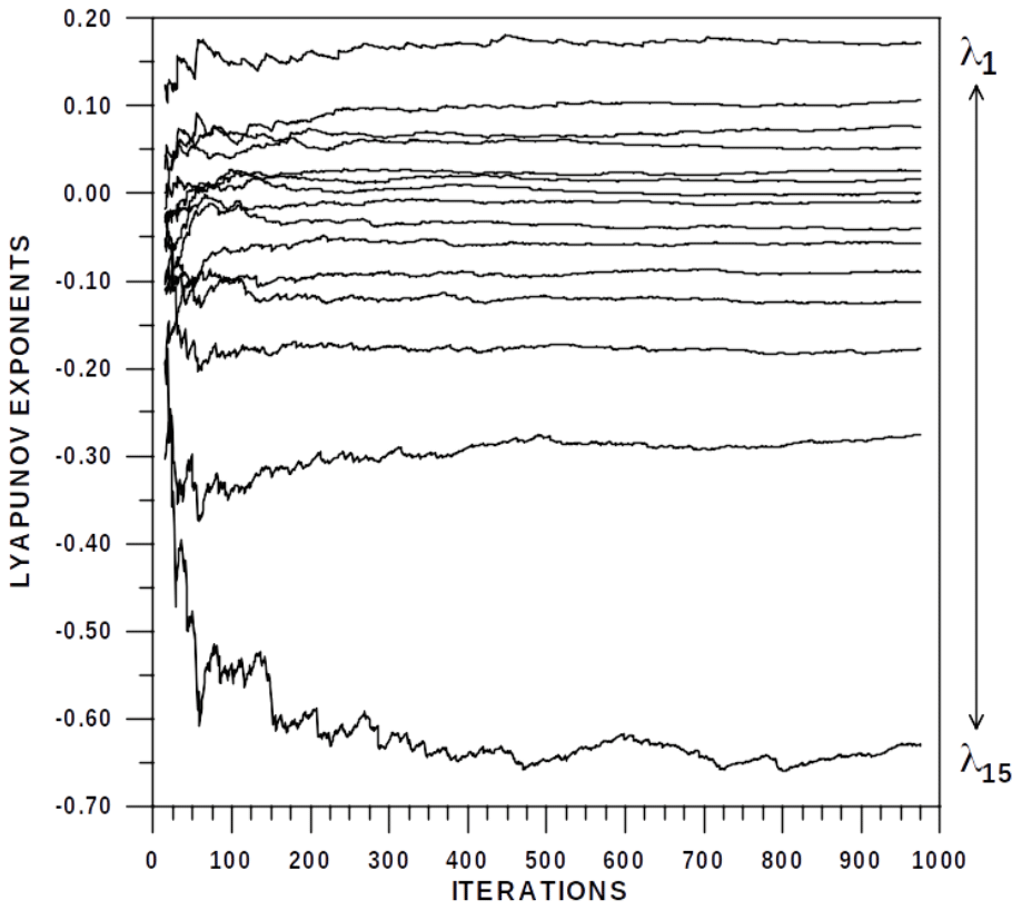
Figure 9Fifteen Lyapunov exponents for the third segment of the effusive–explosive volcanic emissions.
4.4 The Lyapunov exponents
Right computation of the Lyapunov exponents needs an iterative process, with the aim of minimising the final uncertainty on every exponent. In the present computations, 975 iterations have been good enough to obtain the first 15 exponents with very small oscillations at the end of the iterative process. An example of this process is shown in Fig. 9, which describes the evolution of the exponents for the third segment of emissions up to λ15. A higher number of exponents is not necessary for two reasons. First, the possible errors or uncertainties in forecasting processes could be especially associated with the first Lyapunov exponents. Second, observing the evolution at the end of iterations of the exponents of Fig. 9, the Kaplan–Yorke dimension can be computed without the necessity for Lyapunov exponents exceeding dimension 15.
The results are summarised in Table 3, which shows the mean and standard deviation for every one of the first 10 Lyapunov exponents obtained for the 21 moving windows and the six data segments after 975 iterations of the corresponding computational algorithm to obtain accurate and confident values. First, in agreement with the results shown in the mentioned table, every one of the λi exponents is quite similar for both the segments and moving windows, bearing in mind the very similar average values and small standard deviations. Second, the first small negative Lyapunov values are always detected for λ7 or λ8. Consequently, the information offered by the Lyapunov exponents concerning the possible errors in forecasting should be very similar all along the emissions. There are no detected differences between the data segments and the moving windows. Finally, the Kaplan–Yorke dimension manifests a notable similarity for both the segments and moving windows.
While for the six trams, DKY varies from 12.51 to 12.75, the range is quite similar for the 21 moving windows, varying from 12.70 to 13.04. Consequently, the fractal dimension of the nucleus around which the consecutive m-dimensional reconstructed vectors describe the corresponding trajectories is complex (a fractal dimension exceeding 12.0). Nevertheless, this complexity becomes confined within a short interval and is quite similar for all the segments and moving windows.
Table 4Basic characteristics of the energy emissions (logarithm of energy) for the whole database, the six segments of 1000 elements and the last segment of 182 elements. The empirical results of the Kolmogorov–Smirnov, K–S, test are compared with the significance levels of 95 % and 99 %, KS_0.05 and KS_0.01, corresponding to the Gaussian distribution.
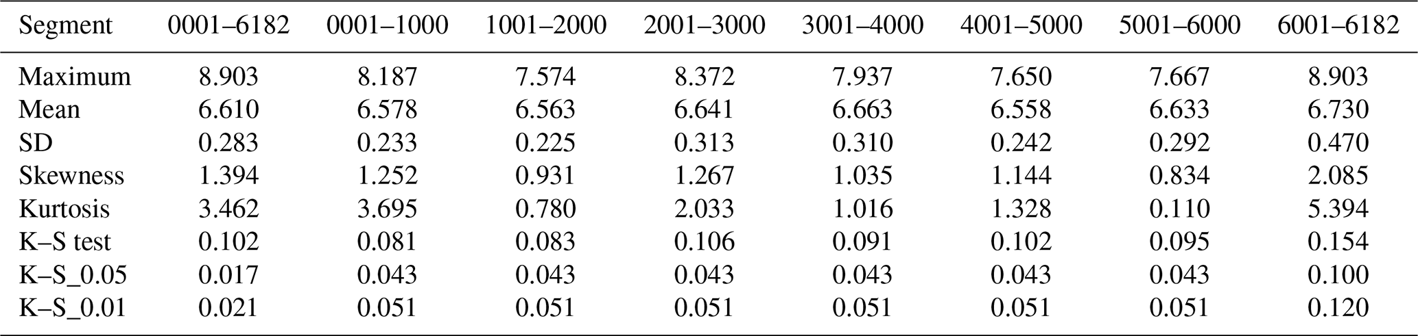
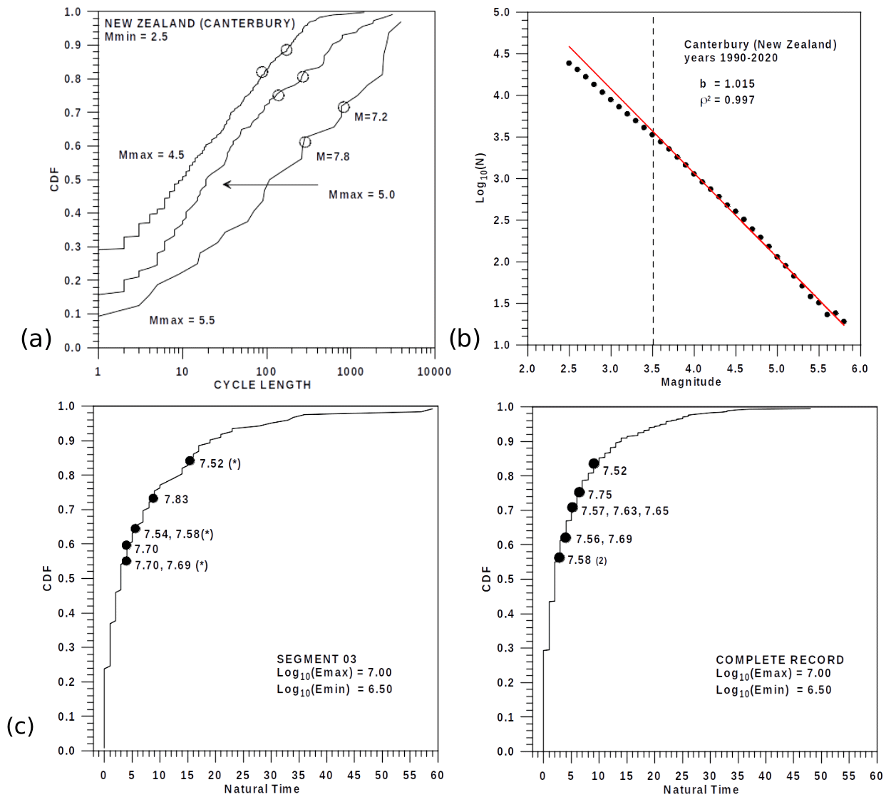
Figure 10A comparison of nowcasting results for (a) the seismic activity of Waitaha / Canterbury (New Zealand), years 1990–2021, and (b) the corresponding Gutenberg–Richter plot and (c) energy of the volcanic emissions of the Volcán de Colima (Mexico), years 2013–2015, bearing in mind Segment 03 of volcanic emissions and (d) the whole volcanic record. The three extreme volcanic records designated by an asterisk (Fig. 10b) are the same as detected in Fig. 10c.
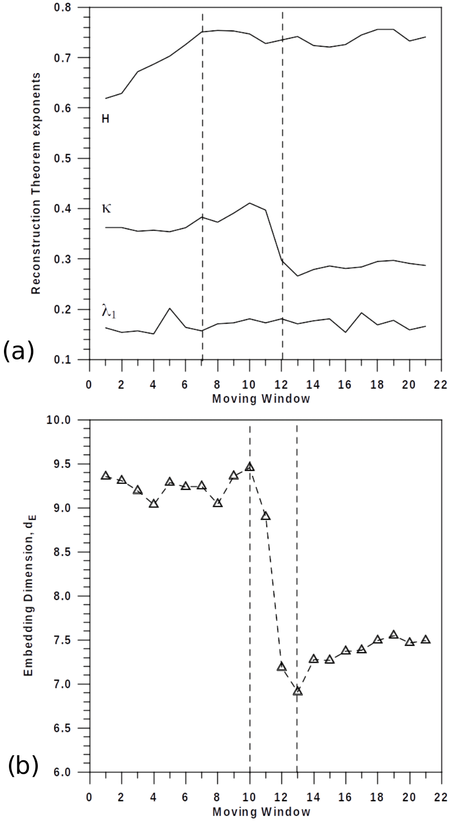
Figure 11(a) Evolution of the Hurst exponent, H, the Kolmogorov entropy exponent, K, and the first Lyapunov exponent, λ1. (b) Embedding dimension dE for the 21 moving windows.
The nowcasting process (Rundle et al., 2016, 2017) is based on the computation of the “natural time” or, in other words, the number of consecutive earthquakes (seismic cycle length) with magnitudes within a determined interval. In this way, the empirical cumulative distribution function, CDF, of these natural times is established by the high-magnitude earthquakes interrupting these seismic cycle lengths. Consequently, the nowcasting process does not exactly predict a forthcoming high magnitude but quantifies the probability of an imminent high earthquake magnitude based on the empirical CDF curves.
A first illustrative example of the nowcasting algorithm, from the point of view of the seismic activity, is depicted in Fig. 10a. It corresponds to the recorded seismic activity in Waitaha / Canterbury (National Earthquake Information Database, https://www.gns.cri.nz, last access: 26 November 2023, years 1990–2020). In spite of the fact that the minimum seismic magnitude fulfilling the Gutenberg–Richter law (Wiemer and Wyss, 2000) should be 3.5 (Fig. 10b), maximum magnitudes of 4.5, 5.0 and 5.5 as well as a minimum magnitude of 2.5 have been considered necessary to obtain a more detailed evolution of the corresponding cycle lengths.
The probability of forthcoming extreme magnitudes (7.2 and 7.8) interrupting a cycle length exceeds 80 %. Consequently, the probability of an earthquake of a similar extreme magnitude should be more or less imminent if the real cycling length ranges between approximately 100 and 1000 natural times, depending on the chosen maximum magnitude Mmax.
Two examples of nowcasting corresponding to volcanic energy explosions are shown in Fig. 10b. The first one corresponds to the volcanic activity of the third segment (Fig. 2a) and the second one includes the whole series of volcanic emissions. In both cases, the cycle lengths are obtained by considering the minimum and maximum levels of volcanic emissions of 102.5 and 104.5 J respectively. Conversely to the example of seismic activity, the few extreme levels exceeding log10(Energy) =8.0 are not associated with high CDF values. Consequently, the nowcasting algorithm could be considered less effective in comparison with the seismic activity results, probably due to the mechanism of the volcanic emissions, which do not include structures such as background activity, swarms, forecasting, mainshocks and aftershocks. Nevertheless, a notable number of high log10(Energy) emissions are slightly smaller than 8.0, and some of them are very close to the highest emissions associated with values of CDFs close to 0.6 and even exceeding 0.8. An example of this fact could be the third segment of emissions, where some of them are not independent but are associated with the highest emission close to 8.5. In short, the nowcasting process could also be assumed to be an algorithm contributing to the predictability of volcanic explosions but perhaps is not as obvious as for the case of seismic activities.
The results obtained by the reconstruction theorem and the possible relationships between the fractal reconstruction exponents (H, K, l and dE) and changes in the volcanic emissions are summarised in Fig. 11a and b. First of all, relevant changes in parameters such as the mean, standard deviation, skewness and kurtosis (Table 4) are not detected for the different segments of volcanic emissions. Additionally, the Kolmogorov–Smirnov test (95 % and 99 % of probability) discards the possible Gaussian distribution of these emissions, in agreement with Fig. 3a and b, where the GLO is assumed from the L-skewness and L-kurtosis formulation.
The Hurst exponent (Fig. 11a) is characterised by a continuous increase, finally achieving oscillations close to 0.7 with an evident structure of persistence from the 7th to 21th moving windows, all of them including two high emissions, log10(Energy) =8.372 and 7.937. Consequently, the Hurst values would manifest persistence (convenient for appropriate forecasting) when a high emission is included in the moving window. Conversely, the loss of memory (Kolmogorov exponent) of the physical mechanism (not convenient for good forecasting) increases up to the 10th window and notably decreases for the rest of the windows. In this case, the influence of a high emission would appear outdated in comparison with the results of the Hurst exponent. With respect to the Lyapunov exponent, l1, its changes along the moving windows are small (Fig. 11a), with not very remarkable discrepancies with an average value of 0.169 and a standard deviation of 0.013 (Table 3). Consequently, the different forecasting errors in energy emissions could not be different, at least from the point of view of l1. These errors could also be a consequence of the degree of complexity of the non-linear differential equation system quantified by the embedding dimension dE. Figure 11b depicts the clear reduction in this complexity after the 10th moving window, with a fast decrease up to the 13th window and values close to 7.5 after this last cited window. Similar to the evolution of the Kolmogorov entropy, close to the 10th window, an evident decrease in both fractal parameters is detected. Reinforcing this similarity, the stabilised values of these two fractal parameters for the 13th and 14th windows are also noticeable. It is also convenient to observe that, in agreement with the very similar obtained Kaplan–Yorke dimensions (ranging from 12.5 to 13.0) for the segments and moving windows, the data vectors of the high dimension m used for the reconstruction theorem depict a very similar structure. In other words, the trajectories of these reconstructed vectors around the fractal nucleus are quite similar.
With respect to the results of the nowcasting, the return period curves (90 %, 95 % and 99 % of extreme emissions) could be, as cited before, a relatively similar strategy. Nevertheless, the nowcasting process permits us to decide on the minimum and maximum emissions of energy levels to define the best empirical distributions of cycle lengths of natural waiting times, detecting in this way the probability, in percentage, of a probable imminent volcanic emission of high energy. In spite of the nowcasting method not determining a concrete next volcanic emission, given that it is not a forecasting process, it takes into account that future high emissions will be expected with similar natural waiting times. Although some emissions (Fig. 10b) exceeding log10(Energy) =7.5 have probabilities close to 50 %–60 %, probabilities close to or exceeding 80 % are also obtained. In short, the nowcasting process seems to be more effective with seismic activity than volcanic emissions. Nevertheless, their results could also be compatible with and complementary to algorithms forecasting the high emission of volcanic energy.
The fractal parameters, obtained by means of the reconstruction theorem of six segments and 21 moving windows of the analysed volcanic explosions in the Volcán de Colima (Mexico) as well as the nowcasting strategy, are the first steps in the application of different forecasting processes.
The results suggest that different strategies for future forecasting emissions can be applied, especially for high-energy emissions. These forecasting strategies can be based on different algorithms (Box and Jenkins, 1976; Lipton et al., 2015; Rundel et al., 2017; Lei, 2021) and multi-fractal analysis of moving window data (Monterrubio-Velasco et al., 2020). In spite of the uncertainties with respect to the waiting time of an emission and its corresponding energy estimated by means of forecasting, which are expected to be non-negligible, these algorithms should depict reasonably good approaches to real energy emissions, bearing in mind the obtained reconstruction theory results. Additionally, the analysis of the multi-fractal structure is expected to be a warning factor for volcanic activities associated with high emissions of energy, quite similar to the analysis of consecutive seismic magnitudes (Monterrubio-Velasco et al., 2020) and usefully applied to analyse climatic data as well as thermometric and pluviometric data (Burgueño et al., 2014; Lana et al., 2023) and also bearing in mind (Shimizu et al., 2002) the concept of a multi-fractal complexity index, which could also contribute to detecting imminent extreme volcanic emissions of energy. In short, the reconstruction theory applied in this research, together with nowcasting and forecasting algorithms and multi-fractal theory, could be a very important process for preventing extreme emissions of volcanic energy.
Data sharing is not applicable to this article as no new data were created or analysed in this study.
XL contributed in the conceptualization of the work, formal analysis, visualization, writing the original draft preparation, and the review and editing. MMV contributed in the conceptualization of the work, funding acquisition, visualization, and review and editing. RA participated in the data curation, investigation, supervision, and review and editing.
The contact author has declared that none of the authors has any competing interests.
Publisher’s note: Copernicus Publications remains neutral with regard to jurisdictional claims made in the text, published maps, institutional affiliations, or any other geographical representation in this paper. While Copernicus Publications makes every effort to include appropriate place names, the final responsibility lies with the authors.
The authors thank the Center of Excellence for Exascale in Solid Earth for supporting this research.
This research has been supported by the European High-Performance Computing Joint Undertaking (JU) as well as Spain, Italy, Iceland, Germany, Norway, France, Finland and Croatia under grant agreement no. 101093038, (ChEESE-CoE).
This paper was edited by Luciano Telesca and reviewed by two anonymous referees.
Arámbula-Mendoza, R., Reyes-Dávila, G., Vargas-Bracamontes, D. M., González-Amezcua M., Navarro-Ochoa, C., Martínez-Fierros, A., and Ramírez-Vázquez, A. A.: Seismic monitoring of effusive-explosive activity and large lava dome collapses during 2013–2015 at Volcán de Colima, Mexico, J. Volcanol. Geoth. Res., 351, 75–88, https://doi.org/10.1016/j.jvolgeores.2017.12.017, 2018.
Arámbula-Mendoza, R., Reyes-Dávila, G., Domínguez-Reyes, T., Vargas-Bracamontes, D., González-Amezcua, M., Martínez-Fierros, A., and Ramírez-Vázquez, A: Seismic Activity Associated with Volcán de Colima, in: Volcán de Colima, portrait of a Persistently Hazardous Volcan, Springer, https://doi.org/10.1007/978-3-642-25911-1_1, 2019.
Box, G. E. P. and Jenkins, G. M.: Time Series Analysis: Forecasting and Control, CA, Holden-Day, 575 pp., https://doi.org/10.1016/B978-0-12-385938-9.00028-6, 1976.
Burgueño, A., Lana, X., Serra, C., and Martínez, M. D.: Daily extreme temperature multifractals in Catalonia (NE Spain), Phys. Lett. A, 378, 874–885, 2014.
Clarke, A. B., Ongaro, T. E., and Belousov, A.: Vulcanian eruptions, in: The encyclopedia of volcanoes, 28, 505–518, Academic Press, https://doi.org/10.1016/B978-0-12-385938-9.00028-6, 2015.
Diks, C.: Nonlinear time series analysis. Nonlinear Time Series and Chaos, vol. 4, World Scientific Edit., 209 pp., https://doi.org/10.1017/CBO9780511755798, 1999.
Eckmann, J. P., Oliffson, S., Ruelle, D., and Cilliberto, S.: Lyapunov exponents from time series, Phys. Rev. A., 34, 4971–4979, https://doi.org/10.1103/PhysRevA.34.4971, 1986.
Grassberger, P. and Procaccia, I.: Characterization of strange attractors, Phys. Rev. Lett., 50, 346–349, 1983a.
Grassberger, P. and Procaccia, I.: Estimation of the Kolmogorov entropy from a chaotic signal, Phys. Rev. A, 28, 448–451, 1983b.
Gutenberg, B. and Richter, C.: Earthquake magnitude, intensity, energy, and acceleration: (Second paper), B. Seismol. Soc. Am., 46, 105–145, 1956.
Hosking, J. R. M. and Wallis, J. R.: Regional frequency analysis, An approach based on L-moments, Cambridge University Press, 224 pp., ISBN 0521430453, 1997.
Kantelhardt, J. W., Zschiegner, S. A., Koscielny-Bunde, E., Havlin, S., Bunde, A., and Stanley, H. E.: Multifractal detrended fluctuaction analysis of nonstationary time series, Physica A, 316, 87–114, 2002.
Kaplan, J. K. and Yorke, J. A.: Chaotic behaviour of multidimensional difference equations, in: Functional Difference Equations and Approximation of Fixed Points, Vol. 730, edited by: Walter, H. O. and Peitgen, H. O., Springer Verlag, Berlin, 204–227, 1979.
Lana, X., Rodríguez-Solà, R., Martínez, M. D., Casas-Castillo, M. C., Serra, C., and Kichner, R.: Autoregressive process of monthly rainfall amounts in Catalonia (NE Spain) and improvements on predictability of length and intensity of drought episodes, Int. J. Climatol., 41, 3178–3194, doi.org/10.1002/joc.6915, 2021.
Lana, X., Casas-Castillo, M. C., Rodríguez-Solà, R., Prohoms, M., Serra, C., Martínez, M. D., and Kirchner, R.: Time trends, irregularity, multifractal structure and effects of CO2 emissions on the monthly rainfall regime at Barcelona city, NE Spain, years 1786–2019, Int. J. Climatol., 43, 499–518, https://doi.org/10.1002/joc.7786, 2023.
Lei, C.: RNN, Deep Learning and Practice with MindSpore, Springer, Singapore, 83–93, https://doi.org/10.1007/978-981-16-2233-5_6, 2021.
Lipton, Z. C., Berkowitz, J., and Elkan, C.: A critical review of recurrent neural networks for sequence learning, arXiv [preprint], https://doi.org/10.48550/arXiv.1506.00019, 29 May 2015.
Monterrubio-Velasco, M., Lana, X., Martínez, M. D., Zúñiga, R., and de la Puente, J.: Evolution of the multifractal parameters along different steps of a seismic activity. The example of Canterbury 2000–2018 (New Zealand), American Institute of Physics, AIP Advances, https://doi.org/10.1063/5.0010103, 2020.
Rundle, J. B., Turcotte, D. L., Donnellan, A., Grant, Ludwig, L., Luginbuhl, M., and Gong, G.: Nowcasting earthquakes, Earth Space Sci., 3, 480–486, https://doi.org/10.1002/2016EA000185, 2016.
Rundle, J. B., Luginbuhl, M., Giguere, A., and Turcotte, D. L.: Natural time, nowcasting and the physics of earthquakes: estimation of seismic risk to global megacities, Pure Appl. Geophys., 75, 647–660, https://doi.org/10.1007/s00024-017-1720-x, 2017.
Shimizu, Y. U., Thurner, S., and Ehrenberger, K.: Multifractal spectra as a measure of complexity in human posture, Fractals, 10, 103–116, https://doi.org/10.1142/S0218348X02001130, 2002.
Stoop, F. and Meier, P. F.: Evaluation of Lyapunov exponents and scaling functions from time series, J. Opt. Soc. Am. B, 5, 1037–1045, 1988.
Turcotte, D. L.: Fractals and Chaos in Geology and Geophysics, 2nd edition, Cambridge University Press, Cambridge, UK, 398 pp., ISBN 978-0-521-56733-6, 1997.
Wiemer, S. and Wyss, M.: Minimum Magnitude of Completeness in Earthquake Catalogs: Examples from Alaska, the Western United States, and Japan, B. Seismol. Soc. Am., 90, 859–869, https://doi.org/10.1785/0119990114, 2000.
Wiggins, S.: Introduction to Applied Nonlinear Dynamical Systems and Chaos, Text in Applied Mathematics, Vol. 2, 2nd edn., Springer, New York, NY, 843 pp., ISBN 3-540-97003-7, 2003.
Effusive–explosive volcanic energy emissions are a complex and dynamic physical phenomenon. The complexity of this process for the Volcán de Colima along the years 2013–2015 is analysed by means of the reconstruction theorem being determined by the persistence, complexity and “loss of memory” of the physical mechanism. The results suggest that appropriate forecasting algorithms could be applied to determine forthcoming high-energy emissions.
Effusive–explosive volcanic energy emissions are a complex and dynamic physical phenomenon. The...