the Creative Commons Attribution 4.0 License.
the Creative Commons Attribution 4.0 License.
 | 15 Oct 2021
Multivariate localization functions for strongly coupled data assimilation in the bivariate Lorenz 96 system
Ian Grooms
William Kleiber
Localization is widely used in data assimilation schemes to mitigate the impact of sampling errors on ensemble-derived background error covariance matrices. Strongly coupled data assimilation allows observations in one component of a coupled model to directly impact another component through the inclusion of cross-domain terms in the background error covariance matrix. When different components have disparate dominant spatial scales, localization between model domains must properly account for the multiple length scales at play. In this work, we develop two new multivariate localization functions, one of which is a multivariate extension of the fifth-order piecewise rational Gaspari–Cohn localization function; the within-component localization functions are standard Gaspari–Cohn with different localization radii, while the cross-localization function is newly constructed. The functions produce positive semidefinite localization matrices which are suitable for use in both Kalman filters and variational data assimilation schemes. We compare the performance of our two new multivariate localization functions to two other multivariate localization functions and to the univariate and weakly coupled analogs of all four functions in a simple experiment with the bivariate Lorenz 96 system. In our experiments, the multivariate Gaspari–Cohn function leads to better performance than any of the other multivariate localization functions.
- Article
(4618 KB) - Full-text XML
- BibTeX
- EndNote


An essential part of any data assimilation (DA) method is the estimation of the background error covariance matrix Pb. The background error covariance statistics stored in Pb provide a structure function that determines how observed quantities affect the model state variables, which is of particular importance when the state space is not fully observed (Bannister, 2008). A poorly designed Pb matrix may lead to an analysis estimate, after the assimilation of observations, that is worse than the prior state estimate (Morss and Emanuel, 2002). In ensemble DA schemes, the Pb matrix is estimated through an ensemble average. Using an ensemble to estimate Pb allows the estimates of the background error statistics to change with the model state, which is desirable in many geophysical systems (Smith et al., 2017; Frolov et al., 2021). However, this estimate of Pb will always include noise due to sampling errors because the ensemble size is finite. In practice, ensemble size is limited by computational resources and, hence, sampling errors can be substantial. The standard practice to mitigate the impact of these errors is localization. A number of different localization methods exist in the DA literature (e.g., Gaspari and Cohn, 1999; Houtekamer and Mitchell, 2001; Bishop and Hodyss, 2007; Anderson, 2012; Ménétrier et al., 2015). In this study, we concentrate on distance-based localization. Distanced-based localization uses physical distance as a proxy for correlation strength and sets correlations to zero when the distance between the variables in question is sufficiently large. Localization is typically incorporated into the data assimilation in one of two ways – either through the Pb matrix or through the observation error covariance R (Greybush et al., 2011). We are focusing on the Schur (or element-wise) product localization applied directly to the Pb matrix. The Schur product theorem (Horn and Johnson, 2012, theorem 7.5.3) guarantees that, if the localization matrix is positive semidefinite, then the localized estimate of Pb is also positive semidefinite. Positive semidefiniteness of estimates of Pb is essential for the convergence of variational schemes and interpretability of schemes, like the Kalman filter, which are intended for minimizing the statistical variance of the estimation error.
The localization functions presented in this work are suitable for use in coupled DA, where two or more interacting large-scale model components are assimilated in one unified framework. Coupled DA is widely recognized as a burgeoning and vital field of study. In Earth system modeling in particular, coupled DA shows improvements over single-domain analyses (Sluka et al., 2016; Penny et al., 2019). However, coupled DA systems face unique challenges as they involve simultaneous analysis of multiple domains spanning different spatiotemporal scales. Cross-domain error correlations in particular are found to be spatially inhomogeneous (Smith et al., 2017; Frolov et al., 2021). Schemes that include cross-domain error correlations in the Pb matrix are broadly classified as strongly coupled, which is distinguished from weakly coupled schemes, where Pb does not include any nonzero cross-domain error correlations. The inclusion of cross-domain correlations in Pb offers advantages, particularly when one model domain is more densely observed than another (Smith et al., 2020). Strongly coupled DA requires careful treatment of cross-domain correlations, with special attention to the different correlation length scales of the different model components. Previous studies, discussed below, show that appropriate localization schemes are vital to the success of strongly coupled DA.
As in single domain DA, there is a broad suite of localization schemes proposed for use in strongly coupled DA. Lu et al. (2015) artificially deflate cross-domain correlations with a tunable parameter. Yoshida and Kalnay (2018) use an offline method, called correlation cutoff, to determine which observations to assimilate into which model variables and the associated localization weights. The distance-based multivariate localization functions developed in Roh et al. (2015) allow for different localization functions for each component and are positive definite but require a single localization scale across all components. Other distance-based localization schemes allow for different localization length scales for each component but are not necessarily positive semidefinite (Frolov et al., 2016; Smith et al., 2018; Shen et al., 2018). Frolov et al. (2016) report that their proposed localization matrix is experimentally positive semidefinite for some length scales. Smith et al. (2018) use a similar method and find cases in which their localization matrix is not positive semidefinite.
In this work, we build on these methods and investigate distance-based, multivariate, positive semidefinite localization functions and their use in strongly coupled DA schemes. We introduce a new multivariate extension of the popular fifth-order piecewise rational localization function of Gaspari and Cohn (1999, hereafter GC). This function is positive semidefinite for all length scales and, hence, appropriate for ensemble variational (EnVar) schemes. We compare this to another newly developed multivariate localization function that extends Bolin and Wallin (2016) and to two other functions from the literature (Daley et al., 2015). We investigate the behavior of these functions in a simple bivariate model proposed by Lorenz (1996). In particular, we look at the impact of variable localization on the cross-domain localization function. We show that these functions are compatible with variable localization schemes of Lu et al. (2015) and Yoshida and Kalnay (2018). We find that, in some setups, artificially decreasing the magnitude of the cross-domain correlation hinders the assimilation of observations, while in other setups the best performance comes when there are no cross-domain updates. We compare all of the multivariate functions to their univariate and weakly coupled analogs and observe that the new multivariate extension of GC outperforms all multivariate competitors.
This paper is organized as follows. In Sect. 2, we present two new multivariate localization functions and two multivariate localization functions from the literature. In Sect. 3 we describe experiments with the bivariate Lorenz 96 model. We conclude in Sect. 4.
2.1 Multivariate localization background
Consider the background error covariance matrix Pb of a strongly coupled DA scheme with interacting model components X and Y. The Pb matrix may be written in terms of within-component background error covariances for components X and Y ( and ) and cross-domain covariances between X and Y ( and ). Strongly coupled DA is characterized by the inclusion of nonzero cross-domain covariances in and . Here controls the effect of system X on Y, and vice versa, for . Since Pb is symmetric, is necessarily equal to the transpose of , i.e., . Similar to Pb, the localization matrix L may be decomposed into a 2×2 block matrix so that the localized estimate of the background error covariance matrix is given by the following:
where ∘ denotes a Schur product. In distance-based localization, the elements in the L matrix are evaluated through a localization function ℒ with a specified localization radius, R, beyond which ℒ is zero. For example, if is the sample covariance Cov(ηi,ηj) where ηi=η(si) denotes the background error in process X at spatial location si∈ℝn, then the associated localization weight is Lij=ℒ(dij), where . Furthermore, if d>R then ℒ(d)=0.
Often different model components will have different optimal localization radii and, hence, one may wish to use a different localization function for each model component (Ying et al., 2018). That is, we may wish to use a different localization function to form each submatrix of L in Eq. (1). Since we seek a symmetric L matrix, it suffices to construct LXX, LYY, and LXY. The remaining submatrix LYX is determined through . Let ℒXX and the ℒYY be the localization functions associated with model components X and Y, respectively. A fundamental difficulty in localization for strongly coupled DA is how to propose a cross-localization function ℒXY to populate LXY and, hence, LYX, such that whenever a block localization matrix L is formed through evaluation of , then L is positive semidefinite. We call this collection of component functions a multivariate positive semidefinite function if it always produces a positive semidefinite L matrix (Genton and Kleiber, 2015). We refer to multivariate positive semidefinite functions as multivariate localization functions when they are used to localize background error covariance matrices. In this study, we compare four different multivariate localization functions, including one that extends GC.
Similar block localization matrices are used in a scale-dependent localization, where X and Y are not components, but rather a decomposition of spectral wavebands from a single process. Scale-dependent localization aims to use a different localization radius for each waveband, which leads to the same question of how to construct the between-scale localization blocks. Buehner and Shlyaeva (2015) constructed LXX and LYY through evaluation of localization functions with different radii. They then constructed the cross-localization matrix through , with LYX defined analogously. This is appropriate for scale-dependent localization where X and Y are defined on the same grid and, hence, LXX and LYY are of the same dimension. It is still an open question with regard to how to extend this construction to the strongly coupled application where different components are defined on different grids. The multivariate localization functions we construct below could also be used in scale-dependent localization.
In our comparison of multivariate localization functions, we investigate the impact of the shape parameters, cross-localization radius, and cross-localization weight factor. The cross-localization radius, RXY, is the smallest distance such that, for all d>RXY, we have ℒXY(d)=0. For all of the functions in this study, the cross-localization radius is related to the within-component localization radii RXX and RYY. We define the cross-localization weight factor, β≥0, as the value of the cross-localization function at distance d=0, i.e., β:=ℒXY(0). The cross-localization weight factor β is restricted to be less than or equal to 1 in order to ensure positive semidefiniteness (Genton and Kleiber, 2015) and smaller values of β lead to smaller analysis updates when updating the X model component using observations of Y, and vice versa. Each function we consider has a different maximum allowable cross-localization weight, which we denote βmax. Values of β greater than βmax lead to functions that are not necessarily positive semidefinite, while values of β less than βmax are allowable and may be useful in attenuating undesirable correlations between blocks of variables (Lu et al., 2015).
Note that, while this example shows model space localization for a coupled model with two model components, the localization functions we develop and investigate may also be used in observation space localization and can be extended to an arbitrary number of model components.
2.2 Kernel convolution
Localization functions created through kernel convolution, such as GC, may be extended to multivariate functions in the following straightforward manner. Suppose and , where d∈ℝn, , (∗) denotes convolution over ℝn, and kX and kY are square integrable functions. For ease of notation, let the kernels kX and kY be normalized such that , which is appropriate for localization functions. Then the function is a compatible cross-localization function in the sense that, when taken together is a multivariate, positive semidefinite function.
As a proof, we define two processes Zj, where j can represent either X or Y, as the convolution of the kernel kj with a white noise field 𝒲, as follows:
It is straightforward to show that the localization functions we have defined are exactly the covariance functions for these two processes, , with , locations , and distance . Thus, is a multivariate covariance function and, hence, a multivariate, positive semidefinite function (Genton and Kleiber, 2015).
For localization functions created through kernel convolution, the localization radii are related to the kernel radii. Suppose the kernels kX and kY have radii cX and cY, i.e., kj(d)=0 for all d>cj. The convolution of two kernels is zero at distances greater than the sum of the kernel radii. Thus, the implied within-component localization radii are Rjj=2cj, for processes . Furthermore, the implied cross-localization radius is the sum of the two kernel radii . Equivalently, the cross-localization radius is the average of the two within-component localization radii, , which is how we will write it going forward. Interestingly, this is exactly the cross-localization radius used in Frolov et al. (2016) and Smith et al. (2018).
Unlike within-component localization functions, cross-localization functions created through kernel convolution will always have ℒXY(0)<1 whenever kX≢kY. The maximum allowable cross-localization weight factor (β:=ℒXY(0)) is exactly the value produced through the convolution, i.e., . Smaller cross-localization weight factors also lead to positive semidefinite functions since if is a multivariate, positive semidefinite function; then, so is for β<1 (Roh et al., 2015). To aid in comparisons to other cross-localization functions, we redefine kernel-based cross-localization functions as follows:
with . In this way , which is consistent with our definition of the cross-localization weight factor in the previous section. We will experiment with the impact of varying β but must always ensure to maintain positive semidefiniteness.
For most kernels, closed-form analytic expressions for the convolutions above are not available. In the following two sections, we present two cases where a closed form is available. The kernels used in these two cases are the tent function (GC) and the indicator function (Bolin–Wallin).
2.3 Multivariate Gaspari–Cohn
The standard univariate GC localization function is constructed through convolution over ℝ3 of the kernel, with itself. Here we define with r∈ℝ3 and . The kernel has radius c and is normalized so that . As discussed in the previous section, the localization radius, R, is related to the kernel radius through R=2c. We develop a multivariate extension of this function through convolutions with two kernels. The kernels are as follows:
The resulting within-component localization functions are exactly equal to GC; see Eq. (4.10) in Gaspari and Cohn (1999). The formula for the cross-localization function is quite lengthy and is, thus, included in Appendix A.
Recalling from the previous section that the maximum cross-localization weight factor is , we find that, for multivariate GC , where, for convenience, we define as a ratio of the within-component localization radii. As with all localization functions created through kernel convolution, the cross-localization radius is the average of the within-component localization radii, . An example multivariate GC function with RXX=45, RYY=15, and is shown in Fig. 1. The multivariate GC localization function for three or more model components is discussed in Appendix A3.
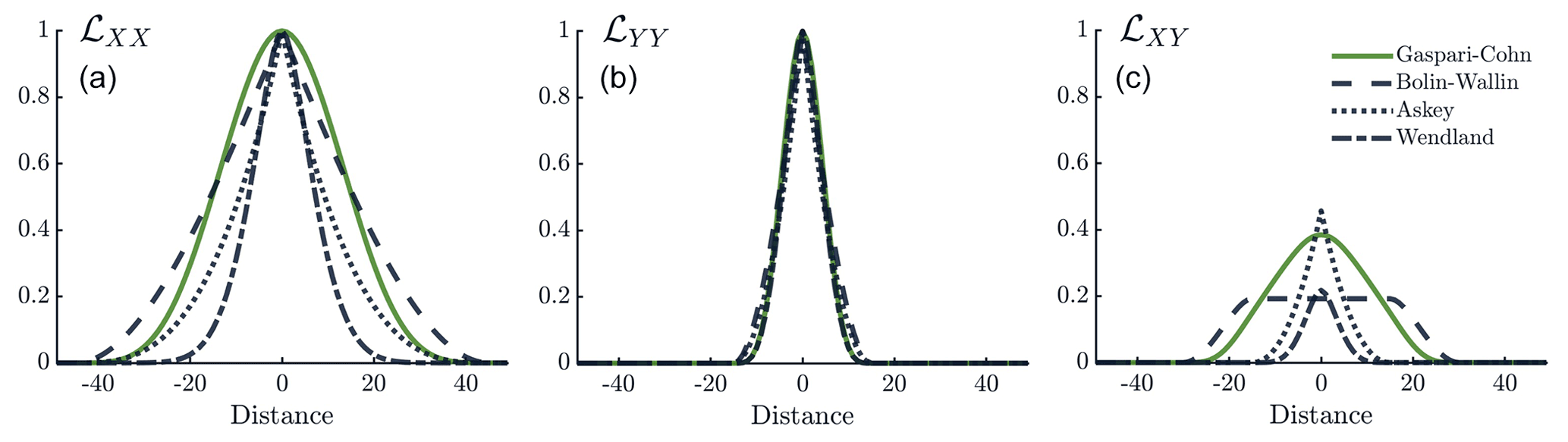
Figure 1There are four multivariate localization functions shown in three panels. Panel (a) shows the function ℒXX used to localize the large process, X. Panel (b) shows the function ℒYY used to localize the small process, Y. Panel (c) shows the cross-localization function ℒXY. In each panel, the color of the line shows the different multivariate functions, i.e., Gaspari–Cohn (green; solid), Bolin–Wallin (dark; dashed), Askey (dark; dotted), and Wendland (dark; dash-dot). In the case of univariate localization, the functions in the middle panel are used to localize all processes. The within-component localization radii are RYY=15 and RXX=45 for all functions. The cross-localization radii are RXY=30 for Gaspari–Cohn and Bolin–Wallin and RXY=15 for Askey and Wendland.
2.4 Multivariate Bolin–Wallin
We derive our second multivariate localization function through convolution of normalized indicator functions over a sphere in ℝ3. As in the previous section, the kernels are supported on spheres of radii cX and cY as follows:
where is an indicator function, which is 1 if r≤cj and 0 otherwise. The resulting within-component localization function with localization radius Rjj=2cj is as follows:
This is commonly referred to as the spherical covariance function. The label BW references Bolin and Wallin, who performed the convolutions necessary to create the associated cross-localization function in a work aimed at a different application of covariance functions (Bolin and Wallin, 2016). While Bolin and Wallin never developed multivariate covariance (or, in our case, localization) functions, the algebra is the same. We present only the localization functions that result from the convolution over ℝ3, though similar functions for ℝ2 and ℝn are available in Bolin and Wallin (2016). Note that there is a typo in Bolin and Wallin (2016), which has been corrected below.
Let cX>cY be kernel radii, and then the resulting cross-localization function is as follows:
Here V3(r,x) denotes the volume of the spherical cap with triangular height x of a sphere with radius r, which is given by the following:
As with multivariate GC, it is convenient to define a ratio of within-component localization radii by . Then we can write the maximum cross-localization weight factor as . The cross-localization radius for BW is because it is created through kernel convolution. An example multivariate BW function with RXX=45, RYY=15, and is shown in Fig. 1.
2.5 Wendland–Gneiting functions
We compare the two functions of the preceding sections to the Wendland–Gneiting family of multivariate, compactly supported, positive semidefinite functions. This family is not generated through kernel convolution but rather through Montée and Descente operators (Gneiting, 2002). The simplest univariate function in this family is the Askey function, which is given by the following:
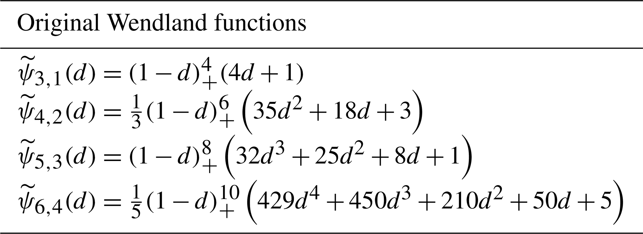
with the shape parameter ν and localization radius R. Other functions in this family are called Wendland functions. Several examples of univariate Wendland functions are displayed in Table 1.
Porcu et al. (2013) developed a multivariate version of the Askey function, where the exponent in Eq. (9) can be different for each process while the localization radius R is constant across all processes. Roh et al. (2015) found that this multivariate localization function outperforms common univariate localization methods when assimilating observations into the bivariate Lorenz 96 model. Daley et al. (2015) extended the work of Porcu et al. (2013) and constructed a multivariate version of general Wendland–Gneiting functions that allow for different localization radii for different processes. The multivariate Askey function from Daley et al. (2015) has the following form:
The general form for multivariate Wendland functions is as follows:
where is defined as follows:
with B as the beta function, . The parameters ν and {γij} are related to the shape of the localization functions and are necessary to guarantee positive semidefiniteness in a given dimension. The parameter k determines the differentiability of the Wendland functions at lag zero (Gneiting, 2002). Note that the Askey function in Eq. (10) is a special case of the Wendland function (Eq. 11), which corresponds to the case k=0. Daley et al. (2015) gave sufficient conditions on the parameters ν, k, Rij, γij, and β to guarantee that Eq. (11) and, hence, Eq. (10) is positive semidefinite. In particular, for the two processes of X and Y, Eq. (11) is positive semidefinite on ℝn when , , , and the following condition holds:
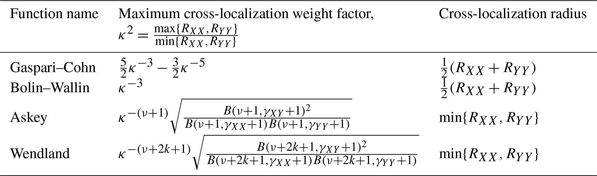
Going forward, we consider the multivariate Askey function (Eq. 10) and the multivariate Wendland function with k=1 in Eq. (11). Note that, with both of these functions, the cross-localization radius depends only on the smallest localization radius. In fact, we choose , although smaller values for RXY also produce positive semidefinite functions. Thus, for given RXX and RYY, the cross-localization radius for Askey and Wendland functions is always smaller than the cross-localization radius for GC and BW. With the choice , we see that βmax depends on the ratio , as in GC and BW. Examples of multivariate Askey and Wendland functions with RXX=45, RYY=15, RXY=15, and are shown in Fig. 1. Important parameters for the four multivariate localization functions presented in this section are summarized in Table 2.
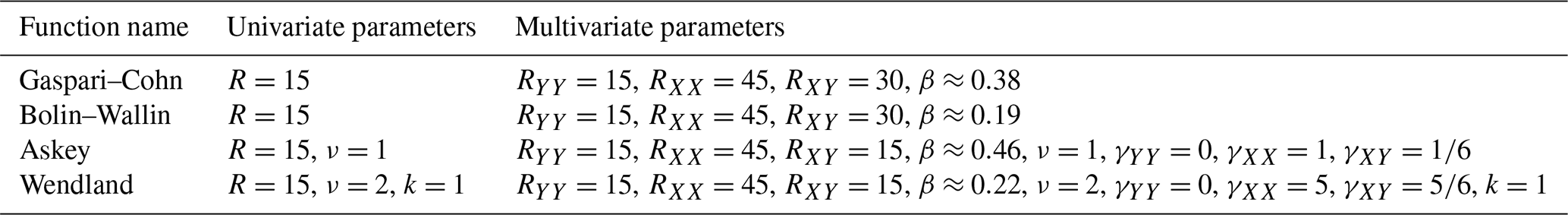
Table 2Summary of important shape parameters for four cross-localization functions.
In this section, we investigate the performance of a data assimilation scheme using each of the four multivariate localization functions presented in Sect. 2. We choose a setup which isolates the impact of the cross-localization functions and relate the filter performance to important cross-localization shape parameters. As a baseline for comparison, we also test two simple approaches to localization for coupled DA. The first method uses a single localization function and radius to localize all within- and cross-component blocks of the background error covariance matrix, i.e., . We call this approach univariate localization. In systems with very different optimal localization radii, this type of univariate localization is likely to perform poorly; however, it does provide a useful comparison point. The second approach uses different localization functions for each process and then zeroes out all cross-correlations between processes, i.e., and ℒXY≡0. We call this approach weakly coupled localization as it leads to a weakly coupled data assimilation scheme. All of the experiments are run with the bivariate Lorenz 96 model, which is described below (Lorenz, 1996).
3.1 Bivariate Lorenz model
The bivariate Lorenz 96 model is a conceptual model of atmospheric processes and is comprised of two coupled processes with distinct temporal and spatial scales. The “small” process can be thought of as rapidly varying small-scale convective fluctuations, while the “large” process can be thought of as smooth large-scale waves. The model is periodic in the spatial domain, as a process on a fixed latitude band would be.
The large process, X, has K distinct variables, Xk for . The small process, Y, is divided into K sectors, with each sector corresponding to one large variable Xk. There are J small process variables in each sector, for a total of JK distinct Y variables, Yj,k for . The Y variables, arranged in order, are . Succinctly, and , with periodicity conditions for all j,k. The X process is also periodic with for all k.
We represent the variables on a circle where the arc length between neighboring Y variables is 1. Equivalently, the radius of the circle is . Variable Yj,k is located at , where . We choose to place the variable Xk, located at (rcos (ϕk),rsin (ϕk)), in the middle of the sector whose variables are coupled to it, e.g., if J=10 then Xk is halfway between Y5,k and Y6,k and . The placement of these variables is illustrated in Fig. 2. The chord distance between any two variables is , where Δθ is the angle increment, e.g., the angle increment between and is .
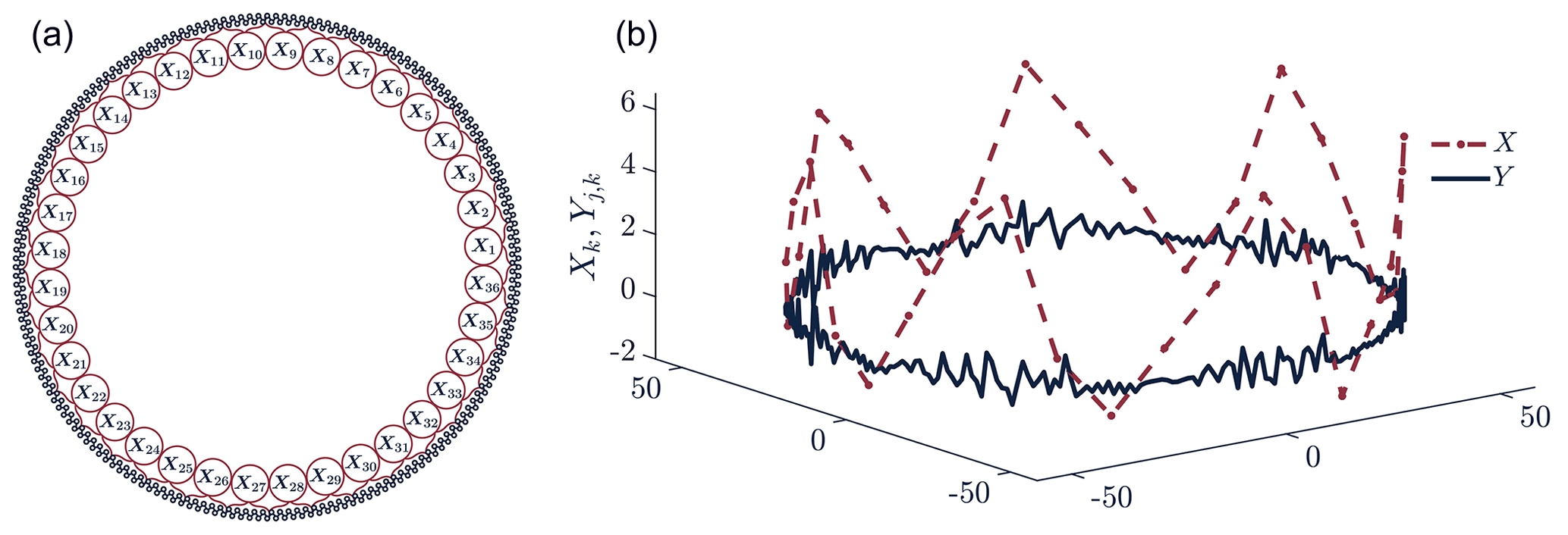
Figure 2(a) Schematic illustrating the location of the different variables in the bivariate Lorenz 96 model, inspired by Wilks (2005). The setup has K=36 sectors, with J=10 small process variables per sector. The large process is shown on the inner circle, and each X variable is labeled. The small process is shown, unlabeled, in the outer circle. Curly brackets show the sectors. (b) A single snapshot of the bivariate Lorenz 96 model with variables placed on a circle. The large process X (red; dashed) has fluctuations with amplitude about 10 times larger than the fluctuation of the small process Y (dark; solid).
The governing equations are as follows:
We follow Lorenz (1996) and let K=36 and J=10, so there are 36 sectors and 10 times more small variables than large variables. We let a=10 and b=10, indicating that convective scales fluctuate 10 times faster than the larger scales, while their amplitude is around one-tenth as large. For the forcing, we choose F=10, which Lorenz (1996) found to be sufficient to make both scales behave chaotically. All simulations are performed using an adaptive fourth-order Runge–Kutta method with relative error tolerance 10−3 and absolute error tolerance 10−6 (Dormand and Prince, 1980; Shampine and Reichelt, 1997). The solutions are output in each assimilation cycle. Unless otherwise specified, the assimilation cycles are separated by a time interval of 0.005 model time units (MTUs), which Lorenz (1996) found to be similar to 36 min in more realistic settings. This timescale is 10 times shorter than the timescale typically used in the univariate Lorenz 96 model. The factor of 10 is consistent with the understanding that the small process evolves 10 times faster than the large process, where the large process is akin to the univariate Lorenz 96 model. In choosing the coupling strength, we follow Roh et al. (2015) and set h=2, which is twice as strong as the coupling used by Lorenz. Varying the coupling strength h across values changes the magnitude of the analysis errors but does not change the relative performance of different localization functions in our experiments.
3.2 Assimilation scheme
In our experiments, we use the stochastic ensemble Kalman filter (EnKF; Evensen, 1994; Houtekamer and Mitchell, 1998; Burgers et al., 1998). The EnKF update formula for a single ensemble member is as follows:
where xa is the analysis vector, xb is the background state vector, y is the observation, each element of η is a random draw from the probability distribution of observation errors, and H is the linear observation operator. The Kalman gain matrix K is as follows:
where Pb is the background error covariance matrix, and R is the observation error covariance matrix. The background covariance matrix is approximated by a sample covariance matrix from an ensemble, i.e., xi for , where Ne is the ensemble size. In this experiment, we use the adaptive inflation scheme of El Gharamti (2018) and inflate each prior ensemble member through the following:
where Λ is a diagonal matrix with each element on the diagonal containing the inflation factor for one variable, and is the background ensemble mean. We then use in place of xb in Eq. (16) and in the estimation of Pb. Note that estimating Pb with the inflated ensemble is equivalent to estimating it with the original ensemble and then multiplying by on the left and right, . The Bayesian approach to adaptive inflation in El Gharamti (2018) uses observations to update the inflation distribution associated with each state variable. The inflation prior has an inverse gamma distribution, with shape and rate parameters determined from the mode and prior inflation variance. In this study, we initialize the inflation factors with Λ=1.1I, where I is the identity matrix. The localization matrix L is incorporated into the estimate of the background covariance matrix through a Schur product, as in Eq. (1).
We use Ne=20 ensemble members, except where otherwise noted. The small ensemble size is chosen to accentuate the spurious correlations and, hence, the need for effective localization functions. We run each DA scheme for 3000 analysis cycles, discarding the first 1000 cycles and reporting statistics from the remaining 2000 cycles. Each experiment is repeated 50 times with independent reference states, which serve as the “truth” in our experiments. We generate “observations” by adding independent Gaussian noise to the reference state.
3.3 Experimental design
The experiments described in this section compare the performance of each of the four multivariate localization functions presented in Sect. 2. Performance is measured through the root mean square (RMS) distance between the analysis mean and the true state, which we refer to as the root mean square error (RMSE). We present scaled analysis errors to aid in comparison between the large and small components. RMS errors are divided by the climatological standard deviation for each process. To standardize the comparison of the different shapes, we use the same within-component localization radii for all multivariate functions. We also investigate the performance of univariate and weakly coupled localization functions. The univariate localization functions are chosen to be equal to the within-component localization function for Y, i.e., ℒ≡ℒYY. The within-component weakly coupled localization functions are equal to the within-component multivariate localization functions. However, the weakly coupled cross-localization functions are identically zero. The free localization function parameters are chosen to balance performance of the univariate, multivariate, and weakly coupled forms of each localization function. We estimate these parameters through a process which we describe in Appendix B.
We test the performance of multivariate localization functions using three different observation operators. First, we observe all small variables and none of the large variables. In this setup, we isolate the impact the of the cross-localization function, which allows us to make conjectures about important cross-localization shape parameters. Next, we flip the setup and observe all large variables and none of the small variables. We compare and contrast our findings with those from the previous case. Finally, we observe both processes and observe behavior reminiscent of both of the previous cases. The experimental setups are grouped by observation operator below. The source code for all experiments is publicly available (see the code availability section).
3.3.1 Observe only the small process
To isolate the impact of the cross-localization functions, we fully observe the small process and do not observe the large process at all. In this configuration, analysis increments of the large process can be fully attributed to the cross-domain assimilation of observations of the small process. The treatment of cross-domain background error covariances plays a crucial role in the analysis of the large process, so we expect that changes in the cross-localization function will lead to changes in the large process analyses. All observations are assimilated every 0.005 MTU. We use an observation error variance of both in the generation of synthetic observations from the reference state and in the assimilation scheme. The observation error variance is chosen to be about 5 % of the climatological variance of the Y process. We also run the experiment with , or about 20 % of the climatological variance, and find that the analyses are degraded, but the relative performance of the different localization functions is the same.
The localization parameters we use in this experiment are given in Table 3. For all functions, we use the maximum allowable cross-localization weight factor, . In estimating the optimal cross-localization weight factor, we find that, since the only updates to X are through observations of Y, smaller cross-localization weight factors lead to degraded performance (Appendix B).
Table 3Localization parameters for the experiment observing only the small process. Note that weakly coupled parameters are not shown in this table because they are exactly equal to the multivariate parameters, except with β=0.
3.3.2 Observe only the large process
Next, we investigate the impact of the different localization functions when we fully observe the large process and do not observe the small process at all. The large process fluctuates about 10 times more slowly than the small process, so we use an assimilation cycle length that is 10 times longer than the one in the previous configuration. All observations are assimilated every 0.05 MTU. We use an observation error variance of both in the generation of synthetic observations from the reference state and in the assimilation scheme. The observation error variance is chosen to be about 5 % of the climatological variance of the X process. We also run the experiment with , or about 20 % of climatological variance, and find that the X analyses are degraded, but the relative performance of the different localization functions is the same. The localization parameters we use in this experiment are given in Table B1. We find that the analysis errors are similar with all values of β. For consistency with the previous experiment, we use the maximum allowable cross-localization weight factor, .
3.3.3 Observe both processes
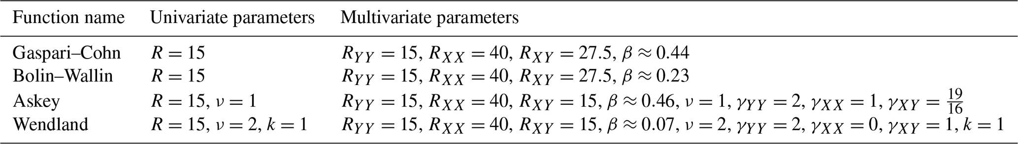
Finally, we observe both processes and note the impact of the different localization functions. In this configuration, we observe 75 % of the variables in each process, with the observation locations chosen randomly for each trial. All observations are assimilated every 0.005 MTU, in line with the analysis cycle length for the observation of the small process only. We use observation error variances of and in the generation of observations and in the assimilation scheme. The observation error variance is chosen to be about 10 % of the climatological variance of each process. We also run the experiment with and , or about 20 % of climatological variance, and find that the performance is similar. The localization parameters we use in this experiment are given in Table B2. We find that the analysis errors grow with increasing β. Nonetheless, to distinguish between multivariate localization, which allows for cross-domain information transfer, and weakly coupled localization, which does not, we use for all multivariate functions.
3.4 Results
3.4.1 Observe only the small process
Figure 3 shows the distribution of analysis errors for the configuration described in Sect. 3.3.1. With weakly coupled localization functions, no information is shared in the update step between the observed Y process and the unobserved X process. This leads to no updates of the X variables and, eventually, to catastrophic filter divergence. In principle, the system might be able to synchronize the unobserved (large) process through dynamical couplings with the observed (small) process, but in our setup, this does not happen. Hence, weakly coupled localization functions are not included in the figure. The analysis error distributions for the observed Y process are similar for all functions except multivariate Wendland. For the unobserved X process, the analysis errors are comparable across all of the univariate localization functions. This is consistent with the fact that all of the univariate localization functions have similar shapes, as seen in Fig. 1b. The multivariate localization functions, on the other hand, show great diversity of performance. The Wendland function leads to significantly worse performance with the multivariate function when compared to the univariate functions. BW and Askey functions perform similarly for both the multivariate and univariate cases. Out of all of the localization functions we consider, the best performance is achieved with multivariate GC.
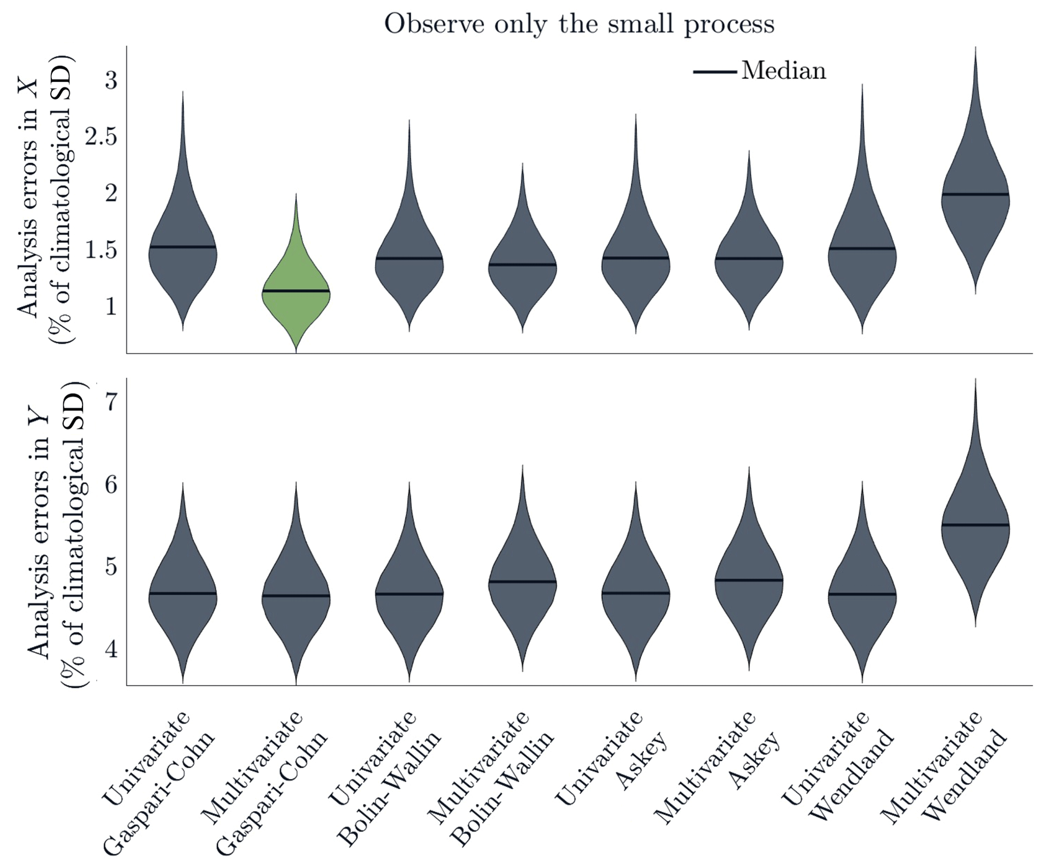
Figure 3Violin plots show the distribution of analysis errors for the X and Y processes with different localization functions (Hoffmann, 2015). Analysis errors are calculated as RMS deviations from the truth and are scaled by the climatological standard deviation of the associated process. All four univariate localization functions perform similarly, while there is a greater range in performance for the multivariate versions of these functions. Multivariate Gaspari–Cohn shows improvement over its univariate counterparts. Univariate and multivariate Bolin–Wallin and Askey functions appear to perform similarly. For Wendland, the multivariate function performs significantly worse than the univariate function.
To understand the improved performance with multivariate GC, we consider two different shape parameters. Recall from Sect. 3.3.1 that smaller cross-localization weights led to worse performance when holding all other localization parameters fixed. Extending this finding, we hypothesize that functions with a larger βmax will allow for more information to propagate across model domains, thereby improving performance in this setup. With the chosen localization parameters, the multivariate Askey function has the largest cross-localization weight factor with , followed by GC with . A visual representation of the cross-localization weight factor is shown as the height of the cross-localization function at zero in Fig. 1c. The shape of each cross-localization function varies not only in its height at zero but also in its radius and smoothness near zero. For example, while the Askey cross-localization function peaks higher than GC, GC is generally smoother near zero and has a larger cross-localization radius. All of these differences in shape impact how much information propagates across model domains. Based on its height and width, we hypothesize that GC allows for sufficient cross-domain information propagation at both small and long distances, and this is why multivariate GC outperforms all other functions in this experiment.
3.4.2 Observe only the large process
When we observe only the large process (as described in Sect. 3.3.2), we find that all localization functions lead to very similar performance. In this case, the shape of the localization function is not important. Rather, the dynamics of the bivariate Lorenz model are driving the behavior. In this configuration, the true background error cross-correlations are very small (less than 0.1 even at small distances). The Y variables are restored towards in their sector (Eq. 15). Thus, even when the assimilation does not update the Y variables, we expect to recover the mean of the Y process. Based on climatology, we find that the conditional mean of Yj,k, given Xk=x, is . The median root mean square difference between Y and its conditional mean is 0.294. Our results show that the median RMSE in the Y process ranges from 0.294 to 0.297. Thus, the filter does not improve upon a simple linear conditional mean prediction, which is perhaps unsurprising given the small magnitude of error cross-correlations. Figure 4 shows the distribution of analysis errors for univariate, weakly coupled, and multivariate GC. The distributions for other functions are nearly identical and, hence, not shown.
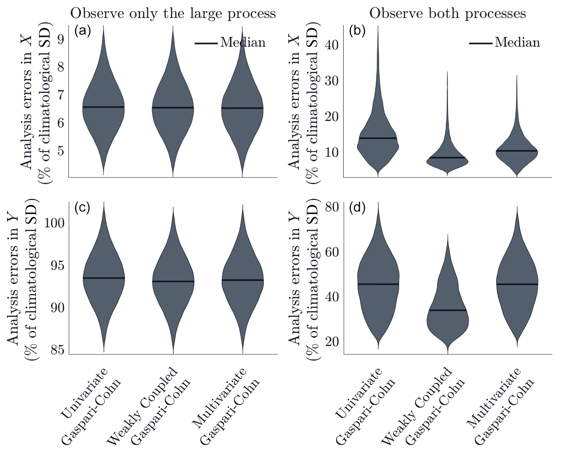
Figure 4Violin plots show the distribution of analysis errors for all versions of the Gaspari–Cohn localization function (Hoffmann, 2015). Analysis errors are calculated as RMS deviations from the truth and are scaled by the climatological standard deviation of the associated process. (a, c) Results from the experiment where we observe only the large process. All functions perform similarly. (b, d) Results from the experiment where we observe both processes. The weakly coupled localization functions appear to lead to the best performance but are highly unstable.
3.4.3 Observe both processes
When we observe both processes, the precise shape of the localization function appears to have little impact. We do see differences between univariate, weakly coupled, and multivariate localization functions. Figure 4 shows analysis error distributions for the three different versions of GC, which are broadly representative of the behavior seen in other functions as well. This configuration is quite unstable. About 80 % of the trials with weakly coupled localization functions lead to catastrophic filter divergence. Trials with univariate and multivariate localization diverge less often, but still diverge about 20 % of the time. Figure 4 shows results from only the trials (out of 50 total) which did not diverge. Weakly coupled localization appears to lead to the best performance, when the filter does not diverge. There is some variation in the results across the different localization functions. In particular, multivariate Askey appears to lead to better performance than weakly coupled Askey, but this may be attributable to the issues with stability. Catastrophic filter divergence is a well-documented but poorly understood phenomenon (Gottwald and Majda, 2013; Houtekamer and Zhang, 2016, their Appendix A). The mechanism is understood in highly idealized models (Kelly et al., 2015), but the dynamics of instability in models as simple as the bivariate Lorenz 96 model remains unclear and is outside the scope of the present investigation.
The complicated story with the weakly coupled schemes indicates that, in this configuration, filter performance is highly sensitive to the treatment of cross-domain background error covariances. The small ensemble size, combined with small true forecast error cross-correlations, can lead to spuriously large estimates of background error cross-covariances. Meanwhile, we have nearly complete observations of both processes, so within-component updates are likely quite good. Thus, zeroing out the cross terms, as in weakly coupled schemes, may improve state estimates. On the other hand, inclusion of some cross-domain terms appears to be important for stability.
In this work, we developed a multivariate extension of the oft-used GC localization function, where the within-component localization functions are standard GC with different localization radii, while the cross-localization function is newly constructed to ensure that the resulting localization matrix is positive semidefinite. A positive semidefinite localization matrix guarantees, through the Schur product theorem, that the localized estimate of the background error covariance matrix is positive semidefinite (Horn and Johnson, 2012, theorem 7.5.3). We compared multivariate GC to three other multivariate localization functions (including one other newly presented multivariate function), and their univariate and weakly coupled counterparts. We found that the performance of different localization functions is highly dependent on the observation operator. When we observed only the large process, all localization functions performed similarly. In an experiment where we observed both processes, weakly coupled localization led to the smallest analysis error. When we observed only the small process, multivariate GC led to better performance than any of the other localization functions we considered. We hypothesized that the shape of the GC cross-localization function allows for larger cross-domain assimilation than the other functions. There is still an outstanding question of how multivariate GC will perform in other, perhaps more realistic, systems.
We found that choosing an appropriate cross-localization weight factor, β, is crucial to the performance of the multivariate localization functions. This parameter determines the amount of information which is allowed to propagate between co-located variables in different model components. We found that this parameter should be as large as possible when observing only the small process. By contrast, the parameter should be small or even zero when both processes are well observed. This is consistent with other studies which have shown the value in deflating cross-domain updates between non-interacting processes (Lu et al., 2015; Yoshida and Kalnay, 2018).
A natural application of this work is localization in a coupled atmosphere–ocean model. The bivariate Lorenz 96 model has a linear relationship between the large and small scales. Hence, the results presented here are relevant to linear coupling in climate models, e.g., the sensible heat exchange between ocean and atmosphere which is approximately linearly proportional to the temperature difference. Multivariate GC allows for within-component covariances to be localized with GC exactly as they would be in an uncoupled setting, using the optimal localization length scale for each component (Ying et al., 2018). The cross-localization length scale for GC is the average of the two within-component localization radii, which is the same as the cross-localization radius proposed in Frolov et al. (2016). We hypothesize that the cross-localization radius is important in determining filter performance. However, the functions considered here did not allow for a thorough investigation of the optimal cross-localization radius, which is an important area for future research.
A1 Multivariate Gaspari–Cohn cross-localization function
Let cX,cY be the kernel radii associated with model components X and Y. Without loss of generality, we take cX>cY. The formula depends on the relative sizes of cX and cY, with two different formulas for the cases (i) cX<2cY and (ii) cX≥2cY. In both cases, the notation is significantly simplified when we let cX=κ2cY. The first case we consider is . In this case, the GC cross-localization function is as follows:
where and . Note that, when we take cX→cY, which implies κ→1, this multivariate function converges to the standard univariate GC function, as we would expect.
The second case to consider is cX>2cY. Again, let cX=κ2cY. In this case, the cross-localization function is as follows:
where, as in the above case, and . Note that when cX=2cY, Eq. (A1) is equal to Eq. (A2).
A2 Derivation of multivariate Gaspari–Cohn cross-localization function
The multivariate GC cross-localization function is created through the convolution of two kernels, , with , , and r∈ℝ3. Theorem 3.c.1 from Gaspari and Cohn (1999) provides a framework for evaluating the necessary convolutions. It is shown that for radially symmetric functions compactly supported on a sphere of radius cj, , with cY≤cX the convolution over ℝ3 given by the following:
can equivalently be written as follows:
Equation (A4) is normalized to produce a localization function with . The normalization factor is given by the following:
The resulting cross-localization function is a normalized version of Eq. (A4), as follows:
With this framework, we are now able to compute the cross-localization function using the GC kernels. We first compute the normalization factor using GC kernels. Plugging in gives the following:
Thus the denominator in Eq. (A6) is as follows:
To compute the numerator in Eq. (A6), which is precisely Eq. (A4), we consider eight different cases, i.e., four cases for each formula presented above.
The case cX>2cY and is shown in detail here. The other cases are derived similarly and are not shown. The inner integral in Eq. (A4) is as follows:
The outer integral in Eq. (A4) is as follows:
which simplifies to the following:
Substituting Eq. (A11) into Eq. (A4) we see the following:
With the proper normalization, we have the cross-localization function as follows:
Now make the substitution , and this then becomes the following:
Other cases are calculated similarly, with careful consideration of the bounds of the kernels and integrals.
A3 Multivariate Gaspari–Cohn with three or more length scales
Suppose we have p processes, with p different localization radii . Define the associate kernel radii by and the associated kernels by . Then the localization function used to taper background error covariances between process Xi and Xj is , with the following:
a positive semidefinite matrix with 1's on the diagonal, i.e., αii=1. When i=j, ℒii is precisely the standard univariate GC function. When i≠j, ℒij is given by Eq. (A1) if or Eq. (A2) otherwise. The ratio of length scales κ is defined as . We have written Eqs. (A1) and (A2) with a coefficient , which is convenient for the case of two components. Here we replace with αij to emphasize the importance for three or more length scales is in choosing αij such that Eq. (A15) is positive semidefinite. Wang et al. (2021) discussed how to construct a similar matrix for multiscale localization using matrix square roots. The simplest case is to let αij=1 for all i,j.
A fair comparison between the univariate, weakly coupled, and multivariate localization functions requires that thoughtful attention be paid to the many parameter choices in the different localization functions. We estimate different localization parameters for each observation operator. This section describes our reasoning behind the selection of the localization parameters for the experiment where we observe only the small process. We follow the same estimation procedure for the other two observation operators as well.
Some of the parameters are shared across functions. For example, every univariate function has a localization radius R. To aid in comparisons between functions, we estimate a single univariate localization radius which is shared by all univariate functions. Indeed, whenever different methods share a parameter we estimate a single value for it. We estimate a separate cross-localization weight factor β for each function because each function has a different upper bound on this parameter.
We estimate the localization parameters iteratively in the following way. First, note that Wendland is a family of functions, with parameter k controlling the smoothness. In sensitivity experiments (not shown), we found that increasing k degrades the performance of the filter. Thus, we choose to use k=1 for all experiments.
Next, we pick appropriate localization radii for each process. We use a large (500-member) ensemble with no localization to compute forecast error correlations (hereafter called the “true” forecast error correlations and shown in Fig. B1). We see that the true forecast error correlations for the small process Y degrade to zero in just a few spatial units. The forecast errors for the large process X, by contrast, have meaningful correlations out to about 40 spatial units. This gives us a baseline for the range of localization radii we should investigate. We compare the performance of all univariate localization functions with the radius . In these sensitivity experiments, we use ν=1 for Askey and ν=2 for Wendland. These values of ν are as small as possible while still guaranteeing positive semidefiniteness. Figure B2 shows that univariate localization radius R=15 leads to the best performance.
Using this univariate localization radius, we now estimate ν for univariate Askey and Wendland. To maintain positive semidefiniteness, we require ν≥1 for Askey and ν≥2 for Wendland. We compare analysis errors for process X and Y with for Askey and for Wendland. In general, we find that smaller values of ν lead to less peaked localization functions and better performance, and we choose ν to be as small as possible, i.e., ν=1 for Askey and ν=2 for Wendland.
Next, we estimate the optimal multivariate localization radii. We want to eliminate as much ambiguity as possible in our comparison of univariate and multivariate localization functions. For this reason, we choose to set the univariate localization radius equal to one of the within-component localization radii. From Fig. B1, we know that the univariate localization radius R=15 is closer to the range of significant true forecast error correlations for process Y than for process X, so we set . Now for the within-X localization radius, we consider the following localization values: . For Askey and Wendland, we use , and γij=0 for all . For all functions we use βmax as the cross-localization weight factor. The analysis errors for both processes are minimized with values of RXX between 40 and 50 (not shown). Informed by the true forecast error correlations, we pick RXX=45. Now we turn to the cross-localization radius. For Gaspari–Cohn and Bolin–Wallin, RXY is determined by RXX and RYY, with . For Askey and Wendland, we require to maintain positive semidefiniteness. From the true forecast error correlations, we see that the correlation length scale for X is larger than the cross-correlation length scale, which is, in turn, larger than the length scale for Y. This intuition tells us that, ideally, we would have . However, because of the requirement for positive semidefiniteness in Askey and Wendland, the closest we can come is . We could choose to use a smaller cross-localization radius, but the true forecast error correlation indicates that this would be a mistake, as there are non-negligible cross-correlations out past 15 units. Thus, we choose .
Using all of the previously estimated multivariate localization parameters, we now estimate γij for all processes for both Askey and Wendland. For Askey, we consider all combinations of and . For Wendland, we consider all combinations of and . The guarantee of positive semidefiniteness restricts our search for γXY to . For simplicity, we take γXY to be at the edge of the allowable range, . While investigating γ, we use the maximum allowable cross-localization weight factor. For Askey, we find that the best performance comes with γXX=1 and γYY=0. For Wendland, we see that performance improves as γXX increases, all the way out to γXX=5. We hypothesize that this is because increasing γXX allows for an increased cross-localization weight factor. We use γXX=5 and γYY=0 for Wendland.
The final localization parameter to estimate is the cross-localization weight factor, β. This parameter determines how much cross-domain information propagation occurs between the X and Y processes. Each multivariate localization function has a different upper bound on β, which depends on a ratio of localization radii, as shown in Fig. B3. Note that setting β=0 leads to a weakly coupled scheme; so, to distinguish between multivariate and weakly coupled, we consider only values of β greater than 0.1. For each multivariate localization function, we vary β between βmax and 0.1, while holding all other parameters fixed. In this setup, the best performance generally comes when the cross-correlation is at or near its maximum allowable value, as shown in Fig. B3. Figure B3 shows visually that the GC cross-correlation is always greater than the BW cross-correlation, which is easily verified analytically since for all κ≥1 (true by the definition of κ). Similarly, we see that the cross-localization weight factor for Askey is greater than cross-localization weight factor for Wendland across the range of parameters considered here.
The localization parameters for the other two observation operators are estimated following the same procedure. The localization parameters for the experiment where we observe only the large process are given in Table B1. The localization parameters for the experiment where we observe both processes are given in Table B2.

Figure B1True forecast error correlations for variables in the middle of each sector, Xk and Y5,k. Correlations between Y variables (dark blue) decay to zero after about 5 spatial units, while correlations between X variables (dark red) are significant up to 40 spatial units away. Cross-correlations (pink and light blue) are small everywhere but still significant out to at least 20 spatial units.
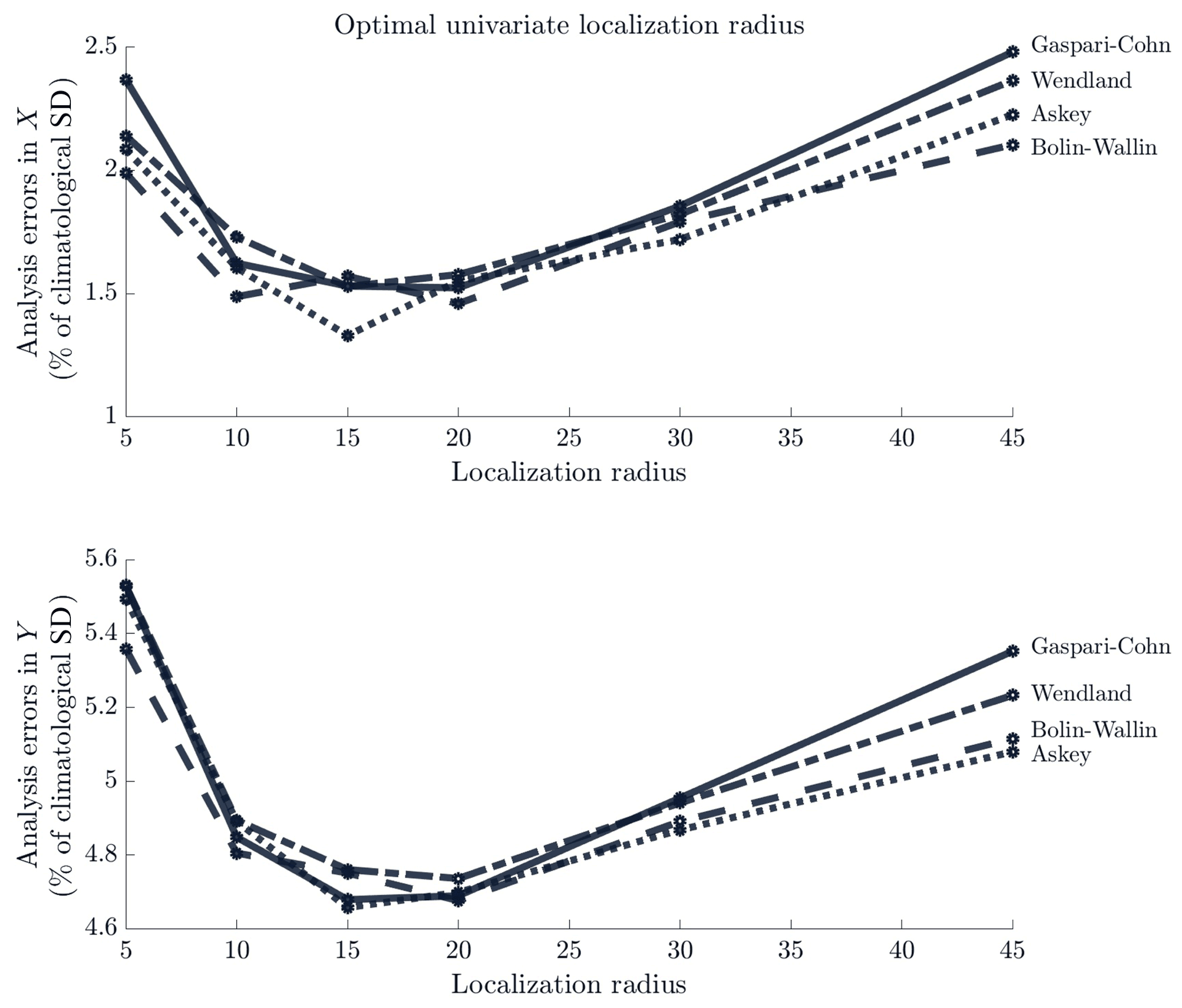
Figure B2Analysis errors for different univariate localization radii. Analysis errors are calculated as RMS deviations from the truth and are scaled by the climatological standard deviation of the associated process. Considering all functions, the best performance comes when R=15.

Figure B3(a) Maximum cross-localization weight factor as a function of . (b, c) Average analysis errors are shown on the y axis for different multivariate functions. The top (bottom) plot shows analysis errors for the X (Y) process. For all functions, as the cross-localization weight factor increases, the analysis errors decrease. Analysis errors are calculated as RMS deviations from the truth and are scaled by the climatological standard deviation of the associated process.
Table B1Localization parameters for the experiment where we observe only the large process.
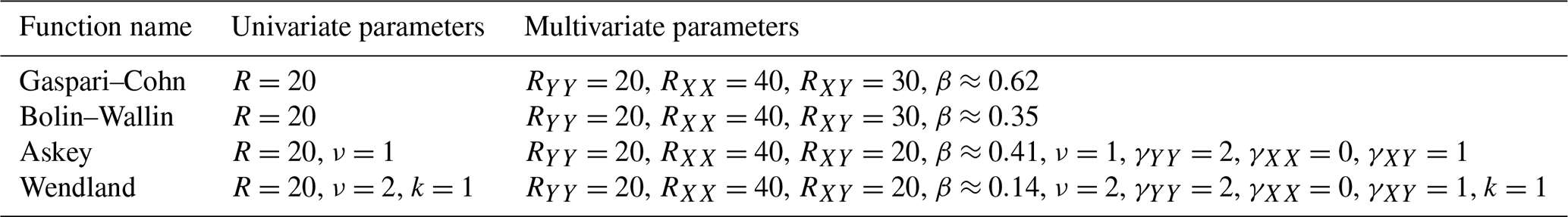
Table B2Localization parameters for the experiment where we observe both processes.
Code used for this study is available in the Zenodo repository at https://doi.org/10.5281/zenodo.4973844 (Stanley, 2021). Data are available in the same repository as the code. All data are generated by the provided code.
The authors all contributed to the conceptualization and formal analysis. ZS and IG contributed to software development. ZS performed the experiments and analysis of the results and prepared the paper, which was edited by IG and WK.
The authors declare they have no conflict of interest.
Publisher’s note: Copernicus Publications remains neutral with regard to jurisdictional claims in published maps and institutional affiliations.
Zofia Stanley has been supported by the National Science Foundation (NSF; grant no. DGE-1650115). Ian Grooms has been supported by the NSF (grant no. DMS-1821074). William Kleiber has been supported by the NSF (grant nos. DMS-1811294 and DMS-1821074). This work utilized resources from the University of Colorado Boulder Research Computing Group, which is supported by the National Science Foundation (grant nos. ACI-1532235 and ACI-1532236), the University of Colorado Boulder, and Colorado State University. The authors thank Olivier Talagrand, for handling the review of this paper, and Stephen G. Penny and two other anonymous reviewers, for their input.
This research has been supported by the National Science Foundation (grant nos. DGE-1650115, DMS-1821074, and DMS-1811294).
This paper was edited by Olivier Talagrand and reviewed by Stephen G. Penny and two anonymous referees.
Anderson, J. L.: Localization and sampling error correction in ensemble Kalman filter data assimilation, Mon. Weather Rev., 140, 2359–2371, 2012. a
Bannister, R. N.: A review of forecast error covariance statistics in atmospheric variational data assimilation. I: Characteristics and measurements of forecast error covariances, Q. J. Roy. Meteor. Soc., 134, 1951–1970, https://doi.org/10.1002/qj.339, 2008. a
Bishop, C. H. and Hodyss, D.: Flow-adaptive moderation of spurious ensemble correlations and its use in ensemble-based data assimilation, Q. J. Roy. Meteor. Soc., 133, 2029–2044, 2007. a
Bolin, D. and Wallin, J.: Spatially adaptive covariance tapering, Spat. Stat., 18, 163–178, https://doi.org/10.1016/j.spasta.2016.03.003, 2016. a, b, c, d
Buehner, M. and Shlyaeva, A.: Scale-dependent background-error covariance localisation, Tellus A, 67, 28027, https://doi.org/10.3402/tellusa.v67.28027, 2015. a
Burgers, G., van Leeuwen, P. J., and Evensen, G.: Analysis Scheme in the Ensemble Kalman Filter, Mon. Weather Rev., 126, 1719–1724, https://doi.org/10.1175/1520-0493(1998)126<1719:ASITEK>2.0.CO;2, 1998. a
Daley, D. J., Porcu, E., and Bevilacqua, M.: Classes of compactly supported covariance functions for multivariate random fields, Stoch. Env. Res. Risk A., 29, 1249–1263, https://doi.org/10.1007/s00477-014-0996-y, 2015. a, b, c, d
Dormand, J. and Prince, P.: A family of embedded Runge-Kutta formulae, J. Comput. Appl. Math., 6, 19–26, https://doi.org/10.1016/0771-050X(80)90013-3, 1980. a
El Gharamti, M.: Enhanced Adaptive Inflation Algorithm for Ensemble Filters, Mon. Weather Rev., 146, 623–640, https://doi.org/10.1175/MWR-D-17-0187.1, 2018. a, b
Evensen, G.: Sequential data assimilation with a nonlinear quasi-geostrophic model using Monte Carlo methods to forecast error statistics, J. Geophys. Res.-Oceans, 99, 10143–10162, https://doi.org/10.1029/94JC00572, 1994. a
Frolov, S., Bishop, C. H., Holt, T., Cummings, J., and Kuhl, D.: Facilitating Strongly Coupled Ocean–Atmosphere Data Assimilation with an Interface Solver, Mon. Weather Rev., 144, 3–20, https://doi.org/10.1175/MWR-D-15-0041.1, 2016. a, b, c, d
Frolov, S., Reynolds, C. A., Alexander, M., Flatau, M., Barton, N. P., Hogan, P., and Rowley, C.: Coupled Ocean–Atmosphere Covariances in Global Ensemble Simulations: Impact of an Eddy-Resolving Ocean, Mon. Weather Rev., 149, 1193–1209, https://doi.org/10.1175/MWR-D-20-0352.1, 2021. a, b
Gaspari, G. and Cohn, S. E.: Construction of correlation functions in two and three dimensions, Q. J. Roy. Meteor. Soc., 125, 723–757, https://doi.org/10.1002/qj.49712555417, 1999. a, b, c, d
Genton, M. G. and Kleiber, W.: Cross-Covariance Functions for Multivariate Geostatistics, Stat. Sci., 30, 147–163, https://doi.org/10.1214/14-STS487, 2015. a, b, c
Gneiting, T.: Compactly Supported Correlation Functions, J. Multivariate Anal., 83, 493–508, https://doi.org/10.1006/jmva.2001.2056, 2002. a, b
Gottwald, G. A. and Majda, A. J.: A mechanism for catastrophic filter divergence in data assimilation for sparse observation networks, Nonlin. Processes Geophys., 20, 705–712, https://doi.org/10.5194/npg-20-705-2013, 2013. a
Greybush, S. J., Kalnay, E., Miyoshi, T., Ide, K., and Hunt, B. R.: Balance and Ensemble Kalman Filter Localization Techniques, Mon. Weather Rev., 139, 511–522, https://doi.org/10.1175/2010MWR3328.1, 2011. a
Hoffmann, H.: Violin Plot, available at: https://www.mathworks.com/matlabcentral/fileexchange/45134-violin-plot (last access: June 2021), 2015. a, b
Horn, R. A. and Johnson, C. R.: Matrix analysis, 2nd edn., Cambridge University Press, Cambridge, New York, 2012. a, b
Houtekamer, P. L. and Mitchell, H. L.: Data Assimilation Using an Ensemble Kalman Filter Technique, Mon. Weather Rev., 126, 796–811, https://doi.org/10.1175/1520-0493(1998)126<0796:DAUAEK>2.0.CO;2, 1998. a
Houtekamer, P. L. and Mitchell, H. L.: A Sequential Ensemble Kalman Filter for Atmospheric Data Assimilation, Mon. Weather Rev., 129, 123–137, https://doi.org/10.1175/1520-0493(2001)129<0123:ASEKFF>2.0.CO;2, 2001. a
Houtekamer, P. L. and Zhang, F.: Review of the Ensemble Kalman Filter for Atmospheric Data Assimilation, Mon. Weather Rev., 144, 4489–4532, https://doi.org/10.1175/MWR-D-15-0440.1, 2016. a
Kelly, D., Majda, A. J., and Tong, X. T.: Concrete ensemble Kalman filters with rigorous catastrophic filter divergence, P. Natl. Acad. Sci. USA, 112, 10589–10594, https://doi.org/10.1073/pnas.1511063112, 2015. a
Lorenz, E. N.: Predictability – A problem partly solved, vol. 1, pp. 1–18, Proc. Seminar on Predictability, ECMWF, Reading, Berkshire, United Kingdom, 1996. a, b, c, d, e
Lu, F., Liu, Z., Zhang, S., and Liu, Y.: Strongly Coupled Data Assimilation Using Leading Averaged Coupled Covariance (LACC). Part I: Simple Model Study, Mon. Weather Rev., 143, 3823–3837, https://doi.org/10.1175/MWR-D-14-00322.1, 2015. a, b, c, d
Morss, R. E. and Emanuel, K. A.: Influence of added observations on analysis and forecast errors: Results from idealized systems, Q. J. Roy. Meteor. Soc., 128, 285–321, https://doi.org/10.1256/00359000260498897, 2002. a
Ménétrier, B., Montmerle, T., Michel, Y., and Berre, L.: Linear Filtering of Sample Covariances for Ensemble-Based Data Assimilation. Part I: Optimality Criteria and Application to Variance Filtering and Covariance Localization, Mon. Weather Rev., 143, 1622–1643, https://doi.org/10.1175/MWR-D-14-00157.1, 2015. a
Penny, S. G., Bach, E., Bhargava, K., Chang, C.-C., Da, C., Sun, L., and Yoshida, T.: Strongly Coupled Data Assimilation in Multiscale Media: Experiments Using a Quasi-Geostrophic Coupled Model, J. Adv. Model. Earth Sy., 11, 1803–1829, https://doi.org/10.1029/2019MS001652, 2019. a
Porcu, E., Daley, D. J., Buhmann, M., and Bevilacqua, M.: Radial basis functions with compact support for multivariate geostatistics, Stoch. Env. Res. Risk A., 27, 909–922, https://doi.org/10.1007/s00477-012-0656-z, 2013. a, b
Roh, S., Jun, M., Szunyogh, I., and Genton, M. G.: Multivariate localization methods for ensemble Kalman filtering, Nonlin. Processes Geophys., 22, 723–735, https://doi.org/10.5194/npg-22-723-2015, 2015. a, b, c, d
Shampine, L. F. and Reichelt, M. W.: The MATLAB ODE Suite, SIAM J. Sci. Comput., 18, 1–22, https://doi.org/10.1137/S1064827594276424, 1997. a
Shen, Z., Tang, Y., Li, X., Gao, Y., and Li, J.: On the localization in strongly coupled ensemble data assimilation using a two-scale Lorenz model, Nonlin. Processes Geophys. Discuss. [preprint], https://doi.org/10.5194/npg-2018-50, 2018. a
Sluka, T. C., Penny, S. G., Kalnay, E., and Miyoshi, T.: Assimilating atmospheric observations into the ocean using strongly coupled ensemble data assimilation, Geophys. Res. Lett., 43, 752–759, https://doi.org/10.1002/2015GL067238, 2016. a
Smith, P. J., Lawless, A. S., and Nichols, N. K.: Estimating Forecast Error Covariances for Strongly Coupled Atmosphere–Ocean 4D-Var Data Assimilation, Mon. Weather Rev., 145, 4011–4035, https://doi.org/10.1175/MWR-D-16-0284.1, 2017. a, b
Smith, P. J., Lawless, A. S., and Nichols, N. K.: Treating Sample Covariances for Use in Strongly Coupled Atmosphere-Ocean Data Assimilation, Geophys. Res. Lett., 45, 445–454, https://doi.org/10.1002/2017GL075534, 2018. a, b, c
Smith, P. J., Lawless, A. S., and Nichols, N. K.: The role of cross-domain error correlations in strongly coupled 4D-Var atmosphere–ocean data assimilation, Q. J. Roy. Meteor. Soc., 146, 2450–2465, https://doi.org/10.1002/qj.3802, 2020. a
Stanley, Z.: zcstanley/Multivariate_Localization_Functions: Code for resubmission (2.0), Zenodo [code], https://doi.org/10.5281/zenodo.4973844, 2021. a
Wang, X., Chipilski, H. G., Bishop, C. H., Satterfield, E., Baker, N., and Whitaker, J. S.: A Multiscale Local Gain Form Ensemble Transform Kalman Filter (MLGETKF), Mon. Weather Rev., 149, 605–622, https://doi.org/10.1175/MWR-D-20-0290.1, 2021. a
Wilks, D. S.: Effects of stochastic parametrizations in the Lorenz '96 system, Q. J. Roy. Meteor. Soc., 131, 389–407, https://doi.org/10.1256/qj.04.03, 2005. a
Ying, Y., Zhang, F., and Anderson, J. L.: On the Selection of Localization Radius in Ensemble Filtering for Multiscale Quasigeostrophic Dynamics, Mon. Weather Rev., 146, 543–560, https://doi.org/10.1175/MWR-D-17-0336.1, 2018. a, b
Yoshida, T. and Kalnay, E.: Correlation-Cutoff Method for Covariance Localization in Strongly Coupled Data Assimilation, Mon. Weather Rev., 146, 2881–2889, https://doi.org/10.1175/MWR-D-17-0365.1, 2018. a, b, c
- Abstract
- Introduction
- Multivariate localization functions
- Experiments
- Conclusions
- Appendix A: Derivation of multivariate Gaspari–Cohn
- Appendix B: Estimation of localization parameters
- Code and data availability
- Author contributions
- Competing interests
- Disclaimer
- Acknowledgements
- Financial support
- Review statement
- References