the Creative Commons Attribution 4.0 License.
the Creative Commons Attribution 4.0 License.
 | 17 Sep 2020
Review article: Hilbert problems for the climate sciences in the 21st century – 20 years later
The scientific problems posed by the Earth's atmosphere, oceans, cryosphere – along with the land surface and biota that interact with them – are central to major socioeconomic and political concerns in the 21st century. It is natural, therefore, that a certain impatience should prevail in attempting to solve these problems. The point of a review paper published in this journal in 2001 was that one should proceed with all diligence but not excessive haste, namely “festina lente”, i.e., “to hurry in a measured way”. The earlier paper traced the necessary progress through the solutions of 10 problems, starting with “What can we predict beyond 1 week, for how long, and by what methods?” and ending with “Can we achieve enlightened climate control of our planet by the end of the century?”
A unified framework was proposed to deal with these problems in succession, from the shortest to the longest timescale, i.e., from weeks to centuries and millennia. The framework is that of dynamical systems theory, with an emphasis on successive bifurcations and the ergodic theory of nonlinear systems, on the one hand, and on pursuing this approach across a hierarchy of climate models, from the simplest, highly idealized ones to the most detailed ones. Here, we revisit some of these problems, 20 years later,1 and extend the framework to coupled climate–economy modeling.


In order to assess to what extent and in which ways we are modifying our global environment, it is essential to understand how this environment functions. In the past 2 decades, it has become abundantly clear that we do affect the climate system, both globally and locally (IPCC, 1990, 2001, 2007, 2014a), but many of the uncertainties and missing details are still with us.
We take herein, therefore, a planetary view of the Earth's climate system, of the pieces it contains, and of the way these pieces interact. This will allow us to eventually understand, predict with confidence and with known error margins and, ultimately, exert some rational control on the individual pieces and, thus, on the whole of such a complex system.
Some readers of the earlier paper will notice a slight change in the title. The climate sciences used in the title now have evolved rather rapidly over the last 2 decades and have become a fairly broad field in their own right. Rather than casting an even wider net to encompass all of the geosciences, we decided to claim merely the climate sciences as the topic. On the other hand, the problem of mitigating the effects of climate change and adapting to them cannot be solved without a thorough understanding of basic economic principles. The need for such an understanding, and for weaving it into the solution of the last problem, has led to the need for casting a wider net in the direction of macroeconomic data analysis and modeling.
Several research groups carried out an important extension of the dynamical systems and model hierarchy framework of Ghil (2001) during the past 2 decades, from deterministically autonomous to nonautononomous and random dynamical systems (NDS and RDS; e.g., Ghil et al., 2008; Chekroun et al., 2011; Bódai and Tél, 2012). This framework allows one to deal, in a self-consistent way, with the increasing role of time-dependent forcing applied to the Earth system by humanity and by natural processes, such as solar variability and volcanic eruptions. Ghil (2019, Sect. 5.3) and Ghil and Lucarini (2019, Sect. IV.E) recently provided a fairly complete review of these advances, and we shall thus mention them herein only in passing.
The 10 problems proposed in Ghil (2001) to achieve this goal were:
-
What is the coarse-grained structure of low-frequency atmospheric variability, and what is the connection between its episodic and oscillatory description?
-
What can we predict beyond 1 week, for how long, and by what methods?
-
What are the respective roles of intrinsic ocean variability, coupled ocean–atmosphere modes, and atmospheric forcing in seasonal to interannual variability?
-
What are the implications of the answer to the previous problem for climate prediction on this timescale?
-
How does the oceans' thermohaline circulation change on interdecadal and longer timescales, and what is the role of the atmosphere and sea ice in such changes?
-
What is the role of chemical cycles and biological changes in affecting climate on slow timescales, and how are they affected, in turn, by climate variations?
-
Does the answer to the question above give us some trigger points for climate control?
-
What can we learn about these problems from the atmospheres and oceans of other planets and their satellites?
-
Given the answers to the questions so far, what is the role of humans in modifying the climate?
-
Can we achieve enlightened climate control of our planet by the end of the century?
These problems were listed in increasing order of timescale, from the shortest to the longest one, i.e., from weeks to centuries and millennia. Ghil (2001) emphasized the fact that, in mathematics, clearly formulated problems can be given fully satisfactory solutions. Thus, in his “Lecture delivered before the International Congress of Mathematicians at Paris in 1900,” David Hilbert2 proposed 10 problems, whose number was increased to 23 in a subsequent publication (Hilbert, 1900). In fact, of the properly formulated Hilbert problems, 10 problems, namely , have a resolution that is accepted by a general consensus of the mathematical community. On the other hand, the solutions proposed for seven problems, namely , are only partially accepted as resolving the corresponding problems.
That leaves problems 8 (the Riemann hypothesis), 12, and 16 unresolved, while 4 and 23 were too vaguely formulated to ever be described as solved. Problem 6 is of particular interest to us here. Its overall heading (Hilbert, 1900) is the “Mathematical treatment of the axioms of physics,” meaning that one should treat them in the same way as the “foundations of geometry”. This problem has been interpreted as having the following two subproblems: (a) an axiomatic treatment of probability that will yield limit theorems for the foundation of statistical physics, and (b) a rigorous theory of limiting processes “which lead from the atomistic view to the laws of motion of continua,” e.g., from Boltzmann's equations of statistical mechanics to the partial differential equations of continuous media. The mathematical community considers that the axiomatic formulation of the probability theory by Kolmogoroff (2019) is an entirely satisfactory solution to part (a), although alternative formulations do exist; part (b) is work in progress.
On the contrary, problems in the physical sciences – let alone in the life sciences or socioeconomic sciences – cannot be “solved”, in general, to everybody's satisfaction in finite time. Apparently, though, social media do entertain the notion of “Hilbert problems for social justice warriors,” whatever that may mean.
The 10 original problems of Ghil (2001) could easily be complemented with 13 more, and the unanswered problems of the climate sciences would still be far from exhausted. We illustrate, instead, in the rest of this paper how attempts to solve four of the 10 problems above – namely problems 1, 2, 3, and 10 – have fared over the intervening 2 decades and do so quite succinctly. Sections 2 and 3 deal with problems 1 and 2 and with problem 3, respectively. Sections 4 and 5, in turn, address two complementary aspects of problem 10, namely the climate and coupling part versus the economic part. Concluding remarks follow in Sect. 6, and Appendix A provides some technical details on the results concerning fluctuation–dissipation in macroeconomics.
In the climate sciences, like in all the sciences, terms like “low frequency” and “long term” have to be defined quantitatively. The dominant frequency band in midlatitude day-to-day weather is the so-called synoptic frequency of the evolution of extratropical weather systems, which corresponds to periodicities of 5–10 d. Thus, for the atmosphere, low-frequency variability (LFV) and medium-range forecasting refer to time intervals longer than 10 d.
As recently mentioned in Ghil et al. (2018) and Ghil and Lucarini (2019), it was John von Neumann (1903–1957), at the very beginnings of climate dynamics, who made an important distinction (Von Neumann, 1960) between weather and climate prediction. To wit, short-term numerical weather prediction (NWP) is the easiest form of prediction, i.e., it is a pure initial-value problem; long-term climate prediction is the next easiest as it corresponds to studying the system's asymptotic behavior; intermediate-term prediction is hardest – both initial and boundary values are important. In this case, the boundary values refer mainly to the boundary conditions at the air–sea and air–land interfaces.
Essentially, the first of the three problems above corresponds to Lorenz's predictability of the first kind, while the second one corresponds to his predictability of the second kind (Lorenz, 1967; Peixoto and Oort, 1992). It is the intermediate-term prediction that requires going beyond the initial-value problem but without reaching all the way to a statistical equilibrium for very long times. It is this problem that requires a unified treatment of slower climate change in the presence of faster climate variability, and we return to it in Sects. 3 and 4.
Concerning the study of atmospheric LFV and medium-range forecasting, Ghil (2001) had little to say about them at the time. Both areas of inquiry, though, have taken huge strides over the last 2 or 3 decades (e.g., Kalnay, 2003; Palmer, 2017); the weather forecast for planning one's holiday at the beach or in the mountains next week has become considerably more reliable. Still, a key issue associated with problem 1 was formulated by Ghil and Robertson (2002), namely whether it is the “wave” point of view or the “particle” one that is more helpful in observing, describing, and predicting LFV. To wit, is it (i) oscillatory modes with periods of 30 d and longer, namely the waves, or (ii) persistent anomalies with durations of 10 d or longer and the Markov chains of transitions between more or less persistent regimes, namely the particles, that are more interesting and useful in coming to grips with medium-range forecasting?
Ghil et al. (2018) have reformulated this problem more completely in Fig. 1. Here, diagram (a) represents Markov chains between two or more flow regimes with distinct spatial patterns and stability properties, such as blocked (B) and zonal (Z; Charney and DeVore, 1979, and references therein) or Pacific–North-American (PNA), Reverse PNA (RNA), and the blocked phase of the North Atlantic Oscillation (BNAO; Kimoto and Ghil, 1993a; Smyth et al., 1999).
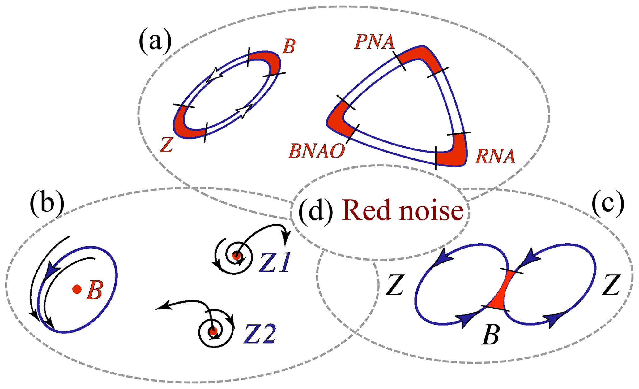
Figure 1Schematic overview of atmospheric low-frequency variability (LFV) mechanisms. Reprinted from Ghil et al. (2018), with permission from Elsevier.
Diagram (b) in Fig. 1 is associated with the idea of oscillatory instabilities of one or more of the multiple fixed points that can play the role of regime centroids. Thus, Legras and Ghil (1985) found a 40 d oscillation due to a Hopf bifurcation off their blocked regime, B, while Z1 and Z2 in their model were generalized saddles that both had zonal flow patterns. An ambiguity arises, though, between this point of view and a complementary possibility, namely that the regimes are just slow phases of such an oscillation, caused itself by the interaction of the midlatitude jet with topography. Thus, Kimoto and Ghil (1993b) found, in their observational data, closed paths within a Markov chain in which the states resemble well-known phases of an intraseasonal oscillation. Furthermore, multiple regimes and intraseasonal oscillations can coexist in a two-layer model on the sphere within the scenario of “chaotic itinerancy” (Itoh and Kimoto, 1997).
Diagram (c) in Fig. 1 is a sketch of the linear point of view that persistent anomalies in midlatitude atmospheric flows on 10–100 d timescales are just due to the slowing down of Rossby waves or to their linear interference (Lindzen, 1986). An interesting extension of this approach into the nonlinear realm is due to Nakamura and associates (Nakamura and Huang, 2018; Paradise et al., 2019). The traffic jam analogy for blocking in this work is somewhat similar to the hydraulic jump analogy of Rossby and collaborators (1939); see also Malone et al. (1951/1955/2016, p. 432).
Finally, diagram (d) of Fig. 1 corresponds to the effects of stochastic perturbations on any of the (a)–(c) scenarios (Hasselmann, 1976; Kondrashov et al., 2006; Palmer and Williams, 2009).
Recently, Lucarini and Gritsun (2020) made an interesting step in reconciling scenarios (a) and (b) in the figure. These authors used a fairly realistic, three-level quasi-geostrophic (QG3) model (Marshall and Molteni, 1993; Kondrashov et al., 2006) to study blocking events through the lens of unstable periodic orbits (UPOs; Cvitanović and Eckhardt, 1989; Gilmore, 1998). UPOs are natural modes of variability that densely populate a chaotic system's attractor. Lucarini and Gritsun (2020) found that blockings occur when the system's trajectory is in the neighborhood of a specific class of UPOs.
The UPOs that correspond to blockings in the QG3 model are more unstable than the UPOs associated with zonal flow; thus, blockings are associated with anomalously unstable atmospheric states, as suggested theoretically by Legras and Ghil (1985) and confirmed experimentally in a rotating annulus with bottom topography by Weeks et al. (1997); see also Ghil and Childress (1987/2012, chap. 6). Different regimes (particles) may be associated with different bundles of UPOs (waves).
Given this perspective on atmospheric LFV, what can be said about the predictability of flow features in the 10–100 d window between the limit of detailed, deterministic predictability, on the one hand (e.g., Lorenz, 1969), and the large changes induced in the atmospheric circulation by the march of seasons, on the other? Clearly, the occurrence of certain flow patterns that are more frequently observed, and thus associated with clusters or regimes, should be more predictable. The relative success of Markov chains in describing the transitions between qualitatively different regimes is consistent with the results of Lucarini and Gritsun (2020).
Ghil et al. (2018) have carried out a detailed review of many studies on what used to be called intraseasonal atmospheric variability and is more recently being called subseasonal to seasonal (S2S) variability. They concluded that the number and variety of methods that have been used to identify and describe LFV regimes are leading up to a tentative consensus on their existence, robustness, and characteristics. S2S forecasting has become operationally viable and is under intensive investigation (e.g., Robertson and Vitart, 2018, and references therein).
A remarkable feature of human nature is the tendency to always put the blame elsewhere – rather than at one's own doorstep. Thus, meteorologists tended to blame sea surface temperatures (SSTs) for changes in atmospheric circulation on S2S timescales and longer, while oceanographers blamed changes in the wind stress for such changes in the upper ocean. It is more judicious, though, to ask “What are the respective roles of intrinsic ocean variability, coupled ocean–atmosphere modes, and atmospheric forcing in seasonal to interannual variability?” as done in problem 3 of Ghil (2001).
The difference between the two approaches is largely one between linear thinking, in which changes in a system at frequencies not present in its free modes have to be due to external agencies, and nonlinear thinking, in which combination tones and other more complex spectral features may be present. Moreover, interactions between subsystems and between any subsystem and time-dependent forcing can be much richer in a nonlinear world. We will briefly sketch the evolution of the latter point of view in the study of oceanic interannual variability here.
A paradigmatic example of how complex intrinsic LFV can arise in the ocean circulation is the so-called double-gyre problem (e.g., Ghil et al., 2008; Ghil, 2017). Note that the synoptic timescale in the oceans is associated with the oceanic counterpart of “weather” – i.e., with the lifetime of so-called mesoscale eddies – and it is of months rather than a week or two (Gill, 1982; Pedlosky, 1996). Hence, LFV in the ocean corresponds to several years rather than to 1–3 months.
Veronis (1963) already obtained the bistability of steady solutions in a single-gyre configuration and a stable limit cycle for time-independent wind stress. Jiang et al. (1995) studied the successive bifurcation tree all the way to chaotic solutions in a double-gyre model with steady time-independent forcing. The periodic solutions they obtained were pluriannual, had the characteristics of relaxation oscillations, and were termed gyre modes because of the strong vortices they exhibited on either side of the separation of the model's eastward jet from the western boundary (Dijkstra and Ghil, 2005).
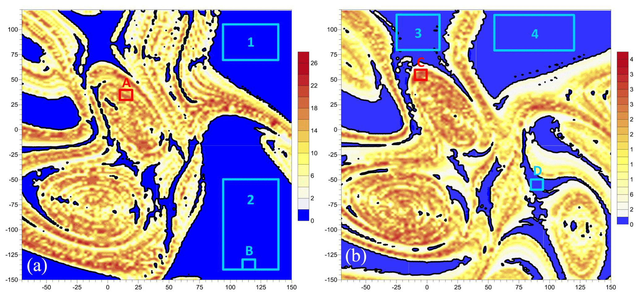
Figure 2Numerical evidence for the existence of two local pullback attractors (PBAs) in the wind-driven midlatitude ocean circulation. Plotted is a mean normalized distance, Δ, for 15 000 trajectories of the double-gyre ocean model of Pierini et al. (2016, 2018); the cold colors correspond to very quiescent behavior, while the warm colors are associated with unstable, chaotic motion on the PBA. The parameter values in the two panels are, respectively, subcritical and supercritical in the autonomous version of the model with respect to the homoclinic bifurcation that gives rise to relaxation oscillations in the latter – (a) γ=0.96 and (b) γ=1.1. Reproduced from Pierini et al. (2016). © American Meteorological Society; used with permission.
Pierini et al. (2016, 2018) applied, to simplified double-gyre models, the previously mentioned NDS theory. These authors found that, even in the presence of time-dependent forcing and of a unique global pullback attractor (PBA), two local PBAs with very different stability properties can coexist, and their mutual boundary appears to be fractal; see Fig. 2 here and the more detailed explanations in Ghil (2019, Fig. 12). Ghil (2017) and Ghil and Lucarini (2019) reviewed both the fundamental ideas of NDS and RDS theory and their applications to climate problems; hence, little more will be said herein on these topics.
Feliks et al. (2004, 2007) showed that a narrow and sufficiently strong SST front with the 7 year periodicity of the oceanic gyre modes could give rise to a similar near periodicity in the atmospheric jet stream above the oceanic eastward jet, provided the resolution of the atmospheric model was sufficiently high; see also Minobe et al. (2008). Groth et al. (2017) studied reanalysis fields for both ocean and atmosphere over the North Atlantic basin and adjacent land areas (25–65∘ N, 80–0∘ W); they found their results to be in good agreement with the dominant 7–8 year periodicity of the North Atlantic Oscillation (NAO) being due to the intrinsic periodicity of barotropic gyre modes. The agreement with the alternative theory of a turbulent oscillator (Berloff et al., 2007) playing a key role in the NAO was less evident since the latter depends, in an essential way, on strong baroclinic activity and has a much broader spectral peak that does not emphasize the NAO's 7–8 year peak.
On the other hand, Vannitsem et al. (2015) investigated oceanic LFV in a coupled ocean–atmosphere model with a total of 36 Fourier modes. Their results included stable decadal-scale periodic orbits with a strong atmospheric component, and chaotic solutions that were still dominated by the decadal behavior. Projecting atmospheric and oceanic reanalysis data sets onto the leading modes of the Vannitsem et al. (2015) model, Vannitsem and Ghil (2017) confirmed that a dominant LFV signal with a 25–30 year period (Timmermann et al., 1998; Frankcombe and Dijkstra, 2011) is a common mode of variability of the atmosphere and oceans.
Clearly, the separation between the wind-driven circulation addressed by problem 3 and the buoyancy-driven circulation addressed by problem 5 is rather a matter of convenience as a water particle in the ocean is affected by both types of forces. Moreover, recently, Cessi (2019, and references therein) have argued that the meridional overturning is actually powered by momentum fluxes and not by buoyancy fluxes. This argument is not quite generally accepted; see, for instance, Tailleux (2010). Given the lack of consensus about the matter, the thermohaline circulation of problem 5 is increasingly termed the oceans' meridional overturning circulation, thus avoiding a definite attribution of its physical causes.
In the studies of atmospheric, oceanic, and coupled variability of the climate system, considerable progress has been made in applying dynamical systems theory and, in particular, bifurcation theory to models subject to time-dependent forcing (Alkhayuon et al., 2019) or to models that lie further towards the high end (Rahmstorf et al., 2005; Hawkins et al., 2011) of the model hierarchy originally proposed by Schneider and Dickinson (1974). More recently, Ghil (2001) and Held (2005), among others, have emphasized the need to pursue such a hierarchy systematically in order to further increase understanding of the climate system and of its predictability, rather than merely pushing it to higher and higher resolutions in order to achieve ever more detailed simulations of the system's behavior for a limited set of semiempirical parameter values.
4.1 Background
Much more has been done about this ultimate problem over the last 2 decades than over the two previous ones. First of all, it has become obvious that we cannot wait until the end of the century to achieve enlightened control over the climate. The attribute “enlightened” plays a crucial role here; it clearly does not include rather crude geoengineering proposals that risk doing as much harm as, or more harm than, good. The field of geoengineering has blossomed, though, and we merely refer here to a recent critique of some of the more misguided proposals (Bódai et al., 2020); see also Ghil and Lucarini (2019, Sect. IV.E.4).
Some combination of a reduction in greenhouse gas emissions, an increase in capture and sequestration, and a variety of adaptation and mitigation strategies has to be implemented to avoid the most dire consequences of anthropogenic climate change (Stern, 2007; Nordhaus, 2013; IPCC, 2014b). Large uncertainties, however, remain and have to be taken into account both in the decision-making processes leading to near-optimal and affordable strategies and in the implementation thereof.
4.1.1 Detection and attribution (D&A) studies
Before addressing these issues, it is worth mentioning that important strides have been taken in the field of detection and attribution (D&A) of individual events to climate change (Stone and Allen, 2005; Hannart et al., 2016b). To start, changes in global quantities that involve averaging over large spans of time and large areas of the globe have been both detected in and attributed to, with considerable confidence, anthropogenic changes in the atmospheric concentration of aerosols and greenhouse gases (IPCC, 2014a, b). The D&A of regional changes (e.g., Stott et al., 2010) and, a fortiori, of individual events (e.g., Hannart et al., 2016a) is considerably more difficult and much less incontrovertible.
Given the substantial impact of extreme events on human life and socioeconomic well-being (e.g., Ghil et al., 2011; Chavez et al., 2015; Lucarini et al., 2016), an important step in achieving greater rigor in this field is a greater reliance on the counterfactual theory of necessary and sufficient causation, formulated by Judea Pearl (Pearl, 2009a, b), in the attribution of such events.
The counterfactual definition of causality goes back to the Scottish Enlightenment philosopher, historian, economist, and essayist David Hume (1711–1776), widely remembered for his empiricism and skepticism. It can be stated simply as follows: Y is caused by X if, and only if, Y would not have occurred were it not for X.
The usual identification of Pearl's causal theory as “counterfactual” appears to be, at first glance, rather counterintuitive. We take, therefore, a little detour here to explain briefly the theory and outline how it differs from the usual approach taken so far in D&A studies (Allen, 2003; Stone and Allen, 2005). In doing so, we follow Hannart et al. (2016b).
An individual event is characterized by a binary variable, , and, say, the threshold exceedance of surface air temperatures for a time interval, τ, and over an area, A. For brevity, we will use the “event Y” as a stand-in for the event defined by The idea of causation of Y by a difference f∈ℱ in the forcing – with ℱ representing a set of values of insolation, atmospheric composition, etc. – is to distinguish between a situation in which f has the value measured during Y in the real, or factual, world, and the value f=0 that it would have had in an alternative, or counterfactual, world. The presence or absence of the extra forcing, f, is captured by another binary variable, Xf.
Obviously, the distinction between the two situations requires one to estimate the probability, , of the event occurring in the factual world and the probability, , of it occurring in the counterfactual world. The prevailing approach is to, given estimates p1 and p0, t compute the so-called fraction of attributable risk FAR as follows:
We skip here several important steps in causality theory that involve comparing directed dependency graphs when one is interested in more than one possible effect – e.g., a dust devil and a hailstorm – and more than one cause may be at play, such as the values of the temperature field and those of the wind field in some neighborhood of the observed event. Please see Hannart et al. (2016b, Fig. 1), and the discussion thereof, and Pearl (2009b, Sect. 2).
The key mathematical novelty in Pearl's counterfactual theory of causation is the realization that, following Hume, a cause should be both necessary and sufficient in order to unambiguously attribute an observed event to it. Instead of merely computing the fraction of attributable risk, FAR, as in Eq. (1), one needs to define and compute the probabilities PN, PS, and PNS of necessary, sufficient, and necessary and sufficient causation.
Thus, the probability, PN, of necessary causation is defined as the probability that the event, Y, would not have occurred in the absence of the event, X, given that both events, Y and X, did in fact occur. Sufficient causation, on the other hand, means that X always triggers Y but that Y may also occur for other reasons without requiring X. Finally, PNS is the probability that a cause is both necessary and sufficient. These three definitions are formally expressed as follows:
Recall that the subscript 1 refers to the factual world, while the subscript 0 refers to the counterfactual one; see Eq. (1).
The definitions in Eq. (2) are precise and unambiguously implementable, as long as a fully specified probabilistic model of the world is formulated. Under certain assumptions, spelled out by Hannart et al. (2016b), the probabilities PN, PS, and PNS can be calculated as follows:
One can easily see that PN is more sensitive to p0 than to p1, and, conversely, that PS is more sensitive to p1 than to p0; necessary causation is enhanced further by an event being rare in the counterfactual world, whereas sufficient causation is enhanced further by it being frequent in the factual one; see, for instance, Hannart et al. (2016b, Fig. 2).
An interesting idea – first articulated by Hannart et al. (2016b) and further implemented by Carrassi et al. (2017) – is to apply data assimilation methodology (e.g., Bengtsson et al., 1981; Ghil and Malanotte-Rizzoli, 1991; Kalnay, 2003) for the computation of these three probabilities, using observations from the factual world and a model that encapsulates the knowledge of the system's evolution. One uses two versions of the latter model, namely the factual one with Xf=1 and the other one with Xf=0, and the data are supposed to tell one whether PNS is sufficiently close to unity or not.
4.1.2 Beyond equilibrium climate sensitivity
Returning now to the issues of near-optimal control of climate change, it is important to realize that what needs to be controlled is not just the global and annual mean surface air temperature, , as originally studied in the Charney et al. (1979) report. To outline the progress made in the 4 decades since the Charney report in thinking about anthropogenic effects on climate, please consider Fig. 3 herein.
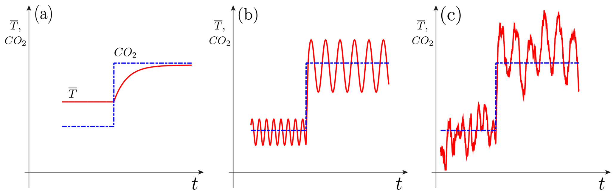
Figure 3Schematic diagram of the effects of a sudden change in atmospheric carbon dioxide (CO2) concentration (blue dashed and dotted line) on seasonally and globally averaged surface air temperature (red solid line). Climate sensitivity is shown (a) for an equilibrium model, (b) for a nonequilibrium oscillatory model, and (c) for a nonequilibrium chaotic model, possibly including random perturbations. As radiative forcing (atmospheric CO2 concentration, say) changes suddenly, global temperature () undergoes a transition. In panel (a) only the mean temperature changes, in panel (b) the mean adjusts, as it does in panel (a), but the period, amplitude, and phase of the oscillation can also decrease, increase, or stay the same, while in panel (c) the entire intrinsic variability changes as well, including the distribution of extreme events. From Ghil (2017); used with permission from the American Institute of Mathematical Sciences, under the Creative Commons Attribution license.
The figure is a highly simplified conceptual diagram of the way that anthropogenic changes in radiative forcing would change the behavior of a climate system with increasingly complex characteristics, as one proceeds from Fig. 3a through Fig. 3b and on to Fig. 3c. Therefore, neither the time, t, on the abscissa nor the CO2 concentration and temperature, , on the ordinate are labeled quantitatively in the three panels. The time we think of is years to decades, and the ranges of the CO2 concentration and correspond roughly to those expected for the difference in values between the end of the 21st century and the beginning of the 19th century. To keep things as simple as possible – but definitely not any simpler – anthropogenic changes in radiative forcing have been represented by a sudden jump in CO2 concentration, as in the Charney report.
The climate model represented in the Fig. 3a can be as simple as a forced linear, scalar, ordinary differential equation representing an energy balance model, as follows:
with λ>0, and H(t) a Heaviside function that jumps from H=0, for t≤0, to H=1, for t>0. Here and are the model's equilibrium climates for the radiative forcings before and after the jump, respectively, while λ gives the rate of exponentially approaching the new equilibrium .
The case of Fig. 3b can be seen as an idealized climate system in which the El Niño–Southern Oscillation (ENSO) would be perfectly periodic, rather than having an irregular, 2–7 year periodicity with additional periodicities and chaotic components present, as in Fig. 3c. There are no serious doubts as to the long-term mean, , after the jump being larger than the preindustrial or current mean, But, figuring out the higher moments of the long-term probability density function (pdf) after the jump is another matter entirely.
Recently, increasing attention has been paid by high-end modelers to the difficulties posed by the presence of internal variability in the climate system. For instance, Deser et al. (2020, and references therein) point to this variability's imperfect simulation and to the consequences of attempting to use models with this marked deficiency to predict future climates on multidecadal timescales.
Concerning the ENSO's distribution of extreme events, Ghil and Zaliapin (2015) investigated its dependence, in an idealized delay differential equation (DDE) model, on several model parameters. They also found that plotting the model's PBA, with respect to the seasonally periodic forcing, provided a much better understanding of the role of the seasonal cycle in the model.
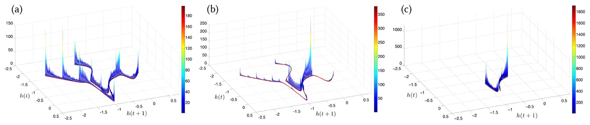
Figure 4Critical transition in extreme event distribution in an idealized El Niño–Southern Oscillation (ENSO) model. The invariant, time-dependent measure, μt, supported on the PBA of the ENSO delay differential equation (DDE) model of Tziperman et al. (1994), is plotted here via its embedding into the plane for and t≃147.64 yr and, respectively, (a) δ=0.0, (b) δ=0.01500, and (c) δ=0.015707. The red curves in the three panels represent the singular support of the measure. Reprinted with permission from Chekroun et al. (2018).
Chekroun et al. (2018) found that parameter dependence in such a DDE model can lead to a critical transition between two types of chaotic behavior which differ substantially in their distribution of extreme events. This contrast is clearly apparent in Fig. 4, and it illustrates the types of nonequilibrium climate changes suggested by Fig. 3c.
The changes in the invariant, time-dependent measure, μt, supported on this ENSO model's PBA are plotted in Fig. 4a–c as a function of the control parameter a. The change in the PBA is clearly associated with the population lying towards the ends of the elongated filaments apparent in the figure. This population represents strong, warm El Niño and cold La Niña events.
The PBA experiences a critical transition at a value, a∗; here, h(t) is the thermocline depth anomaly from seasonal depth values at the domain's eastern boundary, with t in years; and . Thus, μt(a) faithfully encrypts the disappearance of such extreme events as . Adding stochastic perturbations to the model can smooth out the transition, which might make it less drastic in high-end models and in observations. Again, the study of the model's PBA greatly facilitates the understanding of the processes involved.
4.2 Integrated assessment models (IAMs)
So-called integrated assessment models (IAMs) have been, so far, the main tool for assessing the future impact of climate change on the global economy and, even more ambitiously, on one or more regional ones (e.g., Stern, 2007; Nordhaus, 2014; Clarke et al., 2014; IPCC, 2014b; Hughes, 2019). The main purpose of IAMs is to provide reasoned scientific input into major socioeconomic and political decisions that will affect both the present and future generations of humanity, as well as planet Earth as a whole. In doing so, IAMs attempt to weigh the cost and effectiveness of competing or complementary adaptation and mitigation measures by applying various methods of cost–benefit analysis (Clarke et al., 2014; IPCC, 2014b; Hughes, 2019) and decision theory (e.g., Barnett et al., 2020, and references therein).
IAMs attempt to link major features of economy and society with the climate system and biosphere into one modeling framework, a lofty purpose that clearly has to overcome major obstacles. Some of the obstacles have to do with the complexity of the coupled system's distinct components, others with the different cultures and research styles of the scientific communities involved. Finally, the data sets necessary for estimating model parameters are short, incomplete, and often rather inaccurate. The United Nation's Intergovernmental Panel on Climate Change (IPCC) has dedicated substantial efforts over the last 3 decades to overcoming these various obstacles (IPCC, 1990, 2001, 2007, 2014a, b).
Mostly, IAMs have used both climate and economic modules that were conceived in the spirit of Fig. 3a, i.e., (i) of so-called equilibrium climate sensitivity (ECS), as studied by Charney et al. (1979) 4 decades ago, for the climate module and (ii) of general equilibrium theory (Walras, 1874/1954; Pareto, 1919; Arrow and Debreu, 1954), going back to the late 19th century, for the economic module. We have considered, in Sects. 2 and 3 above, how to formulate a more active climate module that might behave more like Fig. 3b, or even like Fig. 3c, given changes in radiative forcing induced by anthropogenic emissions of greenhouse gases and aerosols. For illustrative purposes, we will merely sketch a highly idealized counterpart of such behavior for the economic module of an IAM.
General equilibrium theory is a cornerstone of today's mainstream economics, often referred to as neoclassical economics (Aspromourgos, 1986). This theory relies heavily on equilibrium in both the labor and product markets; prices of goods and wages of labor are assumed to be flexible and to adjust so as to achieve equilibrium in the product and labor markets at all times. As a result, it is possible to maximize an intergenerational utility functional, following the planning approach of Ramsey (1928). Moreover, the mean growth of the economy (Solow, 1956) is only perturbed by exogenous shocks that lead to random fluctuations reverting to a stable equilibrium, which can be modeled by auto-regressive processes of order 1, called AR(1) processes.
The economic modules of most IAMs used so far in the IPCC process (e.g., IPCC, 2014b, and references therein) rely on general equilibrium theory and its consequences. These IAMs differ largely by the values they prescribe for various parameters; among the latter, the most important one is the discount factor, which essentially gives the future value of a currency unit versus its value today. Large differences among the value of this factor, assumed in the work of Stern (2007) versus that of Nordhaus (2014), for instance, have lead to very different conclusions about the mitigation policies recommended by these two authors.
More generally, Wagner and Weitzman (2015, among others) have emphasized how uncertainty in the climate system's dynamics could create fat-tailed distributions of potential damages, while Pindyck (2013) and Morgan et al. (2017) find existing IAMs to be of little value in providing scientific guidance for the formulation of prudent adaptation and mitigation policy. More radically, Davidson (1991) already questioned the extent to which certain types of economic uncertainties could be represented judiciously by probabilistic approaches, as has been done routinely in the IAMs' estimation of utility functionals associated with the system's future trajectories. Farmer et al. (2015) have also emphasized the need for better uncertainty estimates and better accounting for technological change and for heterogeneities in the coupled system as well as for more realistic damage functions.
More specifically, Barnett et al. (2020) have recently emphasized that the uncertainties associated with assessing the future impact of climate change, and, hence, with devising adaptation and mitigation policies, go well beyond the well-known uncertainties in the discount factor and in other parameters of either the climate or the economic module of coupled models. They suggest the following three much broader types of uncertainties:
- i.
Risk – uncertainty within a model, which involves uncertain outcomes with known probabilities
- ii.
Ambiguity – uncertainty across models, which arises from unknown weights for alternative possible models
- iii.
Misspecification – uncertainty about models, which involves unknown flaws of approximating models.
It is worth considering, in this context, the uncertainties associated with the economic counterpart of natural or intrinsic variability in the climate system; such variability is called endogenous in the economic literature. Following a parallel line of reasoning, Hallegatte (2005) argued for closed-loop climate–economy modeling, i.e., a two-way feedback interaction that also accounts for multiple timescales in both modules. We turn, therewith, to the economic part of the modeling and data analysis, as it is highly pertinent to a truly integrated way of thinking about the Earth system, including the humans that affect it more and more – whatever the exact time at which the Anthropocene (Crutzen, 2006) might have started (Lewis and Maslin, 2015).
5.1 Nonequilibrium economic models and a vulnerability paradox
There is no denying that, superimposed on overall global growth in economic activity, ups and downs are as well known as recessions and upswings. These short-term variations may appear only as small wiggles on a long-term exponential tendency of economic indicators, like gross domestic product (GDP), but they are quite severe in the individual experience of households, firms, countries, and even the world as a whole. There are two rather distinct approaches to modeling these so-called business cycles, namely the “real” business cycle (RBC) theory and the endogenous business cycle (EnBC) theory. The “real” in RBC theory refers to the fact that the theory explains macroeconomic fluctuations as the result of real productivity shocks and does not emphasize the monetary or financial aspects of the economy. A good starting point for this literature is Brock and Mirman (1972).
RBC theory is closely tied to the mainstream economics approach (Kydland and Prescott, 1982) in which the expectations of households and firms are rational, supply equals demand, and there is no involuntary unemployment. In RBC models, the fluctuations are entirely due to external, exogenous shocks, and the models' response to such shocks is purely via AR(1) processes. This theory is adopted by a very large fraction of practicing economists, and many modifications to it have tried to bring it in closer agreement with the observed behavior of real economies (e.g., Hoover, 1992). One way this approach has been criticized is that it describes the world as it ought to be, rather than how it is, and considerable controversy still exists as to its explanation of major aspects of observed macroeconomic fluctuations (e.g., Summers, 1997; Romer, 2011).
In contradistinction, EnBC theory relies on a number of heterodox – i.e., nonconformist – economic ideas, most importantly on post-Keynesian economics (Kalecki, 1935; Keynes, 1936/2018; Malinvaud, 1977). EnBC theory acknowledges at least some of the imperfections of real economies up front; in this theory, economic fluctuations are due to intrinsic processes that endogenously destabilize the economic system (Kalecki, 1935; Samuelson, 1939; Flaschel et al., 1997; Chiarella et al., 2005) and often involve delays among economic processes. Even Hayek, a leading liberal, anti-Keynesian economist, had interesting ideas on the delays between decision and implementation time in investments (Hayek, 1941/2007).
At this point it might be worth noting that, in equilibrium macroeconomic models, output is supply driven, while in nonequilibrium models it is demand driven, a feature that is inherited from the corresponding models that attempt to assess climate damage. An interesting recent example of the latter is the post-Keynesian Dynamic Ecosystem-FINance-Economy (DEFINE) model, which explicitly includes banks in addition to firms and households (Dafermos et al., 2018).
5.1.1 The nonequilibrium dynamic model of Hallegatte et al. (2008)
We present here, concisely, one particular EnBC model, and the role that active economic dynamics may have in modifying the effect of natural hazards on such an economy (Hallegatte and Ghil, 2008). The nonequilibrium dynamical model (NEDyM) of Hallegatte et al. (2008) is a neoclassical model based on the Solow (1956) model, in which equilibrium constraints associated with the clearing of goods and labor markets are replaced by dynamic relationships that involve adjustment delays. The model has eight state variables – which include production, capital, number of workers employed, wages, and prices – and the evolution of these variables is modeled by a set of ordinary differential equations. For a brief summary of the model equations, please see Groth et al. (2015a, Appendix A); the parameters and their values are listed in Hallegatte et al. (2008, Table 3).
NEDyM's main control parameter is the investment flexibility αinv, which measures the adjustment speed of investments in response to profitability signals. This parameter describes how rapidly investment can react to a profitability signal. If αinv is very large, investment soars when profits are high and collapses when profits are small, while a small αinv entails a much slower adjustment of the investment to the size of the profits. Introducing this parameter is equivalent to allocating an investment adjustment cost, as proposed by Kydland and Prescott (1982) and by Kimball (1995); these authors found that introducing adjustment costs and delays helps to match the key features of macroeconomic models to the data.
In NEDyM, for small αinv, i.e., slow adjustment, the model has a stable equilibrium, which was calibrated to the economic state of the European Union (EU-15) in 2001 (Eurostat, 2002). As the adjustment flexibility increases, this equilibrium loses its stability and undergoes a Hopf bifurcation, after which the model exhibits a stable periodic solution (Hallegatte et al., 2008).
Business cycles in NEDyM originate from the instability of the profit–investment feedback, which is quite similar to the Keynesian accelerator–multiplier effect. Furthermore, the cycles are constrained and limited in amplitude by the interplay of the following three processes: (i) a reserve army of labor effect, namely labor costs increasing when the employment rate is high, (ii) the inertia of production capacity, and (iii) the consequent inflation in goods prices when demand increases too rapidly. The model's bifurcation diagram is shown in Fig. 5.
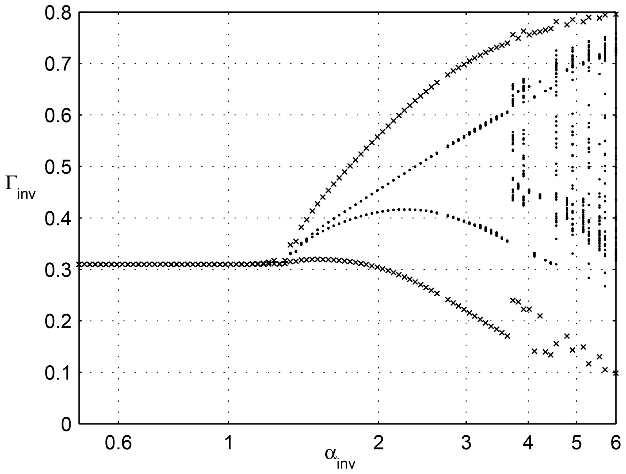
Figure 5Bifurcation diagram of a nonequilibrium dynamical model (NEDyM), showing its transitions from equilibrium to purely periodic and on to chaotic behavior. The investment parameter αinv is on the abscissa, and the investment ratio Γinv is on the ordinate. The model has a unique, stable equilibrium for low values of αinv, with Γinv≃0.3. A Hopf bifurcation occurs at αinv≃1.39, leading to a limit cycle, followed by transition to chaos at αinv≃3.8. The crosses indicate first the stable equilibrium and then the orbit's minima and maxima, while dots indicate the Poincaré intersections with the hyperplane, H=0, when the goods inventory, H, vanishes. Reproduced from Groth et al. (2015a), with permission from AGU Wiley.
For somewhat greater investment flexibility, the model exhibits chaotic behavior because a new constraint intervenes, namely limited investment capacity. In this chaotic regime, the cycles become quite irregular, with sharper recessions and recoveries of variable duration. In the present paper, we concentrate, for the sake of simplicity, on model behavior in the purely periodic regime, i.e., we have regular EnBCs but no chaos. Such periodic behavior is illustrated in Fig. 6.
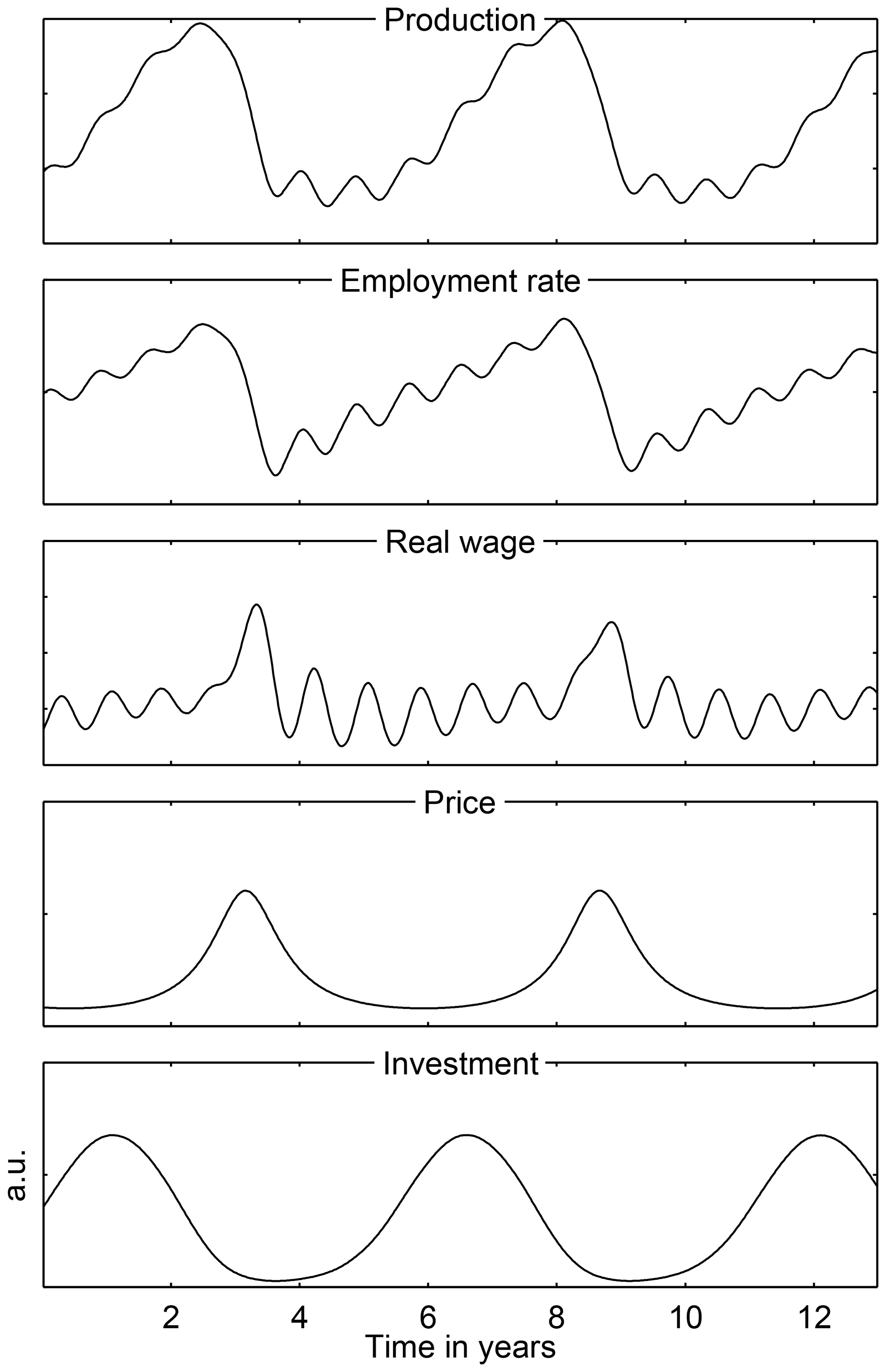
Figure 6Endogenous limit cycle behavior of NEDyM for an investment flexibility of αinv=2.5; for all other parameter values, please see Hallegatte et al. (2008, Table 3). Reproduced from Groth et al. (2015a), with permission from AGU Wiley.
The NEDyM business cycle is consistent with many stylized facts described in macroeconomic literature, such as the phasing of the distinct economic variables along the cycle, with the distinct phrases being referred to in this literature as comovements. The model also reproduces the observed asymmetry of the cycle, with recessions that are much shorter than expansions. This typical sawtooth shape of a business cycle is not well captured by RBC models, whose linear, auto-regressive character gives intrinsically symmetric behavior around the equilibrium. The amplitude of the price–wage oscillation, however, is too large in NEDyM, calling for a better calibration of the parameters and further refinements of the model.
In the setting of the 2008 economic and financial crisis, the banks' and other financial institutions' large losses clearly reduced access to credit; such a reduction very strongly affects investment flexibility. The EnBC model can thus help explain how changes in αinv can seriously perturb the behavior of the entire economic system, either by increasing or decreasing the variability in macroeconomic variables; see Fig. 5. Moreover, these losses also lead to a reduction in aggregated demand that, in turn, can lead to a reduction in economic production and a full-scale recession.
5.1.2 Regime-dependent effect of climate shocks
The immediate damage caused by a natural disaster is typically augmented by the cost of reconstruction, which is a major concern when considering the disaster's socioeconomic consequences. Reconstruction may also lead, though, to an increase in productivity by allowing for technical changes to be included in the reconstructed capital; technical changes can also sustain the demand and help economic recovery. Economic productivity may be reduced, however, during reconstruction because some vital sectors are not functional, and reconstruction investments crowd out investment into new production capacity (e.g., Hallegatte, 2016, and references therein).
In particular, Benson and Clay (2004, among others) have suggested that the overall cost of a natural disaster might depend on the preexisting economic situation. For instance, the Marmara earthquake in 1999 caused destruction that amounted to 1.5 %–3 % of Turkey's GDP; its cost in terms of production loss, however, is believed to have been fairly modest due to the fact that the country was experiencing a strong recession of −7 % of the GDP in the year before the disaster (World Bank, 2003).
To study how the state of the economy may influence the consequences of natural disasters, Hallegatte and Ghil (2008) introduced into NEDyM the disaster-modeling scheme of Hallegatte et al. (2007), in which natural disasters destroy the productive capital through a modified production function. Furthermore, to account for market frictions and constraints in the reconstruction process, the reconstruction expenditures are limited.
These authors showed that the transition from an equilibrium regime to a nonequilibrium regime can radically change the long-term response to exogenous shocks in an EnBC model. Idealized as it may be, NEDyM shows that the long-term effects of a sequence of extreme events depend upon the economy's behavior; an economy in stable equilibrium with very little, or no, flexibility (αinv≲ 0.5, see Fig. 5) is more vulnerable than a more flexible economy, albeit still at or near equilibrium (e.g., αinv≃1.0). Clearly, if investment flexibility is nil or very low, the economy is incapable of responding to the natural disasters through investment increases aimed at reconstruction; total production losses, therefore, are quite large. Such an economy behaves according to a pure Solow (1956) growth model, where the savings, and therefore the investment, ratio is constant; see Hallegatte and Ghil (2008, Table 1).
When investment can respond to profitability signals without destabilizing the economy, i.e., when αinv is nonzero but still lower than the critical bifurcation value of αinv≃1.39, the economy has greater freedom to improve its overall state and, thus, respond to productive capital influx. Such an economy is much more resilient to disasters because it can adjust its level of investment in the disaster's aftermath.
If investment flexibility, αinv, is larger than its Hopf bifurcation value, the economy undergoes periodic EnBCs, and along such a cycle, NEDyM passes through phases that differ in their stability. This, in turn, leads to a phase-dependent response to exogenous shocks and, consequently, to a phase-dependent vulnerability of the economic system, as illustrated in Fig. 7.

Figure 7Vulnerability paradox – the effect of a single natural disaster on an endogenous business cycle (EnBC). (a) The business cycle in terms of annual production, as a function of time, starting at the cycle minimum (time lag = 0). (b) Total production losses due to a disaster that instantaneously destroys 3 % of gross domestic product (GDP), shown as a function of the cycle phase in which the disaster occurs; the phase is measured as a time lag with respect to cycle minimum. A disaster occurring near the cycle's minimum (blue vertical line in both panels) causes a limited indirect production loss (blue circle), while a disaster occurring during the expansion (red vertical line in both panels) leads to a much larger loss (red circle). Figure courtesy of Andreas Groth.
5.1.3 The vulnerability paradox
A key point we wish to make in our excursion into the economical aspects of problem 10 is precisely this phase dependency of the economy's response to natural hazards.
In fact, Hallegatte and Ghil (2008) found an interesting vulnerability paradox. The indirect costs caused by extreme events during a growth phase of the economy are much higher than those that occur during a deep recession. Figure 7 illustrates this paradox by showing, in Figure 7a, a typical business cycle and, in Figure 7b, the corresponding losses for disasters hitting the economy in different phases of this cycle. The vertical lines in both panels, with blue at the end of the recession and red in the expansion phase, highlight the paradox. Hallegatte (2016, Sect. 2.2) discussed further aspects of this paradox and analogous considerations found in the much earlier work of Keynes (1936/2018).
Once noted in NEDyM behavior, this apparent paradox can be easily explained as disasters during high-growth episodes enhance preexisting disequilibria. Inventories are low and cannot compensate for the reduced production; employment is high, and hiring more employees induces wage inflation, while the producer lacks financial resources to increase investment. The opposite holds true during recessions as mobilizing investment and labor is much easier (e.g., West and Lenze, 1994).
As a consequence, production losses due to disasters that occur during expansion phases are strongly amplified, while they are reduced when the shocks occur during the recession phase. On average, however, (i) expansions last much longer than recessions in our NEDyM model as well as in reality, and (ii) amplification effects are larger than damping effects. It follows that the net effect of the cycle is strongly unfavorable to the economy, with an average production loss that is almost as large, for αinv=2.5, as for αinv=0; see again Hallegatte and Ghil (2008, Table 1).
5.2 Fluctuation–dissipation theory (FDT) and synchronization in the economic system
5.2.1 The fluctuation–dissipation conjecture
Beyond the obvious implications for disaster assessment, insurance, and other practical issues treated by Hallegatte (2016, and references therein), the findings shown schematically in Fig. 7 suggest a theoretically intriguing connection with the fluctuation–dissipation theory (FDT) in statistical mechanics. The FDT has its roots in the classical theory of many-particle systems in thermodynamic equilibrium. The idea goes back to Einstein (1905), and it is very simple; the system's return to equilibrium will be the same whether the perturbation that modified its state is due to a small external impulse or to an internal, random fluctuation. The FDT thus establishes a useful relationship between the natural and the forced fluctuations of a system (e.g., Kubo, 1966); it is a cornerstone of statistical physics and has applications in many other areas (Marconi et al., 2008, and references therein). Ghil (2019) and Ghil and Lucarini (2019) have recently reviewed FDT applications in the climate sciences, in both the classical form used for systems in equilibrium (Leith, 1975; Gritsun and Branstator, 2007), and in its more recent extensions to systems out of equilibrium, based on the Ruelle response theory (Ruelle, 1998, 2009; Lucarini, 2008; Lucarini and Gritsun, 2020).
The results in Sect. 5.1 above strongly suggest that the response to exogenous shocks of an economic system might differ from one phase of a business cycle to another. Hence, it is quite possible that the system's endogenous variability might also vary with the phase of a cycle that the system is in. More explicitly, the system's internal endogenous fluctuations may change in variance as the phase of the business cycle evolves in the same way as the exogenously driven ones do; i.e., larger “economic volatility” can be expected during expansions than during contractions of the economy. And, if this is the case, out-of-equilibrium response theory (Ruelle, 1998, 2009) may apply to economic systems in the same way that it has been found to apply to the climate system, with both the local-in-time sensitivity and volatility being phase dependent.
There is a long tradition of systematically analyzing cyclic behavior in economic data (Juglar, 1862; Kitchin, 1923; Burns and Mitchell, 1946). Yet there is no trace, as far as we could tell, of an investigation along the lines proposed herein. Hence, Groth et al. (2015a, b) set out to study the USA's macroeconomic data provided by the Bureau of Economic Analysis (BEA) for 1954–2005 to evaluate the evidence for the FDT conjecture suggested by the results reviewed in Sect. 5.1 above. The nine macroeconomic indicators these authors used were GDP, investment, consumption, employment rate (in %), total wage, change in private inventories, price, exports, and imports; see http://www.bea.gov/ (last access: 11 September 2020).
The nine indicators were each separately detrended by a Hodrick and Prescott (1997) filter, normalized by the trend values, and then collectively analyzed by using a data-adaptive multichannel singular spectrum analysis (M-SSA) filter; see Ghil et al. (2002), Alessio (2015, chap. 12) and Groth et al. (2015a, Appendix B) for details. The statistical significance of the results was carefully tested against an AR(1) null hypothesis (Allen and Smith, 1996; Ghil et al., 2002), and they are illustrated in Fig. 8.
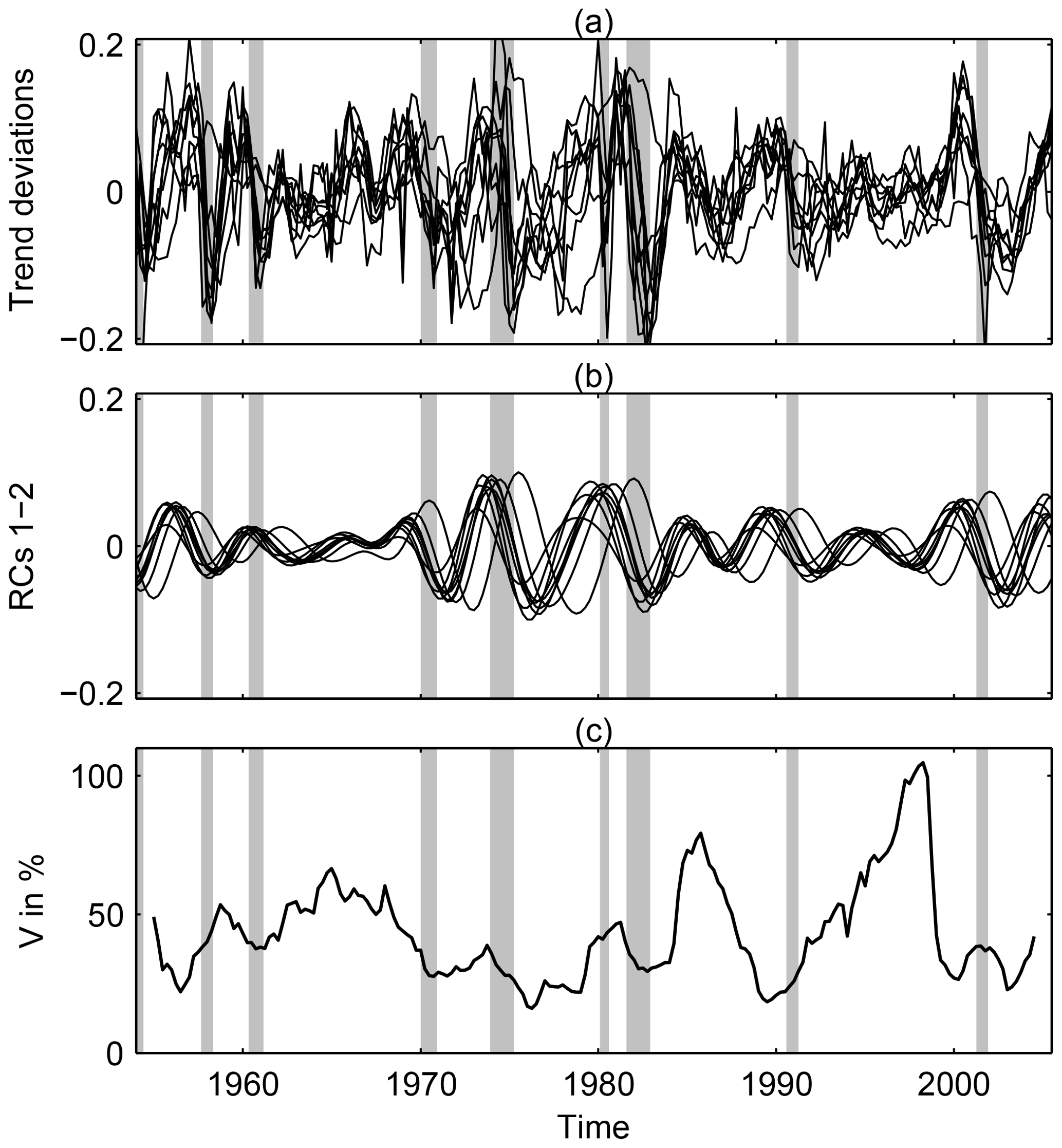
Figure 8USA business cycles and the implied fluctuation–dissipation result. Time series of nine USA macroeconomic indicators during 1954–2005. (a) Normalized trend residuals, (b) data-adaptive filtered business cycles, captured by the leading oscillatory mode of the multichannel singular spectrum analysis (M-SSA) and (c) local variance V𝒦(t) of the fluctuations. The shaded vertical bars indicate the National Bureau of Economic Research (NBER)-defined recessions (see https://www.nber.org/cycles/cyclesmain.html, last access: 11 September 2020). Reproduced from Groth et al. (2015a), with permission from AGU Wiley.
The nine detrended and normalized time series are shown in Fig. 8a, with the leading-mode pair of the joint M-SSA analysis in Fig. 8b. A simple counting of maxima and minima in Fig. 8b gives 10.5 cycles in 52 years, which agrees rather well with the NEDyM model's 5–6 year period and with the National Bureau of Economic Research's (NBER's) count of 11 cycles for the 65 year interval of 1945–2009, which yields an average period of 69 months = 5.75 years3.
In Fig. 8c the evolution in time of the local variance associated with all nine indicators is plotted, as measured over a sliding window of M=24 quarters = 6 years. It is clear that the local variance of the fluctuations, as defined in Appendix A, is consistent with the FDT hypothesis, especially over the latter part of the BEA data set; e.g., the local variance, V𝒦(t), of the fluctuations during the NBER-defined recessions of July 1981 (16 months), July 1990 (8 months), and March 2001 (8 months) is at or very near to a minimum, while substantial local maxima of V𝒦(t) are attained during the expansions in between.
5.2.2 Synchronization of economic activity
Synchronization, known in the 1970s and 1980s as entrainment (Winfree, 1980/2001; Ghil and Childress, 1987/2012), is a key feature of nonlinear oscillators that has been known since Christiaan Huygens' experiment of 1665 in which two pendulum clocks with slightly different lengths synchronized. More recently, the synchronization of chaotic oscillators has become a topic of growing interest in the physical and biological sciences (e.g., Rosenblum et al., 1996; Boccaletti et al., 2002; Pikovsky et al., 2003).
Still, while the emergence of business cycle synchronization across countries has been widely acknowledged (Artis and Zhang, 1997; Süssmuth, 2002; Kose et al., 2003) – especially in view of the ongoing globalization of economic activity – no agreement has emerged so far on basic issues like the quantification of comovements. Given the relative shortness of macroeconomic time series, efforts to apply advanced univariate analysis methods to them (e.g., de Carvalho et al., 2012; Sella et al., 2016) have provided interesting but not quite conclusive results.
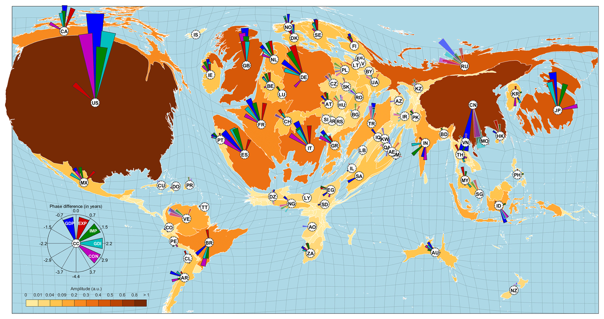
Figure 9 Leading mode of synchronized economic activity. World map of this mode's phase and amplitude relations. For each country, the relations among the variables' phase and amplitude are shown in a polar coordinate system, with the two-letter country code at the origin. The corresponding variable codes and colors of the pointers are given in the small compass inset at the lower left. Estimates for variables with missing values are indicated by transparent pointers. Phase differences are given with respect to USA GDP in a clockwise manner; i.e., positive and negative values indicate a phase that leads or lags the USA GDP, respectively. The land area of each country is proportional to its maximum amplitude over all of its variables. Reprinted from Groth and Ghil (2017), with the permission of AIP Publishing.
To overcome the difficulties posed by the simultaneous analysis of a large number of time series, Groth and Ghil (2017) applied a suitable modification of M-SSA (Groth and Ghil, 2011, 2015) to macroeconomic data from the World Development Indicators (WDI) database of the World Bank at http://databank.worldbank.org (last access: 11 September 2020). The data set extracted from the WDI database comprises five macroeconomic indicators for 104 countries, namely GDP, gross fixed capital formation (GDI, formerly gross domestic fixed investment), final consumption expenditure (CON), exports (EXP), and imports (IMP) of goods and services, with all variables in constant 2010 USD. The data were only analyzed for the 46 year interval (1970–2015) for which at least one of the indicators chosen was available for each of the 104 economies selected. The main result of this analysis is shown in Fig. 9.
The leading mode in the figure has a rough periodicity of 7–11 years, captures 73 % of the trend residual's variance, and is statistically significant according to the stringent tests of Groth and Ghil (2011, 2015, 2017). A key ingredient in the tests applied is the much larger number of data points used by the improved M-SSA methodology in examining not just GDP but a more complete set of indicators, with nine time series for Fig. 8 and five for Fig. 9.
The latter figure clearly illustrates the dominance of the USA economy over the 1970–2015 time interval, with the UK perfectly aligned on the USA indicators, while other European countries, including even the Russian Federation, lag somewhat behind. Japan is also in very good alignment with the USA, while China is in almost perfect phase opposition with it, whereas India and Indonesia follow the Chinese lead. More complicated lead-and-lag patterns are present in the much smaller economies of South America and Africa.
In this review, we have covered purely climate science problems in Sects. 2 and 3, while Sects. 4 and 5 were dedicated, respectively, to coupled climate–economy and purely economic problems. Section 2 dealt with problems 1 and 2 of Ghil (2001), and it showed progress, over the last 2 decades, in bringing more advanced nonlinear methods to bear on the issues of atmospheric low-frequency variability (LFV) and progress in extended-range forecasting, especially in the subseasonal to seasonal (S2S) range. As clearly stated by Ghil (2001), and again in Sect. 1 herein, physical sciences problems are less likely than the purely mathematical ones formulated by Hilbert (1900) to be solved to everybody's satisfaction. Figure 1 still shows a rather broad lack of consensus on the ultimate causes of atmospheric LFV.
In Sect. 3, we examined recent progress in the study of the oceans' wind-driven circulation. A key theme was studying the causes of interannual variability in the midlatitude double-gyre problem and its effect on the atmosphere above. One line of investigation dealt with providing substantial modeling and observational support to the idea that intrinsic ocean variability can have major effects on interannual atmospheric variability, such as the North Atlantic Oscillation.
Another major point touched upon in this section was the use of the theory of nonautononomous and random dynamical systems (NDS and RDS) to treat, in a fully self-consistent way, time-dependent and, possibly, random forcing by the atmosphere of a dynamically active ocean. A noteworthy finding here is the possibility of multiple modes of behavior, both quiescent and chaotic, for a given set of parameter values; see Fig. 2. Finally, a 25–30 year mode of a truly coupled ocean–atmosphere model was discussed and documented in both models and observations.
In Sect. 4.1, we emphasized the efforts made over the last 3 decades to gain greater insight into the way that climate change will affect the life of humanity on Earth and, in particular, the world economy. Figure 3 emphasizes that change in climate bears not only on the mean temperatures but also on the climate system's modes of variability and on the distribution of extreme events. Using RDS theory here is of the essence and has shown already that critical transitions between large and frequent El Niño events and much smaller ones are possible; see Fig. 4.
In Sect. 4.2, a quick introduction to integrated assessment models (IAMs) was provided, while emphasizing the equilibrium-based approach in both their climate and economic modules. The very high sensitivity to parameter values of this type of IAMs has led to rather contradictory results and, therewith, to quite opposite policy recommendations. Section 4 ends with suggesting a broader view of uncertainties than considered heretofore in studying climate change impacts on the world economy.
Section 5 addressed economic aspects of problem 10, while emphasizing nonequilibrium approaches. We first presented, for the geoscientific readership, the difference between the real business cycle (RBC) approach, based on general equilibrium theory, and the endogenous business cycle (EnBC) approach, which acknowledges the possibility of imperfect expectations and of the goods and labor markets not clearing, as well as the existence and persistence of involuntary unemployment.
In the latter spirit, we introduced in Sect. 5.1 a highly idealized nonequilibrium dynamic model (NEDyM) and showed, in Fig. 5, its bifurcation sequence, first from equilibrium to purely periodic EnBCs and on to chaotic behavior. In particular, the model exhibits relaxation oscillations with realistically fast contractions and slow expansions; e.g., the mean duration of the USA economy's contractions for the post-World War II (WWII) interval 1945–2009, with 11 cycles, was of 11.1 months, while expansions lasted, on average, 58.4 months4. Such sawtooth behavior cannot be captured by RBC models in which shocks regress to the mean in AR(1) fashion independently of the sign of the shock.
The existence of endogenous variability gives rise to a vulnerability paradox, illustrated in Fig. 7, with an exogenous shock producing higher losses during an expansion than during a recession. This asymmetry in the response, when integrated over several cycles, produces a net effect that differs from that shown by IAMs based on general equilibrium theory and the so-called Ramsey (1928) planners deduced from that theory.
The vulnerability paradox of Fig. 7 thus led us to the FDT conjecture and its very careful, but still tentative, verification with USA macroeconomic data in Fig. 8. NEDyM, though, is but a highly idealized aggregate macroeconomic model. It would, therefore, be highly desirable to see such FDT results being reproduced in much more detailed, agent-based models (e.g., Epstein and Axtell, 1996; Bouchaud, 2013; Mazzoli et al., 2019, and references therein). Likewise, producing figures along the lines of Fig. 8 herein with other methods and other data sets would help invalidate, according to Popper (2005), the present conclusions or, on the contrary, show some consistency with them.
In Sect. 5.2, we turned to the fluctuation–dissipation conjecture suggested by the above vulnerability paradox. To wit, internal endogenous fluctuations are likely to change in variance with the phase of the business cycle in the same way as the exogenously driven ones; i.e., larger volatility can be expected during expansions than during contractions of the economy. This conjecture was clearly confirmed by the results reproduced in Fig. 8 of an investigation into USA macroeconomic indicators. Consequently, the out-of-equilibrium response theory (Ruelle, 1998, 2009; Lucarini, 2008) may apply to economic systems in the way that it has been found to apply to the climate system, with both local-in-time sensitivity and volatility being phase dependent.
The FDT result captured by Figs. 7 and 8 holds, therewith, great promise for the study of an economic entity's sensitivity to environmental and to economic, political, or financial shocks. In general, the usefulness of such a result (Kubo, 1966; Leith, 1975) lies in the fact that one has a much longer record of internal fluctuations than of responses to shocks; see also Ghil (2019, Sect. 5.2) and Ghil and Lucarini (2019, Sect. IV.E). Thus, the response to the latter – e.g., the decay time of an exogenous shock's effect on the system – can be determined from the system's typical lag-autocorrelation time.
Section 5 concluded by reviewing a query into the existence of a worldwide synchronization of economic activity, resulting in a positive conclusion (see Fig. 9 herein). Synchronization, though, depends sensitively on the coupling parameters between chaotic oscillators (e.g., Colon and Ghil, 2017; Duane et al., 2017, and references therein). So far, the main concerns of IAM-based investigations of the overall worldwide economic effects of climate change – and even those of specific studies of more localized economic effects – of extreme climatic and other natural events have focused on physical losses of economic productivity. Sensitive dependence of synchronization on parameter values suggests that more subtle, but still calamitous, productivity losses could arise from climatically driven changes in the world economic activity's degree of synchronization.
Finally, we note that significant steps have been taken of late to achieve insights into an even broader system, beyond climate and the economy, to encompass sociological aspects of climate change impacts as well (e.g., Motesharrei et al., 2014, 2016). Useful pointers in the direction of dynamic modeling of sociological problems can be found in the fairly obvious analogy between the latter and ecological ones, as noted by Samuelson (1971), May et al. (2008), and Colon et al. (2015), among others.
Covering these developments would require expanding the present review much further, which is not in the cards at this time. Still, the answer to problem 10 of Ghil (2001), namely “Can we achieve enlightened climate control of our planet by the end of the century?”, does require a complete understanding of the behavior of such a coupled socioeconomic–physical–biological system, along with a deeper understanding of who “we” are and who exercises the control.
Given the importance of the FDT conjecture for studying the economic system, we provide herein a quick introduction to the local variance concept used in Sect. 5.1 and illustrated in Fig. 8c. Please see Ghil et al. (2002) and Groth et al. (2015a), for the precise definitions and equations used in the M-SSA methodology, and Groth et al. (2015b), for the details of the statistical significance tests applied to the BEA data set.
Plaut and Vautard (1994) introduced the concept of local variance fraction V𝒦(t) as follows:
which quantifies the fraction of the total variance that is described by a subset 𝒦 of SSA principal components (PCs; i.e., temporal PCs or T-PCs) in a sliding window of length M=24 quarters. The T-PCs here are considered as being centered, i.e., starting at M∕2 and ending at , and D=9 is the dimension of the phase space into which the macroeconomic indicators are embedded (see Groth et al., 2015b, Sect. 2.2 and 2.3). Here N is the total length of the time series, with N=52 years × 4 quarters = 208 data points for each time series.
The leading oscillatory mode plotted in Fig. 8b corresponds to , and it is considered as the signal, while the complementary set, , is identified with the fluctuations whose evolving variance we wish to track. More precisely, a total of eigenvalues in the M-SSA decomposition captures 99 % of the BEA data set's total variance. Hence, the local variance plotted in Fig. 8c corresponds to .
Data sources are as follows: (1) USA macroeconomic indicators at http://www.bea.gov (last access: 14 September 2020); (2) historical data on past USA recessions at https://www.nber.org/cycles/cyclesmain.html (last access: 14 September 2020); (3) macroeconomic data from the World Development Indicators (WDI) database of the World Bank at http://databank.worldbank.org (last access: 14 September 2020); and (4) National Bureau of Economic Research (NBER)-defined recessions at https://www.nber.org/cycles/cyclesmain.html (last access: 14 September 2020).
The author declares that there is no conflict of interest.
This article is part of the special issue “Centennial issue on nonlinear geophysics: accomplishments of the past, challenges of the future”. It is not associated with a conference.
It is a pleasure to thank Daniel Schertzer for the invitation to write an update of the Ghil (2001) paper for the “Centennial issue on nonlinear geophysics: accomplishments of the past, challenges of the future” of the Nonlinear Processes in Geophysics journal. Sections 2 and 3 of this review have benefited from interaction with many colleagues from the climate science community over the years; quite a few of them have been acknowledged recently in Ghil (2019) and in Ghil and Lucarini (2019). In connection with Sects. 4 and 5, it is a great pleasure to thank Michael D. Barnett, Enrico Biffis, William A. Brock, Erik Chavez, Carl Chiarella, David Claessen (deceased 2018), Célian Colon, Barbara Coluzzi, Patrice Dumas, Andreas Groth, Stéphane Hallegatte, Lars P. Hansen, Jean-Charles Hourcade, Maria Nikolaidi, Marc Sadler, Lisa Sela, Pietro Terna, Gianna Vivaldo, and Gérard Weisbuch for all they taught me about economics and its modeling. I am deeply indebted to William A. Brock, Célian Colon, Maria Nikolaidi, and Pietro Terna for enlightening comments on a draft of this paper, especially regarding Sects. 4 and 5. Two anonymous reviewers and Valerio Lucarini have made highly constructive and helpful suggestions that have further improved the presentation. This paper is Tipping Points in the Earth System (TiPES) contribution no. 19; the TiPES project has received funding from the European Union's Horizon 2020 research and innovation program (grant no. 820970). Work on this paper has also been supported by the EIT Climate-KIC; EIT Climate-KIC is supported by the European Institute of Innovation and Technology (EIT), a body of the European Union.
This research has been supported by the European Union's Horizon 2020 re-search and innovation program (TiPES, grant no. 820970) and the EIT Climate-KIC (European Institute of Innovation and Technology), a body of the European Union.
This paper was edited by Stéphane Vannitsem and reviewed by two anonymous referees.
Alessio, S. M.: Digital Signal Processing and Spectral Analysis for Scientists: Concepts and Applications, Springer Science and Business Media, https://doi.org/10.1007/978-3-319-25468-5, 2015. a
Alkhayuon, H., Ashwin, P., Jackson, L. C., Quinn, C., and Wood, R. A.: Basin bifurcations, oscillatory instability and rate-induced thresholds for AMOC in a global oceanic box model, arXiv [preprint], arXiv:1901.10111, 29 January 2019. a
Allen, M. R.: Liability for climate change, Nature, 421, 891–892, 2003. a
Allen, M. R. and Smith, L. A.: Monte Carlo SSA: Detecting irregular oscillations in the presence of colored noise, J. Climate, 9, 3373–3404, 1996. a
Arrow, K. J. and Debreu, G.: Existence of an equilibrium for a competitive economy, Econometrica, 22, 265–290, 1954. a
Artis, M. J. and Zhang, W.: International business cycles and the ERM: is there a European business cycle?, Int. J. Financ. Econ., 2, 1–16, 1997. a
Aspromourgos, T.: On the origins of the term `neoclassical', Camb. J. Econ., 10, 265–270, 1986. a
Barnett, M., Brock, W., and Hansen, L. P.: Pricing uncertainty induced by climate change, Rev. Financ. Stud., 33, 1024–1066, 2020. a, b
Bengtsson, L., Ghil, M., and Källén, E.: Dynamic Meteorology: Data Assimilation Methods, Springer, Berlin/Heidelberg, Germany/New York, USA, 1981. a
Benson, C. and Clay, E.: Understanding the Economic and Financial Impacts of Natural Disasters, The World Bank, Washington, DC, USA, 2004. a
Berloff, P., Hogg, A. M., and Dewar, W.: The turbulent oscillator: A mechanism of low-frequency variability of the wind-driven ocean gyres, J. Phys. Oceanogr., 37, 2363–2386, 2007. a
Boccaletti, S., Kurths, J., Osipov, G., Valladares, D. L., and Zhou, C. S.: The synchronization of chaotic systems, Phys. Rep., 366, 1–101, https://doi.org/10.1016/s0370-1573(02)00137-0, 2002. a
Bódai, T. and Tél, T.: Annual variability in a conceptual climate model: Snapshot attractors, hysteresis in extreme events, and climate sensitivity, Chaos, 22, 023110, https://doi.org/10.1063/1.3697984, 2012. a
Bódai, T., Lucarini, V., and Lunkeit, F.: Can we use linear response theory to assess geoengineering strategies?, Chaos, 30, 023124, https://doi.org/10.1063/1.5122255, 2020. a
Bouchaud, J.-P.: Crises and collective socio-economic phenomena: Simple models and challenges, J. Stat. Phys., 151, 567–606, https://doi.org/10.1007/s10955-012-0687-3, 2013. a
Brock, W. and Mirman, L.: Optimal growth under uncertainty, J. Econ. Theory, 4, 479–513, 1972. a
Burns, A. F. and Mitchell, W. C.: Measuring Business Cycles, Tech. rep., National Bureau of Economic Research, Cambridge, Mass., USA, 1946. a
Carrassi, A., Bocquet, M., Hannart, A., and Ghil, M.: Estimating model evidence using data assimilation, Q. J. Roy. Meteor. Soc., 143, 866–880, 2017. a
Cessi, P.: The global overturning circulation, Annu. Rev. Mar. Sci., 11, 249–270, 2019. a
Charney, J. G. and DeVore, J. G.: Multiple flow equilibria in the atmosphere and blocking, J. Atmos. Sci., 36, 1205–1216, 1979. a
Charney, J. G., Arakawa, A., Baker, D. J., Bolin, B., Dickinson, R. E., Goody, R. M., Leith, C. E., Stommel, H. M., and Wunsch, C. I.: Carbon Dioxide and Climate: A Scientific Assessment, National Academy of Sciences, Washington, DC, 1979. a, b
Chavez, M., Ghil, M., and Urrutia-Fucugauchi, J. (Eds.): Extreme Events: Observations, Modeling, and Economics, vol. 214 of Geophysical Monographs, John Wiley and Sons, Hoboken, NJ, USA, 2015. a
Chekroun, M. D., Simonnet, E., and Ghil, M.: Stochastic climate dynamics: random attractors and time-dependent invariant measures, Physica D, 240, 1685–1700, https://doi.org/10.1016/j.physd.2011.06.005, 2011. a
Chekroun, M. D., Ghil, M., and Neelin, J. D.: Pullback attractor crisis in a delay differential ENSO model, in: Advances in Nonlinear Geosciences, edited by: Tsonis, A., Springer, Cham, Switzerland, 1–33, 2018. a, b
Chiarella, C., Flaschel, P., and Franke, R.: Foundations for a Disequilibrium Theory of the Business Cycle, Cambridge University Press, Cambridge, UK, 2005. a
Clarke, L. E., Jiang, K., Akimoto, K., Babiker, M., Blanford, G. J., Fisher-Vanden, K., Hourcade, J.-C., Krey, V., Kriegler, E., Loschel, A., McCollum, K., Paltsev, S., Rose, S., Shukla, P. R., Tavoni, M., van der Zwaan, B., and van Vuuren, D. P.: Assessing transformation pathways, Chapter 6, in: Climate Change 2014: Mitigation of Climate Change. Contribution of Working Group III to the Fifth Assessment Report of the Intergovernmental Panel on Climate Change, edited by: Edenhofer, O., Pichs-Madruga, R., Sokona, Y., Farahani, E., Kadner, S., Seyboth, K., Adler, A., Baum, I., Brunner, S., Eickemeier, P., Kriemann, B., Savolainen, J., Schlömer, S., von Stechow, C., Zwickel, T., and Minx, J. C., Cambridge University Press, Cambridge, UK, 2014. a, b
Colon, C. and Ghil, M.: Economic networks: Heterogeneity-induced vulnerability and loss of synchronization, Chaos, 27, 126703, https://doi.org/10.1063/1.5017851, 2017. a
Colon, C., Claessen, D., and Ghil, M.: Bifurcation analysis of an agent-based model for predator–prey interactions, Ecol. Model., 317, 93–106, 2015. a
Crutzen, P. J.: The “anthropocene”, in: Earth System Science in the Anthropocene, pp. 13–18, Springer, 2006. a
Cvitanović, P. and Eckhardt, B.: Periodic-orbit quantization of chaotic systems, Phys. Rev. Lett., 63, 823–826, 1989. a
Dafermos, Y., Nikolaidi, M., and Galanis, G.: Climate change, financial stability and monetary policy, Ecol. Econ., 152, 219–234, 2018. a
Davidson, P.: Is probability theory relevant for uncertainty? A Post Keynesian perspective, J. Econ. Perspect., 5, 129–143, https://doi.org/10.1257/jep.5.1.129, 1991. a
de Carvalho, M., Rodrigues, P. C., and Rua, A.: Tracking the US business cycle with a singular spectrum analysis, Econ. Lett., 114, 32–35, https://doi.org/10.1016/j.econlet.2011.09.007, 2012. a
Deser, C., Lehner, F., Rodgers, K. B., Ault, T., Delworth, T. L., DiNezio, P. N., Fiore, A., Frankignoul, C., Fyfe, J. C., Horton, D. E., et al.: Insights from Earth system model initial-condition large ensembles and future prospects, Nat. Clim. Change, 10, 277–286, 2020. a
Dijkstra, H. A. and Ghil, M.: Low-frequency variability of the large-scale ocean circulation: A dynamical systems approach, Rev. Geophys., 43, RG3002, https://doi.org/10.1029/2002RG000122, 2005. a
Duane, G. S., Grabow, C., Selten, F., and Ghil, M.: Introduction to focus issue: Synchronization in large networks and continuous media-data, models, and supermodels, Chaos, 27, 126601, https://doi.org/10.1063/1.5018728, 2017. a
Einstein, A.: Über die von der molekularkinetischen Theorie der Wärme geforderte Bewegung von in ruhenden Flüssigkeiten suspendierten Teilchen, Ann. Phys., 322, 549–560, reprinted in: Investigations on the Theory of the Brownian Movement, five articles by A. Einstein, edited by: Furth, R., transleted by: Cowper, A. D., 1956, Dover Publ., New York, 122 pp., 1905. a
Epstein, J. M. and Axtell, R.: Growing Artificial Societies: Social Science from the Bottom Up, Brookings Institution Press, Washington, DC, USA, 1996. a
Eurostat: Economic Portrait of the European Union 2001, Tech. rep., European Commission, Brussels, 2002. a
Farmer, J. D., Hepburn, C., Mealy, P., and Teytelboym, A.: A third wave in the economics of climate change, Environmental and Resource Economics, 62, 329–357, 2015. a
Feliks, Y., Ghil, M., and Simonnet, E.: Low-frequency variability in the midlatitude atmosphere induced by an oceanic thermal front, J. Atmos. Sci., 61, 961–981, 2004. a
Feliks, Y., Ghil, M., and Simonnet, E.: Low-frequency variability in the midlatitude baroclinic atmosphere induced by an oceanic thermal front, J. Atmos. Sci., 64, 97–116, 2007. a
Flaschel, P., Franke, R., Semmler, W., Day, R. H., et al.: Dynamic Macroeconomics: Instability, Fluctuation, and Growth in Monetary Economies, MIT Press, Cambridge, Mass., USA, 1997. a
Frankcombe, L. M. and Dijkstra, H. A.: The role of Atlantic-Arctic exchange in North Atlantic multidecadal climate variability, Geophys. Res. Lett., 38, L16603, https://doi.org/10.1029/2011GL048158, 2011. a
Ghil, M.: Hilbert problems for the geosciences in the 21st century, Nonlin. Processes Geophys., 8, 211–211, https://doi.org/10.5194/npg-8-211-2001, 2001. a, b, c, d, e, f, g, h, i, j, k
Ghil, M.: The wind-driven ocean circulation: Applying dynamical systems theory to a climate problem, Discrete Cont. Dyn.-A, 37, 189–228, https://doi.org/10.3934/dcds.2017008, 2017. a, b, c
Ghil, M.: A century of nonlinearity in the geosciences, Earth and Space Science, 6, 1007–1042, https://doi.org/10.1029/2019EA000599, 2019. a, b, c, d, e
Ghil, M. and Childress, S.: Topics in Geophysical Fluid Dynamics: Atmospheric Dynamics, Dynamo Theory, and Climate Dynamics, Springer Science+Business Media, Berlin, Heidelberg, Reissued in pdf, 2012, 1987/2012. a, b
Ghil, M. and Lucarini, V.: The physics of climate variability and climate change, arXiv [preprint], arXiv:1910.00583, 1 October 2019. a, b, c, d, e, f, g
Ghil, M. and Malanotte-Rizzoli, P.: Data assimilation in meteorology and oceanography, Adv. Geophys., 33, 141–266, 1991. a
Ghil, M. and Robertson, A. W.: ”Waves” vs. ”particles” in the atmosphere's phase space: A pathway to long-range forecasting?, P. Natl. Acad. Sci. USA, 99, 2493–2500, 2002. a
Ghil, M. and Zaliapin, I.: Understanding ENSO variability and its extrema: A delay differential equation approach, Chapter 6, in: Extreme Events: Observations, Modeling and Economics, edited by: Chavez, M., Ghil, M., and Urrutia-Fucugauchi, J., Geophysical Monographs, Wiley Online Library, 214, 63–78, 2015. a
Ghil, M., Allen, M. R., Dettinger, M. D., Ide, K., Kondrashov, D., Mann, M. E., Robertson, A. W., Saunders, A., Tian, Y., Varadi, F., and Yiou, P.: Advanced spectral methods for climatic time series, Rev. Geophys., 40, 31–341, https://doi.org/10.1029/2000RG000092, 2002. a, b, c
Ghil, M., Chekroun, M. D., and Simonnet, E.: Climate dynamics and fluid mechanics: Natural variability and related uncertainties, Physica D, 237, 2111–2126, https://doi.org/10.1016/j.physd.2008.03.036, 2008. a, b
Ghil, M., Yiou, P., Hallegatte, S., Malamud, B. D., Naveau, P., Soloviev, A., Friederichs, P., Keilis-Borok, V., Kondrashov, D., Kossobokov, V., Mestre, O., Nicolis, C., Rust, H. W., Shebalin, P., Vrac, M., Witt, A., and Zaliapin, I.: Extreme events: dynamics, statistics and prediction, Nonlin. Processes Geophys., 18, 295–350, https://doi.org/10.5194/npg-18-295-2011, 2011. a
Ghil, M., Groth, A., Kondrashov, D., and Robertson, A. W.: Extratropical sub-seasonal–to–seasonal oscillations and multiple regimes: The dynamical systems view, Chap. 6, in: The Gap Between Weather and Climate Forecasting: Sub-Seasonal to Seasonal Prediction, edited by: Robertson, A. W. and Vitart, F., Elsevier, Amsterdam, 119–142, 2018. a, b, c, d
Gill, A. E.: Atmosphere-Ocean Dynamics, Academic Press, New York, USA, 1982. a
Gilmore, R.: Topological analysis of chaotic dynamical systems, Rev. Mod. Phys., 70, 1455–1529, 1998. a
Gritsun, A. and Branstator, G.: Climate response using a three-dimensional operator based on the fluctuation–dissipation theorem, J. Atmos. Sci., 64, 2558–2575, https://doi.org/10.1175/JAS3943.1, 2007. a
Groth, A. and Ghil, M.: Multivariate singular spectrum analysis and the road to phase synchronization, Phys. Rev. E, 84, 036206, https://doi.org/10.1103/PhysRevE.84.036206, 2011. a, b
Groth, A. and Ghil, M.: Monte Carlo singular spectrum analysis (SSA) revisited: Detecting oscillator clusters in multivariate datasets, J. Climate, 28, 7873–7893, https://doi.org/10.1175/JCLI-D-15-0100.1, 2015. a, b
Groth, A. and Ghil, M.: Synchronization of world economic activity, Chaos, 27, 127002, https://doi.org/10.1063/1.5001820, 2017. a, b, c
Groth, A., Feliks, Y., Kondrashov, D., and Ghil, M.: Interannual variability in the North Atlantic ocean's temperature field and its association with the wind stress forcing, J. Climate, 30, 2655–2678, 2017. a
Groth, A., Dumas, P., Ghil, M., and Hallegatte, S.: Impacts of natural disasters on a dynamic economy, Chap. 19, in: Extreme Events: Observations, Modeling and Economics, edited by: Chavez, M., G. M. and Urrutia-Fucugauchi, J., Geophysical Monographs, 214, 343–359, 2015a. a, b, c, d, e, f, g
Groth, A., Ghil, M., Hallegatte, S., and Dumas, P.: The role of oscillatory modes in US business cycles, OECD Journal: Journal of Business Cycle Measurement and Analysis, 2015, 63–81, 2015b. a, b, c
Hallegatte, S.: The long time scales of the climate–economy feedback and the climatic cost of growth, Environ. Model. Assess., 10, 277–289, 2005. a
Hallegatte, S.: Natural Disasters and Climate Change: An Economic Perspective, Springer, Berlin, Heidelberg, Germany, Dordrecht, the Netherlands, and New York City, USA, 2016. a, b, c
Hallegatte, S. and Ghil, M.: Natural disasters impacting a macroeconomic model with endogenous dynamics, Ecol. Econ., 68, 582–592, https://doi.org/10.1016/j.ecolecon.2008.05.022, 2008. a, b, c, d, e
Hallegatte, S., Hourcade, J.-C., and Dumas, P.: Why economic dynamics matter in assessing climate change damages: Illustration on extreme events, Ecol. Econ., 62, 330–340, https://doi.org/10.1016/j.ecolecon.2006.06.006, 2007. a
Hallegatte, S., Ghil, M., Dumas, P., and Hourcade, J.-C.: Business cycles, bifurcations and chaos in a neo-classical model with investment dynamics, J. Econ. Behav. Organ., 67, 57–77, https://doi.org/10.1016/j.jebo.2007.05.001, 2008. a, b, c, d, e
Hannart, A., Carrassi, A., Bocquet, M., Ghil, M., Naveau, P., Pulido, M., Ruiz, J., and Tandeo, P.: DADA: data assimilation for the detection and attribution of weather and climate-related events, Climatic Change, 136, 155–174, 2016a. a
Hannart, A., Pearl, J., Otto, F. E. L., Naveau, P., and Ghil, M.: Causal counterfactual theory for the attribution of weather and climate-related events, B. Am. Meteorol. Soc., 97, 99–110, 2016b. a, b, c, d, e, f
Hasselmann, K.: Stochastic climate models. I: Theory, Tellus, 28, 473–485, 1976. a
Hawkins, E., Smith, R. S., Allison, L. C., Gregory, J. M., Woollings, T. J., Pohlmann, H., and Cuevas, B.: Bistability of the Atlantic overturning circulation in a global climate model and links to ocean freshwater transport, Geophys. Res. Lett., 38, L10605, https://doi.org/10.1029/2011GL047208, 2011. a
Hayek, F. A.: The Pure Theory of Capital; first published by Macmillan and Co. in 1941, vol. 12 of The Collected Works of F. A. Hayek, University of Chicago Press, Chicago, Ill., USA, 1941/2007. a
Held, I. M.: The gap between simulation and understanding in climate modeling, B. Am. Meteorol. Soc., 86, 1609–1614, https://doi.org/10.1175/bams-86-11-1609, 2005. a
Hilbert, D.: Mathematische Probleme, Göttinger Nachrichten, 253–297, see also Archiv d. Mathematik u. Physik, 3, 44–63 and 213–237, 1901, French transl. by: Laugel, M. L., Sur les probèmes futurs des mathématiques, in Comptes Rendus du 2ème Congrès International des Mathématiciens, 58–114, Gauthier-Villars, Paris, 1902, Engl. transl. by: Winton Newson, M., B. Am. Math. Soc., 8, 437–479, 1902, 1900. a, b, c
Hodrick, R. J. and Prescott, E. C.: Postwar US business cycles: an empirical investigation, J. Money Credit Bank., 29, 1–16, 1997. a
Hoover, K.: The New Classical Macroeconomics, Edward Elgar Publishing, see also Kevin D. Hoover, The New Classical Macroeconomics, in The Library of Economics and Liberty, available at: https://www.econlib.org/library/Enc/NewClassicalMacroeconomics.html (last access: 14 September 2020), 1992. a
Hughes, B. B.: International Futures: Building and Using Global Models, Academic Press, Cambridge, Mass., USA, 2019. a, b
IPCC: Climate Change: The IPCC Scientific Assessment, Report Prepared for Intergovernmental Panel on Climate Change by Working Group I., edited by: Houghton, J. T., Jenkins, G. J., and Ephraums, J. J., Cambridge University Press, Cambridge, UK, 365+xxxix pp., 1990. a, b
IPCC: Climate Change 2001: The Scientific Basis, Contribution of Working Group I to the Third Assessment Report of the Intergovernmental Panel on Climate Change, edited by: Houghton, J. T., Cambridge University Press, Cambridge, UK, 2001. a, b
IPCC: Climate Change 2007 – The Physical Science Basis: Working Group I Contribution to the Fourth Assessment Report of the IPCC, edited by: Solomon, S., Manning, M., Marquis, M., and Qin, D., Cambridge University Press, Cambridge, UK and New York, NY, USA, 2007. a, b
IPCC: Climate Change 2013: The Physical Science Basis, Contribution of Working Group I to the Fifth Assessment Report of the Intergovernmental Panel on Climate Change, edited by: Stocker, T. F., Qin, D., Plattner, G.-K., Tignor, M., Allen, S. K., Boschung, J., Nauels, A., Xia, Y., Bex, V., and Midgley, P. M., Cambridge University Press, Cambridge, https://doi.org/10.1017/cbo9781107415324, 2014a. a, b, c
IPCC: Climate Change 2014: Synthesis Report, Contribution of Working Groups I, II and III to the Fifth Assessment Report of the Intergovernmental Panel on Climate Change, edited by: Pachauri, R. K. and Meyer, L. A., Intergovernmental Panel on Climate Change, Geneva, Switzerland, 151 pp., 2014b. a, b, c, d, e, f
Itoh, H. and Kimoto, M.: Chaotic itinerancy with preferred transition routes appearing in an atmospheric model, Physica D, 109, 274–292, https://doi.org/10.1016/s0167-2789(97)00064-x, 1997. a
Jiang, S., Jin, F.-F., and Ghil, M.: Multiple equilibria and aperiodic solutions in a wind-driven double-gyre, shallow-water model, J. Phys. Oceanogr., 25, 764–786, 1995. a
Juglar, C.: Des Crises commerciales et leur retour périodique en France, en Angleterre, et aux Etats Unis, Guillaumin, Paris, 1862. a
Kalecki, M.: A macrodynamic theory of business cycles, Econometrica, 3, 327–344, 1935. a, b
Kalnay, E.: Atmospheric Modeling, Data Assimilation and Predictability, Cambridge University Press, Cambridge, UK, 2003. a, b
Keynes, J. M.: The General Theory of Employment, Interest, and Money, first published by Palgrave Macmillan in 1936, Springer, Berlin, Heidelberg, Germany, Dordrecht, the Netherlands, and New York City, USA, 1936/2018. a, b
Kimball, M. S.: The quantitative analytics of the basic neomonetarist model, J. Money Credit Bank., 27, 1241–1277, 1995. a
Kimoto, M. and Ghil, M.: Multiple flow regimes in the Northern Hemisphere winter. Part I: Methodology and hemispheric regimes, J. Atmos. Sci., 50, 2625–2643, 1993a. a
Kimoto, M. and Ghil, M.: Multiple flow regimes in the Northern Hemisphere winter. Part II: Sectorial regimes and preferred transitions, J. Atmos. Sci., 50, 2645–2673, 1993b. a
Kitchin, J.: Cycles and Trends in Economic Factors, Rev. Econ. Statistics, 5, 10–16, https://doi.org/10.2307/1927031, 1923. a
Kolmogoroff, A.: Grundbegriffe der Wahrscheinlichkeitsrechnung, Springer Nature Switzerland AG, https://doi.org/10.1007/978-3-642-49888-6, 1933, reissued in 2019. a
Kondrashov, D., Kravtsov, S., and Ghil, M.: Empirical mode reduction in a model of extratropical low-frequency variability, J. Atmos. Sci., 63, 1859–1877, 2006. a, b
Kose, M. A., Otrok, C. M., and Whiteman, C. H.: International business cycles: world, region, and country-specific factors, Am. Econ. Rev., 93, 1216–1239, https://doi.org/10.1257/000282803769206278, 2003. a
Kubo, R.: The fluctuation-dissipation theorem, Rep. Prog. Phys., 29, 255–284, 1966. a, b
Kydland, F. E. and Prescott, E. C.: Time to build and aggregate fluctuations, Econometrica, 50, 1345–1370, 1982. a, b
Legras, B. and Ghil, M.: Persistent anomalies, blocking, and variations in atmospheric predictability, J. Atmos. Sci., 42, 433–471, 1985. a, b
Leith, C. E.: Climate response and fluctuation dissipation, J. Atmos. Sci., 32, 2022–2026, https://doi.org/10.1175/1520-0469(1975)032{<}2022:CRAFD{>}2.0.CO;2, 1975. a, b
Lewis, S. L. and Maslin, M. A.: Defining the anthropocene, Nature, 519, 171–180, 2015. a
Lindzen, R. S.: Stationary planetary waves, blocking, and interannual variability, Adv. Geophys., 29, 251–273, https://doi.org/10.1016/s0065-2687(08)60042-4, 1986. a
Lorenz, E. N.: The Nature and Theory of the General Circulation of the Atmosphere, World Meteorological Organization, Geneva, Switzerland, 1967. a
Lorenz, E. N.: Three approaches to atmospheric predictability, B. Am. Meteorol. Soc., 50, 345–349, 1969. a
Lucarini, V.: Response theory for equilibrium and non-equilibrium statistical mechanics: Causality and generalized Kramers-Kronig relations, J. Stat. Phys., 131, 543–558, https://doi.org/10.1007/s10955-008-9498-y, 2008. a, b
Lucarini, V. and Gritsun, A.: A new mathematical framework for atmospheric blocking events, Clim. Dynam., 54, 575–598, 2020. a, b, c, d
Lucarini, V., Faranda, D., de Freitas, A. C. G. M. M., de Freitas, J. M. M., Holland, M., Kuna, T., Nicol, M., Todd, M., and Vaienti, S.: Extremes and Recurrence in Dynamical Systems, Wiley, Hoboken, NJ, USA, 2016. a
Malinvaud, E.: The Theory of Unemployment Reconsidered, Blackwell, Oxford, 1977. a
Malone, T. F., Houghton, H. G., Byers, H. R., Landsberg, H. E., Wexler, H., Haurwitz, B., Spilhaus, A. F., and Willett, H. C. (Eds.): Compendium of Meteorology, American Meteorological Society, reissued in pdf by Springer, Berlin, Heidelberg, Germany, Dordrecht, the Netherlands, and New York City, USA, 2016, 1951/1955/2016. a
Marconi, U. M. B., Puglisi, A., Rondoni, L., and Vulpiani, A.: Fluctuation-dissipation: Response theory in statistical physics, Phys. Rep., 461, 111–195, 2008. a
Marshall, J. and Molteni, F.: Toward a dynamical understanding of atmospheric weather regimes, J. Atmos. Sci., 50, 1993–2014, 1993. a
May, R. M., Levin, S. A., and Sugihara, G.: Complex systems: Ecology for bankers, Nature, 451, 893–895, 2008. a
Mazzoli, M., Morini, M., and Terna, P.: Rethinking Macroeconomics with Endogenous Market Structure, Cambridge University Press, Cambridge, UK, 2019. a
Minobe, S., Kuwano-Yoshida, A., Komori, N., Xie, S.-P., and Small, R. J.: Influence of the Gulf Stream on the troposphere, Nature, 452, 206–209, 2008. a
Morgan, M. G., Vaishnav, P., Dowlatabadi, H., and Azevedo, I. L.: Rethinking the social cost of carbon dioxide, Issues Sci. Technol., 33, 43–50, 2017. a
Motesharrei, S., Rivas, J., and Kalnay, E.: Human and nature dynamics (HANDY): Modeling inequality and use of resources in the collapse or sustainability of societies, Ecol. Econ., 101, 90–102, 2014. a
Motesharrei, S., Rivas, J., Kalnay, E., Asrar, G. R., Busalacchi, A. J., Cahalan, R. F., Cane, M. A., Colwell, R. R., Feng, K., Franklin, R. S., et al.: Modeling sustainability: population, inequality, consumption, and bidirectional coupling of the Earth and Human Systems, Natl. Sci. Rev., 3, 470–494, 2016. a
Nakamura, N. and Huang, C. S. Y.: Atmospheric blocking as a traffic jam in the jet stream, Science, 361, 42–47, 2018. a
Nordhaus, W.: Estimates of the Social Cost of Carbon: Concepts and Results from the DICE-2013R Model and Alternative Approaches, Journal of the Association of Environmental and Resource Economists, 1, 273–312, https://doi.org/10.1086/676035, 2014. a, b
Nordhaus, W. D.: The Climate Casino: Risk, Uncertainty, and Economics for a Warming World, Yale University Press, New Haven, Conn., USA, 2013. a
Palmer, T. N.: The primacy of doubt: Evolution of numerical weather prediction from determinism to probability, J. Adv. Model. Earth Sy., 9, 730–734, https://doi.org/10.1002/2017MS000999, 2017. a
Palmer, T. N. and Williams, P., eds.: Stochastic Physics and Climate Modelling, Cambridge University Press, Cambridge, 2009. a
Paradise, A., Rocha, C. B., Barpanda, P., and Nakamura, N.: Blocking statistics in a varying climate: lessons from a “traffic jam” model with pseudostochastic forcing, J. Atmos. Sci., 76, 3013–3027, 2019. a
Pareto, V.: Manuale di Economia Politica, con una Introduzione alla Scienza Sociale, Società Editrice Libraria, Milano, 1919. a
Pearl, J.: Causality: Models, Reasoning and Inference, 2nd edn., Cambridge University Press, Cambridge, UK, 2009a. a
Pearl, J.: Causal inference in statistics: An overview, Statist. Surv., 3, 96–146, https://doi.org/10.1214/09-SS057, 2009b. a, b
Pedlosky, J.: Ocean Circulation Theory, Springer, New York, USA, 1996. a
Peixoto, J. P. and Oort, A. H.: Physics of Climate, AIP Press, New York, USA, 1992. a
Pierini, S., Ghil, M., and Chekroun, M. D.: Exploring the Pullback Attractors of a Low-Order Quasigeostrophic Ocean Model: The deterministic case, J. Climate, 29, 4185–4202, https://doi.org/10.1175/JCLI-D-15-0848.1, 2016. a, b, c
Pierini, S., Chekroun, M. D., and Ghil, M.: The onset of chaos in nonautonomous dissipative dynamical systems: a low-order ocean-model case study, Nonlin. Processes Geophys., 25, 671–692, https://doi.org/10.5194/npg-25-671-2018, 2018. a, b
Pikovsky, A., Rosenblum, M., and Kurths, J.: Synchronization: A Universal Concept in Nonlinear Sciences, Cambridge University Press, Cambridge, UK, 2003. a
Pindyck, R. S.: Climate change policy: What do the models tell us?, J. Econ. Lit., 51, 860–72, 2013. a
Plaut, G. and Vautard, R.: Spells of low-frequency oscillations and weather regimes in the Northern Hemisphere, J. Atmos. Sci., 51, 210–236, https://doi.org/10.1175/1520-0469(1994)051{<}0210:SOLFOA{>}2.0.CO;2, 1994. a
Popper, K.: The Logic of Scientific Discovery, Original German: Logik der Forschung. Zur Erkenntnistheorie der modernen Naturwissenschaft, 1935; first English edition 1959, Routledge, Milton Park, Abingdon, Oxfordshire, UK, 2005. a
Rahmstorf, S., Crucifix, M., Ganopolski, A., Goosse, H., Kamenkovich, I., Knutti, R., Lohmann, G., Marsh, R., Mysak, L. A., Wang, Z., and Weaver, A. J.: Thermohaline circulation hysteresis: A model intercomparison, Geophys. Res. Lett., 32, L23605, https://doi.org/10.1029/2005GL023655, 2005. a
Ramsey, F. P.: A mathematical theory of saving, Econ. J., 38, 543–559, 1928. a, b
Robertson, A. W. and Vitart, F., eds.: The Gap Between Weather and Climate Forecasting: Sub-Seasonal to Seasonal Prediction, Elsevier, Amsterdam, 2018. a
Romer, D.: Real-Business-Cycle Theory, in: Advanced Macroeconomics, 4th edn., McGraw-Hill, New York, 189–237, 2011. a
Rosenblum, M. G., Pikovsky, A. S., and Kurths, J.: Phase synchronization of chaotic oscillators, Phys. Rev. Lett., 76, 1804–1807, https://doi.org/10.1103/PhysRevLett.76.1804, 1996. a
Rossby, C. G. and collaborators: Relations between variations in the intensity of the zonal circulation of the atmosphere and the displacements of the semipermanent centers of action, J. Mar. Res., 3, 38–55, 1939. a
Ruelle, D.: General linear response formula in statistical mechanics, and the fluctuation-dissipation theorem far from equilibrium, Phys. Lett. A, 245, 220–224, 1998. a, b, c
Ruelle, D.: A review of linear response theory for general differentiable dynamical systems, Nonlinearity, 22, 855–870, 2009. a, b, c
Samuelson, P. A.: A synthesis of the principle of acceleration and the multiplier, J. Polit. Econ., 47, 786–797, 1939. a
Samuelson, P. A.: Generalized predator-prey oscillations in ecological and economic equilibrium, P. Natl. Acad. Sci. USA, 68, 980–983, https://doi.org/10.1073/pnas.68.5.980, 1971. a
Schneider, S. H. and Dickinson, R. E.: Climate modelling, Rev. Geophys. Space Ge., 25, 447–493, 1974. a
Sella, L., Vivaldo, G., Groth, A., and Ghil, M.: Economic cycles and their synchronization: A comparison of cyclic modes in three European countries, Journal of Business Cycle Research, 12, 25–48, 2016. a
Smyth, P., Ide, K., and Ghil, M.: Multiple regimes in Northern Hemisphere height fields via mixture model clustering, J. Atmos. Sci., 56, 3704–3723, 1999. a
Solow, R. M.: A contribution to the theory of economic growth, Q. J. Econ., 70, 65–94, https://doi.org/10.1063/1.5017851, 1956. a, b, c
Stern, N.: The Economics of Climate Change, Cambridge University Press, https://doi.org/10.1017/CBO9780511817434, 2007. a, b, c
Stone, D. A. and Allen, M. R.: The end-to-end attribution problem: from emissions to impacts, Climatic Change, 71, 303–318, 2005. a, b
Stott, P. A., Gillett, N. P., Hegerl, G. C., Karoly, D. J., Stone, D. A., Zhang, X., and Zwiers, F.: Detection and attribution of climate change: a regional perspective, Wires Clim. Change, 1, 192–211, 2010. a
Summers, L. H.: Some skeptical observations on real business cycle theory, in: A Macroeconomics Reader, edited by: Snowdon, B. and Vane, H. R., Routledge, London and New York, 389–395, 1997. a
Süssmuth, B.: National and supranational business cycles (1960–2000): A multivariate description of central G7 and Euro15 NIPA aggregates, Working Paper 658, CESifo, University of Munich and ifo Institute, Munich, Germany, available at: http://ssrn.com/abstract=301262 (last access: 14 September 2020), 2002. a
Tailleux, R.: Entropy versus APE production: On the buoyancy power input in the oceans energy cycle, Geophys. Res. Lett., 37, L22603, https://doi.org/10.1029/2010GL044962, 2010. a
Timmermann, A., Latif, M., Voss, R., and Grötzner, A.: Northern Hemispheric interdecadal variability: A coupled air–sea mode, J. Climate, 11, 1906–1931, 1998. a
Tziperman, E., Stone, L., Cane, M. A., and Jarosh, H.: El Niño chaos: Overlapping of resonances between the seasonal cycle and the Pacific ocean-atmosphere oscillator, Science, 264, 72–74, 1994. a
Vannitsem, S. and Ghil, M.: Evidence of coupling in ocean-atmosphere dynamics over the North Atlantic, Geophys. Res. Lett., 44, 2016–2026, https://doi.org/10.1002/2016GL072229, 2017. a
Vannitsem, S., Demaeyer, J., De Cruz, L., and Ghil, M.: Low-frequency variability and heat transport in a low-order nonlinear coupled ocean–atmosphere model, Physica D, 309, 71–85, 2015. a, b
Veronis, G.: An analysis of the wind-driven ocean circulation with a limited number of Fourier components, J. Atmos. Sci., 20, 577–593, 1963. a
Von Neumann, J.: Some remarks on the problem of forecasting climatic fluctuations, in: Dynamics of Climate, edited by: Pfeffer, R. L., Pergamon Press, 9–11, https://doi.org/10.1016/b978-1-4831-9890-3.50009-8, 1960. a
Wagner, G. and Weitzman, M. L.: Climate Shock: The Economic Consequences of a Hotter Planet, Princeton University Press, Princeton, NJ, USA, 2015. a
Walras, L.: Elements of Pure Economics: or The Theory of Social Wealth, 1874; translated from the French “Eléments d'économie politique pure” by W. Jaffé, R. D. Irwin for the American Economic Association and the Royal Economic Society, Homewood, Illinois, 1874/1954. a
Weeks, E. R., Tian, Y., Urbach, J. S., Ide, K., Swinney, H. L., and Ghil, M.: Transitions between blocked and zonal flows in a rotating annulus with topography, Science, 278, 1598–1601, 1997. a
West, C. T. and Lenze, D. G.: Modeling the regional impact of natural disaster and recovery: A general framework and an application to Hurricane Andrew, Int. Regional Sci. Rev., 17, 121–150, 1994. a
Winfree, A. T.: The Geometry of Biological Time, vol. 12, Springer Science and Business Media, Berlin/Heidelberg, Germany, 1980/2001. a
World Bank: Marmara Earthquake Assessment (English), Tech. rep., World Bank, Washington, DC, available at: http://documents.worldbank.org/curated/en/474251468781785112/Turkey-Marmara-earthquake-assessment (last access: 14 September 2020), 2003. a
With an obvious nod to Vingt Ans après, the sequel of Alexandre Dumas' novel The Three Musketeers.
The author of this paper is a great-great-grandson of David Hilbert, through the sequence Michael Ghil–Peter D. Lax–Kurt-Otto Friedrichs–Richard Courant–David Hilbert, see https://www.genealogy.math.ndsu.nodak.edu/id.php?id=33687 (last access: 10 September 2020), but that is where any similarity or proximity ends.
https://www.nber.org/cycles/cyclesmain.html, last access: 6 April 2020; pdf version dated 23 April 2012.
https://www.nber.org/cycles/cyclesmain.html, last access 6 April 2020; pdf version dated 23 April 2012.
- Abstract
- Introduction and motivation
- Problems 1 and 2: low-frequency atmospheric variability and medium-range forecasting
- Problem 3: oceanic interannual variability
- Problem 10A: climate change and its control – a path to integrated thinking
- Problem 10B: nonequilibrium economics, fluctuation–dissipation, and synchronization
- Concluding remarks
- Appendix A: Local variance and the FDT
- Data availability
- Competing interests
- Special issue statement
- Acknowledgements
- Financial support
- Review statement
- References
What can we predict beyond 1 week, for how long, and by what methods?, and ending with
Can we achieve enlightened climate control of our planet by the end of the century?We review the progress in dealing with the nonlinearity and stochasticity of the Earth system and emphasize major strides in coupled climate–economy modeling.
- Abstract
- Introduction and motivation
- Problems 1 and 2: low-frequency atmospheric variability and medium-range forecasting
- Problem 3: oceanic interannual variability
- Problem 10A: climate change and its control – a path to integrated thinking
- Problem 10B: nonequilibrium economics, fluctuation–dissipation, and synchronization
- Concluding remarks
- Appendix A: Local variance and the FDT
- Data availability
- Competing interests
- Special issue statement
- Acknowledgements
- Financial support
- Review statement
- References