the Creative Commons Attribution 4.0 License.
the Creative Commons Attribution 4.0 License.
 | 23 Apr 2020
Vertical profiles of wind gust statistics from a regional reanalysis using multivariate extreme value theory
Julian Steinheuer
Petra Friederichs
Many applications require wind gust estimates at very different atmospheric height levels. For example, the renewable energy sector is interested in wind and gust predictions at the hub height of a wind power plant. However, numerical weather prediction models typically only derive estimates for wind gusts at the standard measurement height of 10 m above the land surface. Here, we present a statistical post-processing method to derive a conditional distribution for hourly peak wind speed as a function of height. The conditioning variables are taken from the COSMO-REA6 regional reanalysis. The post-processing method was trained using peak wind speed observations at five vertical levels between 10 and 250 m from the Hamburg Weather Mast. The statistical post-processing method is based on a censored generalized extreme value (cGEV) distribution with non-homogeneous parameters. We use a least absolute shrinkage and selection operator to select the most informative variables. Vertical variations of the cGEV parameters are approximated using Legendre polynomials, such that predictions may be derived at any desired vertical height. Further, the Pickands dependence function is used to assess dependencies between gusts at different heights. The most important predictors are the 10 m gust diagnostic, the barotropic and the baroclinic mode of absolute horizontal wind speed, the mean absolute horizontal wind at 700 hPa, the surface pressure tendency, and the lifted index. Proper scores show improvements of up to 60 % with respect to climatology, especially at higher vertical levels. The post-processing model with a Legendre approximation is able to provide reliable predictions of gusts' statistics at non-observed intermediate levels. The strength of dependency between gusts at different levels is non-homogeneous and strongly modulated by the vertical stability of the atmosphere.
- Article
(2529 KB) - Full-text XML
- BibTeX
- EndNote


Severe wind events are one of the main weather hazards for humans and economies. Extreme wind gusts cause damage to buildings, with effects from loose flying objects to uncovering complete roofs. These hazards also affect whole forests, especially those with shallow-rooting trees such as spruce – the most used timber in Germany. For the energy sector, wind prediction is becoming more relevant due to the growing demand in renewable energy, especially in wind power generation. A steady strong wind is most efficient for the power production, as the power produced at wind plants is proportional to the cube of the horizontal wind speed. The wind energy plant rotors react slowly to fluctuations in wind patterns; thus, they are not able to transform the higher energy of wind gusts into electricity. On the contrary, if the shear forces due to gusts are too strong on the rotor, they can lead to the deactivation of the entire wind park. For a stable electricity network, large wind variations are problematic; therefore, forecasts need to capture these variations. The hubs of power plants reach heights above 150 m, and their size is increasing, especially in off-shore parks. Thus, for the planning and operation of wind power plants, accurate estimates and forecasts of wind gusts are of great value and are requested not only near the surface but along their entire vertical extent.
Regional reanalyses provide a consistent retrospective data set of the three-dimensional (3-D) state of the atmosphere. They are characterized by the fact that they incorporate observations via data assimilation into a numerical weather prediction (NWP) model. The COSMO-REA6 regional reanalysis (Bollmeyer et al., 2014) represents one such high-resolution (grid spacing of about 6 km) reanalysis for Europe that is currently available for the period from 1995 to 20171 and has already provided guidance for renewable energy applications (e.g. Frank et al., 2019). Due to the short-term nature of gusts – following World Meteorological Organization (2018) gusts are defined as the maximum of 3 s averaged wind speeds – their direct simulation is not possible within a NWP model. Therefore, COSMO-REA6 provides a diagnostic of the expected speed of wind gusts at a height of 10 m above the surface (Doms and Baldauf, 2011; Doms et al., 2011). Although this estimate of the gust speed in COSMO-REA6 provides valuable information on the observed gusts (Friederichs et al., 2018), it is only given at a height of 10 m without an uncertainty estimate. Thus, this study is aims to develop a post-processing method for the distribution of wind gusts at any height of a wind power plant based on the COSMO-REA6 regional reanalysis.
Several approaches have been employed for the post-processing of wind and wind gusts. With the aim of applying this to risk assessment for off-shore wind farms, Patlakas et al. (2017) developed a deterministic post-processing method based on Kalman filtering, and Born et al. (2012) compared different gust estimates, including uncertainty measures. Staid et al. (2015) proposed a Gaussian forecast for maximum-value wind for off-shore environments, and Messner and Pinson (2019) used an adaptive lasso vector autoregression for forecasting wind power generation at wind farms. Probabilistic methods employ non-homogeneous regression, e.g. Thorarinsdottir and Johnson (2012) for wind gusts, and Lerch and Thorarinsdottir (2013), Scheuerer and Möller (2015), or Baran and Lerch (2015) for wind speed. Petroliagis and Pinson (2012) connected extreme winds with the ECMWF extreme forecast index in order to generate early wind warnings. Forecasting wind gusts based on an ensemble prediction system was applied on winter storms from 6 years by Pantillon et al. (2018). Friederichs et al. (2009) compared several distributions such as gamma, log-normal, and generalized extreme value distribution (GEV) for wind gusts as obtained from the observational network in Germany. They showed that the GEV is most appropriate to reliably estimate the distribution of wind gusts and is most theoretically consistent. Demonstrating an evaluation method for predictive GEV distributions, Friederichs and Thorarinsdottir (2012) developed a Bayesian GEV model for wind gusts. Finally, post-processing for wind gusts using extreme value theory (EVT) and accounting for spatial dependencies was developed in Friederichs et al. (2018) and Oesting et al. (2017).
In this study, we propose a post-processing method for the vertical structure of wind gusts at the location of the Hamburg Weather Mast (Brümmer et al., 2012). The statistical model prediction is conditioned on the state of the atmosphere as given by the COSMO-REA6 reanalysis (Bollmeyer et al., 2014). Our post-processing approach provides a predictive distribution at an arbitrary height between 10 m and the top of the Hamburg Weather Mast, which is given in terms of parameters of a generalized extreme value distribution (GEV). Variable selection is performed with the least absolute shrinkage and selection operator (Tibshirani, 1996). We further investigate the bivariate dependence between gusts at different heights using the Pickands dependency function.
The remainder of this article is structured as follows: in Sect. 2, we describe the observations at the Hamburg Weather Mast and the COSMO-REA6 regional reanalysis; Sect. 3 provides the statistical model used for the post-processing and introduces the bivariate Pickands function; the results are discussed in Sect. 4; and we end with a conclusion in Sect. 5.
2.1 Hamburg Weather Mast
Our target data are hourly gusts as measured at the Hamburg Weather Mast. The Meteorological Institute at the University of Hamburg, partnered with the Max Planck Institute for Meteorology, operates the measuring site in Hamburg, Germany (tall mast: 53∘31′9.0′′ N, 10∘6′10.3′′ E; 10 m mast: 53∘31′11.7′′ N, 10∘6′18.5′′ E). The wind is measured at a 20 Hz frequency by a 3-D ultrasonic anemometer (METEK GmbH, formerly USA-1) at heights of z=10, 50, 110, 175, and 250 m. The raw wind data are averaged observations over 3 s (Brümmer et al., 2012) and are used to calculate hourly gusts as the maximum of raw wind data over 1 h. The data cover a period of 11 years from 1 January 2004 to 31 December 2014.
2.2 COSMO-REA6 regional reanalysis
The COSMO-REA6 regional reanalysis of the German Weather Service (DWD) was developed at the Hans Ertel Centre for Weather Research (Bollmeyer et al., 2014) and provides the set of predictive variables. The reanalysis system is based on the COSMO NWP model (Baldauf et al., 2011) and covers the CORDEX EUR-11 domain with a horizontal grid spacing of approximately 6 km (0.055∘). Vertically, the reanalysis comprises 40 layers from the surface to 40 hPa. The time output resolution for the 3-D fields is 1 h. The data assimilation scheme uses a continuous nudging. The Hamburg Weather Mast data are not assimilated into COSMO-REA6. We preselect potentially informative covariates over a region of 25 grid-box columns around the Hamburg Weather Mast location (more details in Sect. 3.3).
We denote the hourly gust data as Y(z,t), where z is height, and t is time. As they represent maxima of 3 s data over a block of 1 h, a natural distribution to represent such block maxima is the GEV distribution. The extreme value theorem (Fisher and Tippett, 1928; Gnedenko, 1943) proves that under certain conditions the GEV is the limit distribution of the rescaled block maxima when the block size reaches infinity. The asymptotic cumulative distribution function (cdf) G is defined by
on , where and . The parameters are denoted as location for μ, scale for σ, and shape for ξ. In real-world applications, a sensible question is whether the asymptotic limit is already reached in samples of finite block size. In order to avoid biases due to non-asymptotic behaviour and to concentrate on gusts above a certain level, we censor the data at a given threshold u by setting Yu=u for Y<u and Yu=Y for Y≥u. denotes the cdf of the uncensored variable Y, whereas the censored GEV (cGEV) Gu represents the cdf of Yu and is given as if y≥u and otherwise. The respective density function has a density mass at u that represents the probability . This procedure is similar to the censored representation of rainfall in Scheuerer (2013) or Friederichs (2010).
3.1 Post-processing and verification
Thus, we assume that Y(z,t) follows a cGEV with , such that the parameters μ(z,t), σ(z,t), ξ(z,t) vary in both height and time. The temporal non-homogeneity (i.e. non-stationarity) is explained through L covariates Cl(t) assuming a linear regression approach
and
The exponential inverse link function in Eq. (3) guarantees that the scale parameter is always positive. We further assume a Gumbel-type GEV with ξ=0. The reason for this choice is discussed later in Sect. 4. In order to be able to interpolate the parameters vertically, we approximate their height dependence using a linear combination of Legendre polynomials up to the order K, namely P0(η)=1, P1(η)=η, , …, where is a normalized height equal to 1 at 250 m and 0 at 10 m. Each parameter μl(z) and σl(z) for is modelled as
and
By including Eqs. (3) and (5) into the density formulation of , we obtain a likelihood function for Y at each level z and time t.
The cGEV parameters are then inferred using a maximum likelihood estimation (MLE) and the conditional independence assumption. In order to avoid overfitting and to assess sampling uncertainty, we apply a cross-validation procedure. For each year in the time sequence, the parameter estimation is performed on a reduced data set, where the respective year of data is left out. Thus, we obtain one set of parameter estimates for each of the 11 years that is independent of the data of the respective year. Further, the variability of the parameter estimates provides a measure of the sampling uncertainty.
The approximation using Legendre polynomials allows for an estimation using the data at all heights simultaneously. This post-processing model is denoted as “Legendre”. In order to assess the predictability in the vertical, an additional leave-one-out procedure is applied, where the layer to be predicted is withheld during the estimation procedure; this procedure is denoted as “leave-out”. We finally also estimate the parameter for each level independently, denoted as “layer-wise”, in order to quantify how well the approximation of the vertical variation of the parameter performs using Legendre polynomials.
As the number of covariates L should be restricted, we perform a selection of covariates a priori using the least absolute shrinkage and selection operator (LASSO), as described in Tibshirani (1996). The LASSO penalizes non-zero regression parameters μlk and σlk. Depending on the a parameter λ, they are forced to zero unless they are really relevant for maximizing the likelihood. For a given log-likelihood function l(Θ), where the vector Θ contains all unknown parameters, the LASSO approach maximizes
The larger the λ value, the stronger the penalization, and the more regression parameters become zero. The constant parameters μ0k and σ0k are not penalized, and a large shrinkage parameter λ consequently results in a temporally homogeneous cGEV model.
The verification of the cross-validated predictive distribution is performed using proper scoring rules (Gneiting and Raftery, 2007). We use the quantile score (QS) for predictive quantiles of the censored data at the probability τ given as
following Friederichs and Hense (2007) and its decomposition (Bentzien and Friederichs, 2014). The observation yu is also censored with yu=y for y≥u and yu=u otherwise. We further use the Brier score (BS, Brier, 1950) and the continuous ranked probability score (CRPS, Hersbach, 2000) for the cGEV. The CRPS is proportional to the integral of the QS over all probabilities τ (Gneiting and Raftery, 2007) or the BS over all thresholds (Hersbach, 2000). Skill measures are provided as the percentage improvement of the scores with respect to a reference forecast. Our reference is the cGEV with constant parameters estimated using the observed gusts at each mast level individually, referred to as climatology. All scores are evaluated using censoring. Proper scoring rules can be decomposed into contributions related to reliability and resolution. We use the decomposition for the QS as developed in Bentzien and Friederichs (2014).
For the calculations, we used the R statistical programming language (R Core Team, 2016) with modified routines from the “ismev” (for estimation; Heffernan and Stephenson, 2016) and “verification” (for validation; NCAR – Research Applications Laboratory, 2015) packages.
3.2 Residuals and spatial dependence
Residuals of the gust observations are derived using the cross-validated cGEV parameter estimates to transform the data to a standard GEV (e.g standard Gumbel with μ=0, σ=1, ξ=0). No censoring is applied to calculate the residuals, i.e. we assume that the GEV using the fitted cGEV parameters also represent the gust values below the threshold u. A quantile–quantile plot (Q–Q plot) is used to assess the validity of this assumption.
Another assumption that is explicitly used in the MLE is the conditional independence of the gust observations at the different mast levels. Although this assumption mainly concerns the uncertainty of the parameter estimates, conditional dependence will become relevant if one would like to draw realizations of the vertical gusts or derive aggregated measures (e.g. the probability of observing a gust at any level of the mast). To assess the dependence of the gusts between different height levels, we use the bivariate Pickands dependence function (Pickands, 1981). The bivariate extreme value distribution for standard Fréchet variables () has the following form:
with and, hence, . The Pickands dependence function A(ω) describes the dependency of a pair of random variables (Y1,Y2) with standard Fréchet margins. A non-parametric estimate of A(ω) is given in Pickands (1981) with
for m pairs of observations. Here we use a modification to approach convexity by Hall and Tajvidi (2000):
with . is used as a limiting function. A convex and, therefore, valid Pickands dependence function is given by the convex minorant of (i.e. the largest convex function on [0,1] that has no values exceeding ). The “evd” R package (Stephenson, 2018) provides the routines to estimate the function.
3.3 Preparation of covariates
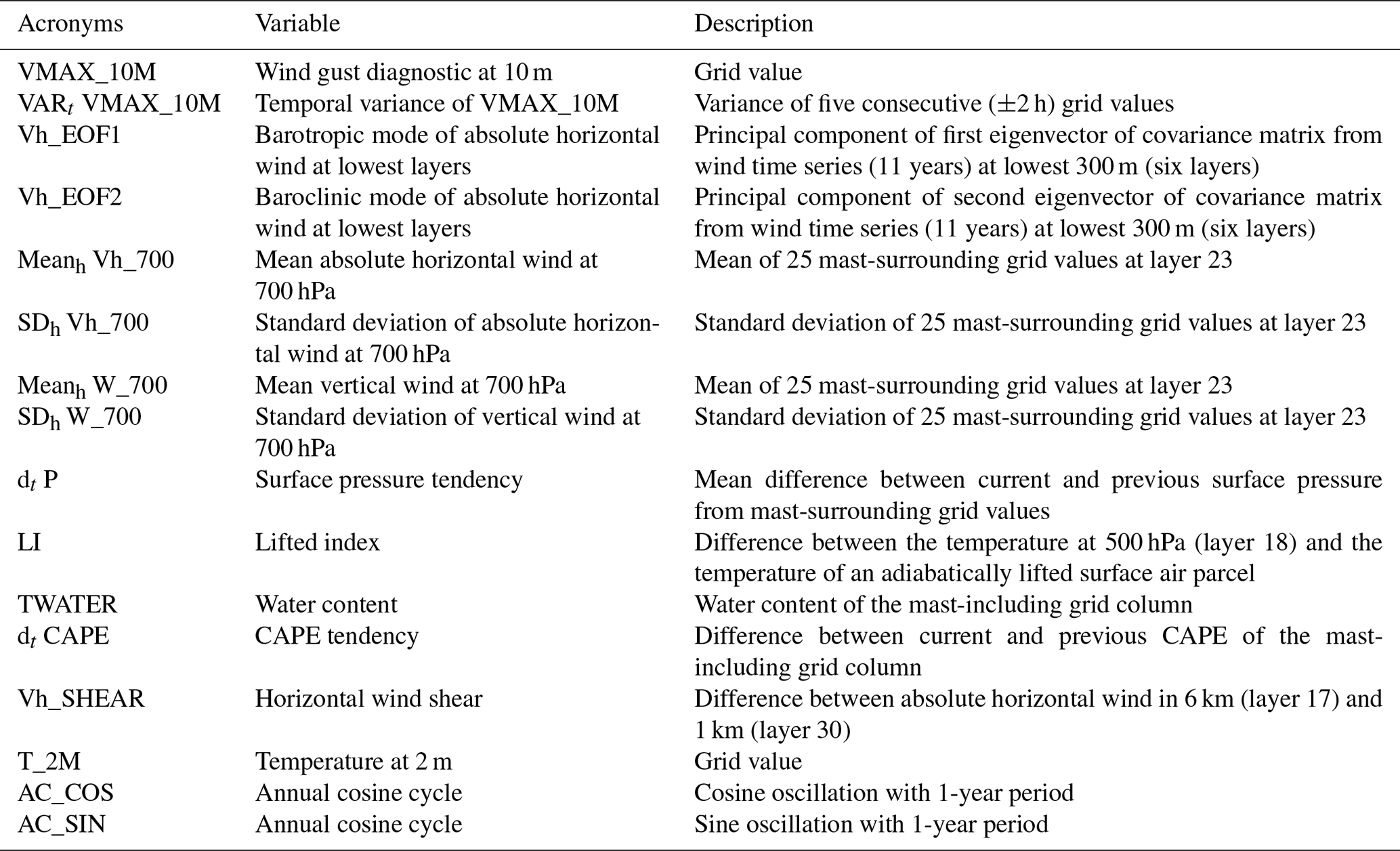
We consider the following variables as covariates: the wind gust diagnostic at 10 m (VMAX_10M), the vertical profile of the horizontal wind speed at mast levels, the horizontal (Vh_700) and vertical (W_700) wind speed at 700 hPa, surface pressure tendency (dt P), the lifted index (LI), total water content (TWATER), atmospheric temperature at a height of 2 m (T_2M), tendency in convective available potential energy (dt CAPE), vertical shear of horizontal wind between 6 and 1 km (Vh_SHEAR), the temporal variance of VMAX_10M (VARt VMAX_10M), and the phase of the annual cycle. For a summary of the covariates, see Table 1. All covariates are standardized before they enter the cGEV regression model.
Table 1List of preselected covariates from the COSMO-REA6 reanalysis.
The gust diagnostic in COSMO-REA6 is probably the most informative variable, as it aims as an estimate of the potential strength of a gust near the surface. On the one hand, gusts are generated by turbulent deflection of upper air wind to the surface (Brasseur, 2001) and, on the other hand, they are generated by convective downdraughts (Nakamura et al., 1996). The turbulent gust diagnostic in COSMO-REA6 is given by an empirical relation to the 10 m wind velocity and the surface drag coefficient for momentum (Schulz and Heise, 2003; Schulz, 2008). The convective gust diagnostic depends on the downdraught formulation in the convection scheme (Schulz and Heise, 2003) and includes the height and the kinetic energy of the downdraught. VMAX_10M is the maximum of the turbulent and convective gust diagnostic. The differences between the observed gusts at a height of 10 m at the Hamburg Weather Mast and the COSMO-REA6 gust diagnostics are displayed in Fig. 1. The differences have a negative bias of about −1.03 m s−1, i.e. COSMO-REA6 slightly overestimates the strength of the gusts. The standard deviation amounts to about 1.8 m s−1. We also include the variance of VMAX_10M over the period from 2 h before to 2 h after the respective analysis time (Vart VMAX_10M) as a covariate.
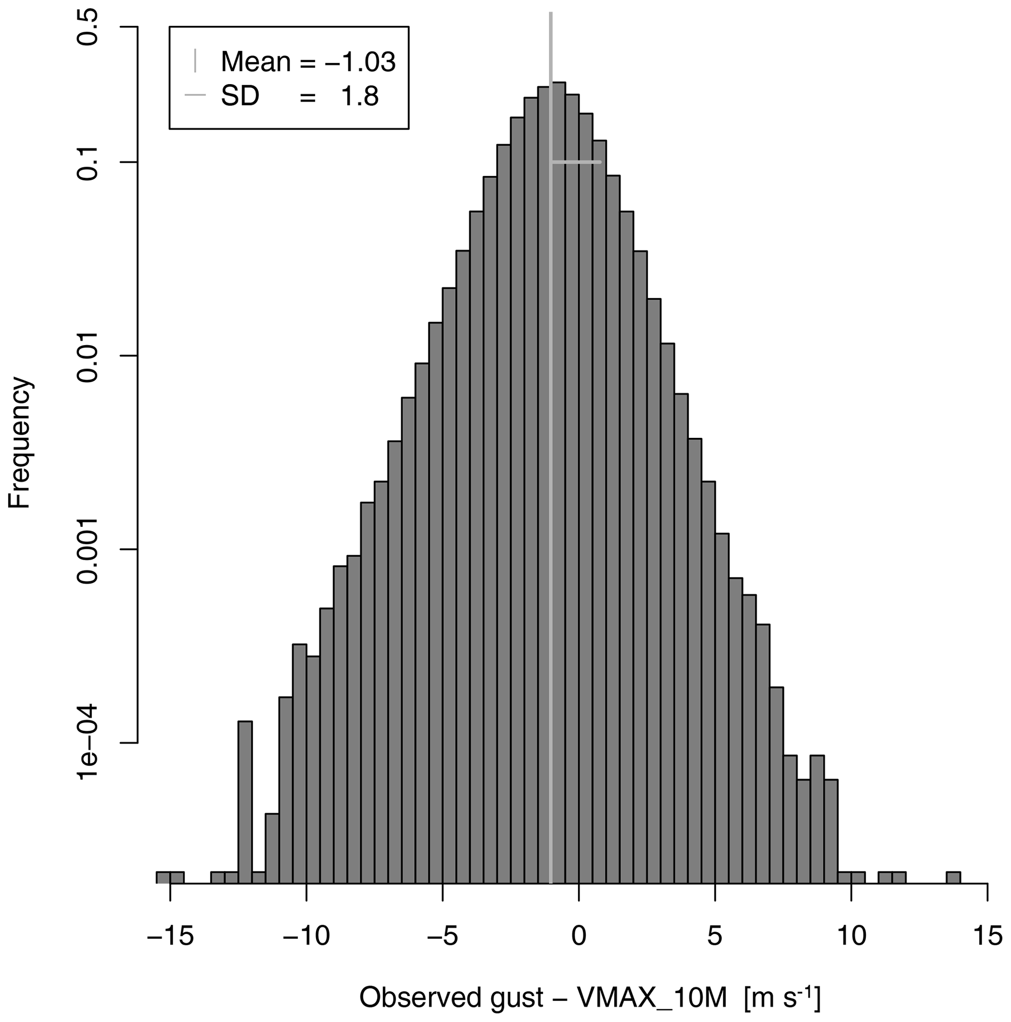
Figure 1Histogram of differences between observed gusts at 10 m and the COSMO-REA6 10 m gust diagnostic.
As gusts are naturally related to mean wind speed, we include the horizontal velocities at the station location. COSMO-REA6 has a staggered grid, so the wind velocity is given as the absolute velocity of the centred zonal and meridional velocities. To represent the state of the local vertical profile of the horizontal wind velocity in a height-independent variable, we use a principal component analysis. A principal component analysis of the wind velocity at the different heights reveals that most variability (about 92 %) is explained by a mode of variability where all wind anomalies have the same sign, with a slight increase in variability at higher levels. The second mode of variability, which explains about 6 % of the total variability, represents a dipole (i.e. baroclinic) structure with positive anomalies in the upper two levels and corresponding negative anomalies in the lowest three levels. The latter mode is called the baroclinic wind mode (Vh_EOF2), whereas the former – although not completely barotropic – is called the barotropic wind mode (Vh_EOF1).
An important index to capture vertical instability is the lifted index (LI, e.g. Bott, 2016). It is defined as the difference between the temperature at 500 hPa and the temperature of an air parcel that is adiabatically lifted up from the surface to 500 hPa. Negative values indicate a potentially unstable atmosphere, which could lead to convection and, hence, gusts. If convection takes place, CAPE is consumed and a tendency in CAPE is seen in the reanalysis data. Thus, we include the tendency of CAPE (dt CAPE) over 1 h as a covariate. We also use the total water content (TWATER) of the column that includes the location of the Hamburg Weather Mast. All of these covariates are calculated for the vertical column of the grid point closest to the mast location.
We further include information on the atmospheric circulation above the boundary layer at 700 hPa surrounding the Hamburg Weather Mast. The wind velocities at the closest 25 grid cells are used to calculate an averaged horizontal (Meanh Vh_700) and vertical (Meanh W_700) wind speed as well as the respective standard deviations over that region SDh Vh_700, and SDh W_700 respectively. Another possible indicator for gust activity is the tendency of pressure at the surface over 1 h within the area surrounding the weather mast. The pressure tendency dt P is again an averaged tendency over the 25 nearest grid points.
The annual cycle is represented by a linear combination of a sine and cosine function with a period of 1 year (AC_COS and AC_SIN).
Several decisions are needed before setting up the post-processing approach. The first concerns the threshold for censoring. We choose the 50 % quantile of the observations at each level respectively, which corresponds to 5.79 m s−1 (at a hight of 10 m), 7.40 m s−1 (at 50 m), 8.65 m s−1 (at 110 m), 9.69 m s−1 (at 175 m), and 10.54 m s−1 (at 250 m). We further decide to fix the shape parameter ξ to zero for the two abovementioned reasons. First, studies of wind gusts often reveal a negative ξ for the fitted GEV (e.g. Friederichs et al., 2009), i.e. a Weibull-type GEV with an upper end point. Any future gust above this end point would have predictive probability zero, which would results in a very bad forecast. Therefore, a Gumbel-type GEV reduced the risk of missing an extreme gust. The second reason is the stability of the maximum likelihood optimization. The estimation of ξ introduces large uncertainties. Particularly with a large number of parameters (i.e. covariates), the optimization procedures is often stuck in a local maximum. This is particularly critical, if the domain of the distribution is restricted, as is the case for a Weibull-type GEV. Finally, to approximate the vertical variation of the cGEV parameters we use the first three Legendre polynomials P0 (constant), P1 (linear), and P2 (quadratic). Higher-order polynomials did not provide any added value (not shown).
Table 2Estimates of the regression coefficients using the Legendre model with K=2. Estimates are derived without penalization including the selected covariates. Mean and standard deviation are derived from the 11 estimates using cross-validation. Bold text indicates the parameters that resisted the LASSO penalization. No value is given if the variable is not included in the Legendre model.
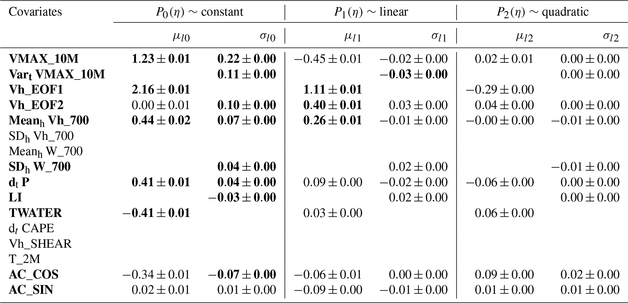
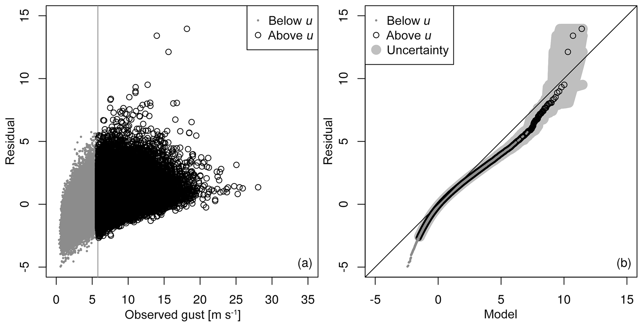
Figure 2Diagnostics for Legendre model without VARt VMAX_10M and with a threshold of u=5.79 m s−1 at 10 m: (a) scatter plot of the standard Gumbel residual against observed gusts, and (b) Q–Q plot of the residuals against the standard model. Uncertainty is given in light grey as the range of a 100-member bootstrap sample generated with blocks of 10 consecutive days.
4.1 Model selection
The next step is the selection of the most important predictors. The variable selection is performed using the LASSO approach including cross-validation, providing 11 sets of penalized regression coefficients. The value of λ is determined by analysing the cross-validated LASSO path, which describes the changes in the regression parameters with respect to λ. The LASSO approach is very sensitive to λ. We chose , where m is the number of observations, as a larger λ leads to an excessive penalization, whereas a smaller λ accepts almost all covariates as relevant. As the covariates are standardized, the absolute value of each related coefficient is proportional to the importance of the covariate. We select a covariate if at least one of its three Legendre coefficients is consistently below or above zero for all 11 cross-validation samples. If a covariate is selected, we allow for full flexibility in the vertical including all three Legendre polynomials, as the higher-order polynomials, in particular, are very sensitive to the penalization.
Table 2 represents the regression coefficients obtained for the Legendre model with the selected covariates but without penalization. The parameters that resisted the penalization are displayed using bold numbers. If no regression coefficient is given in Table 2, the covariate was not selected. For the location parameter μ, the most informative covariates are generally the barotropic wind mode (Vh_EOF1) and the gust diagnosis (VMAX_10M). The averaged horizontal wind (Meanh Vh_700) provides some additional information. The pressure tendency (dt P) is similarly important, with a positive pressure tendency (e.g. a passing cold front) being related to an increase in gust activity and TWATER with a negative regression coefficient.
The influence of the covariates on σ is generally weaker than on μ. Here, the most informative covariate is indeed VMAX_10M, leading to an increase in σ if VMAX_10M is large. The variance of the predictive cGEV is significantly increased if Vart VMAX_10M is large. We discuss the influence of Vart VMAX_10M later in this section. Vh_EOF1 was not selected by the LASSO approach, but some additional information is provided by the baroclinic wind mode (Vh_EOF2). The weak influence of AC_COS indicates a slight increase in gust activity during summer, which is not explained by the other covariates.
The interpretation of the role of the covariates is not straightforward, as the selected covariates are correlated. This is particularly the case for the 10 m gust diagnostic and the barotropic wind mode. Therefore, the omission of one would lead to a modified role of the other. The most important covariates, notably the wind covariates, roughly reveal that stronger winds results in increased μ and σ parameters of the cGEV. Further, there is a remarkable influence of integrated water content and the pressure tendency. A positive pressure tendency is associated with stronger wind gusts, and one may argue that the probability of gusts is increase during the passage of a cold front. The role of TWATER is less obvious at first. TWATER shows a pronounced annual cycle, as the warmer atmosphere during summer has a larger water vapour capacity. Likewise, gusts are stronger during winter than during summer on average. The mean 10 m wind gust at the Hamburg Weather Mast is about 6.3 m s−1 in winter and 5.78 m s−1 in summer. Thus, one should be careful interpreting this result, as the negative relation between TWATER and gustiness may only be a consequence of the annual cycle and should not be interpreted as a causal relation.
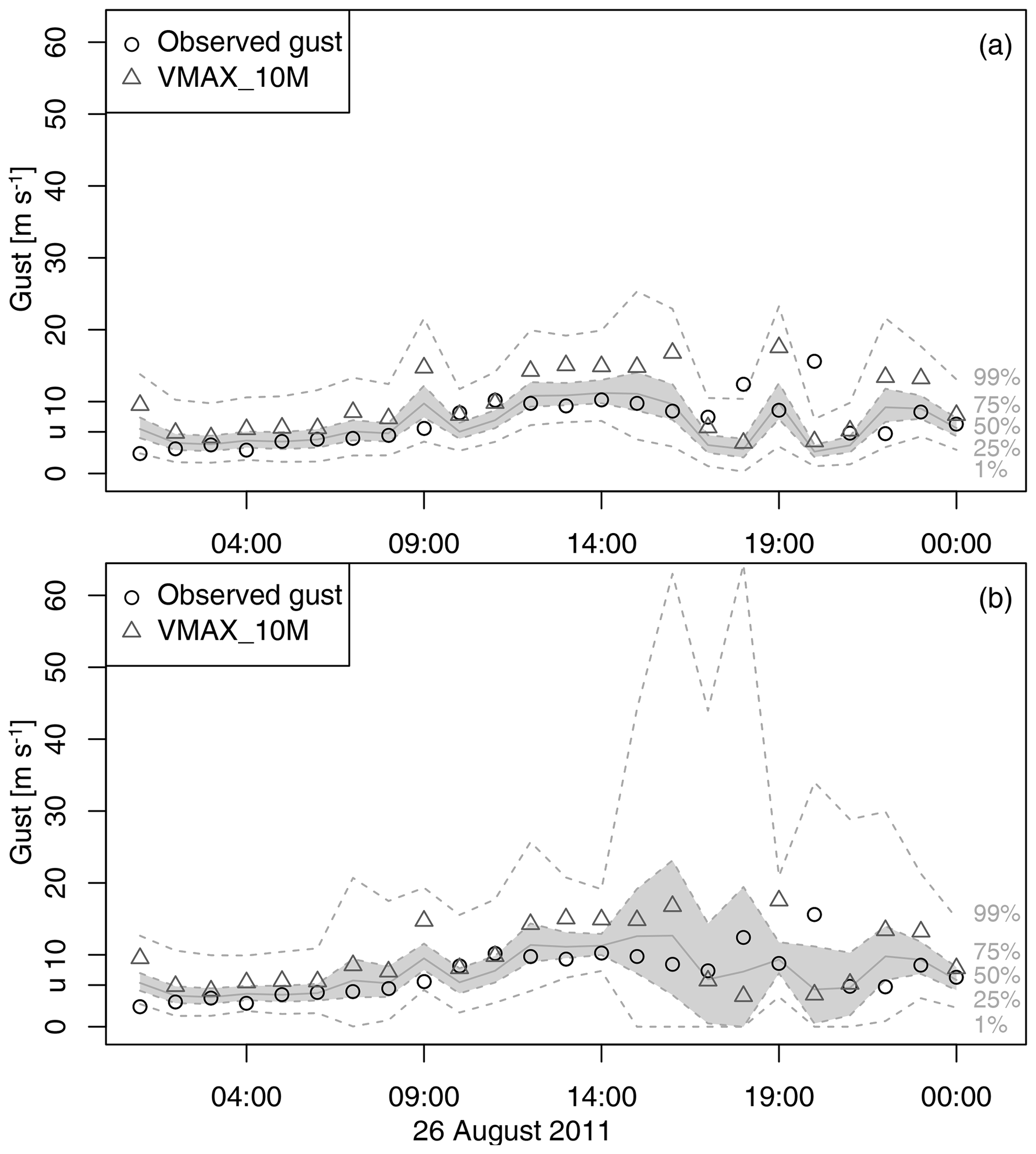
Figure 3Post-processing of gusts on 26 August 2011 at 10 m: (a) Legendre model without VARt VMAX_10M; (b) Legendre model. Shading indicates the predictive interquartile range, the grey line indicates the median, and dashed lines indicate the 1 % and 99 % quantiles respectively. The observed gust are shown as circles, and the 10 m gust diagnostic is shown as triangles.
The covariate Vart VMAX_10M was not included in an earlier version of the Legendre model. Figure 2a shows the residuals using the Legendre model without Vart VMAX_10M against the observed gusts. The highest gusts above 20 m s−1 are well captured, as the residuals are generally small with values between −1 and 4. However, the Q–Q plot in Fig. 2b indicates three outliers that are not well captured by the model. The outliers correspond to gusts of about 15 to 20 m s−1 and are therefore of relevance. Two of the outliers occur on 26 August 2011. Figure 3a shows the model predictions on 26 August 2011. The predictive quantiles are calculated using a GEV with the Legendre estimates of the cGEV. The outliers are observed at 18:00 and 20:00 CET respectively and well exceed the predictive 99 % quantiles, whereas COSMO-REA6 diagnoses a gust of about 20 m s−1 at 19:00 CET. The observed gusts are related to two convective storms that passed over Hamburg. The COSMO-REA6 analysed a convective cell over Hamburg but with incorrect timing. The adjusted prediction including VARt VMAX_10M is shown in Fig. 3b. We now see an increase in the predicted range of the gusts such that the observed gusts are within the 99 % range of the prediction. The Q–Q plot of the Legendre model including VARt VMAX_10M (Fig. 4a) shows that the two outliers on 26 August 2011 are now eliminated; however, this occurs at the cost that the Legendre model now slightly overestimates the high quantiles. With the inclusion of the temporal variability of the 10 m gust diagnostic, we improved the post-processing model mainly by increasing the σ parameter when gustiness in the reanalysis strongly varies over time. Thus, the role of this covariate is to account for timing errors in the reanalysis, which might be particularly large for weather situations that favour small convective cells. This method successfully eliminates two of the three outliers. Figure 4b shows the Q–Q plot at 110 m. The remaining outlier is also present at a higher level, but the overestimation of the high quantiles is much weaker than at 10 m.
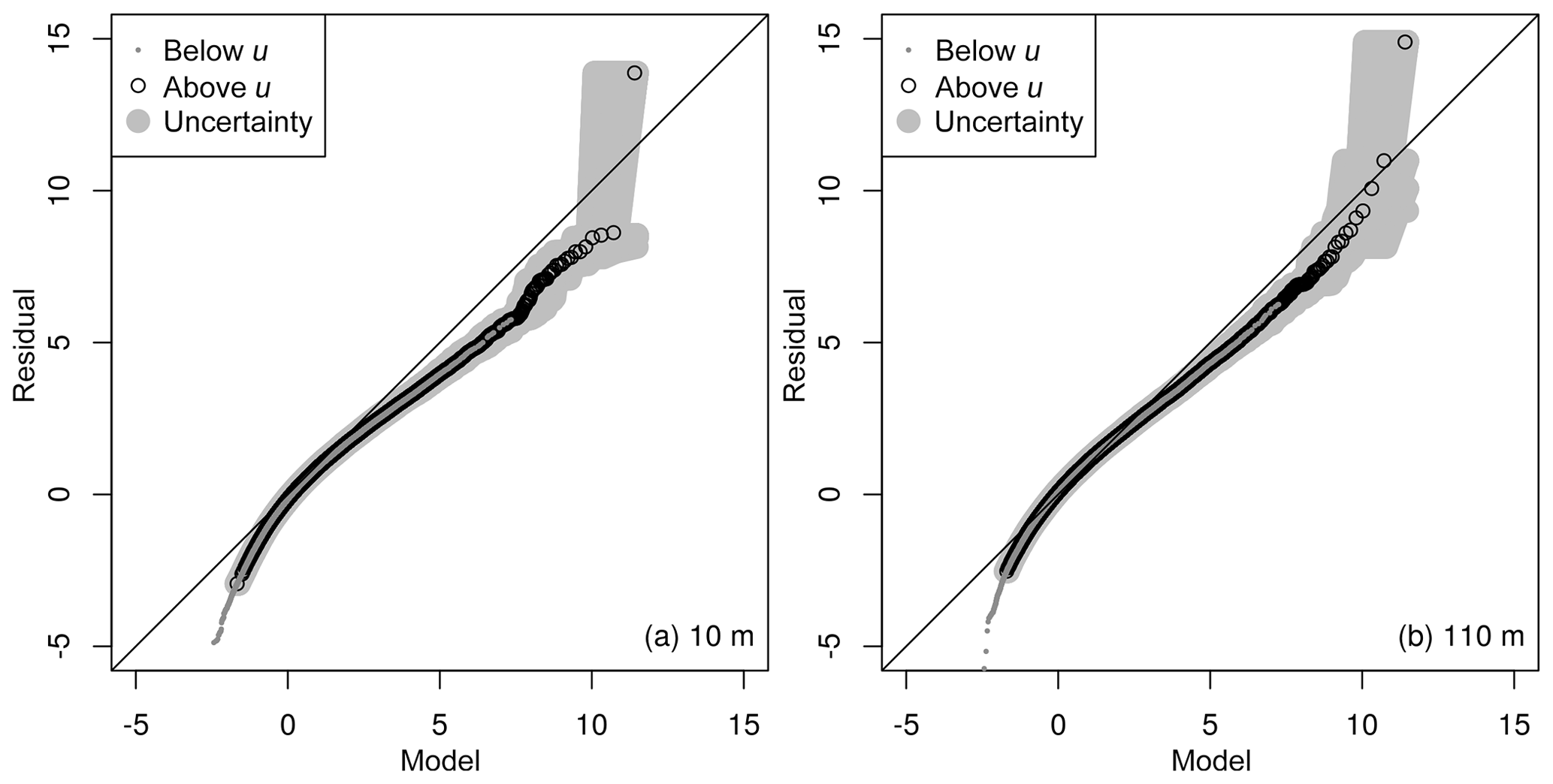
Figure 4Q–Q plots for the Legendre model (a) at 10 m and (b) at 110 m with bootstrap uncertainty, as in Fig. 2.

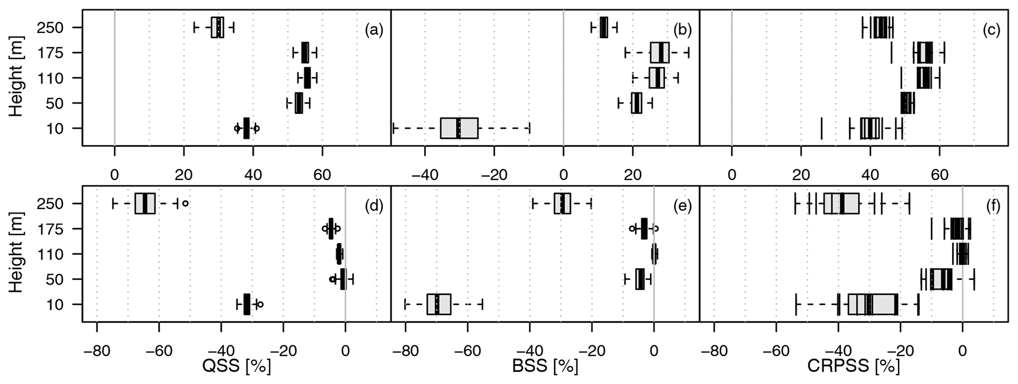
Figure 5Verification skill scores for the Legendre model against climatology (a–c) and against the layer-wise model (d–f). The QSS is given for the predictive τ=99 % quantile in (a) and (d); the BSS for thresholds corresponding to the observations' 99 % quantile (u=14.8 m s−1 at 10 m, u=19.26 m s−1 at 50 m, u=21.01 m s−1 at 110 m, u=22.55 m s−1 at 175 m, and u=23.97 m s−1 at 250 m) in (b) and (e); and the CRPSS in (c) and (f). For QSS and BSS, the box and whiskers represent the 100-member bootstrap sample, with the box giving the interquartile range. The range of the whiskers is a maximum of 1.5 times the width of the box. For the CRPSS, the boxes represent the 11 cross-validated estimates.
4.2 Verification
The post-processing method is assessed using proper verification skill scores. We first assess the effect of the Legendre approximation. Figure 5a–c show skill scores of the layer-wise model with climatology as a reference. The 99 % QSS indicates remarkable improvements of about 45 % to 60 % with respect to climatology. The BSS evaluates the predictive probability of exceeding a threshold defined as the 99 % quantile of the observations at each level respectively. The respective thresholds are given in the caption of Fig. 5. The BSS is smaller than the QSS with values ranging from about 10 % in the lowest level to 40 % at 250 m. The CRPSS ranges between 40 % and 50 %. Ideally, an approximation of the vertical variation of the cGEV parameters by Legendre polynomials should not decrease the skill scores. Figure 5d–f show the skill score of the Legendre model with the layer-wise model as reference. The reduction in skill is not larger than 7 % and is largest in the QSS and BSS at the 10 m level. We conclude that the Legendre model represents an appropriate model for all layers.
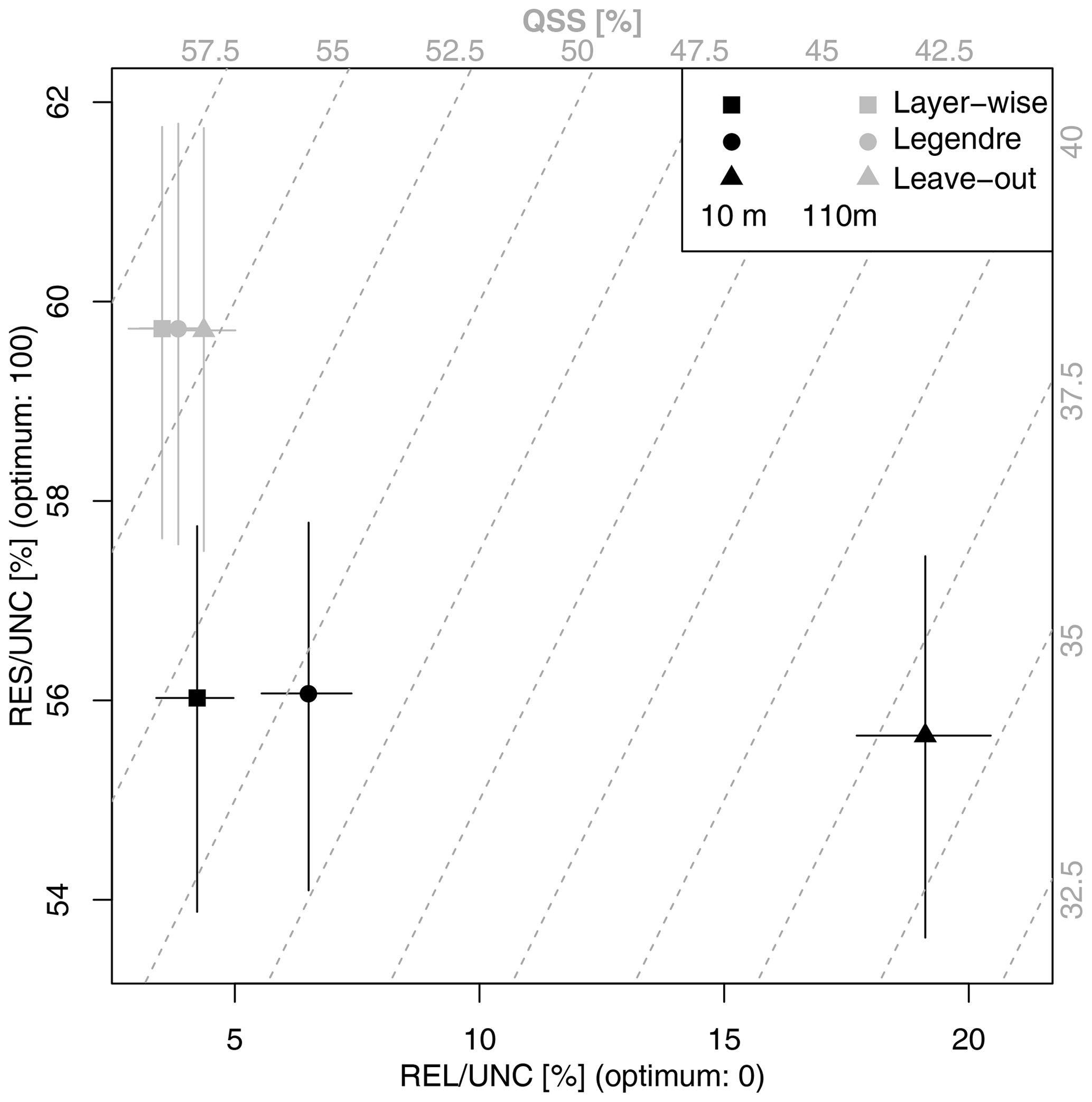
Figure 7Decomposition of the QSS of the predictive 99 % quantile at 10 m (black) and 110 m (grey) into scaled resolution (RES/UNC) and scaled reliability (REL/UNC) for the layer-wise, Legendre, and leave-out models. The crosses show the range of the 100-member bootstrap samples. The grey dashed lines indicate the QSS. The QSS amount is given on the upper and the right axes (grey numbers).
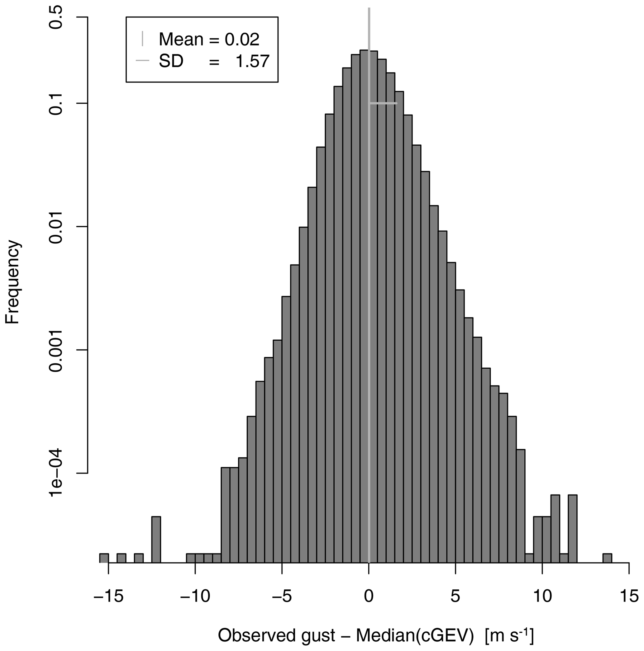
Figure 8Histogram of differences between observed gusts at 10 m and the GEV median prediction at 10 m.
The advantage of the Legendre model is the possibility to provide predictions at levels where no observations are available. Figure 6a–c represent the skill score for the leave-out model with climatology as a reference. All skill scores show a strong decrease in skill at 10 and 250 m. At 10 m, the BSS even shows negative skill. In Fig. 6d–f, the direct comparisons show that, except for at the lowest and highest level, the loss in skill is only of about 10 % at the most when compared to what is obtained with the layer-wise model. The decomposition of the QSS of the 99 % quantiles at 10 and 110 m shows that the loss in predictive skill is mainly due to the reliability term, while the resolution remains almost constant; it also shows that the reliability is particularly bad for the leave-out model at a height of 10 m. Thus, the interpolation of the cGEV parameters is applicable, whereas an extrapolation to the 10 and the 250 m levels fails to provide a reliable predictive distribution.
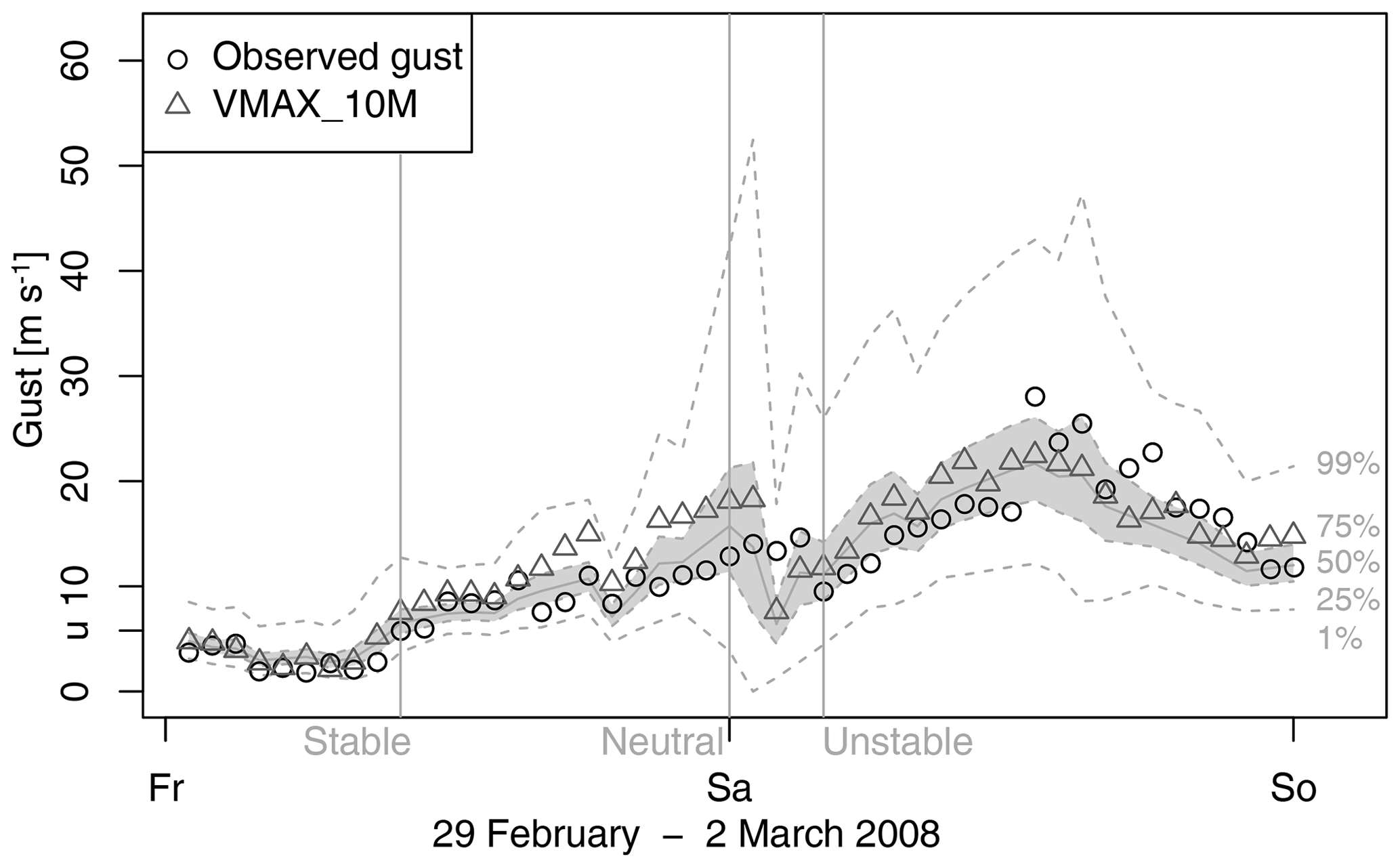
Figure 9Post-processing of gusts on 29 February and 1 March 2008 at 10 m. Shading indicates the predictive interquartile range, the grey line indicates the median, and dashed lines indicate the 1 % and 99 % quantiles respectively. The observed gust are shown as circles, and the 10 m gust diagnostic is shown as triangles. The vertical lines indicate times with stable (LI of 8.7 K), neutral (LI of 2.4 K), and unstable (LI of −3.1 K) conditions.
The post-processing method aims at an improved 10 m wind gust diagnostic. In order to compare the post-processed gust distribution with the COSMO-REA6 gust diagnostic, we calculate the median of a GEV using the cGEV parameters of the layer-wise model. Figure 8 shows the histogram of differences between the observations and the mean at 10 m. Compared with the gust diagnostic of COSMO-REA6 in Fig. 1, we see an improvement as the bias almost vanishes and the standard deviation of the differences is reduced to 1.57 m s−1. Large differences still occur in situations where the reanalysis is not able to simulate small-scale convective cells correctly in terms of timing or location.
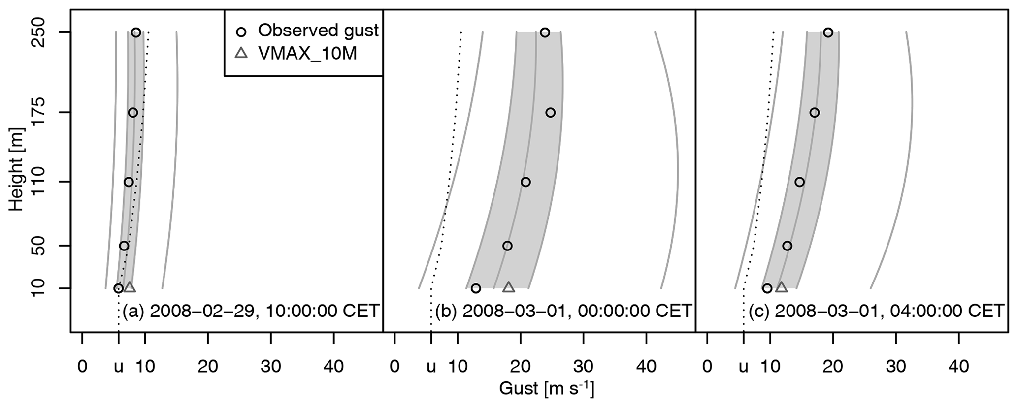
Figure 10Vertical post-processing of gusts using the Legendre model for times highlighted in Fig. 9. The grey solid lines indicate the conditional quantiles using a GEV at probabilities 1 %, 25 %, 50 %, 75 %, and 99 %. The dotted line represents the censoring threshold.
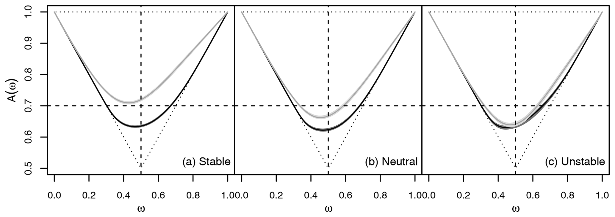
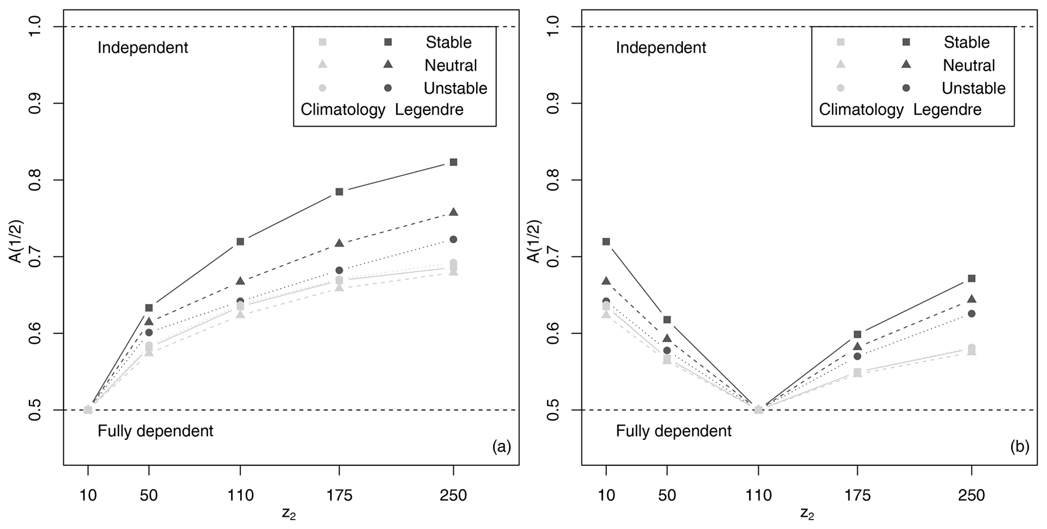
Figure 11Pickands dependence function of 10 and 110 m for the Legendre model (light grey) and climatology (dark grey). According the LI, the data are classified into 53 % stable (a), 36 % neutral (b), and 11 % unstable (c) cases. Uncertainty is derived using block bootstrapping. A horizontal line at 0.7 is displayed for visualization purpose only. The dotted lines indicate complete independence with A(ω)=1 as well as complete dependence.
4.3 Application and bivariate dependency
To illustrate the post-processing using the Legendre model, we have a closer look at storm Emma between 29 February and 1 March 2008. During Emma, we observe the largest gusts at 10 m over the whole observation period of the Hamburg Weather Mast, with 28.07 m s−1 on 1 March 2008 between 12:00 and 13:00 CET. The storm hit a large region in Europe. In Hamburg, a storm surge also flushed parts of the city. COSMO-REA6 has difficulties precisely capturing the evolution of the storm over Hamburg (Fig. 9). As in the reanalysis, the post-processing approach misses the highest gusts on Saturday, 1 March 2008, although the prediction is provided with reasonably high uncertainties. A better prediction is generated by the post-processing method on Friday, 28 February 2008. By way of example, we selected 3 h that represent differently stratified atmosphere, as indicated by vertical lines in Fig. 9. According to Bott (2016), we characterize the atmosphere as stable if LI ≥ 6 K, as neutral if 6 K ≥ LI ≥ −2 K, and as unstable if −2 K ≥ LI. Figure 10 shows the corresponding vertical profiles of the predictive GEV distribution. In all cases, the median prediction is in good agreement with the observations. On 29 February 2008 at 10:00 CET (stable atmosphere), the observed gusts are within the interquartile range of the predictive GEV and slightly below the censoring threshold. The variance of the predictive GEV is small. On 1 March 2008 at 01:00 CET (neutral atmosphere), the interquartile range is larger, and the vertical variation of the gusts is also larger and well captured by the predictive GEV. On 1 March 2008 at 04:00 CET, the atmosphere is highly unstable. The observed gust are very close to the median of the predictive GEV. Note that the LI only influences the cGEV scale parameter and that the regression coefficient is small (see Table 2).
Figure 10 suggests that the gusts do not vary independently of each other. In order to investigate the height dependency, we calculate the bivariate Pickands dependency function following Eq. (10). Transformation to standard Fréchet is performed using the parameters for the climatological cGEV (i.e. assuming a homogeneous marginal cGEV independently at each height) and from the Legendre model (i.e. accounting for non-homogeneity by post-processing). Figure 11 shows the estimated Pickands dependence function between the gust residuals at 10 and 110 m respectively for the stable, neutral, and unstable cases. Using homogeneous marginals, the dependence between the gusts at the two levels is strong and seems independent of the stability of the atmosphere. Post-processing strongly reduces vertical dependencies in the residuals. The weakest dependence is observed in a stable atmosphere, whereas dependence for the post-processed residuals is almost as strong as for the climatological residuals in an unstable atmosphere. Variation in the dependency structure is reasonable, as the more unstable the atmosphere, the more vertical mixing is induced.
The dependence between residual gusts at 10 m and higher levels decreased with distance in the vertical, as indicated by the value of the Pickands dependency function at in Fig. 12a. Again, for the climatological residuals, dependence is strong and decreases less with distance compared with the post-processed residuals. The decrease in dependence with distance is largest during cases with a stable atmosphere. A simple relation between the strength of the dependency and the distance between layers is not given, as e.g. the dependence between gusts at 110 and 250 m is stronger than between gusts at 110 and 10 m (Fig. 12b).
This study presents a post-processing approach for hourly wind gusts at different vertical heights from observations at the Hamburg Weather Mast. The post-processing model is based on a conditional censored Gumbel-type GEV distribution. The censoring threshold is defined as the 50 % quantile of the observations at each mast level respectively. The censoring approach performs well and leads to a good representation of the larger gusts.
A LASSO approach is used to select the most informative covariates. The selected variables are the COSMO-REA6 wind gust diagnostic at 10 m and its temporal variance, the barotropic and baroclinic mode of absolute horizontal wind speed, the mean absolute horizontal wind at 700 hPa, the pressure tendency, the lifted index, and the grid column water content. The predictive cGEV median provides an improved gust estimate compared with the reanalysis gust diagnostic at 10 m.
Vertical variations of the cGEV parameters are approximated using the three lowest-order Legendre polynomials. Although the best scores are obtained if the post-processing is performed for each level independently, the unified description only results in a slight degradation of skill at the intermediate layers. The unified description induces a small bias at 10 m, with gusts being slightly overestimated. Extrapolation of the cGEV parameters towards the 10 m level and the uppermost level generates large biases and thereby degrades skill. In contrast, interpolation towards intermediate levels is very successful, as the degradation in terms of predictive skill is barely significant when excluding the model level. Therefore, the post-processing method not only provides calibrated predictive distributions of gusts at the observed levels but also at arbitrary heights of the weather mast.
Our post-processing strategy is applicable to NWP forecasts without relevant changes, except for the selection of the covariates. Particularly, if applied to ensemble forecasts, additional predictors such as the predictive uncertainty, quantiles, or probabilities for threshold exceedances as derived from the ensemble may be considered. For an example of how to include ensemble statistics into the post-processing approach, see Wahl (2015). In Friederichs et al. (2018), a similar approach is applied to COSMO-DE-EPS forecasts to predict 6-hourly maxima of 10 m wind gusts. Although not really comparable, i.e. hourly maxima in this study but 6-hourly maxima in the above-mentioned study and a variety of covariates as predictors in this study but wind variables only in Friederichs et al. (2018), they obtain a BSS for a 14.8 m s−1 threshold and a QSS for the 99 % quantile of about 40 %. The forecast lead time in their study is between 12 and 18 h. This suggests that forecast errors at lead times of about 1 d for 6-hourly maxima are small enough to obtain reasonable skill. The respective skill scores at the 10 m level in this study amount to about 24 % for the BSS and about 53 % for the QSS. The skill scores are comparable and suggest that similar skill scores may be obtained at higher levels.
The strength of the spatial dependency of gusts is assessed using the Pickands dependence function. The gusts at the different heights are highly dependent. Conditioning the gusts on the COSMO-REA6 covariates reduces the dependency of the residuals between heights. This reduction in dependence is significantly modulated by the stability of the atmosphere as given by the lifted index in the sense that an unstable atmosphere increases mixing and, therefore, dependency. Dependency is not simply a function of distance. For a full spatial model description of the gusts, dependency needs to be modelled as a function of atmospheric condition as well as height.
The post-processing model as estimated for the Hamburg Weather Mast should, in principle, be transferable to other locations. This may be tested using observations from other weather masts in the model region. However, difficulties may arise because observations from different masts might be processed differently or made with different instruments. Furthermore, different topography or other local parameters could introduce systematic biases. Moreover, at other locations, only measurements of the 10 m are available; however it would be of interest to assess how well gust statistics that are only based on observations at 10 m would be estimated at higher levels. The ultimate goal of this work would be to provide estimates of vertical gust statistics at any location in the COSMO-REA6 reanalysis domain.
The wind gust observations from the Hamburg Weather Mast were provided by Ingo Lange from the Meteorological Institute of the University of Hamburg (further information and contact: https://wettermast.uni-hamburg.de, last access: 20 April 2020). The COSMO-REA6 data are stored at the DWD and are accessible via ftp://opendata.dwd.de/climate_environment/REA/ (last access: 20 April 2020). For further information, see https://www.dwd.de/DE/klimaumwelt/klimaueberwachung/reanalyse/reanalyse_node.html (last access: 20 April 2020).
JS and PF jointly developed the concept and methodology for this work. JS carried out the post-processing and the visualization of the results, and PF supervised the process. JS was the lead author on the paper with input from PF.
The authors declare that they have no conflict of interest.
This article is part of the special issue “Advances in post-processing and blending of deterministic and ensemble forecasts”. It is not associated with a conference.
We are grateful to Ingo Lange and the Meteorological Institute at the University of Hamburg for the provision of the wind data from the Hamburg Weather Mast. Special thanks go to Sebastian Buschow for helpful discussions and valuable ideas. We wish to thank Stéphane Vannitsem and the two anonymous reviewers for their constructive comments.
This work has been conducted in the framework of the Hans Ertel Centre for Weather Research funded by the German Federal Ministry for Transportation and Digital Infrastructure (grant no. BMVI/DWD 4818DWDP5A).
This paper was edited by Stéphane Vannitsem and reviewed by two anonymous referees.
Baldauf, M., Seifert, A., Förstner, J., Majewski, D., Raschendorfer, M., and Reinhardt, T.: Operational Convective-Scale Numerical Weather Prediction with the COSMO Model: Description and Sensitivities, Mon. Weather Rev., 139, 3887–3905, https://doi.org/10.1175/MWR-D-10-05013.1, 2011. a
Baran, S. and Lerch, S.: Log-normal distribution based Ensemble Model Output Statistics models for probabilistic wind-speed forecasting, Q. J. Roy. Meteor. Soc., 141, 2289–2299, https://doi.org/10.1002/qj.2521, 2015. a
Bentzien, S. and Friederichs, P.: Decomposition and graphical portrayal of the quantile score, Q. J. Roy. Meteor. Soc., 140, 1924–1934, https://doi.org/10.1002/qj.2284, 2014. a, b
Bollmeyer, C., Keller, J. D., Ohlwein, C., Wahl, S., Crewell, S., Friederichs, P., Hense, A., Keune, J., Kneifel, S., Pscheidt, I., Redl, S., and Steinke, S.: Towards a high-resolution regional reanalysis for the European CORDEX domain, Q. J. Roy. Meteor. Soc., 141, 1–15, https://doi.org/10.1002/qj.2486, 2014. a, b, c
Born, K., Ludwig, P., and Pinto, J. G.: Wind gust estimation for Mid-European winter storms: towards a probabilistic view, Tellus A, 64, 17471, https://doi.org/10.3402/tellusa.v64i0.17471, 2012. a
Bott, A.: Synoptische Meteorologie, Springer Spektrum, 2016. a, b
Brasseur, O.: Development and Application of a Physical Approach to Estimating Wind Gusts, Mon. Weather Rev., 129, 5–25, https://doi.org/10.1175/1520-0493(2001)129<0005:daaoap>2.0.co;2, 2001. a
Brier, G. W.: The Statistical Theory of Turbulence and the Problem of Diffusion in the Atmosphere, J. Meteorol., 7, 283–290, https://doi.org/10.1175/1520-0469(1950)007<0283:tstota>2.0.co;2, 1950. a
Brümmer, B., Lange, I., and Konow, H.: Atmospheric boundary layer measurements at the 280 m high Hamburg weather mast 1995-2011: mean annual and diurnal cycles, Meteorol. Z., 21, 319–335, https://doi.org/10.1127/0941-2948/2012/0338, 2012. a, b
Doms, G. and Baldauf, M.: A description of the non-hydrostatic regional model LM – Part I: Dynamics and numerics, Tech. rep., Deutscher Wetterdienst, Offenbach, Germany, available at: http://www.cosmo-model.org/content/model/documentation/core/cosmoDyncsNumcs.pdf (last access: 17 April 2020), 2011. a
Doms, G., Förster, J., Heise, E., Herzog, H. J., Mironov, D., Raschendorfer, M., Reinhardt, T., Ritter, B., Schrodin, R., and Vogel, J. P. S. G.: A description of the non-hydrostatic regional model LM – Part II: Physical Parameterization, Tech. rep., Deutscher Wetterdienst, Offenbach, Germany, available at: http://www.cosmo-model.org/content/model/documentation/core/cosmoPhysParamtr.pdf (last access: 17 April 2020), 2011. a
Fisher, R. A. and Tippett, L. H.: On the estimation of the frequency distributions of the largest or smallest member of a sample, Math. Proc. Cambridge, 24, 180–190, 1928. a
Frank, C. W., Pospichal, B., Wahl, S., Keller, J. D., Hense, A., and Crewell, S.: The added value of high resolution regional reanalyses for wind power applications, Renew. Energ., 148, 1094–1109, https://doi.org/10.1016/j.renene.2019.09.138, 2019. a
Friederichs, P.: Statistical downscaling of extreme precipitation events using extreme value theory, Extremes, 13, 109–132, https://doi.org/10.1007/s10687-010-0107-5, 2010. a
Friederichs, P. and Hense, A.: Statistical Downscaling of Extreme Precipitation Events Using Censored Quantile Regression, Mon. Weather Rev., 135, 2365–2378, https://doi.org/10.1175/MWR3403.1, 2007. a
Friederichs, P. and Thorarinsdottir, T. L.: Forecast verification for extreme value distributions with an application to probabilistic peak wind prediction, Environmetrics, 23, 579–594, https://doi.org/10.1002/env.2176, 2012. a
Friederichs, P., Göber, M., Bentzien, S., Lenz, A., and Krampitz, R.: A probabilistic analysis of wind gusts using extreme value statistics, Meteorol. Z., 18, 615–629, https://doi.org/10.1127/0941-2948/2009/0413, 2009. a, b
Friederichs, P., Wahl, S., and Buschow, S.: Postprocessing for Extreme Events, in: Statistical Postprocessing of Ensemble Forecasts, Elsevier, 127–154, https://doi.org/10.1016/b978-0-12-812372-0.00005-4, 2018. a, b, c, d
Gnedenko, B.: Sur La Distribution Limite Du Terme Maximum D'Une Serie Aleatoire, Ann. Math., 44, 423, https://doi.org/10.2307/1968974, 1943. a
Gneiting, T. and Raftery, A. E.: Strictly Proper Scoring Rules, Prediction, and Estimation, J. Am. Stat. Assoc., 102, 359–378, https://doi.org/10.1198/016214506000001437, 2007. a, b
Hall, P. and Tajvidi, N.: Distribution and Dependence-Function Estimation for Bivariate Extreme-Value Distributions, Bernoulli, 6, 835–844, https://doi.org/10.2307/3318758, 2000. a
Heffernan, J. E. and Stephenson, A. G.: ismev: An Introduction to Statistical Modeling of Extreme Values, available at: http://ral.ucar.edu/~ericg/softextreme.php (last access: 17 April 2020), 2016. a
Hersbach, H.: Decomposition of the Continuous Ranked Probability Score for Ensemble Prediction Systems, Weather Forecast., 15, 559–570, https://doi.org/10.1175/1520-0434(2000)015<0559:dotcrp>2.0.co;2, 2000. a, b
Lerch, S. and Thorarinsdottir, T. L.: Comparison of non-homogeneous regression models for probabilistic wind speed forecasting, Tellus A, 65, 21206, https://doi.org/10.3402/tellusa.v65i0.21206, 2013. a
Messner, J. W. and Pinson, P.: Online adaptive lasso estimation in vector autoregressive models for high dimensional wind power forecasting, Int. J. Forecasting, 35, 1485–1498, https://doi.org/10.1016/j.ijforecast.2018.02.001, 2019. a
Nakamura, K., Kershaw, R., and Gait, N.: Prediction of near-surface gusts generated by deep convection, Meteorol. Appl., 3, 157–167, https://doi.org/10.1002/met.5060030206, 1996. a
NCAR – Research Applications Laboratory: verification: Weather Forecast Verification Utilities, available at: https://cran.r-project.org/web/packages/verification/verification.pdf (last access: 17 April 2020), 2015. a
Oesting, M., Schlather, M., and Friederichs, P.: Statistical post-processing of forecasts for extremes using bivariate Brown-Resnick processes with an application to wind gusts, Extremes, 20, 309–332, https://doi.org/10.1007/s10687-016-0277-x, 2017. a
Pantillon, F., Lerch, S., Knippertz, P., and Corsmeier, U.: Forecasting wind gusts in winter storms using a calibrated convection-permitting ensemble, Q. J. Roy. Meteorol. Soc., 144, 1864–1881, https://doi.org/10.1002/qj.3380, 2018. a
Patlakas, P., Drakaki, E., Galanis, G., Spyrou, C., and Kallos, G.: Wind gust estimation by combining a numerical weather prediction model and statistical post-processing, Enrgy. Proced., 125, 190–198, https://doi.org/10.1016/j.egypro.2017.08.179, 2017. a
Petroliagis, T. I. and Pinson, P.: Early warnings of extreme winds using the ECMWF Extreme Forecast Index, Meteorol. Appl., 21, 171–185, https://doi.org/10.1002/met.1339, 2012. a
Pickands, J.: Multivariate extreme value distributions, Bull. Inst. Internat. Statist, 49, 859–878, 894–902, 1981. a, b
R Core Team: R: A Language and Environment for Statistical Computing, R Foundation for Statistical Computing, Vienna, Austria, available at: http://R-project.org/ (last access: 17 April 2020), 2016. a
Scheuerer, M.: Probabilistic quantitative precipitation forecasting using Ensemble Model Output Statistics, Q. J. Roy. Meteor. Soc., 140, 1086–1096, https://doi.org/10.1002/qj.2183, 2013. a
Scheuerer, M. and Möller, D.: Probabilistic wind speed forecasting on a grid based on ensemble model output statistics, Ann. Appl. Stat., 9, 1328–1349, https://doi.org/10.1214/15-AOAS843, 2015. a
Schulz, J.-P.: Revision of the Turbulent Gust Diagnostics in the COSMO Model, COSMO Newletter, 8, 17–22, available at: http://cosmo-model.org/content/model/documentation/newsLetters/newsLetter08/cnl8_schulz.pdf (last access: 17 April 2020), 2008. a
Schulz, J.-P. and Heise, E.: A New Scheme for Diagnosing Near-Surface Convective Gusts, COSMO Newletter, 3, 221–225, available at: http://cosmo-model.org/content/model/documentation/newsLetters/newsLetter03/cnl3-chp9-15.pdf (last access: 17 April 2020), 2003. a, b
Staid, A., Pinson, P., and Guikema, S. D.: Probabilistic maximum-value wind prediction for offshore environments, Wind Energy, 18, 1725–1738, https://doi.org/10.1002/we.1787, 2015. a
Stephenson, A.: evd: Functions for Extreme Value Distributions, available at: https://cran.r-project.org/web/packages/evd/evd.pdf (last access: 17 April 2020), 2018. a
Thorarinsdottir, T. L. and Johnson, M. S.: Probabilistic Wind Gust Forecasting Using Nonhomogeneous Gaussian Regression, Mon. Weather Rev., 140, 889–897, https://doi.org/10.1175/MWR-D-11-00075.1, 2012. a
Tibshirani, R.: Regression Shrinkage and Selection Via the Lasso, J. R. Stat. Soc. Ser. B Methodol., 58, 267–288, https://doi.org/10.1111/j.2517-6161.1996.tb02080.x, 1996. a, b
Wahl, S.: Uncertainty in mesoscale numerical weather prediction: probabilistic forecasting of precipitation, Dissertation, Rheinischen Friedrich-Wilhelms-Universität Bonn, 2015. a
World Meteorological Organization: Measurement of surface wind, Guide to Meteorological Instruments and Methods of Observation, 8, 196–213, available at: https://library.wmo.int/index.php?lvl=notice_display&id=12407 (last access: 20 April 2020), 2018. a
https://www.dwd.de/DE/klimaumwelt/klimaueberwachung/reanalyse/reanalyse_node.html (last access: 17 April 2020)