On fluctuating momentum exchange in idealised models of air–sea interaction

The dynamics of three local models, for momentum transfer at the air–sea interface, is compared. The models differ by whether or not the ocean velocity is included in the shear calculation applied to the ocean and the atmosphere. All three cases are employed in climate or ocean simulations. Analytic calculations for the models with deterministic and random forcing (white and coloured) are presented. The short-term behaviour is similar in all models, with only small quantitative differences, while the long-term behaviour differs qualitatively between the models. The fluctuation–dissipation relation, which connects the fast atmospheric motion to the slow oceanic dynamics, is established for all models with random forcing. The fluctuation–dissipation theorem, which compares the response to an external forcing to internal fluctuations, is established for a white-noise forcing and a coloured forcing when the phase space is augmented by the forcing variable. Using results from numerical integrations of stochastic differential equations, we show that the fluctuation theorem, which compares the probability of positive to negative fluxes of the same magnitude, averaged over time intervals of varying lengths, holds for the energy gained by the ocean from the atmosphere.

1 Introduction

The exchange of momentum, heat, water and chemical fluxes at the atmosphere–ocean interface is key to understanding the dynamics of the atmosphere, the ocean and the climate, as well as their response to changes in the forcing of the climate system (Stocker et al., 2013; Csanady, 2001). The fluxes at the interface are a result of a variety of physical processes over a large range of scales in space, from the molecular scale of spray dynamics (Veron, 2015), the scale of wave breaking (Melville, 1996), the sub-meso scale of fronts (Small et al., 2008), the synoptic scale of cyclones (Emanuel, 1986), the basin scale (Bjerknes, 1964) to the global scale (Alexander et al., 2002), and time, which interact in a non-linear way. The impact of the exchange on the atmosphere and ocean dynamics is usually described by local models, called bulk formulas (Kondo, 1975; Fairall et al., 1996; Castellari et al., 1998). They imitate the action of the non-explicitly resolved dynamics on the explicitly resolved dynamics in models and simulations of the atmosphere, ocean and climate dynamics.

In the present paper the exchange of momentum only is considered. It is caused by shear which depends on the atmospheric wind and many other physical quantities, such as the ocean velocity, the sea state and the density stratification in the atmosphere and the ocean. In this work three different approaches for parameterising the shear at the air–sea interface, which are all used in numerical simulations of atmosphere, ocean and climate dynamics, are compared. They differ by the extent to which the ocean velocity is considered in the calculation of the shear force at the air–sea interface. In the first, the ocean velocity is ignored and shear is calculated based on the atmospheric velocity only. Historically this was done in all atmosphere, ocean and climate simulations and is justified by the fact that atmospheric winds usually have higher speeds than ocean currents. In the second, the ocean velocity is considered when the shear force applied to the ocean is calculated, but not to the atmosphere. These two models are called “one-way” as the ocean dynamic does not act on the atmosphere; they are used, for example, whenever the atmospheric forcing is known prior to the integration of the ocean model, when an ocean-only simulation is performed. Only the third model is mechanically consistent, as the shear force, applied to the ocean and the atmosphere, is calculated based on the difference between the atmospheric and oceanic velocity vectors and respects Newton's laws. This model is called “two-way”.

The differences arising from including the ocean velocity in the shear calculation have been found to be important in observations (Renault et al., 2017; Zhai et al., 2012; Scott and Xu, 2009) and numerical simulations (Duhaut and Straub, 2006; Rath et al., 2013). Most of the research concentrates on quantitative differences, expecting that the discrepancy can be compensated for by adjusting friction parameters. We demonstrated in recent work using a 2-D model that the third parameterisation together with a quadratic drag law can lead to a generation of instability (Moulin and Wirth, 2014) and new dynamical behaviour (Moulin and Wirth, 2016) that is a co-organisation between the atmospheric and oceanic variables that resemble a glass transition in condensed matter physics, emphasising that differences are qualitative, not only quantitative.

As local bulk formulas are investigated, only the local exchange between the atmosphere and the ocean is considered, neglecting the horizontal interaction within the atmosphere and the ocean. Mathematically speaking the models are 0-D one-component (0D1C) (see Sect. 2). In the present work the calculation of the shear is performed using a linear (Rayleigh) law. The differences between the three models already apply in their linear versions, where their discrepancies can be established analytically. When within a hierarchy of models a systematic liaison of the more involved models to models that allow for an analytic solution can be established, the scientific understanding of the process studied is increased (Wirth, 2010).

The conspicuous feature of the atmosphere–ocean system is the strong difference in mass (and also heat capacity, CO₂ absorption) of the two media, leading to a strong difference in the characteristic timescales for momentum (and also heat, CO₂ storage). In this respect there is a strong analogy to Brownian motion, with light and fast molecules colliding with heavy and slow Brownian particles. The fluctuation–dissipation relation (FDR) developed by Einstein (1906) represents the framework to describe such motion. He noted that a Brownian particle in a fluid is subject to two processes, a macroscopic friction and microscopic fluctuations, which are related as they are both due to the surrounding fluid (see Einstein, 1906, 1956; Perrin, 2014). The FDR describes the relation between the two processes (Barrat and Hansen, 2003). The FDR is applied to a large variety of linear and non-linear problems in the field of non-equilibrium statistical mechanics, also when the “Brownian particle” is some “slow” property of a system. In air–sea interaction the friction at the interface dissipates energy and introduces fluctuations in both media. Also in this case, dissipation and fluctuations are due to the same process, and a relation between the two has to exist. This relation, the FDR, is established for the three models, subject to white and coloured random forcing, in the present work.

The major difference between Brownian motion and air–sea interaction is that the former system is conservative, while the latter is dissipative and forced from the exterior. Mathematically speaking, in the former, the dynamics conserves the phase space volume, while in the latter it contracts and the dynamics takes place on a (strange) attractor of vanishing phase space volume. A key feature of Brownian motion is the equipartition of energy between a Brownian particle and a molecule (Einstein, 1906), but in the case of air–sea interaction equipartition does not hold. Although there are fundamental differences between conservative and dissipative-and-forced dynamics, many of the mathematical concepts developed can be extended from the former to the latter (Marconi et al., 2008). In a previous publication (Wirth, 2018) the FDR was derived for one model of the atmosphere–ocean system, where the forcing on the atmosphere was white-in-time. This FDR was then compared with a 2-D numerical simulation of air–sea interaction, in which the turbulent dynamics is present. The numerical simulation was forced by maintaining one Fourier mode at a fixed value. The application of the FDR to 2-D numerical simulations of turbulent dynamics succeeded for the ocean dynamics but failed for the atmosphere, as the former evolves on a timescale much slower than the forcing, while the timescale of the latter is equal to the forcing, which acts by restoring to a constant velocity profile. That is, there was no separation between the timescale of the forcing and the atmospheric dynamics. In the present work we consider models with an arbitrary forcing timescale and emphasise the differences of the one-way approximations to the two-way model introduced in Wirth (2018).

In the context of a purely 2-D dynamics, the energy dissipation within the atmospheric and oceanic layers, due to horizontal friction processes, decreases with an increasing Reynolds number, due to the inverse cascade of energy in 2-D turbulence (Boffetta and Ecke, 2012). This means that the energy dissipation is negligible in purely 2-D dynamics at high resolution and that therefore no dissipation term parameterising the horizontal friction within the layers is included in our models. In the real ocean the internal energy dissipation depends on a variety of processes, such as frontal dynamics, tidal mixing, stratification and bottom friction (Ferrari and Wunsch, 2009; Vallis, 2017).

Here, only linear models are considered, because the focus is on the analytic theory (where possible). The analytic solution of a linear model gives the dependence on all parameters, while in a non-linear model the parameter dependence has to be numerically evaluated for each parameter. Furthermore, in the linear models, solutions with different forcing can be simply added up, but in their non-linear counterpart this is no longer true. The prolongation to non-linear models and their numerical solutions will be discussed elsewhere. It is furthermore important to note that the major differences between the three models already emerge in their linear versions. Wirth (2018), by solving the Fokker–Planck equation, shows that the second-order moments of the two-way non-linear model can be reproduced by a two-way linear model using an eddy-friction approach with an eddy coefficient that is obtained analytically.

The present work compares the three different models of air–sea transfer of momentum discussed above with four different drag forcings, a linear drag law with a constant or periodic (deterministic) forcing or a white or coloured random forcing. This leads to $\mathrm{3}\cdot (\mathrm{2}+\mathrm{2})=\mathrm{12}$ different local configurations which are discussed here. The models are introduced in Sect. 2 and the solutions with different forcings are discussed in Sect. 3. The resulting FDRs for linear models with stochastic forcing are given in Sect. 4. The results of the FDR are used to establish in Sect. 5 the work done on the air–sea system, the energy fluxes and the energy dissipation in the different models. A special emphasis is put on the consistency of the different models and their differences, quantitative and qualitative, for short- and long-term integrations.

The fluctuation–dissipation theorem (FDT) (see Kubo, 1966; Barrat and Hansen, 2003; Marconi et al., 2008) is discussed in Sect. 6. It considers the relation between the internal fluctuations of a system to the response of an external force. When it holds the average, response of the system to an external force can be obtained by observing the average relaxation of spontaneous fluctuations. Today the FDT is used in a large variety of statistical and dynamical systems, i.e. climate dynamics. If it holds for our climate system, it allows us to determine the response to perturbations, anthropogenic or others by studying its natural variability (see e.g. Cooper and Haynes, 2011). In the case of the linear models discussed here the FDT can be established analytically using matrix calculus. Studying the FDT in air–sea interaction is also interesting from a conceptual point of view as air–sea interaction has a dynamics on dissimilar and interacting timescales, a property found in many natural applications and processes of the climate system.

The fluctuation theorems (FTs) (Gallavotti and Cohen, 1995a, b; Ciliberto et al., 2004) for the energy exchange between the atmosphere and the ocean are numerically evaluated in Sect. 7. When the atmosphere is forced by a white or coloured noise, the velocity fluctuations in the atmosphere have a larger amplitude than in the ocean, and on average the atmosphere does work on the ocean. Instantaneous energy fluxes can however also go in the opposite direction. The probability of positive versus negative fluxes, averaged over finite time intervals of varying length, are the subject of the FT. The results are discussed in Sect. 8. The analytic calculations are found in the vast Appendixes which form the major part of the publication. They present a register of calculations concerning local models of air–sea interaction. These calculations are important as they expose the strengths and weaknesses and the differences between the models.

The use of stochastic models for air–sea interaction dates back to the pioneering work of Frankignoul and Hasselmann (1977). The stochastic formalism is extensively used in climate dynamics and discussions thereof can be found in a variety of recent books on the subject: Von Storch and Zwiers (2001), Palmer et al. (2010), Dijkstra (2013) and Franzke et al. (2015). The approach followed in the present publication focuses on analytic calculations, with only a few exceptions, and discusses the FDR, the FDTs and FTs. Although the names resemble each other, these are actually different (but somehow related) concepts. To the best of my knowledge, the FDR and FDT have so far not been discussed in the context of air–sea interaction (with the exception of Wirth, 2018) and the FT has never been discussed in the context of environmental dynamics.

2 Local models

The turbulent friction at the atmosphere–ocean interface is commonly modelled by a quadratic friction law, where the friction force is a drag coefficient times the product of the shear speed and the shear velocity (see e.g. Stull, 2012). The drag coefficient depends on a variety of physical quantities, such as shear, stratification and sea state. In numerical simulations it also depends on numerical parameters, such as spatial resolution in the atmosphere and the ocean and the corresponding time steps. These parameters are mostly determined empirically. The linear version of the friction law with a constant eddy coefficient allows for analytic solutions. It is also sometimes used in numerical simulations of the climate dynamics (see Stevens et al., 2002, for a detailed discussion and justification on using the linear Rayleigh friction). The friction coefficient represents an average (in time and space) mimicking the real friction process. In the present work the focus is on the quantitative and qualitative consequences of including or not the ocean velocity in the shear calculation. This can be studied by linear models, which allow for analytic solutions.

The mathematical models discussed here are non-dimensionalised. The mass of the atmosphere per unit area is set to unity. The mass of the ocean per unit area is m times the mass of the atmosphere; the total mass per unit area is $M=m+\mathrm{1}$. When the interactions of the atmospheric and oceanic mixed layers are considered, m≈O(10²). The three linear models introduced above are discussed. These models give rise to different configurations which differ by the forcing. In the following equations S is the inverse of the friction time in the ocean. When a linear model is used (S=const), both horizontal directions are un-coupled and the problem can be considered independently for each direction and reduces to a 1-D problem. Scalar variables are therefore employed for the atmospheric velocity, u_a, and the ocean velocity, u_o. Newton's third law sets the inverse friction time for the atmosphere to Sm. The forcing of the system is denoted $\stackrel{\mathrm{̃}}{F}$. In the first model, L1, the ocean velocity is not considered in the calculation of the shear force at the interface, neither in the dynamics of the atmosphere nor the ocean:

$$\begin{array}{}\text{(1)}& {\displaystyle }{\partial }_t{u}_{\mathrm{a}}^{\mathrm{L}\mathrm{1}}& {\displaystyle }=-Sm{u}_{\mathrm{a}}^{\mathrm{L}\mathrm{1}}+\stackrel{\mathrm{̃}}{F},\text{(2)}& {\displaystyle }{\partial }_t{u}_{\mathrm{o}}^{\mathrm{L}\mathrm{1}}& {\displaystyle }=S{u}_{\mathrm{a}}^{\mathrm{L}\mathrm{1}}.\end{array}$$

Note that this model is inconsistent as the ocean is accelerated in the direction of the atmospheric velocity even when the ocean is moving in the same direction with a higher speed. The model is justified by the observation that atmospheric wind speeds are often much larger than ocean currents, and when the difference of the two is considered, the latter can be neglected to first order in u_o∕u_a. In the L1 model the ocean velocities are not considered when the shear is calculated; this was commonly done in ocean simulations in the past.

In the second model, L2, the ocean velocity is considered in the calculation of the shear force at the interface when the ocean dynamics is considered, but not for the atmospheric velocity:

$$\begin{array}{}\text{(3)}& {\displaystyle }{\partial }_t{u}_{\mathrm{a}}^{\mathrm{L}\mathrm{2}}& {\displaystyle }=-Sm{u}_{\mathrm{a}}^{\mathrm{L}\mathrm{2}}+\stackrel{\mathrm{̃}}{F},\text{(4)}& {\displaystyle }{\partial }_t{u}_{\mathrm{o}}^{\mathrm{L}\mathrm{2}}& {\displaystyle }=S\left(u_{\mathrm{a}}^{\mathrm{L}\mathrm{2}}-u_{\mathrm{o}}^{\mathrm{L}\mathrm{2}}\right).\end{array}$$

Note that this model is inconsistent, as interfacial friction does not conserve total (atmosphere plus ocean) momentum. This model neglects the action of ocean currents on the atmospheric dynamics; it (or its non-linear version) is used, for example, in ocean modelling when ocean models are forced by winds which are predefined or constant in time (Duhaut and Straub, 2006). The L1 and L2 models are called “one-way”.

In model L3 the ocean velocity is considered in the calculation of the shear force at the interface, when the atmosphere and ocean dynamics is considered:

$$\begin{array}{}\text{(5)}& {\displaystyle }{\partial }_t{u}_{\mathrm{a}}^{\mathrm{L}\mathrm{3}}& {\displaystyle }=-Sm(u_{\mathrm{a}}^{\mathrm{L}\mathrm{3}}-u_{\mathrm{o}}^{\mathrm{L}\mathrm{3}})+\stackrel{\mathrm{̃}}{F},\text{(6)}& {\displaystyle }{\partial }_t{u}_{\mathrm{o}}^{\mathrm{L}\mathrm{3}}& {\displaystyle }=S(u_{\mathrm{a}}^{\mathrm{L}\mathrm{3}}-u_{\mathrm{o}}^{\mathrm{L}\mathrm{3}}).\end{array}$$

This model obeys Newton's laws. The inclusion of the ocean velocity in models L2 and L3 on the right-hand sides of Eqs. (4) and (6) damps the ocean velocity and has recently been referred to as the “eddy killing” term. It is found to have a considerable effect on the ocean dynamics (see i.e. Renault et al., 2017).

For each of the linear models four different kinds of forcing are distinguished. The first is a constant forcing starting at a time t=t₀. The solutions are discussed in the next section and given in Appendix B1. These configurations are denoted LxK ($x=\mathrm{1},\mathrm{2},\mathrm{3}$) for the three different models mentioned above. The second is a periodic forcing $\stackrel{\mathrm{̃}}{F}=\cos \left(\mathit{\kappa }t\right)$. These models are denoted LxP ($x=\mathrm{1},\mathrm{2},\mathrm{3}$). The solutions for the atmospheric and oceanic velocities as well as the second-order moments, obtained by averaging over one period $\mathit{\tau }=\mathrm{2}\mathit{\pi }/\mathit{\kappa }$, are discussed in the next section and given in Appendix B5.

White-in-time random forcing F is also considered. These models are denoted by LxW ($x=\mathrm{1},\mathrm{2},\mathrm{3}$); the atmosphere is directly forced by the white noise, $\stackrel{\mathrm{̃}}{F}=F$.

In the fourth series of configurations, called LxC ($x=\mathrm{1},\mathrm{2},\mathrm{3}$), the same models are forced using a coloured noise, which is itself a solution of a Langevin equation:

$$\begin{array}{}\text{(7)}& {\partial }_t\stackrel{\mathrm{̃}}{F}=-\mathit{\mu }\stackrel{\mathrm{̃}}{F}+F.\end{array}$$

It is sometimes stated that without a clear-cut separation between the relaxation timescale and the noise correlation time, the process is non-Markovian. This problem is avoided here by using a coloured noise ($\stackrel{\mathrm{̃}}{F}$ has the finite correlation time μ⁻¹), which is itself generated by a white noise through a linear Langevin equation. Indeed, when F is white in time, the variable $\stackrel{\mathrm{̃}}{F}$ is an Ornstein–Uhlenbeck process. When the atmosphere–ocean system is forced by $\stackrel{\mathrm{̃}}{F}$ and the three-variable system $(\stackrel{\mathrm{̃}}{F},u_{\mathrm{a}},u_{\mathrm{o}})$ is considered, the system is a Markov process, while the problem is non-Markovain in the two-variable system (u_a,u_o). Augmenting the phase space dimension to render a non-Markovian process Markovian is a standard procedure.

3 Solutions of local models

In the local linear models all solutions are analytic, for all types of forcing considered. These models are a firm testing ground for all theories on air–sea interaction.

First, the unforced evolution of an initial state in the three models is compared. For the consistent model L3, Eq. (A26) shows that the total momentum in the system (u_a+mu_o) is conserved, and the shear between the atmosphere and the ocean $|u_{\mathrm{a}}-u_{\mathrm{o}}|$ decays with a characteristic timescale of (SM)⁻¹. For the L1 model Eq. (A12) shows that the total momentum is conserved and every perturbation in the atmosphere decays with a characteristic timescale of (Sm)⁻¹ and adds to the ocean m⁻¹ times the initial atmospheric perturbation at the same characteristic timescale. Ultimately all the momentum is in the ocean, which has no influence on the atmosphere. In the L2 model the perturbations in the atmosphere and the ocean decay and a spurious slow timescale S⁻¹ (not present in the consistent L3 model) appears in the ocean dynamics, as can be seen from Eq. (A19). Replacing the L1 model by the L2 model is not always an improvement, as it leads to a decay of all motion and introduces an artificial timescale.

Second, the solutions of the different models, subject to the same forcing, are compared. Only the atmosphere is subject to an external forcing. Two extreme cases can be distinguished. The first is the short-term response and the second is the long-term evolution. To consider the first question, only the LxK configurations (see Appendix B1), in which a constant forcing is turned on at t=t₀, have to be considered. Every forcing can be decomposed into a sum (integral) over (possibly infinitesimal) step functions. As the model is linear, its dynamics is a sum (integral) over a (finite or infinite number) of solutions with a single (possibly infinitesimal) step. From the Taylor-series expansion of the LxK configurations in Appendix B1, it emerges that the short time responses of the L1 and L2 models are similar to the L3 model as the first terms agree, for the atmosphere and the ocean and the two consecutive terms have coefficients which differ by at most a factor of the order of $m/M\approx \mathrm{1}$.

The long-term behaviours with constant forcing of the atmosphere are however completely different (see Appendix B1). For the L3 model, both the atmospheric and oceanic velocities are unbounded and increase at the same rate. For the L1 model, the atmospheric velocity is bounded, while the oceanic velocity is unbounded and increases at a rate that is $M/m\approx \mathrm{1}$ higher as compared to the L3 model. For the L2 model, both the atmospheric velocity and oceanic velocity are bounded. So differences are not only quantitative, but also qualitative, and the L1 model works better in a coupled simulation, when the ocean dynamics is considered. This is important to note, as it is the ocean dynamics community that favours a passage from the L1 to L2 parameterisation.

When the forcing applied to the atmosphere is periodic (F_a=cos (κt); see Appendix B5), all the solutions are periodic. The ratios of the square amplitude of the ocean and the atmospheric velocities and their normalised correlations are

$$\begin{array}{}\text{(8)}& {\displaystyle }\mathrm{\Xi }& {\displaystyle }={\displaystyle \frac{\langle u_{\mathrm{o}}^{\mathrm{2}}{\rangle }_{\mathit{\tau }}}{\langle u_{\mathrm{a}}^{\mathrm{2}}{\rangle }_{\mathit{\tau }}}},\text{(9)}& {\displaystyle }\mathrm{\Theta }& {\displaystyle }={\displaystyle \frac{\langle u_{\mathrm{a}}{u}_{\mathrm{o}}{\rangle }_{\mathit{\tau }}}{\sqrt{\langle u_{\mathrm{a}}^{\mathrm{2}}{\rangle }_{\mathit{\tau }}\langle u_{\mathrm{o}}^{\mathrm{2}}{\rangle }_{\mathit{\tau }}}}},\end{array}$$

where averages are taken over one period $\mathit{\tau }=\mathrm{2}\mathit{\pi }/\mathit{\kappa }$. In the L3P model $\mathrm{\Xi }=S^{\mathrm{2}}/(S^{\mathrm{2}}+{\mathit{\kappa }}^{\mathrm{2}})$ is always smaller than unity and oceanic velocities approach the atmospheric velocities, when the characteristic forcing timescale increases. The normalised correlation is $\mathrm{\Theta }=S/\sqrt{S^{\mathrm{2}}+{\mathit{\kappa }}^{\mathrm{2}}}=\sqrt{\mathrm{\Xi }}$. It shows that the slower the forcing is, the higher the correlation is between the atmospheric and oceanic velocities. For the L1P model, $\mathrm{\Xi }=S^{\mathrm{2}}/{\mathit{\kappa }}^{\mathrm{2}}$, which approaches the consistent L3P model for a high-frequency forcing only. Values larger than unity are however non-physical, and so a forcing in which the oceanic forcing time is larger than the oceanic friction time can not be considered with this model. This is worrisome as a forcing of the atmospheric system contains components of arbitrarily long timescales. Furthermore, Θ=0, which means that the phase shift between the atmosphere and ocean is π∕2. For the L2P model Ξ and Θ are identical to the L3P model, and it is clearly a better choice than the L1P model.

Some of the models with random forcing have a dynamics which is not statistically stationary, and time averages depend on the length of the averaging interval. Time averages are therefore replaced by ensemble averages, taken over an ensemble (ω∈Ω) of realisations of forcing functions F_ω. They are denoted by 〈.〉_Ω, where ω is one realisation of the ensemble space Ω. The parameter R measures the strength of the delta-correlated fluctuating force; it is

$$\begin{array}{}\text{(10)}& R=\underset{\mathrm{0}}{\overset{\mathrm{\infty }}{\int }}\langle F\left(\mathrm{0}\right)F\left(t^{\prime }\right){\rangle }_{\mathrm{\Omega }}\mathrm{d}{t}^{\prime }.\end{array}$$

The dynamics starts from rest at t₀=0, for convenience.

When the forcing is Gaussian in the LxW and LxC configurations the probability density functions (pdfs) of the variables $\stackrel{\mathrm{̃}}{F},u_{\mathrm{a}}$, and u_o are centred Gaussians, the first-order moments vanish and the pdfs are determined by their second-order moments. Using stochastic calculus (see Appendix B9 and Wirth, 2018), the second-order moments are obtained analytically. The differences among the results of the models are, again, not only quantitative, but also qualitative. The total momentum, atmosphere plus ocean, performs a random walk (see Appendix B9) in the L3W and L3C models, as it is not subject to damping. Superposed on this motion is the shear mode, which performs an Ornstein–Uhlenbeck process (see Appendix B9). The L1 model has an atmospheric mode which performs an Ornstein–Uhlenbeck process, and the oceanic mode performs a random walk which is forced by the atmospheric dynamics on which it does not retro-act. In the L2 model a damping is added to the ocean mode as compared to the L1 model, which leads to an Ornstein–Uhlenbeck process in the ocean. In the L3 model the constant growth rate is equal for all second-order moments (see Appendix B10). In the L1 model the linear growth is only present in the ocean, with a growth rate which is higher by a factor $(M/m{)}^{\mathrm{2}}\approx \mathrm{1}$ than for the L3 model. In the L2 model all second-order moments are bounded. All the results from analytical calculations are given in Appendix B10 and Tables 1 and 2. The differences between the models with white and coloured noise (LxW and LxC) are only quantitative and Tables 1 and 2 show that for short correlation times (μ≫SM) the dynamics of the coloured-noise cases converges to the corresponding white-noise cases.

It is important to note that some of these models do not lead to a (statistically) stationary state, but that their ensemble averages evolve in time. All the processes are, however, of stationary increment; that is, the time increments of random variables ($u_{\mathrm{a}},u_{\mathrm{o}},F$) and linear combinations are stationary ($\langle x\left(t\right)-x(t+\mathrm{\Delta }t){\rangle }_{\mathrm{\Omega }}$ depends on Δt but not on t). The dynamics is a sum of Ornstein–Uhlenbeck processes and random walks, which are all of statistically stationary increment.

4 Fluctuation–dissipation relation

At the interface the ocean (Eqs. 2, 4 and 6) is subject to forcing by the atmosphere, given by Su_a, and (in the L2 and L3 models) dissipation, given by −Su_o. They both are due to the same process and must therefore be related. In analogy to Brownian motion I call this relation, when expressed by the second-order moments, the oceanic FDR (see i.e. Barrat and Hansen, 2003). The atmosphere (Eqs. 1, 3 and 5) is subject to outside forcing (given by F), dissipation given by −Smu_a and, in the L3 model, fluctuations by the ocean, given by Smu_o. The atmospheric FDR consists of the relation of the three processes in the equation of the second-order moments. Furthermore, the total momentum, atmosphere plus ocean, is subject to external forcing but not to internal dissipation in the case of the L1 and L3 models. In the L2 model, the total momentum is influenced by the forcing and the ocean velocity. The latter is non-physical.

As an example the FDR in the configuration L3W is considered after the initial spin-up, that is, for $t\gg (SM{)}^{-\mathrm{1}}$. The FDR is obtained by multiplying Eq. (5) by u_a, Eq. (6) by u_o, and ensemble averaging. The second-order moments are given by the correlation matrix Eq. (B40), which leads to

$$\begin{array}{}\text{(11)}& {\displaystyle }\begin{array}{rl}{\displaystyle \frac{\mathrm{1}}{\mathrm{2}}}{\partial }_t\langle u_{\mathrm{a}}^{\mathrm{2}}{\rangle }_{\mathrm{\Omega }}& ={\displaystyle \frac{SmR}{M^{\mathrm{2}}}}\left(\underset{\mathrm{fluctuation}}{\underbrace{\mathrm{2}t+{\displaystyle \frac{m-\mathrm{2}}{SM}}}}\underset{\mathrm{dissipation}}{\underbrace{-\mathrm{2}t-{\displaystyle \frac{m^{\mathrm{2}}+\mathrm{4}m}{SM}}}}\right)\\ & +\underset{\mathrm{forcing}}{\underbrace{R}}={\displaystyle \frac{R}{M^{\mathrm{2}}}},\end{array}\text{(12)}& {\displaystyle \frac{\mathrm{1}}{\mathrm{2}}}{\partial }_t\langle u_{\mathrm{o}}^{\mathrm{2}}{\rangle }_{\mathrm{\Omega }}={\displaystyle \frac{SR}{M^{\mathrm{2}}}}\left(\underset{\mathrm{fluctuation}}{\underbrace{\mathrm{2}t+{\displaystyle \frac{m-\mathrm{2}}{SM}}}}\underset{\mathrm{dissipation}}{\underbrace{-\mathrm{2}t+{\displaystyle \frac{\mathrm{3}}{SM}}}}\right)={\displaystyle \frac{R}{M^{\mathrm{2}}}},\text{(13)}& {\displaystyle \frac{\mathrm{1}}{\mathrm{2}}}{\partial }_t\langle u_{\mathrm{a}}^{\mathrm{2}}+m{u}_{\mathrm{o}}^{\mathrm{2}}{\rangle }_{\mathrm{\Omega }}={\displaystyle \frac{SmR}{M^{\mathrm{2}}}}\left(\underset{\mathrm{dissipation}}{\underbrace{-{\displaystyle \frac{M}{S}}}}\right)+\underset{\mathrm{forcing}}{\underbrace{R}}={\displaystyle \frac{R}{M}}.\end{array}$$

For the atmosphere (Eq. 11), the fluctuation terms are due to the atmosphere–ocean correlation; on average they drive the atmospheric dynamics, as the ocean dynamics reduces the friction on average. The dissipation terms are due to the atmospheric auto-correlation. The forcing term drives the atmospheric dynamics and the whole system. The sum of the fluctuating, the dissipation and the force leads to a constant-in-time increase in the square velocity in the atmosphere.

Concerning the ocean (Eq. 12), the fluctuation terms originate from the atmosphere–ocean correlation and they drive the ocean dynamics, on average. The oceanic auto-correlation leads to the dissipation terms. The first and third terms due to the total-momentum mode in the atmosphere and the ocean cancel, as the total-momentum mode performs a random walk (Wiener process) with no shear associated with it. The second and fourth terms are due to the shear mode in the atmosphere and the ocean, respectively. They lead to a statistically stationary dynamics, an Ornstein–Uhlenbeck process. The sum of the fluctuating force and the dissipation leads to a constant-in-time increase in the square velocity in the ocean which is equal to the increase in the square velocity in the atmosphere. The atmospheric fluctuations are the only forcing acting on the ocean. The total energy is forced by the exterior, and it is dissipated due to the internal shear (Eq. 13).

Equations (11) and (12) show the equilibrium between the fluctuation–dissipation, the forcing and the energy growth. This is a double fluctuation–dissipation relation: the dissipation and the fluctuation are related, firstly, by the equal growth rate of their squares (2t terms cancel), and secondly the constant terms add up to R∕M². Brownian motion leads to an equipartition of energy between molecules and Brownian particles, which in air–sea interaction is substituted by the equal growth rate of the square velocities of the atmosphere, the ocean and their co-variance.

When considering the second-order moments, the parameters in the linear model are given by

$$\begin{array}{}\text{(14)}& {\displaystyle }S={\displaystyle \frac{{\partial }_t\langle u_{\mathrm{o}}^{\mathrm{2}}{\rangle }_{\mathrm{\Omega }}}{\mathrm{2}\langle u_{\mathrm{a}}{u}_{\mathrm{o}}-u_{\mathrm{o}}^{\mathrm{2}}{\rangle }_{\mathrm{\Omega }}}},\text{(15)}& {\displaystyle }M={\displaystyle \frac{\langle u_{\mathrm{a}}^{\mathrm{2}}-u_{\mathrm{o}}^{\mathrm{2}}{\rangle }_{\mathrm{\Omega }}}{\langle u_{\mathrm{a}}{u}_{\mathrm{o}}-u_{\mathrm{o}}^{\mathrm{2}}{\rangle }_{\mathrm{\Omega }}}}.\end{array}$$

It is straightforward to determine the FDR for LW1 and LW2 using results from Appendix B10. In the L1 and L2 models the fluctuation is neglected in the atmosphere and only the forcing and the dissipation terms are present. In the L1 model the dissipation is neglected in the ocean and only the fluctuation is present, and the ocean performs a random walk. In the same way a FDR can be established for the configurations with a forcing by a coloured noise (LxC) (see Appendix B10). They show qualitatively the same behaviour as the corresponding configurations forced by a white noise.

It is essential to note that in the linear models discussed in this subsection the forcing can be a linear combination of different forcings proposed with different periods and correlation times. The second-order moments are the sum of the individual second-order moments; that is, cross-correlations of variables with different types of forcings vanish. When the forcing is a combination of a random forcing and a periodic forcing, it is important to note that the periodic part does not contribute to the (linear) growth rate, and it also does not contribute to the difference in the correlation between the ocean variance and the ocean–atmosphere correlation; both facts are related. The periodic part is however important when it comes to evaluating the difference between the atmosphere variance and ocean variance. This is a possible explanation why the estimation of the friction parameter was successful in Wirth (2018) but not the mass ratio between the atmosphere and the ocean. The latter compares the atmosphere variance and ocean variance, while the former is based on the difference of the ocean variance and the ocean–atmosphere correlation only.

5 Energetics

The fluxes of kinetic energy in the system are detailed in Fig. 1. The forcing injects energy into the atmosphere; part of it leads to an increase in the energy of the atmosphere P_a and a part is transferred to the atmosphere–ocean interface P_a→i. At the interface energy is transferred between the atmosphere and the ocean and also dissipated P_dissip. The energy flux to the ocean P_i→o leads to an energy increase P_o. For all models the dynamics in the system does not converge to a stationary state, in which $P_{\mathrm{a}}=P_{\mathrm{o}}=\mathrm{0}$.

When the forcing is periodic, averages over one period are taken, and when the forcing is stochastic, ensemble averages are performed. For convenience the same symbol 〈.〉 denotes the averages when the forcing is periodic, $\langle .\rangle =\langle .{\rangle }_{\mathit{\tau }}$, and when the forcing is stochastic, $\langle .\rangle =\langle .{\rangle }_{\mathrm{\Omega }}$. The power injected into the system is $P_F=\langle u_{\mathrm{a}}\stackrel{\mathrm{̃}}{F}\rangle$. The increases in energy in the atmosphere $P_{\mathrm{a}}=\frac{\mathrm{1}}{\mathrm{2}}{\partial }_t\langle u_{\mathrm{a}}^{\mathrm{2}}\rangle$ and the ocean $P_{\mathrm{o}}=\frac{m}{\mathrm{2}}{\partial }_t\langle u_{\mathrm{o}}^{\mathrm{2}}\rangle$ are obtained by first multiplying Eqs. (1), (3), and (5) by u_a and Eqs. (2), (4), and (6) by u_o and then averaging. In the consistent model L3, the auto-correlation of the atmosphere and the ocean dissipate the energy in the atmosphere and the ocean, respectively. In the L1 model the dissipation in the ocean is omitted. By looking at the equations the important role of the correlation between the atmospheric and oceanic velocities (the fluctuation term) 〈u_au_o〉 becomes clear. On average it is non-negative in all models and configurations. In the consistent model L3 it has two effects; that is, it reduces the energy dissipation in the atmosphere and injects the energy into the ocean. Both are equal, not only in magnitude, but also in sign (+Sm〈u_au_o〉). In the L1 and L2 models the reduction of the energy dissipation in the atmosphere, due to ocean velocities, is omitted. Therefore, the L1 model suffers from an increased energy dissipation in the atmosphere and a reduced energy dissipation in the ocean, while in the L2 model only the first is present.

Figure 1 Schematic of energy fluxes in the atmosphere–ocean system.

In all the models the fluxes are related by

$$\begin{array}{}\text{(16)}& {\displaystyle }{P}_{\mathrm{a}\to i}& {\displaystyle }=P_F-P_{\mathrm{a}},\text{(17)}& {\displaystyle }{P}_{i\to \mathrm{o}}& {\displaystyle }=P_{\mathrm{o}},\text{(18)}& {\displaystyle }{P}_{\mathrm{dissip}}& {\displaystyle }=P_{\mathrm{a}\to i}-P_{i\to \mathrm{o}}=P_F-P_{\mathrm{a}}-P_{\mathrm{o}}.\end{array}$$

The long-time averages are all non-negative for the L2 and L3 models (see also the discussion of the fluctuation theorem in Sect. 7). In the L1 model P_dissip<0 when $u_{\mathrm{o}}{u}_{\mathrm{a}}>u_{\mathrm{a}}^{\mathrm{2}}$, which is of course non-physical. Equations (16)–(18) allow us to calculate the remaining energy fluxes. Note that in L3, $P_{\mathrm{dissip}}=Sm\langle (u_{\mathrm{a}}-u_{\mathrm{o}}{)}^{\mathrm{2}}\rangle$. Detailed results for all the energy fluxes are given in Table 1. The efficiency of the power transfer is the power gained by the ocean at the interface divided by the power lost by the atmosphere at the interface:

$$\begin{array}{}\text{(19)}& \mathit{\eta }={\displaystyle \frac{P_{i\to \mathrm{o}}}{P_{\mathrm{a}\to i}}}=\mathrm{1}-{\displaystyle \frac{P_{\mathrm{dissip}}}{P_{\mathrm{a}\to i}}}.\end{array}$$

The important question of the efficiency of the power transfer in the air–sea system, its dependence on the parameters and its representation in different models has, to the best of my knowledge, never been addressed. Note that when no averaging is performed, the instantaneous flux in a single experiment is considered, $\mathit{\eta }=u_{\mathrm{o}}/u_{\mathrm{a}}$ in the L1 and L3 models, while $\mathit{\eta }=(\mathrm{1}-u_{\mathrm{o}}/u_{\mathrm{a}})u_{\mathrm{o}}/u_{\mathrm{a}}$ for L2. When η>1, the ocean supplies energy to the atmosphere. When the constant forcing is considered, the initial behaviour of the efficiency is identical, to leading order, in the three models. The long-term behaviours differ: in L1 η grows linearly to infinity, in L2 it converges to η=0 and in L3 it converges to η=1. A striking feature, shown in Table 1, is that for the different models the efficiency is of a different order in the mass ratio m, when random forcings, white or coloured, are applied. So again, the differences are not only quantitative, expressed by different prefactors, but they are also clearly qualitative.

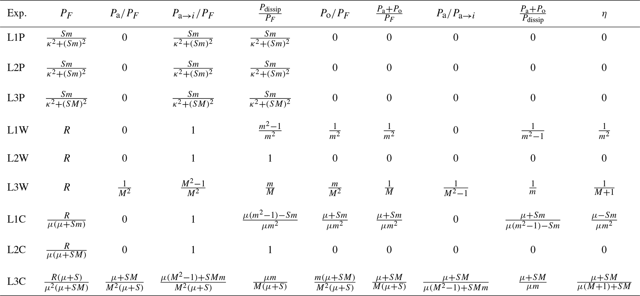
Table 1 Energy fluxes for $t\gg (SM{)}^{-\mathrm{1}},{\mathit{\mu }}^{-\mathrm{1}}$. The last column is the efficiency in the system as it compares the energy growth in the system to the energy injection. Note that for μ≫SM, LCx converges to LWx if R→Rμ².

For the L3 model, the only model that respects Newton's laws, all second-order moments have the same constant growth rate, and so the differences of these second-order moments are constant in time. They are given in Table 2.

In a perfect gas in equilibrium with molecules of different mass, the kinetic energy of each molecule, measured by the temperature, is equal on average, and heat flows on average from the hotter substance to the colder substance (second law of thermodynamics). For the forced and dissipative air–sea interaction of the L2 and L3 models, the energetic influence of the interface on the ocean is $Sm(u_{\mathrm{a}}{u}_{\mathrm{o}}-u_{\mathrm{o}}^{\mathrm{2}})$, which shows that a necessary condition for the ocean to receive energy at the interface is $u_{\mathrm{a}}^{\mathrm{2}}>u_{\mathrm{o}}^{\mathrm{2}}$. This is also true when averages are taken, $\langle u_{\mathrm{a}}^{\mathrm{2}}\rangle >\langle u_{\mathrm{o}}^{\mathrm{2}}\rangle$; it is a consequence of the Cauchy–Schwarz inequality. This is reflected in the results presented in Table 2: all entries of the third column giving $\langle u_{\mathrm{a}}^{\mathrm{2}}-u_{\mathrm{o}}^{\mathrm{2}}\rangle$ for the L2 and L3 models are positive. Due to the symmetry of the L3 model it is evident that a necessary condition for the atmosphere to receive energy at the interface is $u_{\mathrm{o}}^{\mathrm{2}}>u_{\mathrm{a}}^{\mathrm{2}}$. It is important to note that a less energetic forced atmosphere can do work on the ocean (when m>1). In the L1 model the ocean receives energy whenever $u_{\mathrm{a}}\cdot u_{\mathrm{o}}>\mathrm{0}$.

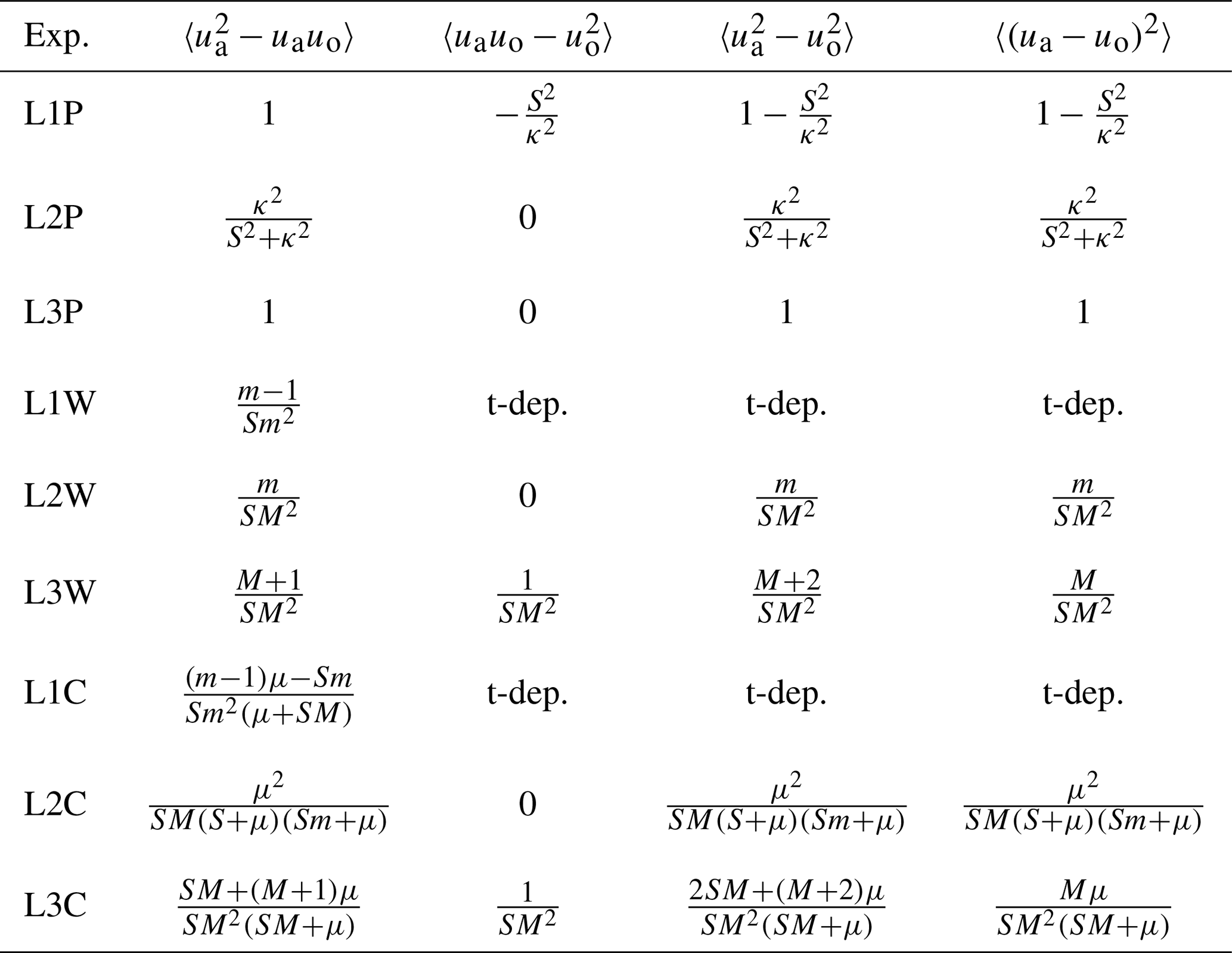
Table 2 Differences of second-order-moments of the velocity (normalised by 2(κ²+(Sm)²) for L1P and L2P, by 2(κ²+(SM)²) for L3P, by R for LxW and by R∕μ² for LxC). Note that for μ≫SM, LxC converges to LxW.

6 Fluctuation–dissipation theorem: response theory

The fluctuation–dissipation theorem (FDT) compares the response of a system subject to an external perturbation to the internal fluctuations of the system. This is related to Onsager's principle, which states that the system relaxes from a forced state to the unforced dynamics in the same manner as if the forced state were due to an internal fluctuation of the system. The expressions FDT, Onsager's principle and response theory are often interchanged in applications. Precise definitions are given in Appendixes C1 and C2. Mathematically speaking, if x(t) is the state vector of the system, the correlation matrix is $C(t,\mathrm{\Delta }t)=\langle \mathit{x}\left(t\right){\mathit{x}}^t(t+\mathrm{\Delta }t)\rangle$ and the normalised correlation matrix is $C(t,\mathrm{\Delta }t)C(t,\mathrm{0}{)}^{-\mathrm{1}}$. The average decay of an initial perturbation $\stackrel{\mathrm{‾}}{\mathit{x}}$ is given by the perturbation matrix, $\langle \mathit{x}(t+\mathrm{\Delta }t)\rangle =\mathit{\chi }(t,\mathrm{\Delta }t)\stackrel{\mathrm{‾}}{\mathit{x}}$, also called the response operator. The FDT holds if

$$\begin{array}{}\text{(20)}& C(t,\mathrm{\Delta }t)C(t,\mathrm{0}{)}^{-\mathrm{1}}=\mathit{\chi }(t,\mathrm{\Delta }t).\end{array}$$

The processes considered here are of stationary increment and the perturbation matrices are independent of the actual time t, and so are the normalised correlation matrices (see also Appendices A1–A3 and B10). The application of the FDT in the case of simple Langevin equations is discussed in Appendix C1 for the white-noise forcing and in Appendix C2 for forcing with a coloured noise. The calculations concerning the application of the FDT for the models considered here are given in Appendix B9 Eq. (B37), which show that the FDT applies in the models with white-noise forcing and coloured-noise forcing when the phase space is augmented by the variable $\stackrel{\mathrm{̃}}{F}$ representing the coloured-noise forcing. Indeed, the FDT can be verified in these models by explicitly calculating and comparing the matrices in Eq. (20). The normalised correlation matrix with a white noise forcing, which is equal to the perturbation matrix, is given for the L1 model in Eq. (A12), for the L2 model in Eq. (A19) and for the L3 model in Eq. (A26). The decay of an initial perturbation was discussed in detail at the beginning of Sect. 3. In the L1 model the ocean dynamics is undamped (see Eq. A12) and performs a random walk. In the L3 model the total momentum is undamped (see Eq. A26) and performs a random walk. The random walk has the martingale property; that is, the expectation for future values is equal to the actual value. This leads to an infinite memory in the process and infinite long correlations $\langle u_{\mathrm{total}}\left(t\right)u_{\mathrm{total}}(t+\mathrm{\Delta }t)\rangle =\langle u_{\mathrm{total}}(t{)}^{\mathrm{2}}\rangle \forall \mathrm{\Delta }t>\mathrm{0}$. Even in the case of the random walk, where the perturbation (forced or internal) does not decay, the FDT applies, as Eq. (20) is verified.

For the coloured-noise forcing the perturbation matrix in the augmented phase space is given for the L1C model in Eq. (B52), for the L2C model in Eq. (B63) and for the L3C model in Eq. (B75). The failure of the FDT for a coloured-noise forcing in a phase space consisting only of the velocities is due to the fact that the forcing has a finite correlation time, and so the future forcing is correlated with the actual velocities and the correlations of the velocities are not the same as described by the perturbation matrix. The decay of a perturbation is therefore dependent on how the perturbation was reached; that is, the system is not Markovian. This is shown in Appendix C2 and discussed in detail by Balakrishnan (1979).

The FDT relies strongly on Gaussian statistics (see e.g. Cooper and Haynes, 2011) of the variables, which is assured in linear models, but the statistics in non-linear models is clearly non-Gaussian. As, to the best of my knowledge, no analytic solution exists for the non-linear versions of the air–sea interaction models, the FDT has to be explored by numerical experiment. This will be done elsewhere.

7 Fluctuation theorem

The average states and fluxes in the different models investigated as a function of their parameters are given in Sect. 5. The probability density functions of the variables representing the atmospheric and ocean velocities are centred Gaussian variables, and therefore they are completely described by their variance. Fluxes are products of Gaussian random variables and are not Gaussian. The present section discusses instantaneous deviations from the average values, the fluctuations of the system and their persistence in time. To this end the FT (Gallavotti and Cohen, 1995a, b; Ciliberto et al., 2004) is discussed for the fluxes $P_{\mathrm{a}\to i;\mathit{\omega }}$ and $P_{i\to \mathrm{o};\mathit{\omega }}$. The FT expresses properties of these quantities evaluated along fluctuating trajectories (indexed by ω∈Ω). The FT was discovered by considering the entropy production in molecular dynamics (Evans et al., 1993), which is positive on average, according to the second law of thermodynamics. It states that heat always flows spontaneously from hotter to colder bodies. The FT specifies that this property is true on average but that locally in-time-and-space counter fluxes are present. The relation of the probability of positive versus negative fluxes of a given magnitude and their persistence in time is the subject of the FT. In the previous section averages and moments of variables were considered; the FT is concerned with the pdf.

The concepts of the FT are applied to a variety of problems and quantities and are also extended to deterministic dynamical systems. In the present work the analysis of Ciliberto et al. (2004), who tested the FT in two examples of turbulent flows in laboratory experiments, is applied. In Sect. 5 it has been shown that on average the atmosphere gains energy by the random forcing and loses energy at the interface and that the ocean gains energy at the interface. Also in the case of air–sea interaction, instantaneous fluxes can go in the opposite direction (Moulin and Wirth, 2016). The FT quantifies the asymmetry of the pdf of averages of the fluxes with respect to zero. It compares the probability of having a positive event to the probability of having a negative event of the same magnitude for averages of the fluxes over a time interval τ. Do the symmetries implied by the FT apply to the momentum fluxes $P_{\mathrm{a}\to i;\mathit{\omega }}$ and $P_{i\to \mathrm{o};\mathit{\omega }}$? The fluxes are quadratic quantities and their statistics is therefore not Gaussian. Recently a closed form of the probability density function f(Z) of the product of two correlated Gaussian variables Z=XY with vanishing means and variances ${\mathit{\sigma }}_x^{\mathrm{2}}$ and ${\mathit{\sigma }}_y^{\mathrm{2}}$ and correlation ρ has been obtained (Nadarajah and Pogány, 2016 and Gaunt, 2018) in terms of a modified Bessel function of the second kind of order zero $K_{\mathrm{0}}\left(z\right)={\int }_{\mathrm{0}}^{\mathrm{\infty }}\cos \left(z\sinh t\right)\mathrm{d}t$:

$$\begin{array}{}\text{(21)}& \begin{array}{rl}f\left(z\right)=& {\displaystyle \frac{\mathrm{1}}{\mathit{\pi }{\mathit{\sigma }}_x{\mathit{\sigma }}_y\sqrt{\mathrm{1}-{\mathit{\rho }}^{\mathrm{2}}}}}\exp \left({\displaystyle \frac{\mathit{\rho }z}{{\mathit{\sigma }}_x{\mathit{\sigma }}_y(\mathrm{1}-{\mathit{\rho }}^{\mathrm{2}})}}\right)\\ & K_{\mathrm{0}}\left({\displaystyle \frac{\left|z\right|}{{\mathit{\sigma }}_x{\mathit{\sigma }}_y(\mathrm{1}-{\mathit{\rho }}^{\mathrm{2}})}}\right).\end{array}\end{array}$$

The key quantity considered in the FT is the symmetry function:

$$\begin{array}{}\text{(22)}& S_Z\left(z\right)=\ln \left({\displaystyle \frac{f\left(z\right)}{f(-z)}}\right)=\mathit{\beta }z.\end{array}$$

For the product of two Gaussian variables S_Z(z)=βz is linear with $\mathit{\beta }=\mathrm{2}\mathit{\rho }/\left(\right(\mathrm{1}-{\mathit{\rho }}^{\mathrm{2}}\left){\mathit{\sigma }}_x{\mathit{\sigma }}_y\right)$, where Eq. (21) was used.

The normalised time average over an interval τ is denoted by

$$\begin{array}{}\text{(23)}& {\stackrel{\mathrm{‾}}{Z\left(t\right)}}^{\mathit{\tau }}={\displaystyle \frac{\mathrm{1}}{\mathit{\tau }\langle Z\left(t\right)\rangle }}\underset{\mathrm{0}}{\overset{\mathit{\tau }}{\int }}Z(t+{\mathit{\tau }}^{\prime })\mathrm{d}{\mathit{\tau }}^{\prime }.\end{array}$$

The FT holds when

$$\begin{array}{}\text{(24)}& S_{{\stackrel{\mathrm{‾}}{Z}}^{\mathit{\tau }}}\left(z\right)=\mathit{\sigma }\mathit{\tau }z\end{array}$$

in the limit of τ→∞. The variable σ is called the contraction rate (see Ciliberto et al., 2004); it depends on the problem considered.

The power the atmosphere loses at the interface $P_{\mathrm{a}\to i;\mathit{\omega }}$ and the power the ocean receives from the atmosphere at the interface $P_{i\to \mathrm{o};\mathit{\omega }}$ along a trajectory ω∈Ω are investigated. Both differ by the work dissipated at the interface (see Sect. 5). The ensemble averages of all these quantities are positive, but negative fluxes exist, even when temporal averages over time intervals of length τ are considered. The FT, as expressed by Eq. (24), states that the probability of finding a positive flux of magnitude z divided by the probability of a negative flux with the same magnitude increases exponentially with the value z and the averaging period τ.

In the problem considered here the variable ${\stackrel{\mathrm{‾}}{Z\left(t\right)}}^{\mathit{\tau }}$ is either the time-averaged work the atmosphere does on the ocean ${\stackrel{\mathrm{‾}}{P_{\mathrm{a}\to i;\mathit{\omega }}}}^{\mathit{\tau }}$, divided by its ensemble average, or the time-averaged work the ocean receives from the atmosphere ${\stackrel{\mathrm{‾}}{P_{i\to \mathrm{o};\mathit{\omega }}}}^{\mathit{\tau }}$, divided by its ensemble average. More precisely, the random variables:

$$\begin{array}{}\text{(25)}& \begin{array}{rl}& {\stackrel{\mathrm{‾}}{Z_{\mathrm{a};\mathit{\omega }}\left(t\right)}}^{\mathit{\tau }}={\displaystyle \frac{{\stackrel{\mathrm{‾}}{P_{\mathrm{a}\to i;\mathit{\omega }}\left(t\right)}}^{\mathit{\tau }}}{\langle P_{\mathrm{a}\to i;\mathit{\omega }}\left(t\right){\rangle }_{\mathrm{\Omega }}}}\mathrm{and}\\ & {\stackrel{\mathrm{‾}}{Z_{\mathrm{o};\mathit{\omega }}\left(t\right)}}^{\mathit{\tau }}={\displaystyle \frac{{\stackrel{\mathrm{‾}}{P_{i\to \mathrm{o};\mathit{\omega }}\left(t\right)}}^{\mathit{\tau }}}{\langle P_{i\to \mathrm{o};\mathit{\omega }}\left(t\right){\rangle }_{\mathrm{\Omega }}}},\end{array}\end{array}$$

for all the models are considered. Ensemble averages of the fluxes can be obtained analytically for the linear models, but I do not know their pdfs. These investigations are numerical even for the linear models considered here.

First, the L3 model is discussed. It is important to note that although $\langle P_{\mathrm{a}\to i;\mathit{\omega }}\left(t\right){\rangle }_{\mathrm{\Omega }}$ and $\langle P_{i\to \mathrm{o};\mathit{\omega }}\left(t\right){\rangle }_{\mathrm{\Omega }}$ are constant in time (after an initial spin-up of O((SM)⁻¹); see Wirth, 2018), the pdfs are not (see Fig. 2), which means that the energy transfers are non-stationary processes with a constant-in-time average value. More precisely, the pdfs of the variables ${\stackrel{\mathrm{‾}}{Z_{\mathrm{a};\mathit{\omega }}}}^{\mathit{\tau }}$ and ${\stackrel{\mathrm{‾}}{Z_{\mathrm{o};\mathit{\omega }}\left(t\right)}}^{\mathit{\tau }}$ depend on t and τ, but $\langle {\stackrel{\mathrm{‾}}{Z_{\mathrm{a};\mathit{\omega }}\left(t\right)}}^{\mathit{\tau }}{\rangle }_{\mathrm{\Omega }}$ and $\langle {\stackrel{\mathrm{‾}}{Z_{\mathrm{o};\mathit{\omega }}\left(t\right)}}^{\mathit{\tau }}{\rangle }_{\mathrm{\Omega }}$ are independent of the time t and the averaging period τ.

The parameters used in the numerical calculations are $S={\mathrm{10}}^{-\mathrm{3}}$ and m=100. Details on solving numerically the stochastic differential equations are given in Wirth (2018). The numerical results presented in Fig. 2 show that the pdfs of ${\stackrel{\mathrm{‾}}{Z_{\mathrm{a};\mathit{\omega }}\left(t\right)}}^{\mathit{\tau }}$ and ${\stackrel{\mathrm{‾}}{Z_{\mathrm{o};\mathit{\omega }}\left(t\right)}}^{\mathit{\tau }}$ for t=300, and $\mathit{\tau }=\mathrm{0},\mathrm{100}$ are non Gaussian. The exponential scaling of the symmetry function for the ocean $S_{{\stackrel{\mathrm{‾}}{Z_{\mathrm{o}}}}^{\mathit{\tau }}}\left(z\right)$ for t=300, and $\mathit{\tau }=\mathrm{0},\mathrm{100},\mathrm{200}$ is clearly present in Fig. 3. This also means that zero is a special value, which is already conspicuous in Fig. 2. The scaling exponents for $t=\mathrm{10},\mathrm{20},\mathrm{30}$ and 50 as a function of τ are given in Fig. 4, it can be verified that Eq. (24) holds, when the absolute and the averaging time exceeds the characteristic time $t,\mathit{\tau }>(SM{)}^{-\mathrm{1}}$ meaning that the FT applies asymptotically, as in Ciliberto et al. (2004). The change of slope for the different values of t is well fitted by a $\mathit{\sigma }\propto t^{-\mathrm{1}}$ law.

For the atmosphere the probability of having a negative flux P_a→i(t), that is the atmosphere receives energy at the interface due to the ocean dynamics is small even in instantaneous pdfs. Negative events in an ensemble sizes of 3×10⁷ were so few that the symmetry function could not be obtained with a sufficient accuracy.

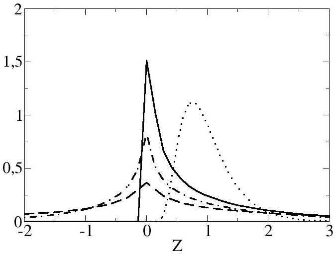
Figure 2 Probability density function of ${\stackrel{\mathrm{‾}}{Z_{\mathrm{a}/\mathrm{o};\mathit{\omega }}\left(t\right)}}^{\mathit{\tau }}$ at t=300 and τ=0, atmosphere full line, ocean dashed line, and for τ=100, atmosphere dotted line, ocean dashed-dotted line. All are clearly non-Gaussian.

Figure 3 Lin–log plot of $(S_{{\stackrel{\mathrm{‾}}{Z_{\mathrm{o}}}}^{\mathit{\tau }}}{)}^{-\mathrm{1}}$ for t=300, τ=0 full line, 10 dotted line, and 20 dashed line.

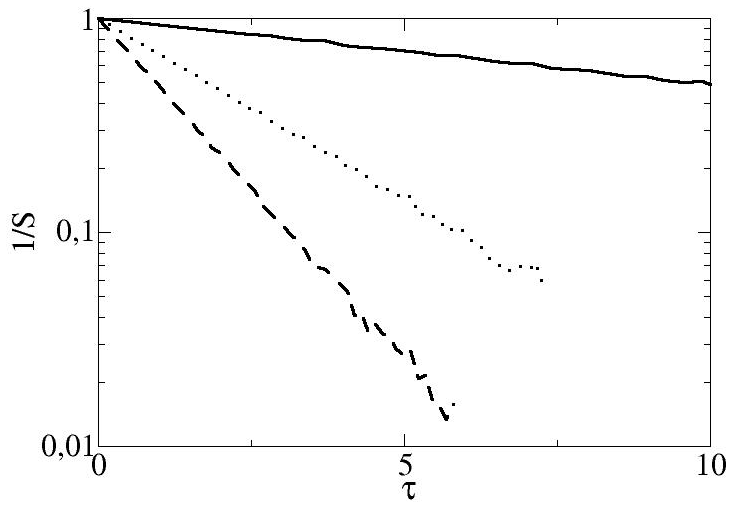
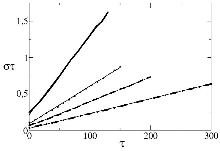
Figure 4 Scaling exponents for t=10 full line, 20 dotted line, 30 dashed line and 50 dashed-dotted line, as a function of τ and their linear fit (thin full lines); the slope is σ.

For calculations with the coloured noise model, the same parameters as in the white-noise calculations are used, and $\mathit{\mu }={\mathrm{10}}^{-\mathrm{2}}$. In this case the forcing timescale μ⁻¹ is actually slower than the atmospheric friction timescale (Sm)⁻¹ but faster than the oceanic friction timescale S⁻¹. This mimics the fact that the fast motion in the atmospheric boundary layer is forced by the slower synoptic dynamics above. The forcing time of the oceanic mixed layer is then determined by the mass ratio m between the oceanic and atmospheric layers; it is the slowest timescale. Results (not shown) from the models with coloured noise agree qualitatively with the white-noise forcing; that is, they indicate that the energy flux to the ocean obeys a FT.

Numerical integration of the L1W, L2W, L1C and L2C models show that $P_{i\to \mathrm{o};\mathit{\omega }}$ obeys the FT as in the L3 model. The atmospheric flux P_a→i(t) is always positive in the L1 and L2 models so the FT can not be considered.

8 Discussion

When ocean velocities are not considered in the models of air–sea interaction, the atmosphere loses, on average, more energy and the ocean gains more energy, as compared to when the ocean velocities are taken into account. Previous publications on the comparison of different models of air–sea interaction focus on quantitative differences. This is justified when the short-term dynamics is considered, as shown above. At longer timescales the differences are not only quantitative, but also qualitative, as for some models stationary states in the ocean, the atmosphere or in both are reached, while in others this is not the case. An example is the “eddy-killing” term (see Renault et al., 2017) that includes the ocean velocity in the shear calculation. In the short term its impact is small and can be parameterised by changing the friction coefficient. In the long term it imposes a convergence to a stationary state, when only implemented in the ocean; when implemented in the atmosphere and the ocean, it leads to a divergence in both layers, whereas neglecting it totally leads to a divergence in the ocean only. In more involved models, divergence is avoided by other processes such as non-linear interactions, increased horizontal dissipation or data assimilation, which drain energy in a different way. When these processes supplant an incomplete representation of “eddy killing”, the converged state will differ and so will the energy balance. This shows that we can not improve the L1 or L2 model by adjusting the friction parameter to obtain the behaviour of the consistent L3 model. The small differences in the short-term behaviour and the qualitative differences in the long-term behaviour between the models indicate that the choice of the model might not matter when weather or ocean forecasts are performed, but it might be crucial in climate simulations.

The magnitude of the constant growth rate is the typical growth rate of the ocean dynamics shortly after the turbulent forcing by the atmosphere has started and before dissipative processes develop to counterbalance it. It depends on the strength of the atmospheric forcing, its coherence in time and the thickness of the ocean (mixed) layer. Processes that lead to a saturation of the growth are of varying nature, space and time dependent, and typically non-linear and intermittent.

The discussion of the FDT establishes when the response to an external perturbation can be obtained from internal fluctuations of the system. In the simple system discussed here we can see analytically when it is verified and fails and how the failure can be removed by extending the phase space. Determining the response to a sudden change in the external forcing is key in many applications, such as the response of the atmospheric and oceanic planetary-boundary-layer dynamics to a change in the synoptic weather condition. The presented calculations can also be used to guide applications of the FDT to systems with large, but not infinite, time separation.

The FT concerns the transfer of energy between the atmosphere and the interface and the interface and the ocean on different timescales. The temporal down-scaling is solved when we can obtain the pdf of short-term averages from the pdf of longer-term averages. The temporal up-scaling is solved when we can obtain the pdf of long-term averages from the pdf of short-term averages. The FT relates temporal averages over different timescales and puts a large constraint on the pdfs of the averaged energy transfers over different timescales. The FT is key to understanding and modelling the climate dynamics, as in all observations and models some time-and-space averaging is present. It is not always clear what the averaging period is associated with a variable in a model. The FT gives us a hint of what to expect when passing, for example, from monthly averaged interaction/forcing to daily or hourly averages. Considering a more fundamental point of view, equilibrium statistical mechanics is based on the pdfs of the canonical ensembles. For non-equilibrium ensembles no such reference pdf is known in general (Derrida, 2007). If a FT holds, it constrains “half” of the pdf, as probabilities of positive and negative values are related. Statistical mechanics furthermore gives us the likeliness of extreme events.

The major difference between a 2-D model and a local model is that the former contains horizontal advection of momentum, while the latter does not. It is thus not clear which variable of the 2-D model has to be considered using the insight from the local models. Is it the local velocity or the velocity advected by the total-momentum mode or by the ocean dynamics, or do we have to consider coarse-grained variables for which the importance of horizontal advection is reduced? If this is the case, we have to define a coarse-graining scale that is sufficient or optimal in some sense. The FT can guide these choices.

The concepts presented here are not restricted to momentum transfer, but can also be employed to study heat exchange between the atmosphere and the ocean or other processes in the climate system with diverse characteristic timescales. Ongoing research is directed towards considering the concepts presented here in a hierarchy of models with increasing complexity and in observations. This research is of a different nature, numerical and observational, and will be described elsewhere.

Appendix A: The models

In this section the solutions of linear models L1, L2 and L3 are solved using linear algebra. The linear differential equation

$$\begin{array}{}\text{(A1)}& {\partial }_{t}u=-\mathit{\alpha }u+F\left(t\right)\end{array}$$

with initial condition u(t₀), has solutions:

$$\begin{array}{}\text{(A2)}& u\left(t\right)={\mathcal{I}}_{t_{\mathrm{0}}}^t\left(\mathit{\alpha }\right)+u\left(t_{\mathrm{0}}\right)e^{\mathit{\alpha }(t_{\mathrm{0}}-t)},\end{array}$$

with the symbol:

$$\begin{array}{}\text{(A3)}& {\mathcal{I}}_{t_{\mathrm{0}}}^t\left(\mathit{\alpha }\right)=\underset{t_{\mathrm{0}}}{\overset{t}{\int }}{e}^{\mathit{\alpha }(t^{\prime }-t)}F\left(t^{\prime }\right)\mathrm{d}{t}^{\prime }.\end{array}$$

In the multidimensional case we have

$$\begin{array}{}\text{(A4)}& {\partial }_t\mathit{u}=-P\mathit{u}+\mathit{F}F\left(t\right)=-AD{A}^{-\mathrm{1}}\mathit{u}+\mathit{F}F\left(t\right),\end{array}$$

where D is a diagonal (or Jacobi normal) matrix, F a constant coefficient vector and F(t) a time-dependent scalar forcing. The solution with initial condition u(t₀) is

$$\begin{array}{}\text{(A5)}& \mathit{u}\left(t\right)=A{\mathcal{I}}_{t_{\mathrm{0}}}^t\left(D\right)A^{-\mathrm{1}}\mathit{F}+A{e}^{D(t_{\mathrm{0}}-t)}{A}^{-\mathrm{1}}\mathit{u}\left(t_{\mathrm{0}}\right).\end{array}$$

Note that in all our applications α and the eigenvalues of D are positive or zero.

A1 Model L1

The system is forced and damped and the atmospheric dynamics acts on the ocean without considering the ocean velocity. A coupling which is still used in some climate models.

$$\begin{array}{}\text{(A6)}& {\displaystyle }{\partial }_t{u}_{\mathrm{a}}=-Sm{u}_{\mathrm{a}}+F_{\mathrm{a}}\text{(A7)}& {\displaystyle }{\partial }_t{u}_{\mathrm{o}}=S{u}_{\mathrm{a}}+F_{\mathrm{o}}\text{(A8)}& {\displaystyle }{\partial }_t\left(\begin{array}{c}{u}_{\mathrm{a}}\\ u_{\mathrm{o}}\end{array}\right)=\left(\begin{array}{cc}-Sm& \mathrm{0}\\ S& \mathrm{0}\end{array}\right)\left(\begin{array}{c}{u}_{\mathrm{a}}\\ u_{\mathrm{o}}\end{array}\right)+\left(\begin{array}{c}{F}_{\mathrm{a}}\\ F_{\mathrm{o}}\end{array}\right)\text{(A9)}& {\displaystyle }{\mathit{\lambda }}_{\mathrm{1}}=-Sm,e_{\mathrm{1}}=\left(\begin{array}{c}m\\ -\mathrm{1}\end{array}\right);{\mathit{\lambda }}_{\mathrm{2}}=\mathrm{0},e_{\mathrm{2}}=\left(\begin{array}{c}\mathrm{0}\\ \mathrm{1}\end{array}\right)\text{(A10)}& {\displaystyle }\begin{array}{rl}P=AD{A}^{-\mathrm{1}}& =\left(\begin{array}{cc}-Sm& \mathrm{0}\\ S& \mathrm{0}\end{array}\right)\\ & =\left(\begin{array}{cc}m& \mathrm{0}\\ -\mathrm{1}& \mathrm{1}\end{array}\right)\left(\begin{array}{cc}-Sm& \mathrm{0}\\ \mathrm{0}& \mathrm{0}\end{array}\right)\left(\begin{array}{cc}{m}^{-\mathrm{1}}& \mathrm{0}\\ m^{-\mathrm{1}}& \mathrm{1}\end{array}\right).\end{array}\end{array}$$

The solution is

$$\begin{array}{}\text{(A11)}& \begin{array}{rl}\left(\begin{array}{c}{u}_{\mathrm{a}}\left(t\right)\\ u_{\mathrm{o}}\left(t\right)\end{array}\right)& =A{\mathcal{I}}_{t_{\mathrm{0}}}^t\left(D\right)A^{-\mathrm{1}}\left(\begin{array}{c}{F}_{\mathrm{a}}\\ F_{\mathrm{o}}\end{array}\right)\\ & =A\left(\begin{array}{cc}{\mathcal{I}}_{t_{\mathrm{0}}}^t\left(Sm\right)& \mathrm{0}\\ \mathrm{0}& {\mathcal{I}}_{t_{\mathrm{0}}}^t\left(\mathrm{0}\right)\end{array}\right)A^{-\mathrm{1}}\left(\begin{array}{c}{F}_{\mathrm{a}}\\ F_{\mathrm{o}}\end{array}\right)\\ & =\left(\begin{array}{cc}{\mathcal{I}}_{t_{\mathrm{0}}}^t\left(Sm\right)& \mathrm{0}\\ \left[-{\mathcal{I}}_{t_{\mathrm{0}}}^t\left(Sm\right)+{\mathcal{I}}_{t_{\mathrm{0}}}^t\left(\mathrm{0}\right)\right]/m& {\mathcal{I}}_{t_{\mathrm{0}}}^t\left(\mathrm{0}\right)\end{array}\right)\left(\begin{array}{c}{F}_{\mathrm{a}}\\ F_{\mathrm{o}}\end{array}\right).\end{array}\end{array}$$

In the absence of forcing, an initial perturbation at Δt=0, $({\stackrel{\mathrm{‾}}{u}}_{\mathrm{a}},{\stackrel{\mathrm{‾}}{u}}_{\mathrm{o}})$, evolves as

$$\begin{array}{}\text{(A12)}& \left(\begin{array}{c}{u}_{\mathrm{a}}^P\left(\mathrm{\Delta }t\right)\\ u_{\mathrm{o}}^P\left(\mathrm{\Delta }t\right)\end{array}\right)=\left(\begin{array}{cc}{e}^{-Sm\mathrm{\Delta }t}& \mathrm{0}\\ \frac{\mathrm{1}-e^{-Sm\mathrm{\Delta }t}}{m}& \mathrm{1}\end{array}\right)\left(\begin{array}{c}{\stackrel{\mathrm{‾}}{u}}_{\mathrm{a}}\\ {\stackrel{\mathrm{‾}}{u}}_{\mathrm{o}}\end{array}\right).\end{array}$$

Note that the perturbation matrix above, $\mathit{\chi }\left(\mathrm{\Delta }t\right)=A\exp \left(D\mathrm{\Delta }t\right)A^{-\mathrm{1}}$, is independent of the time t.

A2 Model L2

The system is forced with damping and the atmospheric dynamics forces the ocean, ocean velocity is taken into account for the ocean dynamics but not in the atmospheric dynamics (Newton's third law is not respected).

$$\begin{array}{}\text{(A13)}& {\displaystyle }{\partial }_t{u}_{\mathrm{a}}=-Sm{u}_{\mathrm{a}}+F_{\mathrm{a}}\text{(A14)}& {\displaystyle }{\partial }_t{u}_{\mathrm{o}}=S(u_{\mathrm{a}}-u_{\mathrm{o}})+F_{\mathrm{o}}\text{(A15)}& {\displaystyle }{\partial }_t\left(\begin{array}{c}{u}_{\mathrm{a}}\\ u_{\mathrm{o}}\end{array}\right)=\left(\begin{array}{cc}-Sm& \mathrm{0}\\ S& -S\end{array}\right)\left(\begin{array}{c}{u}_{\mathrm{a}}\\ u_{\mathrm{o}}\end{array}\right)+\left(\begin{array}{c}{F}_{\mathrm{a}}\\ F_{\mathrm{o}}\end{array}\right)\text{(A16)}& {\displaystyle }{\mathit{\lambda }}_{\mathrm{1}}=-Sm,e_{\mathrm{1}}=\left(\begin{array}{c}m-\mathrm{1}\\ -\mathrm{1}\end{array}\right);{\mathit{\lambda }}_{\mathrm{2}}=-S,e_{\mathrm{2}}=\left(\begin{array}{c}\mathrm{0}\\ \mathrm{1}\end{array}\right)\text{(A17)}& {\displaystyle }\begin{array}{rl}P=AD{A}^{-\mathrm{1}}=& \left(\begin{array}{cc}-Sm& \mathrm{0}\\ S& -S\end{array}\right)=\left(\begin{array}{cc}m-\mathrm{1}& \mathrm{0}\\ -\mathrm{1}& \mathrm{1}\end{array}\right)\\ & \left(\begin{array}{cc}-Sm& \mathrm{0}\\ \mathrm{0}& -S\end{array}\right)\left(\begin{array}{cc}(m-\mathrm{1}{)}^{-\mathrm{1}}& \mathrm{0}\\ (m-\mathrm{1}{)}^{-\mathrm{1}}& \mathrm{1}\end{array}\right).\end{array}\end{array}$$

The solution is

$$\begin{array}{}\text{(A18)}& {\displaystyle }\begin{array}{rl}& \left(\begin{array}{c}{u}_{\mathrm{a}}\left(t\right)\\ u_{\mathrm{o}}\left(t\right)\end{array}\right)=A{\mathcal{I}}_{t_{\mathrm{0}}}^t\left(D\right)A^{-\mathrm{1}}\left(\begin{array}{c}{F}_{\mathrm{a}}\\ F_{\mathrm{o}}\end{array}\right)\\ & \left(\begin{array}{c}{u}_{\mathrm{a}}\left(t\right)\\ u_{\mathrm{o}}\left(t\right)\end{array}\right)=A\left(\begin{array}{cc}{\mathcal{I}}_{t_{\mathrm{0}}}^t\left(Sm\right)& \mathrm{0}\\ \mathrm{0}& {\mathcal{I}}_{t_{\mathrm{0}}}^t\left(S\right)\end{array}\right)A^{-\mathrm{1}}\left(\begin{array}{c}{F}_{\mathrm{a}}\\ F_{\mathrm{o}}\end{array}\right)\\ & =\left(\begin{array}{cc}{\mathcal{I}}_{t_{\mathrm{0}}}^t\left(Sm\right)& \mathrm{0}\\ \left[-{\mathcal{I}}_{t_{\mathrm{0}}}^t\left(Sm\right)+{\mathcal{I}}_{t_{\mathrm{0}}}^t\left(S\right)\right]/(m-\mathrm{1})& {\mathcal{I}}_{t_{\mathrm{0}}}^t\left(S\right)\end{array}\right)\left(\begin{array}{c}{F}_{\mathrm{a}}\\ F_{\mathrm{o}}\end{array}\right).\end{array}\end{array}$$

In the absence of forcing, an initial perturbation at Δt=0, $({\stackrel{\mathrm{‾}}{u}}_{\mathrm{a}},{\stackrel{\mathrm{‾}}{u}}_{\mathrm{o}})$, evolves as

$$\begin{array}{}\text{(A19)}& \left(\begin{array}{c}{u}_{\mathrm{a}}^P\left(\mathrm{\Delta }t\right)\\ u_{\mathrm{o}}^P\left(\mathrm{\Delta }t\right)\end{array}\right)=\left(\begin{array}{cc}{e}^{-Sm\mathrm{\Delta }t}& \mathrm{0}\\ \frac{e^{-S\mathrm{\Delta }t}-e^{-Sm\mathrm{\Delta }t}}{m-\mathrm{1}}& e^{-S\mathrm{\Delta }t}\end{array}\right)\left(\begin{array}{c}{\stackrel{\mathrm{‾}}{u}}_{\mathrm{a}}\\ {\stackrel{\mathrm{‾}}{u}}_{\mathrm{o}}\end{array}\right).\end{array}$$

Note that the perturbation matrix above: $\mathit{\chi }\left(\mathrm{\Delta }t\right)=A\exp \left(D\mathrm{\Delta }t\right)A^{-\mathrm{1}}$, is independent of the time t.

A3 Model L3

The atmosphere is forced with damping and the atmospheric dynamics forces the ocean, the ocean velocity is taken into account.

$$\begin{array}{}\text{(A20)}& {\displaystyle }{\partial }_t{u}_{\mathrm{a}}=Sm(u_{\mathrm{o}}-u_{\mathrm{a}})+F_{\mathrm{a}}\text{(A21)}& {\displaystyle }{\partial }_t{u}_{\mathrm{o}}=S(u_{\mathrm{a}}-u_{\mathrm{o}})+F_{\mathrm{o}}\text{(A22)}& {\displaystyle }{\partial }_t\left(\begin{array}{c}{u}_{\mathrm{a}}\\ u_{\mathrm{o}}\end{array}\right)=\left(\begin{array}{cc}-Sm& Sm\\ S& -S\end{array}\right)\left(\begin{array}{c}{u}_{\mathrm{a}}\\ u_{\mathrm{o}}\end{array}\right)+\left(\begin{array}{c}{F}_{\mathrm{a}}\\ F_{\mathrm{o}}\end{array}\right)\text{(A23)}& {\displaystyle }{\mathit{\lambda }}_{\mathrm{1}}=-SM,e_{\mathrm{1}}=\left(\begin{array}{c}m\\ -\mathrm{1}\end{array}\right);{\mathit{\lambda }}_{\mathrm{2}}=\mathrm{0},e_{\mathrm{2}}=\left(\begin{array}{c}\mathrm{1}\\ \mathrm{1}\end{array}\right).\end{array}$$

The first eigenvector corresponds to the shear mode and the second to the total-momentum mode.

$$\begin{array}{}\text{(A24)}& \begin{array}{rl}P=AD{A}^{-\mathrm{1}}=& \left(\begin{array}{cc}-Sm& Sm\\ S& -S\end{array}\right)=\left(\begin{array}{cc}m& \mathrm{1}\\ -\mathrm{1}& \mathrm{1}\end{array}\right)\\ & \left(\begin{array}{cc}-SM& \mathrm{0}\\ \mathrm{0}& \mathrm{0}\end{array}\right){\displaystyle \frac{\mathrm{1}}{M}}\left(\begin{array}{cc}\mathrm{1}& -\mathrm{1}\\ \mathrm{1}& m\end{array}\right).\end{array}\end{array}$$

The solution is

$$\begin{array}{}\text{(A25)}& {\displaystyle }\begin{array}{rl}& \left(\begin{array}{c}{u}_{\mathrm{a}}\left(t\right)\\ u_{\mathrm{o}}\left(t\right)\end{array}\right)=A{\mathcal{I}}_{t_{\mathrm{0}}}^t\left(D\right)A^{-\mathrm{1}}\left(\begin{array}{c}{F}_{\mathrm{a}}\\ F_{\mathrm{o}}\end{array}\right),\\ & \left(\begin{array}{c}{u}_{\mathrm{a}}\left(t\right)\\ u_{\mathrm{o}}\left(t\right)\end{array}\right)=A\left(\begin{array}{cc}{\mathcal{I}}_{t_{\mathrm{0}}}^t\left(SM\right)& \mathrm{0}\\ \mathrm{0}& {\mathcal{I}}_{t_{\mathrm{0}}}^t\left(\mathrm{0}\right)\end{array}\right)A^{-\mathrm{1}}\left(\begin{array}{c}{F}_{\mathrm{a}}\\ F_{\mathrm{o}}\end{array}\right)\\ & ={\displaystyle \frac{\mathrm{1}}{M}}\left(\begin{array}{cc}m{\mathcal{I}}_{t_{\mathrm{0}}}^t\left(SM\right)+{\mathcal{I}}_{t_{\mathrm{0}}}^t\left(\mathrm{0}\right)& -m{\mathcal{I}}_{t_{\mathrm{0}}}^t\left(SM\right)+m{\mathcal{I}}_{t_{\mathrm{0}}}^t\left(\mathrm{0}\right)\\ -{\mathcal{I}}_{t_{\mathrm{0}}}^t\left(SM\right)+{\mathcal{I}}_{t_{\mathrm{0}}}^t\left(\mathrm{0}\right)& {\mathcal{I}}_{t_{\mathrm{0}}}^t\left(SM\right)+m{\mathcal{I}}_{t_{\mathrm{0}}}^t\left(\mathrm{0}\right)\end{array}\right)\left(\begin{array}{c}{F}_{\mathrm{a}}\\ F_{\mathrm{o}}\end{array}\right).\end{array}\end{array}$$

In the absence of forcing, an initial perturbation at Δt=0, $({\stackrel{\mathrm{‾}}{u}}_{\mathrm{a}},{\stackrel{\mathrm{‾}}{u}}_{\mathrm{o}})$, evolves as

$$\begin{array}{}\text{(A26)}& \left(\begin{array}{c}{u}_{\mathrm{a}}^P\left(\mathrm{\Delta }t\right)\\ u_{\mathrm{o}}^P\left(\mathrm{\Delta }t\right)\end{array}\right)={\displaystyle \frac{\mathrm{1}}{M}}\left(\begin{array}{cc}\mathrm{1}+m{e}^{-SM\mathrm{\Delta }t}& m(\mathrm{1}-e^{-SM\mathrm{\Delta }t})\\ \mathrm{1}-e^{-SM\mathrm{\Delta }t}& m+e^{-SM\mathrm{\Delta }t}\end{array}\right)\left(\begin{array}{c}{\stackrel{\mathrm{‾}}{u}}_{\mathrm{a}}\\ {\stackrel{\mathrm{‾}}{u}}_{\mathrm{o}}\end{array}\right).\end{array}$$

Note that the perturbation matrix above: $\mathit{\chi }\left(\mathrm{\Delta }t\right)=A\exp \left(D\mathrm{\Delta }t\right)A^{-\mathrm{1}}$, is independent of the time t.

Appendix B: Experiments

In all experiments only the atmosphere is forced, F_o=0. Note that in the L3 model the atmosphere and the ocean are treated similarly and they only differ by the mass ratio m. The dynamics due to a forcing of the ocean can be represented by choosing m<1 and interchanging the subscripts. The dynamics of a forcing of the ocean and atmosphere can be obtained by adding a model forced by the ocean and the same model forced by the atmosphere due to the linearity of the model.

B1 Constant forcing

In this Appendix F_a=1 and F_o=0. Put into Eq. (A3), this leads to

$$\begin{array}{}\text{(B1)}& {\displaystyle }{\mathcal{I}}_{t_{\mathrm{0}}}^t\left(\mathrm{0}\right)=t-t_{\mathrm{0}},\text{(B2)}& {\displaystyle }{\mathcal{I}}_{t_{\mathrm{0}}}^t\left(\mathit{\alpha }\right)={\displaystyle \frac{\mathrm{1}}{\mathit{\alpha }}}(\mathrm{1}-\exp (-\mathit{\alpha }(t-t_{\mathrm{0}})\left)\right),\mathrm{if}\mathit{\alpha }\ne \mathrm{0}.\end{array}$$

The solutions for the different models are the following.

B2 Experiment L1K

$$\begin{array}{}\text{(B3)}& \left(\begin{array}{c}{u}_{\mathrm{a}}\left(t\right)\\ u_{\mathrm{o}}\left(t\right)\end{array}\right)={\displaystyle \frac{\mathrm{1}}{Sm}}\left(\begin{array}{c}\mathrm{1}-\exp (-Sm(t-t_{\mathrm{0}}\left)\right)\\ \left[Sm\right(t-t_{\mathrm{0}})-\mathrm{1}+\exp (-Sm(t-t_{\mathrm{0}})\left)\right]/m\end{array}\right).\end{array}$$

The Taylor series expansion for small times $(t-t_{\mathrm{0}})\ll (Sm{)}^{-\mathrm{1}}$ is

$$\begin{array}{}\text{(B4)}& \left(\begin{array}{c}{u}_{\mathrm{a}}\left(t\right)\\ u_{\mathrm{o}}\left(t\right)\end{array}\right)=\left(\begin{array}{c}t-t_{\mathrm{0}}-\frac{Sm}{\mathrm{2}}(t-t_{\mathrm{0}}{)}^{\mathrm{2}}+\frac{(Sm{)}^{\mathrm{2}}}{\mathrm{6}}(t-t_{\mathrm{0}}{)}^{\mathrm{3}}-\mathrm{\dots }\\ \frac{S}{\mathrm{2}}(t-t_{\mathrm{0}}{)}^{\mathrm{2}}-\frac{S^{\mathrm{2}}m}{\mathrm{6}}(t-t_{\mathrm{0}}{)}^{\mathrm{3}}+\frac{S^{\mathrm{3}}{m}^{\mathrm{2}}}{\mathrm{24}}(t-t_{\mathrm{0}}{)}^{\mathrm{4}}-\mathrm{\dots }\end{array}\right).\end{array}$$

Asymptotics for large times $(t-t_{\mathrm{0}})\gg (Sm{)}^{-\mathrm{1}}$:

$$\begin{array}{}\text{(B5)}& \left(\begin{array}{c}{u}_{\mathrm{a}}\left(t\right)\\ u_{\mathrm{o}}\left(t\right)\end{array}\right)=\left(\begin{array}{c}\frac{\mathrm{1}}{Sm}\\ \frac{t-t_{\mathrm{0}}}{m}-\frac{\mathrm{1}}{S{m}^{\mathrm{2}}}\end{array}\right).\end{array}$$

B3 Experiment L2K

$$\begin{array}{}\text{(B6)}& \begin{array}{rl}& \left(\begin{array}{c}{u}_{\mathrm{a}}\left(t\right)\\ u_{\mathrm{o}}\left(t\right)\end{array}\right)=\\ & \left(\begin{array}{c}[\mathrm{1}-\exp (-Sm(t-t_{\mathrm{0}})\left)\right]/\left(Sm\right)\\ \left[\mathrm{1}-\exp (-S(t-t_{\mathrm{0}}\left)\right)-(\mathrm{1}-\exp (-Sm(t-t_{\mathrm{0}}))/m\right]/\left(S\right(m-\mathrm{1}\left)\right)\end{array}\right).\end{array}\end{array}$$

The Taylor-series expansion for small times $(t-t_{\mathrm{0}})\ll (Sm{)}^{-\mathrm{1}}$ is

$$\begin{array}{}\text{(B7)}& \begin{array}{rl}& \left(\begin{array}{c}{u}_{\mathrm{a}}\left(t\right)\\ u_{\mathrm{o}}\left(t\right)\end{array}\right)=\\ & \left(\begin{array}{c}t-t_{\mathrm{0}}-\frac{Sm}{\mathrm{2}}(t-t_{\mathrm{0}}{)}^{\mathrm{2}}+\frac{(Sm{)}^{\mathrm{2}}}{\mathrm{6}}(t-t_{\mathrm{0}}{)}^{\mathrm{3}}-\mathrm{\dots }\\ \frac{S}{\mathrm{2}}(t-t_{\mathrm{0}}{)}^{\mathrm{2}}-\frac{S^{\mathrm{2}}M}{\mathrm{6}}(t-t_{\mathrm{0}}{)}^{\mathrm{3}}+\frac{S^{\mathrm{3}}(m^{\mathrm{2}}+m+\mathrm{1})}{\mathrm{24}}(t-t_{\mathrm{0}}{)}^{\mathrm{4}}-\mathrm{\dots }\end{array}\right).\end{array}\end{array}$$

Asymptotics for large times $(t-t_{\mathrm{0}})\gg S^{-\mathrm{1}}$:

$$\begin{array}{}\text{(B8)}& \left(\begin{array}{c}{u}_{\mathrm{a}}\left(t\right)\\ u_{\mathrm{o}}\left(t\right)\end{array}\right)=\left(\begin{array}{c}\frac{\mathrm{1}}{Sm}\\ \frac{\mathrm{1}}{Sm}\end{array}\right).\end{array}$$

.

B4 Experiment L3K

$$\begin{array}{}\text{(B9)}& \left(\begin{array}{c}{u}_{\mathrm{a}}\left(t\right)\\ u_{\mathrm{o}}\left(t\right)\end{array}\right)={\displaystyle \frac{\mathrm{1}}{M}}\left(\begin{array}{c}t-t_{\mathrm{0}}+(\mathrm{1}-\exp (-SM(t-t_{\mathrm{0}})\left)\right)m/\left(SM\right)\\ t-t_{\mathrm{0}}-(\mathrm{1}-\exp (-SM(t-t_{\mathrm{0}})\left)\right)/\left(SM\right)\end{array}\right)\end{array}$$

The Taylor-series expansion for small times $(t-t_{\mathrm{0}})\ll (Sm{)}^{-\mathrm{1}}$ is

$$\begin{array}{}\text{(B10)}& \begin{array}{rl}& \left(\begin{array}{c}{u}_{\mathrm{a}}\left(t\right)\\ u_{\mathrm{o}}\left(t\right)\end{array}\right)=\\ & \left(\begin{array}{c}t-t_{\mathrm{0}}-\frac{Sm}{\mathrm{2}}(t-t_{\mathrm{0}}{)}^{\mathrm{2}}+\frac{S^{\mathrm{2}}mM}{\mathrm{6}}(t-t_{\mathrm{0}}{)}^{\mathrm{3}}-\mathrm{\dots }\\ \frac{S}{\mathrm{2}}(t-t_{\mathrm{0}}{)}^{\mathrm{2}}-\frac{S^{\mathrm{2}}M}{\mathrm{6}}(t-t_{\mathrm{0}}{)}^{\mathrm{3}}+\frac{S^{\mathrm{3}}{M}^{\mathrm{2}}}{\mathrm{24}}(t-t_{\mathrm{0}}{)}^{\mathrm{4}}-\mathrm{\dots }\end{array}\right)\end{array}\end{array}$$

Asymptotics for large times $(t-t_{\mathrm{0}})\gg (SM{)}^{-\mathrm{1}}$:

$$\begin{array}{}\text{(B11)}& \left(\begin{array}{c}{u}_{\mathrm{a}}\left(t\right)\\ u_{\mathrm{o}}\left(t\right)\end{array}\right)=\left(\begin{array}{c}\frac{t-t_{\mathrm{0}}}{M}+\frac{m}{S{M}^{\mathrm{2}}}\\ \frac{t-t_{\mathrm{0}}}{M}-\frac{\mathrm{1}}{S{M}^{\mathrm{2}}}\end{array}\right)\end{array}$$

B5 Periodic forcing

In this Appendix F_a=cos (κt). Put into Eq. (A3), and starting the integration at $t_{\mathrm{0}}=-\mathrm{\infty }$ (ignoring transients), this leads to

$$\begin{array}{}\text{(B12)}& {\mathcal{I}}_{-\mathrm{\infty }}^t\left(\mathit{\alpha }\right)={\displaystyle \frac{\mathrm{1}}{{\mathit{\alpha }}^{\mathrm{2}}+{\mathit{\kappa }}^{\mathrm{2}}}}\left(\mathit{\kappa }\sin \right(\mathit{\kappa }t)+\mathit{\alpha }\cos (\mathit{\kappa }t\left)\right).\end{array}$$

B6 Experiment L1P

The solution is

$$\begin{array}{}\text{(B13)}& \left(\begin{array}{c}{u}_{\mathrm{a}}\left(t\right)\\ u_{\mathrm{o}}\left(t\right)\end{array}\right)={\displaystyle \frac{\mathrm{1}}{(Sm{)}^{\mathrm{2}}+{\mathit{\kappa }}^{\mathrm{2}}}}\left(\begin{array}{c}\left(\mathit{\kappa }\sin \right(\mathit{\kappa }t)+Sm\cos (\mathit{\kappa }t\left)\right)\\ S/\mathit{\kappa }\left(Sm\sin \right(\mathit{\kappa }t)-\mathit{\kappa }\cos (\mathit{\kappa }t\left)\right)\end{array}\right).\end{array}$$

The averages over one period $\mathit{\tau }=\mathrm{2}\mathit{\pi }/\mathit{\kappa }$ are denoted by 〈.〉_τ. First-order moments all vanish, and for the second-order moments we get

$$\begin{array}{}\text{(B14)}& \begin{array}{rl}\mathrm{2}\langle u_{\mathrm{a}}^{\mathrm{2}}{\rangle }_{\mathit{\tau }}& ={\displaystyle \frac{\mathrm{1}}{(Sm{)}^{\mathrm{2}}+{\mathit{\kappa }}^{\mathrm{2}}}},\\ \mathrm{2}\langle u_{\mathrm{o}}^{\mathrm{2}}{\rangle }_{\mathit{\tau }}& ={\displaystyle \frac{S^{\mathrm{2}}}{{\mathit{\kappa }}^{\mathrm{2}}\left(\right(Sm{)}^{\mathrm{2}}+{\mathit{\kappa }}^{\mathrm{2}})}},\\ {\displaystyle \frac{\langle u_{\mathrm{o}}^{\mathrm{2}}{\rangle }_{\mathit{\tau }}}{\langle u_{\mathrm{a}}^{\mathrm{2}}{\rangle }_{\mathit{\tau }}}}& ={\displaystyle \frac{S^{\mathrm{2}}}{{\mathit{\kappa }}^{\mathrm{2}}}},\\ \langle u_{\mathrm{a}}{u}_{\mathrm{o}}{\rangle }_{\mathit{\tau }}& =\mathrm{0}.\end{array}\end{array}$$

B7 Experiment L2P

$$\begin{array}{}\text{(B15)}& {\displaystyle }{u}_{\mathrm{a}}={\displaystyle \frac{\mathrm{1}}{(Sm{)}^{\mathrm{2}}+{\mathit{\kappa }}^{\mathrm{2}}}}\left[\mathit{\kappa }\sin \right(\mathit{\kappa }t)+Sm\cos (\mathit{\kappa }t\left)\right]\text{(B16)}& {\displaystyle }\begin{array}{rl}{u}_{\mathrm{o}}=& {\displaystyle \frac{S}{\left(\right(Sm{)}^{\mathrm{2}}+{\mathit{\kappa }}^{\mathrm{2}}\left)\right(S^{\mathrm{2}}+{\mathit{\kappa }}^{\mathrm{2}})}}\left[SM\mathit{\kappa }\sin \right(\mathit{\kappa }t)\\ & +(S^{\mathrm{2}}m-{\mathit{\kappa }}^{\mathrm{2}})\cos \left(\mathit{\kappa }t\right)]\end{array}\end{array}$$

$$\begin{array}{c}{\displaystyle }\mathrm{2}\langle u_{\mathrm{a}}^{\mathrm{2}}{\rangle }_{\mathit{\tau }}={\displaystyle \frac{\mathrm{1}}{(Sm{)}^{\mathrm{2}}+{\mathit{\kappa }}^{\mathrm{2}}}}\\ {\displaystyle }\mathrm{2}\langle u_{\mathrm{o}}^{\mathrm{2}}{\rangle }_{\mathit{\tau }}=\mathrm{2}\langle u_{\mathrm{a}}{u}_{\mathrm{o}}{\rangle }_{\mathit{\tau }}={\displaystyle \frac{S^{\mathrm{2}}}{\left(\right(Sm{)}^{\mathrm{2}}+{\mathit{\kappa }}^{\mathrm{2}}\left)\right(S^{\mathrm{2}}+{\mathit{\kappa }}^{\mathrm{2}})}}\\ {\displaystyle \frac{\langle u_{\mathrm{o}}^{\mathrm{2}}{\rangle }_{\mathit{\tau }}}{\langle u_{\mathrm{a}}^{\mathrm{2}}{\rangle }_{\mathit{\tau }}}}={\displaystyle \frac{S^{\mathrm{2}}}{S^{\mathrm{2}}+{\mathit{\kappa }}^{\mathrm{2}}}}\end{array}$$

B8 Experiment L3P

$$\begin{array}{}\text{(B17)}& \begin{array}{rl}{u}_{\mathrm{a}}\left(t\right)& ={\displaystyle \frac{\mathrm{1}}{M}}(u_t+m{u}_s)\\ & ={\displaystyle \frac{\mathrm{1}}{{\mathit{\kappa }}^{\mathrm{2}}+(SM{)}^{\mathrm{2}}}}\left[{\displaystyle \frac{{\mathit{\kappa }}^{\mathrm{2}}+S^{\mathrm{2}}M}{\mathit{\kappa }}}\sin \left(\mathit{\kappa }t\right)+Sm\cos \left(\mathit{\kappa }t\right)\right],\\ u_{\mathrm{o}}\left(t\right)& ={\displaystyle \frac{\mathrm{1}}{M}}(u_t-u_s)\\ & ={\displaystyle \frac{S}{\mathit{\kappa }({\mathit{\kappa }}^{\mathrm{2}}+(SM{)}^{\mathrm{2}})}}\left[SM\sin \left(\mathit{\kappa }t\right)-\mathit{\kappa }\cos \left(\mathit{\kappa }t\right)\right],\end{array}\end{array}$$

which leads to

$$\begin{array}{}\text{(B18)}& {\displaystyle }\mathrm{2}\langle u_{\mathrm{a}}^{\mathrm{2}}{\rangle }_{\mathit{\tau }}={\displaystyle \frac{\mathrm{1}}{{\mathit{\kappa }}^{\mathrm{2}}+(SM{)}^{\mathrm{2}}}}{\displaystyle \frac{{\mathit{\kappa }}^{\mathrm{2}}+S^{\mathrm{2}}}{{\mathit{\kappa }}^{\mathrm{2}}}},\text{(B19)}& {\displaystyle }\mathrm{2}\langle u_{\mathrm{o}}^{\mathrm{2}}{\rangle }_{\mathit{\tau }}=\mathrm{2}\langle u_{\mathrm{a}}{u}_{\mathrm{o}}{\rangle }_t={\displaystyle \frac{\mathrm{1}}{{\mathit{\kappa }}^{\mathrm{2}}+(SM{)}^{\mathrm{2}}}}{\displaystyle \frac{S^{\mathrm{2}}}{{\mathit{\kappa }}^{\mathrm{2}}}},\text{(B20)}& {\displaystyle \frac{\langle u_{\mathrm{o}}^{\mathrm{2}}{\rangle }_{\mathit{\tau }}}{\langle u_{\mathrm{a}}^{\mathrm{2}}{\rangle }_{\mathit{\tau }}}}={\displaystyle \frac{S^{\mathrm{2}}}{{\mathit{\kappa }}^{\mathrm{2}}+S^{\mathrm{2}}}}.\end{array}$$

B9 Random walk and Ornstein–Uhlenbeck process

The following identities are used:

$$\begin{array}{}\text{(B21)}& {\displaystyle }\underset{-\mathrm{\infty }}{\overset{t}{\int }}\mathit{\delta }(t-t^{\prime })\mathrm{d}{t}^{\prime }=\mathrm{1}/\mathrm{2},\text{(B22)}& {\displaystyle }\underset{t_{\mathrm{0}}}{\overset{t}{\int }}\underset{t_{\mathrm{0}}}{\overset{t}{\int }}\mathit{\delta }(t^{\prime \prime }-t^{\prime })\mathrm{d}{t}^{\prime \prime }\mathrm{d}{t}^{\prime }=t-t_{\mathrm{0}},\text{(B23)}& {\displaystyle }\langle F_{\mathit{\omega }}\left(t\right){\rangle }_{\mathrm{\Omega }}=\mathrm{0},\text{(B24)}& {\displaystyle }\langle F_{\mathit{\omega }}\left(t^{\prime }\right)F_{\mathit{\omega }}\left(t^{\prime \prime }\right){\rangle }_{\mathrm{\Omega }}=\mathrm{2}R\mathit{\delta }(t^{\prime \prime }-t^{\prime }).\end{array}$$

In the sequel the subscript ω is omitted. Below are the equations for a random walk u_R and an Ornstein–Uhlenbeck process u_O, the solution of a Langevin equation.

$$\begin{array}{}\text{(B25)}& {\displaystyle }{\partial }_t{u}_{\mathrm{R}}=F\text{(B26)}& {\displaystyle }{\partial }_t{u}_{\mathrm{O}}=-S{u}_{\mathrm{O}}+F\end{array}$$

Solutions starting from rest at t₀, $u_{\mathrm{R}}\left(t_{\mathrm{0}}\right)=u_{\mathrm{O}}\left(t_{\mathrm{0}}\right)=\mathrm{0}$, are

$$\begin{array}{}\text{(B27)}& {\displaystyle }{u}_{\mathrm{R}}\left(t\right)=\underset{t_{\mathrm{0}}}{\overset{t}{\int }}F\left(t^{\prime }\right)\mathrm{d}{t}^{\prime },\text{(B28)}& {\displaystyle }{u}_{\mathrm{O}}\left(t\right)=\underset{t_{\mathrm{0}}}{\overset{t}{\int }}{e}^{S(t^{\prime }-t)}F\left(t^{\prime }\right)\mathrm{d}{t}^{\prime }.\end{array}$$

It follows that $\langle u_{\mathrm{R}}{\rangle }_{\mathrm{\Omega }}=\langle u_{\mathrm{O}}{\rangle }_{\mathrm{\Omega }}=\mathrm{0}$. The second-order moments are (note that as the processes are Gaussian, first- and second-order moments completely determine the stochastic processes)

$$\begin{array}{}\text{(B29)}& {\displaystyle }\begin{array}{rl}\langle u_{\mathrm{R}}^{\mathrm{2}}\left(t\right){\rangle }_{\mathrm{\Omega }}& =\underset{t_{\mathrm{0}}}{\overset{t}{\int }}\underset{t_{\mathrm{0}}}{\overset{t}{\int }}\langle F\left(t^{\prime }\right)F\left(t^{\prime \prime }\right){\rangle }_{\mathrm{\Omega }}\mathrm{d}{t}^{\prime \prime }\mathrm{d}{t}^{\prime }\\ & =\mathrm{2}R(t-t_{\mathrm{0}})\end{array}\text{(B30)}& {\displaystyle }\begin{array}{rl}\langle u_{\mathrm{R}}\left(t\right)u_{\mathrm{O}}\left(t\right){\rangle }_{\mathrm{\Omega }}& =\underset{t_{\mathrm{0}}}{\overset{t}{\int }}\underset{t_{\mathrm{0}}}{\overset{t}{\int }}{e}^{S(t^{\prime }-t)}\langle F\left(t^{\prime }\right)F\left(t^{\prime \prime }\right){\rangle }_{\mathrm{\Omega }}\mathrm{d}{t}^{\prime \prime }\mathrm{d}{t}^{\prime }\\ & ={\displaystyle \frac{\mathrm{2}R}{S}}(\mathrm{1}-e^{S(t_{\mathrm{0}}-t)})\end{array}\text{(B31)}& {\displaystyle }\begin{array}{rl}\langle u_{\mathrm{O}}^{\mathrm{2}}\left(t\right){\rangle }_{\mathrm{\Omega }}& =\underset{t_{\mathrm{0}}}{\overset{t}{\int }}\underset{t_{\mathrm{0}}}{\overset{t}{\int }}{e}^{S(t^{\prime }+t^{\prime \prime }-\mathrm{2}t)}\langle F\left(t^{\prime }\right)F\left(t^{\prime \prime }\right){\rangle }_{\mathrm{\Omega }}\mathrm{d}{t}^{\prime \prime }\mathrm{d}{t}^{\prime }\\ & ={\displaystyle \frac{R}{S}}(\mathrm{1}-e^{\mathrm{2}S(t_{\mathrm{0}}-t)}).\end{array}\text{(B32)}& {\displaystyle }{\mathcal{I}}_{t_{\mathrm{0}}}^t\left(\mathit{\alpha }\right)=\underset{t_{\mathrm{0}}}{\overset{t}{\int }}{e}^{\mathit{\alpha }(t^{\prime }-t)}F\left(t^{\prime }\right)\mathrm{d}{t}^{\prime }.\text{(B33)}& {\displaystyle }\langle {\mathcal{I}}_{t_{\mathrm{0}}}^t\left(\mathit{\alpha }\right){\mathcal{I}}_{t_{\mathrm{0}}}^{t+\mathrm{\Delta }t}\left(\mathit{\beta }\right){\rangle }_{\mathrm{\Omega }}=\mathrm{2}R(t-t_{\mathrm{0}})e^{-\mathit{\beta }\mathrm{\Delta }t}\mathrm{if}\mathit{\alpha }+\mathit{\beta }=\mathrm{0}\text{(B34)}& {\displaystyle }\begin{array}{rl}& \langle {\mathcal{I}}_{t_{\mathrm{0}}}^t\left(\mathit{\alpha }\right){\mathcal{I}}_{t_{\mathrm{0}}}^{t+\mathrm{\Delta }t}\left(\mathit{\beta }\right){\rangle }_{\mathrm{\Omega }}={\displaystyle \frac{\mathrm{2}R}{\mathit{\alpha }+\mathit{\beta }}}\\ & (\mathrm{1}-\exp (-(\mathit{\alpha }+\mathit{\beta })(t-t_{\mathrm{0}})\left)\right)e^{-\mathit{\beta }\mathrm{\Delta }t}\mathrm{if}\mathit{\alpha }+\mathit{\beta }\ne \mathrm{0}.\end{array}\end{array}$$

Also note that in all cases:

$$\begin{array}{}\text{(B35)}& \langle {\mathcal{I}}_{t_{\mathrm{0}}}^t\left(\mathit{\alpha }\right){\mathcal{I}}_{t_{\mathrm{0}}}^{t+\mathrm{\Delta }t}\left(\mathit{\beta }\right){\rangle }_{\mathrm{\Omega }}=\langle {\mathcal{I}}_{t_{\mathrm{0}}}^t\left(\mathit{\alpha }\right){\mathcal{I}}_{t_{\mathrm{0}}}^t\left(\mathit{\beta }\right){\rangle }_{\mathrm{\Omega }}{e}^{-\mathit{\beta }\mathrm{\Delta }t}.\end{array}$$

The correlation matrix (t-dependence is kept to deal with non-stationary processes) is

$$\begin{array}{}\text{(B36)}& \begin{array}{rl}C(t,\mathrm{\Delta }t)& =\langle \mathit{u}(t+\mathrm{\Delta }t)\cdot \mathit{u}(t{)}^T{\rangle }_{\mathrm{\Omega }}\\ & =A\langle {\mathcal{I}}_{t_{\mathrm{0}}}^{t+\mathrm{\Delta }t}\left(D\right)A^{-\mathrm{1}}\mathit{F}\cdot {\mathit{F}}^T\left(A^{-\mathrm{1}}{)}^T{\mathcal{I}}_{t_{\mathrm{0}}}^t\right(D){\rangle }_{\mathrm{\Omega }}{A}^T\\ & =A{e}^{-D\mathrm{\Delta }t}\langle {\mathcal{I}}_{t_{\mathrm{0}}}^t\left(D\right)A^{-\mathrm{1}}\mathit{F}\cdot {\mathit{F}}^T\left(A^{-\mathrm{1}}{)}^T{\mathcal{I}}_{t_{\mathrm{0}}}^t\right(D){\rangle }_{\mathrm{\Omega }}{A}^T,\end{array}\end{array}$$

where we used Eqs. (A5) and (B35). Even so the matrix F⋅F^T is singular, this does not necessarily lead to a singular correlation matrix, as 〈a〉〈b〉≠〈ab〉. Calculations show that the normalised correlation matrix $C(t,\mathrm{\Delta }t)C(t,\mathrm{0}{)}^{-\mathrm{1}}$ is independent of F, if none of the eigenvectors is orthogonal to F, that is all eigenvectors are subject to the forcing. To see this we transform to a coordinate system spanned by the eigenvectors; in this case P=D is diagonal and A is the identity matrix. Then,

$$\begin{array}{}\text{(B37)}& \begin{array}{rl}& C(t,\mathrm{\Delta }t)C(t,\mathrm{0}{)}^{-\mathrm{1}}\\ & =A\langle {\mathcal{I}}_{t_{\mathrm{0}}}^{t+\mathrm{\Delta }t}\left(D\right)A^{-\mathrm{1}}\mathit{F}\cdot {\mathit{F}}^T\left(A^{-\mathrm{1}}{)}^T{\mathcal{I}}_{t_{\mathrm{0}}}^t\right(D){\rangle }_{\mathrm{\Omega }}\\ & (\langle {\mathcal{I}}_{t_{\mathrm{0}}}^t(D)A^{-\mathrm{1}}\mathit{F}\cdot {\mathit{F}}^T(A^{-\mathrm{1}}{)}^T{\mathcal{I}}_{t_{\mathrm{0}}}^t\left(D\right){\rangle }_{\mathrm{\Omega }}{)}^{-\mathrm{1}}{A}^T\\ & =\langle {\mathcal{I}}_{t_{\mathrm{0}}}^{t+\mathrm{\Delta }t}\left(D\right)\mathit{F}\cdot {\mathit{F}}^T{\mathcal{I}}_{t_{\mathrm{0}}}^t\left(D\right){\rangle }_{\mathrm{\Omega }}(\langle {\mathcal{I}}_{t_{\mathrm{0}}}^t(D)\mathit{F}\cdot {\mathit{F}}^T{\mathcal{I}}_{t_{\mathrm{0}}}^t(D){\rangle }_{\mathrm{\Omega }}{)}^{-\mathrm{1}}\\ & =e^{-D\mathrm{\Delta }t}.\end{array}\end{array}$$

To obtain the last equality above, we used Eq.  (B36). The normalised correlation matrix is equal to the perturbation matrix and thus proves the FDT (see Sect. 6 and Appendixes C1 and C2).

B10 Experiment L1W

For the stochastic forcing straightforward calculations, based on Eqs. (A11), (B33) and (B34), and supposing that $t-t_{\mathrm{0}}\gg S^{-\mathrm{1}}$, that is, $e^{-S(t-t_{\mathrm{0}})}\approx \mathrm{0}$, leads to the correlation matrix:

$$\begin{array}{}\text{(B38)}& \begin{array}{rl}& C\left(\mathrm{\Delta }t\right)=\left(\begin{array}{cc}\langle u_{\mathrm{a}}\left(t\right)u_{\mathrm{a}}(t+\mathrm{\Delta }t){\rangle }_{\mathrm{\Omega }}& \langle u_{\mathrm{o}}\left(t\right)u_{\mathrm{a}}(t+\mathrm{\Delta }t){\rangle }_{\mathrm{\Omega }}\\ \langle u_{\mathrm{a}}\left(t\right)u_{\mathrm{o}}(t+\mathrm{\Delta }t){\rangle }_{\mathrm{\Omega }}& \langle u_{\mathrm{o}}\left(t\right)u_{\mathrm{o}}(t+\mathrm{\Delta }t){\rangle }_{\mathrm{\Omega }}\end{array}\right)\\ & =\langle \left(\begin{array}{c}{u}_{\mathrm{a}}(t+\mathrm{\Delta }t)\\ u_{\mathrm{o}}(t+\mathrm{\Delta }t)\end{array}\right)\cdot \left(u_{\mathrm{a}}\left(t\right),u_{\mathrm{o}}\left(t\right)\right){\rangle }_{\mathrm{\Omega }}\\ & =\langle \left(\begin{array}{cc}{\mathcal{I}}_{t_{\mathrm{0}}}^{t+\mathrm{\Delta }t}\left(Sm\right)& \mathrm{0}\\ \frac{-{\mathcal{I}}_{t_{\mathrm{0}}}^{t+\mathrm{\Delta }t}\left(Sm\right)+{\mathcal{I}}_{t_{\mathrm{0}}}^{t+\mathrm{\Delta }t}\left(\mathrm{0}\right)}{m}& {\mathcal{I}}_{t_{\mathrm{0}}}^{t+\mathrm{\Delta }t}\left(\mathrm{0}\right)\end{array}\right)\left(\begin{array}{cc}\mathrm{1}& \mathrm{0}\\ \mathrm{0}& \mathrm{0}\end{array}\right)\left(\begin{array}{cc}{\mathcal{I}}_{t_{\mathrm{0}}}^t\left(Sm\right)& \frac{-{\mathcal{I}}_{t_{\mathrm{0}}}^t\left(Sm\right)+{\mathcal{I}}_{t_{\mathrm{0}}}^t\left(\mathrm{0}\right)}{m}\\ \mathrm{0}& {\mathcal{I}}_{t_{\mathrm{0}}}^t\left(\mathrm{0}\right)\end{array}\right){\rangle }_{\mathrm{\Omega }}\\ & =\langle \left(\begin{array}{cc}{\mathcal{I}}_{t_{\mathrm{0}}}^t\left(Sm\right){\mathcal{I}}_{t_{\mathrm{0}}}^{t+\mathrm{\Delta }t}\left(Sm\right)& {\mathcal{I}}_{t_{\mathrm{0}}}^{t+\mathrm{\Delta }t}\left(Sm\right)\frac{-{\mathcal{I}}_{t_{\mathrm{0}}}^t\left(Sm\right)+{\mathcal{I}}_{t_{\mathrm{0}}}^t\left(\mathrm{0}\right)}{m}\\ {\mathcal{I}}_{t_{\mathrm{0}}}^t\left(Sm\right)\frac{-{\mathcal{I}}_{t_{\mathrm{0}}}^{t+\mathrm{\Delta }t}\left(Sm\right)+{\mathcal{I}}_{t_{\mathrm{0}}}^{t+\mathrm{\Delta }t}\left(\mathrm{0}\right)}{m}& \frac{(-{\mathcal{I}}_{t_{\mathrm{0}}}^{t+\mathrm{\Delta }t}(Sm)+{\mathcal{I}}_{t_{\mathrm{0}}}^{t+\mathrm{\Delta }t}(\mathrm{0}\left)\right)(-{\mathcal{I}}_{t_{\mathrm{0}}}^t(Sm)+{\mathcal{I}}_{t_{\mathrm{0}}}^t(\mathrm{0}\left)\right)}{m^{\mathrm{2}}}\end{array}\right){\rangle }_{\mathrm{\Omega }}\\ & =R\left(\begin{array}{cc}\frac{e^{-Sm\mathrm{\Delta }t}}{Sm}& \frac{e^{-Sm\mathrm{\Delta }t}}{S{m}^{\mathrm{2}}}\\ \frac{\mathrm{2}{e}^{-Sm\mathrm{\Delta }t}-\mathrm{1}}{S{m}^{\mathrm{2}}}& -\frac{\mathrm{2}+e^{-Sm\mathrm{\Delta }t}}{S{m}^{\mathrm{3}}}+\frac{\mathrm{2}(t-t_{\mathrm{0}})}{m^{\mathrm{2}}}\end{array}\right).\end{array}\end{array}$$

Straightforward calculations show that C(Δt)C(0)⁻¹ is equal to the perturbation matrix Eq. (A12) which proves the FDT.

B11 Experiment L2W

For the stochastic forcing straightforward calculations, based on Eqs. (A18), (B33) and (B34), lead to the correlation matrix:

$$\begin{array}{}\text{(B39)}& \begin{array}{rl}& C\left(\mathrm{\Delta }t\right)=\left(\begin{array}{cc}\langle u_{\mathrm{a}}\left(t\right)u_{\mathrm{a}}(t+\mathrm{\Delta }t){\rangle }_{\mathrm{\Omega }}& \langle u_{\mathrm{o}}\left(t\right)u_{\mathrm{a}}(t+\mathrm{\Delta }t){\rangle }_{\mathrm{\Omega }}\\ \langle u_{\mathrm{a}}\left(t\right)u_{\mathrm{o}}(t+\mathrm{\Delta }t){\rangle }_{\mathrm{\Omega }}& \langle u_{\mathrm{o}}\left(t\right)u_{\mathrm{o}}(t+\mathrm{\Delta }t){\rangle }_{\mathrm{\Omega }}\end{array}\right)\\ & =\langle \left(\begin{array}{c}{u}_{\mathrm{a}}(t+\mathrm{\Delta }t)\\ u_{\mathrm{o}}(t+\mathrm{\Delta }t)\end{array}\right)\cdot \left(u_{\mathrm{a}}\left(t\right),u_{\mathrm{o}}\left(t\right)\right){\rangle }_{\mathrm{\Omega }}\\ & =\langle \left(\begin{array}{cc}{\mathcal{I}}_{t_{\mathrm{0}}}^{t+\mathrm{\Delta }t}\left(Sm\right)& \mathrm{0}\\ \frac{-{\mathcal{I}}_{t_{\mathrm{0}}}^{t+\mathrm{\Delta }t}\left(Sm\right)+{\mathcal{I}}_{t_{\mathrm{0}}}^{t+\mathrm{\Delta }t}\left(S\right)}{m-\mathrm{1}}& {\mathcal{I}}_{t_{\mathrm{0}}}^{t+\mathrm{\Delta }t}\left(S\right)\end{array}\right)\left(\begin{array}{cc}\mathrm{1}& \mathrm{0}\\ \mathrm{0}& \mathrm{0}\end{array}\right)\left(\begin{array}{cc}{\mathcal{I}}_{t_{\mathrm{0}}}^t\left(Sm\right)& \frac{-{\mathcal{I}}_{t_{\mathrm{0}}}^t\left(Sm\right)+{\mathcal{I}}_{t_{\mathrm{0}}}^t\left(S\right)}{m-\mathrm{1}}\\ \mathrm{0}& {\mathcal{I}}_{t_{\mathrm{0}}}^t\left(S\right)\end{array}\right){\rangle }_{\mathrm{\Omega }}\\ & =\langle \left(\begin{array}{cc}{\mathcal{I}}_{t_{\mathrm{0}}}^t\left(Sm\right){\mathcal{I}}_{t_{\mathrm{0}}}^{t+\mathrm{\Delta }t}\left(Sm\right)& {\mathcal{I}}_{t_{\mathrm{0}}}^{t+\mathrm{\Delta }t}\left(Sm\right)\frac{-{\mathcal{I}}_{t_{\mathrm{0}}}^t\left(Sm\right)+{\mathcal{I}}_{t_{\mathrm{0}}}^t\left(S\right)}{m-\mathrm{1}}\\ {\mathcal{I}}_{t_{\mathrm{0}}}^t\left(Sm\right)\frac{-{\mathcal{I}}_{t_{\mathrm{0}}}^{t+\mathrm{\Delta }t}\left(Sm\right)+{\mathcal{I}}_{t_{\mathrm{0}}}^{t+\mathrm{\Delta }t}\left(S\right)}{m-\mathrm{1}}& \frac{(-{\mathcal{I}}_{t_{\mathrm{0}}}^{t+\mathrm{\Delta }t}(Sm)+{\mathcal{I}}_{t_{\mathrm{0}}}^{t+\mathrm{\Delta }t}(S\left)\right)(-{\mathcal{I}}_{t_{\mathrm{0}}}^t(Sm)+{\mathcal{I}}_{t_{\mathrm{0}}}^t(S\left)\right)}{(m-\mathrm{1}{)}^{\mathrm{2}}}\end{array}\right){\rangle }_{\mathrm{\Omega }}\\ & =R\left(\begin{array}{cc}\frac{e^{-Sm\mathrm{\Delta }t}}{Sm}& \frac{e^{-Sm\mathrm{\Delta }t}}{SMm}\\ \frac{\mathrm{1}}{S(m-\mathrm{1})}(\frac{\mathrm{2}{e}^{-S\mathrm{\Delta }t}}{M}-\frac{e^{-Sm\mathrm{\Delta }t}}{m})& \frac{\mathrm{1}}{SM(m-\mathrm{1})}(e^{-S\mathrm{\Delta }t}-\frac{e^{-Sm\mathrm{\Delta }t}}{m})\end{array}\right).\end{array}\end{array}$$

Straightforward calculations show that C(Δt)C(0)⁻¹ is equal to the perturbation matrix Eq. (A19) which proves the FDT.

B12 Experiment L3W

For the stochastic forcing straightforward calculations, based on Eqs. (A25), (B33) and (B34), lead to the correlation matrix:

$$\begin{array}{}\text{(B40)}& \begin{array}{rl}& C\left(\mathrm{\Delta }t\right)=\left(\begin{array}{cc}\langle u_{\mathrm{a}}\left(t\right)u_{\mathrm{a}}(t+\mathrm{\Delta }t){\rangle }_{\mathrm{\Omega }}& \langle u_{\mathrm{o}}\left(t\right)u_{\mathrm{a}}(t+\mathrm{\Delta }t){\rangle }_{\mathrm{\Omega }}\\ \langle u_{\mathrm{a}}\left(t\right)u_{\mathrm{o}}(t+\mathrm{\Delta }t){\rangle }_{\mathrm{\Omega }}& \langle u_{\mathrm{o}}\left(t\right)u_{\mathrm{o}}(t+\mathrm{\Delta }t){\rangle }_{\mathrm{\Omega }}\end{array}\right)\\ & =\langle \left(\begin{array}{c}{u}_{\mathrm{a}}(t+\mathrm{\Delta }t)\\ u_{\mathrm{o}}(t+\mathrm{\Delta }t)\end{array}\right)\cdot \left(u_{\mathrm{a}}\left(t\right),u_{\mathrm{o}}\left(t\right)\right){\rangle }_{\mathrm{\Omega }}\\ & =\langle {\displaystyle \frac{\mathrm{1}}{M}}\left(\begin{array}{cc}m{\mathcal{I}}_{t_{\mathrm{0}}}^{t+\mathrm{\Delta }t}\left(SM\right)+{\mathcal{I}}_{t_{\mathrm{0}}}^{t+\mathrm{\Delta }t}\left(\mathrm{0}\right)& -m{\mathcal{I}}_{t_{\mathrm{0}}}^{t+\mathrm{\Delta }t}\left(SM\right)+m{\mathcal{I}}_{t_{\mathrm{0}}}^{t+\mathrm{\Delta }t}\left(\mathrm{0}\right)\\ -{\mathcal{I}}_{t_{\mathrm{0}}}^{t+\mathrm{\Delta }t}\left(SM\right)+{\mathcal{I}}_{t_{\mathrm{0}}}^{t+\mathrm{\Delta }t}\left(\mathrm{0}\right)& {\mathcal{I}}_{t_{\mathrm{0}}}^{t+\mathrm{\Delta }t}\left(SM\right)+m{\mathcal{I}}_{t_{\mathrm{0}}}^{t+\mathrm{\Delta }t}\left(\mathrm{0}\right)\end{array}\right)\left(\begin{array}{cc}\mathrm{1}& \mathrm{0}\\ \mathrm{0}& \mathrm{0}\end{array}\right)\\ & {\displaystyle \frac{\mathrm{1}}{M}}\left(\begin{array}{cc}m{\mathcal{I}}_{t_{\mathrm{0}}}^t\left(SM\right)+{\mathcal{I}}_{t_{\mathrm{0}}}^t\left(\mathrm{0}\right)& -{\mathcal{I}}_{t_{\mathrm{0}}}^t\left(SM\right)+{\mathcal{I}}_{t_{\mathrm{0}}}^t\left(\mathrm{0}\right)\\ -m{\mathcal{I}}_{t_{\mathrm{0}}}^t\left(SM\right)+m{\mathcal{I}}_{t_{\mathrm{0}}}^t\left(\mathrm{0}\right)& {\mathcal{I}}_{t_{\mathrm{0}}}^t\left(SM\right)+m{\mathcal{I}}_{t_{\mathrm{0}}}^t\left(\mathrm{0}\right)\end{array}\right){\rangle }_{\mathrm{\Omega }}\\ & ={\displaystyle \frac{e^{-SM\mathrm{\Delta }t}}{M^{\mathrm{2}}}}\langle \left(\begin{array}{cc}m{\mathcal{I}}_{t_{\mathrm{0}}}^t\left(SM\right)\left(m{\mathcal{I}}_{t_{\mathrm{0}}}^t\right(SM)+{\mathcal{I}}_{t_{\mathrm{0}}}^t(\mathrm{0}\left)\right)& m{\mathcal{I}}_{t_{\mathrm{0}}}\left(SM\right)(-{\mathcal{I}}_{t_{\mathrm{0}}}^t(SM)+{\mathcal{I}}_{t_{\mathrm{0}}}^t(\mathrm{0}\left)\right)\\ -{\mathcal{I}}_{t_{\mathrm{0}}}\left(SM\right)\left(m{\mathcal{I}}_{t_{\mathrm{0}}}^t\right(SM)+{\mathcal{I}}_{t_{\mathrm{0}}}^t(\mathrm{0}\left)\right)& -{\mathcal{I}}_{t_{\mathrm{0}}}^t\left(SM\right)(-{\mathcal{I}}_{t_{\mathrm{0}}}^t(SM)+{\mathcal{I}}_{t_{\mathrm{0}}}^t(\mathrm{0}\left)\right)\end{array}\right){\rangle }_{\mathrm{\Omega }}\\ & +{\displaystyle \frac{\mathrm{1}}{M^{\mathrm{2}}}}\langle \left(\begin{array}{cc}{\mathcal{I}}_{t_{\mathrm{0}}}^t\left(\mathrm{0}\right)\left(m{\mathcal{I}}_{t_{\mathrm{0}}}^t\right(SM)+{\mathcal{I}}_{t_{\mathrm{0}}}^t(\mathrm{0}\left)\right)& {\mathcal{I}}_{t_{\mathrm{0}}}^t\left(\mathrm{0}\right)(-{\mathcal{I}}_{t_{\mathrm{0}}}^t(SM)+{\mathcal{I}}_{t_{\mathrm{0}}}^t(\mathrm{0}\left)\right)\\ {\mathcal{I}}_{t_{\mathrm{0}}}\left(\mathrm{0}\right)\left(m{\mathcal{I}}_{t_{\mathrm{0}}}^t\right(SM)+{\mathcal{I}}_{t_{\mathrm{0}}}^t(\mathrm{0}\left)\right)& {\mathcal{I}}_{t_{\mathrm{0}}}^t\left(\mathrm{0}\right)(-{\mathcal{I}}_{t_{\mathrm{0}}}^t(SM)+{\mathcal{I}}_{t_{\mathrm{0}}}^t(\mathrm{0}\left)\right)\end{array}\right){\rangle }_{\mathrm{\Omega }}\\ & ={\displaystyle \frac{R}{M^{\mathrm{2}}}}({\displaystyle \frac{e^{-SM\mathrm{\Delta }t}}{SM}}\left(\begin{array}{cc}m(m+\mathrm{2})& m\\ -m-\mathrm{2}& -\mathrm{1}\end{array}\right)+{\displaystyle \frac{\mathrm{2}}{SM}}\left(\begin{array}{cc}m& -\mathrm{1}\\ m& -\mathrm{1}\end{array}\right)+\mathrm{2}(t-t_{\mathrm{0}}\left)\left(\begin{array}{cc}\mathrm{1}& \mathrm{1}\\ \mathrm{1}& \mathrm{1}\end{array}\right)\right).\end{array}\end{array}$$

Straightforward calculations show that C(Δt)C(0)⁻¹ is equal to the perturbation matrix Eq. (A26) which proves the FDT.

B13 Experiment L1C

$$\begin{array}{}\text{(B41)}& {\displaystyle }{\partial }_t\stackrel{\mathrm{̃}}{F}=-\mathit{\mu }\stackrel{\mathrm{̃}}{F}+F\text{(B42)}& {\displaystyle }{\partial }_t{u}_{\mathrm{a}}=-Sm{u}_{\mathrm{a}}+\stackrel{\mathrm{̃}}{F}\text{(B43)}& {\displaystyle }{\partial }_t{u}_{\mathrm{o}}=S{u}_{\mathrm{a}}\text{(B44)}& {\displaystyle }{\partial }_t\left(\begin{array}{c}\stackrel{\mathrm{̃}}{F}\\ u_{\mathrm{a}}\\ u_{\mathrm{o}}\end{array}\right)=\left(\begin{array}{ccc}-\mathit{\mu }& \mathrm{0}& \mathrm{0}\\ \mathrm{1}& -Sm& \mathrm{0}\\ \mathrm{0}& S& \mathrm{0}\end{array}\right)\left(\begin{array}{c}\stackrel{\mathrm{̃}}{F}\\ u_{\mathrm{a}}\\ u_{\mathrm{o}}\end{array}\right)+\left(\begin{array}{c}F\\ \mathrm{0}\\ \mathrm{0}\end{array}\right)\text{(B45)}& {\displaystyle }\begin{array}{rl}{\mathit{\lambda }}_{\mathrm{1}}=-\mathit{\mu },& e_{\mathrm{1}}=\left(\begin{array}{c}\mathit{\mu }(\mathit{\mu }-Sm)\\ -\mathit{\mu }\\ S\end{array}\right);{\mathit{\lambda }}_{\mathrm{2}}=-Sm,\\ & e_{\mathrm{2}}=\left(\begin{array}{c}\mathrm{0}\\ m\\ -\mathrm{1}\end{array}\right);{\mathit{\lambda }}_{\mathrm{3}}=\mathrm{0},e_{\mathrm{3}}=\left(\begin{array}{c}\mathrm{0}\\ \mathrm{0}\\ \mathrm{1}\end{array}\right)\end{array}\text{(B46)}& {\displaystyle }\begin{array}{rl}P& =AD{A}^{-\mathrm{1}}=\left(\begin{array}{ccc}-\mathit{\mu }& \mathrm{0}& \mathrm{0}\\ \mathrm{1}& -Sm& \mathrm{0}\\ \mathrm{0}& S& \mathrm{0}\end{array}\right)\\ & =\left(\begin{array}{ccc}\mathit{\mu }(\mathit{\mu }-Sm)& \mathrm{0}& \mathrm{0}\\ -\mathit{\mu }& m& \mathrm{0}\\ S& -\mathrm{1}& \mathrm{1}\end{array}\right)\left(\begin{array}{ccc}-\mathit{\mu }& \mathrm{0}& \mathrm{0}\\ \mathrm{0}& -Sm& \mathrm{0}\\ \mathrm{0}& \mathrm{0}& \mathrm{0}\end{array}\right)\\ & \left(\begin{array}{ccc}\left[\mathit{\mu }\right(\mathit{\mu }-Sm){]}^{-\mathrm{1}}& \mathrm{0}& \mathrm{0}\\ \left[m\right(\mathit{\mu }-Sm){]}^{-\mathrm{1}}& m^{-\mathrm{1}}& \mathrm{0}\\ [\mathit{\mu }m{]}^{-\mathrm{1}}& m^{-\mathrm{1}}& \mathrm{1}\end{array}\right).\end{array}\end{array}$$

The solution is

$$\begin{array}{}\text{(B47)}& \begin{array}{rl}& \left(\begin{array}{c}\stackrel{\mathrm{̃}}{F}\\ u_{\mathrm{a}}\left(t\right)\\ u_{\mathrm{o}}\left(t\right)\end{array}\right)=A{\mathcal{I}}_{t_{\mathrm{0}}}^t\left(D\right)A^{-\mathrm{1}}\left(\begin{array}{c}\mathrm{1}\\ \mathrm{0}\\ \mathrm{0}\end{array}\right)\mathrm{d}{t}^{\prime }\\ & =A\left(\begin{array}{ccc}{\mathcal{I}}_{t_{\mathrm{0}}}^t\left(\mathit{\mu }\right)& \mathrm{0}& \mathrm{0}\\ \mathrm{0}& {\mathcal{I}}_{t_{\mathrm{0}}}^t\left(Sm\right)& \mathrm{0}\\ \mathrm{0}& \mathrm{0}& {\mathcal{I}}_{t_{\mathrm{0}}}^t\left(\mathrm{0}\right)\end{array}\right)A^{-\mathrm{1}}\left(\begin{array}{c}\mathrm{1}\\ \mathrm{0}\\ \mathrm{0}\end{array}\right)\\ & =\left(\begin{array}{c}{\mathcal{I}}_{t_{\mathrm{0}}}^t\left(\mathit{\mu }\right)\\ \left[-{\mathcal{I}}_{t_{\mathrm{0}}}^t\left(\mathit{\mu }\right)+{\mathcal{I}}_{t_{\mathrm{0}}}^t\left(Sm\right)\right]/(\mathit{\mu }-Sm)\\ \left[Sm{\mathcal{I}}_{t_{\mathrm{0}}}^t\left(\mathit{\mu }\right)-\mathit{\mu }{\mathcal{I}}_{t_{\mathrm{0}}}^t\left(Sm\right)+(\mathit{\mu }-Sm){\mathcal{I}}_{t_{\mathrm{0}}}^t\left(\mathrm{0}\right)\right]/\left[m\mathit{\mu }(\mathit{\mu }-Sm)\right]\end{array}\right).\end{array}\end{array}$$

From this follows (after dropping decaying exponentials):

$$\begin{array}{}\text{(B48)}& {\displaystyle }\langle u_{\mathrm{a}}^{\mathrm{2}}\left(t\right){\rangle }_{\mathrm{\Omega }}={\displaystyle \frac{R}{Sm\mathit{\mu }(\mathit{\mu }+Sm)}}\text{(B49)}& {\displaystyle }\langle u_{\mathrm{a}}\left(t\right)\stackrel{\mathrm{̃}}{F}\left(t\right){\rangle }_{\mathrm{\Omega }}={\displaystyle \frac{R}{\mathit{\mu }(\mathit{\mu }+Sm)}}\text{(B50)}& {\displaystyle }\begin{array}{rl}\langle u_{\mathrm{o}}^{\mathrm{2}}\left(t\right){\rangle }_{\mathrm{\Omega }}& ={\displaystyle \frac{R(\mathrm{3}S{m}^{\mathrm{3}}+\mathrm{2}S{m}^{\mathrm{2}}\mathit{\mu }-\mathrm{2}Sm{\mathit{\mu }}^{\mathrm{2}}-\mathrm{3}{\mathit{\mu }}^{\mathrm{3}})}{{\mathit{\mu }}^{\mathrm{3}}{m}^{\mathrm{3}}({\mathit{\mu }}^{\mathrm{2}}-S{m}^{\mathrm{2}})}}\\ & +{\displaystyle \frac{\mathrm{2}R(t-t_{\mathrm{0}})}{{\mathit{\mu }}^{\mathrm{2}}{m}^{\mathrm{2}}}}\end{array}\text{(B51)}& {\displaystyle }\langle u_{\mathrm{a}}\left(t\right)u_{\mathrm{o}}\left(t\right){\rangle }_{\mathrm{\Omega }}={\displaystyle \frac{R}{S{\mathit{\mu }}^{\mathrm{2}}{m}^{\mathrm{2}}}}\end{array}$$

In the absence of forcing an initial perturbation at t=0, $(\stackrel{\mathrm{‾}}{\stackrel{\mathrm{̃}}{F}},{\stackrel{\mathrm{‾}}{u}}_{\mathrm{a}},{\stackrel{\mathrm{‾}}{u}}_{\mathrm{o}})$, evolves as

$$\begin{array}{}\text{(B52)}& \left(\begin{array}{c}{\stackrel{\mathrm{̃}}{F}}^P\left(t\right)\\ u_{\mathrm{a}}^P\left(t\right)\\ u_{\mathrm{o}}^P\left(t\right)\end{array}\right)=\left(\begin{array}{ccc}{e}^{-\mathit{\mu }t}& \mathrm{0}& \mathrm{0}\\ \frac{e^{-Smt}-e^{-\mathit{\mu }t}}{\mathit{\mu }-Sm}& e^{-Smt}& \mathrm{0}\\ \frac{\mathit{\mu }(\mathrm{1}-e^{-Smt})-Sm(\mathrm{1}-e^{-\mathit{\mu }t})}{\mathit{\mu }m(\mathit{\mu }-Sm)}& \frac{\mathrm{1}-e^{-Smt}}{m}& \mathrm{1}\end{array}\right)\left(\begin{array}{c}\stackrel{\mathrm{‾}}{\stackrel{\mathrm{̃}}{F}}\\ {\stackrel{\mathrm{‾}}{u}}_{\mathrm{a}}\\ {\stackrel{\mathrm{‾}}{u}}_{\mathrm{o}}\end{array}\right).\end{array}$$

The perturbation matrix above is obtained by calculating Aexp (Dt)A⁻¹. Note that the lower-right 2×2 sub-matrix is identical to Eq. (A12), a simple consequence of linearity.

B14 Experiment L2C

$$\begin{array}{}\text{(B53)}& {\displaystyle }{\partial }_t\stackrel{\mathrm{̃}}{F}=-\mathit{\mu }\stackrel{\mathrm{̃}}{F}+F\text{(B54)}& {\displaystyle }{\partial }_t{u}_{\mathrm{a}}=-Sm{u}_{\mathrm{a}}+\stackrel{\mathrm{̃}}{F}\text{(B55)}& {\displaystyle }{\partial }_t{u}_{\mathrm{o}}=S(u_{\mathrm{a}}-u_{\mathrm{o}})\text{(B56)}& {\displaystyle }{\partial }_t\left(\begin{array}{c}\stackrel{\mathrm{̃}}{F}\\ u_{\mathrm{a}}\\ u_{\mathrm{o}}\end{array}\right)=\left(\begin{array}{ccc}-\mathit{\mu }& \mathrm{0}& \mathrm{0}\\ \mathrm{1}& -Sm& \mathrm{0}\\ \mathrm{0}& S& -S\end{array}\right)\left(\begin{array}{c}\stackrel{\mathrm{̃}}{F}\\ u_{\mathrm{a}}\\ u_{\mathrm{o}}\end{array}\right)+\left(\begin{array}{c}F\\ \mathrm{0}\\ \mathrm{0}\end{array}\right)\text{(B57)}& {\displaystyle }\begin{array}{rl}{\mathit{\lambda }}_{\mathrm{1}}=-\mathit{\mu },& e_{\mathrm{1}}=\left(\begin{array}{c}(Sm-\mathit{\mu })(S-\mathit{\mu })\\ (S-\mathit{\mu })\\ S\end{array}\right);{\mathit{\lambda }}_{\mathrm{2}}=-Sm,\\ & e_{\mathrm{2}}=\left(\begin{array}{c}\mathrm{0}\\ m-\mathrm{1}\\ -\mathrm{1}\end{array}\right);{\mathit{\lambda }}_{\mathrm{3}}=-S,e_{\mathrm{3}}=\left(\begin{array}{c}\mathrm{0}\\ \mathrm{0}\\ \mathrm{1}\end{array}\right)\end{array}\text{(B58)}& {\displaystyle }\begin{array}{rl}& P=AD{A}^{-\mathrm{1}}=\left(\begin{array}{ccc}-\mathit{\mu }& \mathrm{0}& \mathrm{0}\\ \mathrm{1}& -Sm& \mathrm{0}\\ \mathrm{0}& S& -S\end{array}\right)\\ & =\left(\begin{array}{ccc}(Sm-\mathit{\mu })(S-\mathit{\mu })& \mathrm{0}& \mathrm{0}\\ (S-\mathit{\mu })& m-\mathrm{1}& \mathrm{0}\\ S& -\mathrm{1}& \mathrm{1}\end{array}\right)\left(\begin{array}{ccc}-\mathit{\mu }& \mathrm{0}& \mathrm{0}\\ \mathrm{0}& -Sm& \mathrm{0}\\ \mathrm{0}& \mathrm{0}& -S\end{array}\right)\\ & \left(\begin{array}{ccc}\left[\right(Sm-\mathit{\mu }\left)\right(S-\mathit{\mu }){]}^{-\mathrm{1}}& \mathrm{0}& \mathrm{0}\\ -\left[\right(m-\mathrm{1}\left)\right(Sm-\mathit{\mu }){]}^{-\mathrm{1}}& (m-\mathrm{1}{)}^{-\mathrm{1}}& \mathrm{0}\\ -\left[\right(m-\mathrm{1}\left)\right(S-\mathit{\mu }){]}^{-\mathrm{1}}& (m-\mathrm{1}{)}^{-\mathrm{1}}& \mathrm{1}\end{array}\right).\end{array}\end{array}$$

The solution is

$$\begin{array}{}\text{(B59)}& \begin{array}{rl}& \left(\begin{array}{c}\stackrel{\mathrm{̃}}{F}\\ u_{\mathrm{a}}\left(t\right)\\ u_{\mathrm{o}}\left(t\right)\end{array}\right)=A{\mathcal{I}}_{t_{\mathrm{0}}}^t\left(D\right)A^{-\mathrm{1}}\left(\begin{array}{c}\mathrm{1}\\ \mathrm{0}\\ \mathrm{0}\end{array}\right)\\ & =A\left(\begin{array}{ccc}{\mathcal{I}}_{t_{\mathrm{0}}}^t\left(\mathit{\mu }\right)& \mathrm{0}& \mathrm{0}\\ \mathrm{0}& {\mathcal{I}}_{t_{\mathrm{0}}}^t\left(Sm\right)& \mathrm{0}\\ \mathrm{0}& \mathrm{0}& {\mathcal{I}}_{t_{\mathrm{0}}}^t\left(S\right)\end{array}\right)A^{-\mathrm{1}}\left(\begin{array}{c}\mathrm{1}\\ \mathrm{0}\\ \mathrm{0}\end{array}\right)\\ & =\left(\begin{array}{c}{\mathcal{I}}_{t_{\mathrm{0}}}^t\left(\mathit{\mu }\right)\\ \left[{\mathcal{I}}_{t_{\mathrm{0}}}^t\left(\mathit{\mu }\right)-{\mathcal{I}}_{t_{\mathrm{0}}}^t\left(Sm\right)\right]/(Sm-\mathit{\mu })\\ \left[S(m-\mathrm{1}){\mathcal{I}}_{t_{\mathrm{0}}}^t\left(\mathit{\mu }\right)+(S-\mathit{\mu }){\mathcal{I}}_{t_{\mathrm{0}}}^t\left(Sm\right)-(Sm-\mathit{\mu }){\mathcal{I}}_{t_{\mathrm{0}}}^t\left(S\right)\right]/\left[(m-\mathrm{1})(Sm-\mathit{\mu })(S-\mathit{\mu })\right]\end{array}\right).\end{array}\end{array}$$

From this follows (after dropping decaying exponentials):

$$\begin{array}{}\text{(B60)}& {\displaystyle }\langle u_{\mathrm{a}}^{\mathrm{2}}\left(t\right){\rangle }_{\mathrm{\Omega }}={\displaystyle \frac{R}{\mathit{\mu }Sm(Sm+\mathit{\mu })}}\text{(B61)}& {\displaystyle }\langle u_{\mathrm{a}}\left(t\right)\stackrel{\mathrm{̃}}{F}\left(t\right){\rangle }_{\mathrm{\Omega }}={\displaystyle \frac{R}{\mathit{\mu }(Sm+\mathit{\mu })}}\text{(B62)}& {\displaystyle }\langle u_{\mathrm{o}}^{\mathrm{2}}\left(t\right){\rangle }_{\mathrm{\Omega }}=\langle u_{\mathrm{a}}\left(t\right)u_{\mathrm{o}}\left(t\right)={\displaystyle \frac{R(SM+\mathit{\mu })}{mSM\mathit{\mu }(S+\mathit{\mu })(Sm+\mathit{\mu })}}.\end{array}$$

In the absence of forcing an initial perturbation at t=0, $(\stackrel{\mathrm{‾}}{\stackrel{\mathrm{̃}}{F}},{\stackrel{\mathrm{‾}}{u}}_{\mathrm{a}},{\stackrel{\mathrm{‾}}{u}}_{\mathrm{o}})$, evolves as

$$\begin{array}{}\text{(B63)}& \begin{array}{rl}& \left(\begin{array}{c}{\stackrel{\mathrm{̃}}{F}}^P\left(t\right)\\ u_{\mathrm{a}}^P\left(t\right)\\ u_{\mathrm{o}}^P\left(t\right)\end{array}\right)=\\ & \left(\begin{array}{ccc}{e}^{-\mathit{\mu }t}& \mathrm{0}& \mathrm{0}\\ \frac{e^{-Smt}-e^{-\mathit{\mu }t}}{\mathit{\mu }-Sm}& e^{-Smt}& \mathrm{0}\\ \frac{(m-\mathrm{1})e^{-\mathit{\mu }t}+(S-\mathit{\mu })e^{-Smt}-(Sm-\mathit{\mu })e^{-St}}{(m-\mathrm{1})(S-\mathit{\mu })(Sm-\mathit{\mu })}& \frac{e^{-St}-e^{-Smt}}{m-\mathrm{1}}& e^{-St}\end{array}\right)\left(\begin{array}{c}\stackrel{\mathrm{‾}}{\stackrel{\mathrm{̃}}{F}}\\ {\stackrel{\mathrm{‾}}{u}}_{\mathrm{a}}\\ {\stackrel{\mathrm{‾}}{u}}_{\mathrm{o}}\end{array}\right).\end{array}\end{array}$$

The perturbation matrix above is obtained by calculating Aexp (Dt)A⁻¹. Note that the lower-right 2×2 sub-matrix is identical to Eq. (A19), a simple consequence of linearity.

B15 Experiment L3C

Full interaction both ways.

$$\begin{array}{}\text{(B64)}& {\displaystyle }{\partial }_t\stackrel{\mathrm{̃}}{F}=-\mathit{\mu }\stackrel{\mathrm{̃}}{F}+F\text{(B65)}& {\displaystyle }{\partial }_t{u}_{\mathrm{a}}=-Sm(u_{\mathrm{a}}-u_{\mathrm{o}})+\stackrel{\mathrm{̃}}{F}\text{(B66)}& {\displaystyle }{\partial }_t{u}_{\mathrm{o}}=S(u_{\mathrm{a}}-u_{\mathrm{o}})\text{(B67)}& {\displaystyle }{\partial }_t\left(\begin{array}{c}\stackrel{\mathrm{̃}}{F}\\ u_{\mathrm{a}}\\ u_{\mathrm{o}}\end{array}\right)=\left(\begin{array}{ccc}-\mathit{\mu }& \mathrm{0}& \mathrm{0}\\ \mathrm{1}& -Sm& Sm\\ \mathrm{0}& S& -S\end{array}\right)\left(\begin{array}{c}\stackrel{\mathrm{̃}}{F}\\ u_{\mathrm{a}}\\ u_{\mathrm{o}}\end{array}\right)+\left(\begin{array}{c}F\\ \mathrm{0}\\ \mathrm{0}\end{array}\right)\text{(B68)}& {\displaystyle }\begin{array}{rl}{\mathit{\lambda }}_{\mathrm{1}}=-\mathit{\mu },& e_{\mathrm{1}}=\left(\begin{array}{c}\mathit{\mu }(\mathit{\mu }-SM)\\ S-\mathit{\mu }\\ S\end{array}\right);{\mathit{\lambda }}_{\mathrm{2}}=-SM,\\ & e_{\mathrm{2}}=\left(\begin{array}{c}\mathrm{0}\\ m\\ -\mathrm{1}\end{array}\right);{\mathit{\lambda }}_{\mathrm{3}}=\mathrm{0},e_{\mathrm{3}}=\left(\begin{array}{c}\mathrm{0}\\ \mathrm{1}\\ \mathrm{1}\end{array}\right)\end{array}\text{(B69)}& {\displaystyle }\begin{array}{rl}& P=AD{A}^{-\mathrm{1}}\\ & =\left(\begin{array}{ccc}-\mathit{\mu }& \mathrm{0}& \mathrm{0}\\ \mathrm{1}& -Sm& Sm\\ \mathrm{0}& S& -S\end{array}\right)\\ & =\left(\begin{array}{ccc}\mathit{\mu }(\mathit{\mu }-SM)& \mathrm{0}& \mathrm{0}\\ S-\mathit{\mu }& m& \mathrm{1}\\ S& -\mathrm{1}& \mathrm{1}\end{array}\right)\left(\begin{array}{ccc}-\mathit{\mu }& \mathrm{0}& \mathrm{0}\\ \mathrm{0}& -SM& \mathrm{0}\\ \mathrm{0}& \mathrm{0}& \mathrm{0}\end{array}\right)\\ & \left(\begin{array}{ccc}\left[\mathit{\mu }\right(\mathit{\mu }-SM){]}^{-\mathrm{1}}& \mathrm{0}& \mathrm{0}\\ \left[M\right(\mathit{\mu }-SM){]}^{-\mathrm{1}}& M^{-\mathrm{1}}& -M^{-\mathrm{1}}\\ (\mathit{\mu }M{)}^{-\mathrm{1}}& M^{-\mathrm{1}}& m{M}^{-\mathrm{1}}\end{array}\right).\end{array}\end{array}$$

The solution is

$$\begin{array}{}\text{(B70)}& \begin{array}{rl}& \left(\begin{array}{c}\stackrel{\mathrm{̃}}{F}\\ u_{\mathrm{a}}\left(t\right)\\ u_{\mathrm{o}}\left(t\right)\end{array}\right)=A{\mathcal{I}}_{t_{\mathrm{0}}}^t\left(D\right)A^{-\mathrm{1}}\left(\begin{array}{c}\mathrm{1}\\ \mathrm{0}\\ \mathrm{0}\end{array}\right)\mathrm{d}{t}^{\prime }\\ & =A\left(\begin{array}{ccc}{\mathcal{I}}_{t_{\mathrm{0}}}^t\left(\mathit{\mu }\right)& \mathrm{0}& \mathrm{0}\\ \mathrm{0}& {\mathcal{I}}_{t_{\mathrm{0}}}^t\left(SM\right)& \mathrm{0}\\ \mathrm{0}& \mathrm{0}& {\mathcal{I}}_{t_{\mathrm{0}}}^t\left(\mathrm{0}\right)\mathrm{d}{t}^{\prime }\end{array}\right)A^{-\mathrm{1}}\left(\begin{array}{c}\mathrm{1}\\ \mathrm{0}\\ \mathrm{0}\end{array}\right)\\ & =\left(\begin{array}{c}{\mathcal{I}}_{t_{\mathrm{0}}}^t\left(\mathit{\mu }\right)\\ \left[M(S-\mathit{\mu }){\mathcal{I}}_{t_{\mathrm{0}}}^t\left(\mathit{\mu }\right)+m\mathit{\mu }{\mathcal{I}}_{t_{\mathrm{0}}}^t\left(SM\right)+(\mathit{\mu }-SM){\mathcal{I}}_{t_{\mathrm{0}}}^t\left(\mathrm{0}\right)\right]/\left[M\mathit{\mu }(\mathit{\mu }-SM)\right]\\ \left[SM{\mathcal{I}}_{t_{\mathrm{0}}}^t\left(\mathit{\mu }\right)-\mathit{\mu }{\mathcal{I}}_{t_{\mathrm{0}}}^t\left(SM\right)+(\mathit{\mu }-SM){\mathcal{I}}_{t_{\mathrm{0}}}^t\left(\mathrm{0}\right)\right]/\left[M\mathit{\mu }(\mathit{\mu }-SM)\right]\end{array}\right).\end{array}\end{array}$$

From this follows (after dropping decaying exponentials):

$$\begin{array}{}\text{(B71)}& {\displaystyle }\begin{array}{rl}& \langle u_{\mathrm{a}}^{\mathrm{2}}\left(t\right){\rangle }_{\mathrm{\Omega }}=\\ & {\displaystyle \frac{R(-\mathrm{3}{S}^{\mathrm{2}}{M}^{\mathrm{2}}+(\mathrm{2}{m}^{\mathrm{2}}-m-\mathrm{3})S\mathit{\mu }+m(m+\mathrm{4}\left){\mathit{\mu }}^{\mathrm{2}}\right)}{M^{\mathrm{3}}S{\mathit{\mu }}^{\mathrm{3}}(SM+\mathit{\mu })}}\\ & +{\displaystyle \frac{\mathrm{2}R(t-t_{\mathrm{0}})}{{\mathit{\mu }}^{\mathrm{2}}{M}^{\mathrm{2}}}}\end{array}\text{(B72)}& {\displaystyle }\langle u_{\mathrm{a}}\left(t\right)\stackrel{\mathrm{̃}}{F}\left(t\right){\rangle }_{\mathrm{\Omega }}={\displaystyle \frac{R(\mathit{\mu }+S)}{{\mathit{\mu }}^{\mathrm{2}}(SM+\mathit{\mu })}}\text{(B73)}& {\displaystyle }\begin{array}{rl}& \langle u_{\mathrm{o}}^{\mathrm{2}}\left(t\right){\rangle }_{\mathrm{\Omega }}={\displaystyle \frac{-R(\mathrm{3}{S}^{\mathrm{2}}{M}^{\mathrm{2}}+\mathrm{5}(m+\mathrm{1})S\mathit{\mu }+\mathrm{3}{\mathit{\mu }}^{\mathrm{2}})}{M^{\mathrm{3}}S{\mathit{\mu }}^{\mathrm{3}}(SM+\mathit{\mu })}}\\ & +{\displaystyle \frac{\mathrm{2}R(t-t_{\mathrm{0}})}{{\mathit{\mu }}^{\mathrm{2}}{M}^{\mathrm{2}}}}\end{array}\text{(B74)}& {\displaystyle }\begin{array}{rl}& \langle u_{\mathrm{a}}\left(t\right)u_{\mathrm{o}}\left(t\right){\rangle }_{\mathrm{\Omega }}=\\ & {\displaystyle \frac{R(-\mathrm{3}{S}^{\mathrm{2}}{M}^{\mathrm{2}}+(m^{\mathrm{2}}-\mathrm{3}m-\mathrm{4})S\mathit{\mu }+(m-\mathrm{2}\left){\mathit{\mu }}^{\mathrm{2}}\right)}{M^{\mathrm{3}}S{\mathit{\mu }}^{\mathrm{3}}(SM+\mathit{\mu })}}\\ & +{\displaystyle \frac{\mathrm{2}R(t-t_{\mathrm{0}})}{{\mathit{\mu }}^{\mathrm{2}}{M}^{\mathrm{2}}}}\end{array}\end{array}$$

In the absence of forcing, an initial perturbation at t=0, $(\stackrel{\mathrm{‾}}{\stackrel{\mathrm{̃}}{F}},{\stackrel{\mathrm{‾}}{u}}_{\mathrm{a}},{\stackrel{\mathrm{‾}}{u}}_{\mathrm{o}})$, evolves as

$$\begin{array}{}\text{(B75)}& \begin{array}{rl}& \left(\begin{array}{c}{\stackrel{\mathrm{̃}}{F}}^P\left(t\right)\\ u_{\mathrm{a}}^P\left(t\right)\\ u_{\mathrm{o}}^P\left(t\right)\end{array}\right)=\\ & \left(\begin{array}{ccc}{e}^{-\mathit{\mu }t}& \mathrm{0}& \mathrm{0}\\ \frac{M(S-\mathit{\mu })e^{-\mathit{\mu }t}+m\mathit{\mu }{e}^{-SMt}+(\mathit{\mu }-SM)}{\mathit{\mu }M(\mathit{\mu }-SM)}& \frac{\mathrm{1}+m{e}^{-SMt}}{M}& \frac{m(\mathrm{1}-e^{-SMt})}{M}\\ \frac{SM{e}^{-\mathit{\mu }t}-\mathit{\mu }{e}^{-SMt}-(SM-\mathit{\mu })}{\mathit{\mu }M(\mathit{\mu }-SM)}& \frac{\mathrm{1}-e^{-SMt}}{M}& \frac{e^{-SMt}+m}{M}\end{array}\right)\left(\begin{array}{c}\stackrel{\mathrm{‾}}{\stackrel{\mathrm{̃}}{F}}\\ {\stackrel{\mathrm{‾}}{u}}_{\mathrm{a}}\\ {\stackrel{\mathrm{‾}}{u}}_{\mathrm{o}}\end{array}\right).\end{array}\end{array}$$

The perturbation matrix above is obtained by calculating Aexp (Dt)A⁻¹. Note that the lower-right 2×2 sub-matrix is identical to Eq. (A26), a simple consequence of linearity.

Appendix C: Fluctuation–dissipation theorem

The fluctuation–dissipation theorem applies to a system if the system relaxes from a forced state to the unforced dynamics in the same manner as if the forced state were due to an internal fluctuation of the system.

The average response of a system to an external small-amplitude forcing is

$$\begin{array}{}\text{(C1)}& \langle v(t,u){\rangle }_{\mathrm{\Omega }}=\langle u\left(t\right){\rangle }_{\mathrm{\Omega }}+\underset{-\mathrm{\infty }}{\overset{t}{\int }}\stackrel{\mathrm{̃}}{\mathit{\mu }}(t,s)F\left(s\right)\mathrm{d}s+O\left(F^{\mathrm{2}}\right),\end{array}$$

where the first term on the right-hand side is the unforced dynamics. The upper bound of the integral is imposed by causality. In the linear case only the first term in the Taylor expansion of the perturbation has to be considered (O(F²)=0) and we can put 〈u(t)〉_Ω=0 and $v(t,u)=v\left(t\right)$ as the evolution does not depend on the state u. When the system is stationary we can simplify to $\mathit{\mu }(t-s)=\stackrel{\mathrm{̃}}{\mathit{\mu }}(t,s)$.

C1 Example: Langevin equation (white noise)

The Ornstein–Uhlenbeck process (S>0) and Brownian motion (S=0) are considered:

$$\begin{array}{}\text{(C2)}& {\partial }_t{u}_{\mathrm{O}}=-S{u}_{\mathrm{O}}+F.\end{array}$$

The response function is, using Eq. (A3),

$$\begin{array}{}\text{(C3)}& \mathit{\mu }\left(\mathrm{\Delta }t\right)=\exp (-S\mathrm{\Delta }t).\end{array}$$

Straightforward calculations using Eq. (B26) show that an initial perturbation decreases as

$$\begin{array}{}\text{(C4)}& {\displaystyle \frac{u_{\mathrm{O}}(t_{\mathrm{0}}+\mathrm{\Delta }t)}{u_{\mathrm{O}}\left(t_{\mathrm{0}}\right)}}=\mathit{\chi }\left(\mathrm{\Delta }t\right)=\exp (-S\mathrm{\Delta }t).\end{array}$$

On the other hand we can show, using the same equation, that the time correlation is

$$\begin{array}{}\text{(C5)}& C(t_{\mathrm{0}},\mathrm{\Delta }t)=\langle u_{\mathrm{O}}\left(t_{\mathrm{0}}\right)u_{\mathrm{O}}(t_{\mathrm{0}}+\mathrm{\Delta }t){\rangle }_{\mathrm{\Omega }}=\exp (-S\mathrm{\Delta }t)\end{array}$$

and that the normalised correlation matrix is

$$\begin{array}{}\text{(C6)}& \stackrel{\mathrm{̃}}{C}\left(\mathrm{\Delta }t\right)=C(t_{\mathrm{0}},\mathrm{\Delta }t)C(t_{\mathrm{0}},\mathrm{0}{)}^{-\mathrm{1}}=\exp (-S\mathrm{\Delta }t).\end{array}$$

This leads to

$$\begin{array}{}\text{(C7)}& \mathit{\mu }\left(\mathrm{\Delta }t\right)=\stackrel{\mathrm{̃}}{C}\left(\mathrm{\Delta }t\right)=\mathit{\chi }\left(\mathrm{\Delta }t\right).\end{array}$$

Historically the first equality is the first FDT and the second equality is Onsager's principle (see Barrat and Hansen, 2003). Today the second equality which matches the decay of an initial perturbation with the normalised correlation matrix is referred to as the FDT.

Note that for Brownian motion (S=0) perturbations do not decay and the process has the martingale property, but also in this case the normalised correlation matrix does not depend on the absolute time t₀ as the process is of stationary increment.

C2 Example: Langevin equation with coloured noise

$$\begin{array}{}\text{(C8)}& {\displaystyle }{\partial }_t\stackrel{\mathrm{̃}}{F}=-\mathit{\mu }\stackrel{\mathrm{̃}}{F}+F\text{(C9)}& {\displaystyle }{\partial }_t{u}_{\mathrm{OC}}=-S{u}_{\mathrm{OC}}+\stackrel{\mathrm{̃}}{F}.\end{array}$$

The mathematical structure is the same as the L2 model, and the solution is

$$\begin{array}{}\text{(C10)}& {\displaystyle }\stackrel{\mathrm{̃}}{F}\left(t\right)=\underset{t_{\mathrm{0}}}{\overset{t}{\int }}{e}^{\mathit{\mu }(t^{\prime }-t)}F\left(t^{\prime }\right)\mathrm{d}{t}^{\prime }+e^{\mathit{\mu }(t_{\mathrm{0}}-t)}\stackrel{\mathrm{̃}}{F}\left(t_{\mathrm{0}}\right)\text{(C11)}& {\displaystyle }\begin{array}{rl}& u_{\mathrm{OC}}\left(t\right)=\underset{t_{\mathrm{0}}}{\overset{t}{\int }}{e}^{S(t^{\prime }-t)}\stackrel{\mathrm{̃}}{F}\left(t^{\prime }\right)\mathrm{d}{t}^{\prime }+e^{S(t_{\mathrm{0}}-t)}{u}_{\mathrm{OC}}\left(t_{\mathrm{0}}\right)\\ & ={\displaystyle \frac{\mathrm{1}}{\mathit{\mu }-S}}\underset{t_{\mathrm{0}}}{\overset{t}{\int }}(e^{S(t^{\prime }-t)}-e^{\mathit{\mu }(t^{\prime }-t)})F\left(t^{\prime }\right)\mathrm{d}{t}^{\prime }\\ & +e^{S(t_{\mathrm{0}}-t)}{u}_{\mathrm{OC}}\left(t_{\mathrm{0}}\right)+{\displaystyle \frac{\stackrel{\mathrm{̃}}{F}\left(t_{\mathrm{0}}\right)}{\mathit{\mu }-S}}(e^{S(t_{\mathrm{0}}-t)}-e^{\mathit{\mu }(t_{\mathrm{0}}-t)}).\end{array}\end{array}$$

It is important to see that the system composed of Eqs. (C8) and (C9) is forced by a white noise and does obey the FDT (in 2-D space), when only Eq. (C9) is considered forced by a coloured noise the FDT (in 1-D space) is not observed.

More precisely, in 2-D space, a perturbation $(\stackrel{\mathrm{‾}}{F},{\stackrel{\mathrm{‾}}{u}}_{\mathrm{OC}})$ (putting F=0 in Eqs. C10 and C11) decreases as

$$\begin{array}{}\text{(C12)}& \begin{array}{rl}\left(\begin{array}{c}{\stackrel{\mathrm{̃}}{F}}^P\left(\mathrm{\Delta }t\right)\\ u_{\mathrm{OC}}^P\left(\mathrm{\Delta }t\right)\end{array}\right)& =\mathit{\chi }\left(\mathrm{\Delta }t\right)\left(\begin{array}{c}\stackrel{\mathrm{‾}}{F}\\ {\stackrel{\mathrm{‾}}{u}}_{\mathrm{OC}}\end{array}\right)\\ & =\left(\begin{array}{cc}{e}^{-\mathit{\mu }\mathrm{\Delta }t}& \mathrm{0}\\ \frac{e^{-\mathit{\mu }\mathrm{\Delta }t}-e^{-S\mathrm{\Delta }t}}{S-\mathit{\mu }}& e^{-S\mathrm{\Delta }t}\end{array}\right)\left(\begin{array}{c}\stackrel{\mathrm{‾}}{F}\\ {\stackrel{\mathrm{‾}}{u}}_{\mathrm{OC}}\end{array}\right).\end{array}\end{array}$$

Equation (C11) shows that μ(Δt)=χ(Δt).

The time-lagged correlation matrix is

$$\begin{array}{}\text{(C13)}& \begin{array}{rl}C\left(t\right)& =\left(\begin{array}{cc}\langle \stackrel{\mathrm{̃}}{F}\left(t_{\mathrm{0}}\right)\stackrel{\mathrm{̃}}{F}(t_{\mathrm{0}}+\mathrm{\Delta }t){\rangle }_{\mathrm{\Omega }}& \langle u_{\mathrm{OC}}\left(t_{\mathrm{0}}\right)\stackrel{\mathrm{̃}}{F}(t_{\mathrm{0}}+\mathrm{\Delta }t){\rangle }_{\mathrm{\Omega }}\\ \langle \stackrel{\mathrm{̃}}{F}\left(t_{\mathrm{0}}\right)u_{\mathrm{OC}}(t_{\mathrm{0}}+\mathrm{\Delta }t){\rangle }_{\mathrm{\Omega }}& \langle u_{\mathrm{OC}}\left(t_{\mathrm{0}}\right)u_{\mathrm{OC}}(t_{\mathrm{0}}+\mathrm{\Delta }t){\rangle }_{\mathrm{\Omega }}\end{array}\right)\\ & =R\left(\begin{array}{cc}\frac{e^{-\mathit{\mu }\mathrm{\Delta }t}}{\mathit{\mu }}& \frac{e^{-\mathit{\mu }\mathrm{\Delta }t}}{\mathit{\mu }(S+\mathit{\mu })}\\ \mathrm{2}\frac{e^{-\mathit{\mu }\mathrm{\Delta }t}-e^{-S\mathrm{\Delta }t}}{S^{\mathrm{2}}-{\mathit{\mu }}^{\mathrm{2}}}+\frac{e^{-\mathit{\mu }\mathrm{\Delta }t}}{\mathit{\mu }(S+\mathit{\mu })}& \frac{S{e}^{-\mathit{\mu }\mathrm{\Delta }t}-\mathit{\mu }{e}^{-S\mathrm{\Delta }t}}{\mathit{\mu }S(S^{\mathrm{2}}-{\mathit{\mu }}^{\mathrm{2}})}\end{array}\right).\end{array}\end{array}$$

Note that ${\partial }_t\langle u_{\mathrm{OC}}\left(t_{\mathrm{0}}\right)u_{\mathrm{OC}}(t_{\mathrm{0}}+t){\rangle }_{\mathrm{\Omega }}{|}_{t=\mathrm{0}}=\mathrm{0}$, so that contrary to the white-noise case the correlation is differentiable at t=0.

Calculations give

$$\begin{array}{}\text{(C14)}& C(\mathrm{0}{)}^{-\mathrm{1}}=R^{-\mathrm{1}}\left(\begin{array}{cc}S+\mathit{\mu }& -S(S+\mathit{\mu })\\ -S(S+\mathit{\mu })& S(S+\mathit{\mu }{)}^{\mathrm{2}}\end{array}\right)\end{array}$$

and the normalised correlation matrix

$$\begin{array}{}\text{(C15)}& \stackrel{\mathrm{̃}}{C}\left(\mathrm{\Delta }t\right)=C\left(\mathrm{\Delta }t\right)C(\mathrm{0}{)}^{-\mathrm{1}}=\left(\begin{array}{cc}{e}^{-\mathit{\mu }\mathrm{\Delta }t}& \mathrm{0}\\ \frac{e^{-\mathit{\mu }\mathrm{\Delta }t}-e^{-S\mathrm{\Delta }t}}{S-\mathit{\mu }}& e^{-S\mathrm{\Delta }t}\end{array}\right).\end{array}$$

As for the white-noise case, we get

$$\begin{array}{}\text{(C16)}& \mathit{\mu }\left(\mathrm{\Delta }t\right)=\stackrel{\mathrm{̃}}{C}\left(\mathrm{\Delta }t\right)=\mathit{\chi }\left(\mathrm{\Delta }t\right).\end{array}$$

The first equality is the (first) FDT and the second equality is Onsager's principle.

When only Eq. (C9) forced by a coloured noise is considered, the FDT does not apply. Indeed, an imposed perturbation ${\stackrel{\mathrm{‾}}{u}}_{\mathrm{OC}}$ still has the same decay of the white noise case given by Eq. (C4), as the decay in the linear equation does not depend on the noise. The response function is also identical to Eq. (C3), as the response in the linear equation does not depend on the noise. It follows that μ_u(Δt)=χ_u(Δt), whereas the scalar calculations give

$$\begin{array}{}\text{(C17)}& \begin{array}{rl}{\stackrel{\mathrm{̃}}{C}}_u\left(\mathrm{\Delta }t\right)& ={\displaystyle \frac{\langle u_{\mathrm{OC}}\left(t_{\mathrm{0}}\right)u_{\mathrm{OC}}(t_{\mathrm{0}}+\mathrm{\Delta }t){\rangle }_{\mathrm{\Omega }}}{\langle u_{\mathrm{OC}}^{\mathrm{2}}\left(t_{\mathrm{0}}\right){\rangle }_{\mathrm{\Omega }}}}\\ & ={\displaystyle \frac{S{e}^{-\mathit{\mu }\mathrm{\Delta }t}-\mathit{\mu }{e}^{-S\mathrm{\Delta }t}}{S-\mathit{\mu }}},\end{array}\end{array}$$

which does not agree with the response function or the decay law of a perturbation and so neither the FDT nor Onsager's principle is observed. The failure of the FDT is due to the non-vanishing auto-correlation time of $\stackrel{\mathrm{̃}}{F}$. A consequence of this is that $\langle u_{\mathrm{OC}}\left(t_{\mathrm{0}}\right)\stackrel{\mathrm{̃}}{F}(t_{\mathrm{0}}+t)){\rangle }_{\mathrm{\Omega }}\ne \mathrm{0}$ even if t>0, meaning that the future forcing is correlated to the actual state.

The FDT applies only when the forcing correlation time vanishes, that is, when μ≫S or a generalised Langevin equation is used; that is, the friction term is presented by a memory kernel and Eq. (C9) replaced by

$$\begin{array}{}\text{(C18)}& {\partial }_t{u}_{\mathrm{OC}}\left(t\right)=-{\displaystyle \frac{S}{\mathit{\mu }}}\underset{-\mathrm{\infty }}{\overset{t}{\int }}{e}^{\mathit{\mu }(t^{\prime }-t)}{u}_{\mathrm{OC}}\left(t^{\prime }\right)\mathrm{d}{t}^{\prime }+\stackrel{\mathrm{̃}}{F}.\end{array}$$

A more general discussion of the problem of causality due to time-correlated noise and the generalised Langevin equation are given by Balakrishnan (1979).

As the system is linear, the pdfs of the variables are Gaussian. In the unperturbed system, averages vanish and second-order moments are given in Eq. (C13) by setting t=0.