Dynamic mode decomposition of extreme events

Most data-driven methods, among them Dynamic Mode Decomposition (DMD), focus on analysing and reconstructing the average behaviour of a system. However, the primary interest often lies in the anomalous behaviour, known as extreme events. This is especially the case in climate research, where extreme events have significant economic and societal costs. Therefore, we extend a DMD method to account for extreme events by adding a penalisation term. This extension allows us to not only better reconstruct the extreme events, but also extract the spatiotemporal structures related to those extreme events. DMD was originally developed by Schmid and Sesterhenn (Schmid and Sesterhenn, 2008) to enable the fluid dynamics community to identify spatiotemporal coherent structures (called modes) from high-dimensional data. In its essence DMD uses most relevant modes to filter the noise and reconstruct the original signal. We ask “Is the noise really noise”! Or can we attribute some of these dynamic modes, that result from the DMD, to extreme events? We applied this new method to the climate system, well known for its high-dimensionality. As a proof of concept, we applied the method to two well-studied European heatwaves: those of 2003 and 2010. Across both cases, our extreme DMD improves reconstruction accuracy at extreme spatiotemporal points, achieving a 0.45 %–0.85 % relative reduction in error compared with standard DMD, a difference that is small in magnitude but statistically significant. The approach also reveals coherent spatial modes that contribute specifically to the development of heat extremes. This framework represents a general extension of DMD and can be applied to other high-dimensional dynamical systems where extreme events are of interest.

1 Introduction

Dynamic Mode Decomposition (DMD) is a relatively recent algorithm introduced by Schmid and Sesterhenn (Schmid and Sesterhenn, 2008). Originally developed for modelling fluids, DMD quickly developed as a powerful tool for analysing the dynamics of nonlinear systems (Tu et al., 2014). It has also found its applications across many different disciplines (Brunton et al., 2021), e.g. neuroscience (Brunton et al., 2016), epidemiology (Proctor and Eckhoff, 2015), fluids mechanics (Schmid, 2010; Rowley et al., 2009b), video analysis (Erichson et al., 2016), climate dynamics (Froyland et al., 2021; Chowdary et al., 2023; Navarra et al., 2024; Zhang et al., 2025).

Recent studies have further expanded DMD's use in atmospheric science. For instance, Mankovich et al. (2025) applied the Dynamic Mode Decomposition with control (DMDc) framework to investigate how different anthropogenic emissions distinctly influence climate variability. DMD has also been applied to satellite observations, such as in Alcayaga et al. (2022), who identified large-scale atmospheric structures under varying stability conditions, and in Uchida et al. (2025), where DMD successfully separated spatial modes associated with sub-inertial and super-inertial periods.

The foundational concept of DMD is rooted in the well-established tradition of signal decomposition. DMD is a dimensionality reduction technique that transforms data from a high-dimensional space to a low-dimensional one while preserving the essential features of the original data. The resulting reconstruction typically captures the system's average behaviour effectively but often falls short in representing anomalous or extreme events (Lucarini et al., 2016).

DMD was initially proposed as a dimensionality reduction technique that extracts dominant spatiotemporal coherent structures from high-dimensional time-series data. Motivated by the Occam's razor principle – The simplest explanation is usually the best one – our approach tries to extract a single most significant mode that could enlighten the spatial pattern of extreme events. The trade-off between model complexity and accuracy is already explored in Jovanović et al. (2014). However, the focus there is solely on the sparsity of the model and does not address the reconstruction of extreme values. DMD has significant potential to improve our understanding of the way in which coherent structures in the atmospheric flows evolve and interact (Duke et al., 2012). We frame the problem as an optimisation problem designed to preferentially penalise errors at extreme events.

DMD is a practical implementation of the Koopman theory in the context of data-driven analysis. Koopman theory focuses on the Koopman operator, an infinite-dimensional linear operator that evolves observables over time. It provides a way to analyse the behaviour of nonlinear systems using linear methods – a powerful tool for understanding complex dynamics (Koopman, 1931; Gaspard, 1998).

Definition 1.

The Koopman operator is a linear operator that describes the evolution of observables in a dynamical system. Let ${\mathit{x}}_{t+\mathrm{1}}=f\left({\mathit{x}}_t\right)$ define a discrete-time dynamical system, where x_t∈ℝⁿ represents the state at time t and f is the state transition map.

An observable is a function $g:{\mathbb{R}}^n\to \mathbb{R}$ that measures some property of the system state. The Koopman operator, 𝒦, acts on the observable g to describe its evolution:

$${\displaystyle }\left(\mathcal{K}g\right)\left(\mathit{x}\right)=g\left(f\right(\mathit{x}\left)\right),$$

or equivalently, in terms of time:

$${\displaystyle }g\left({\mathit{x}}_{t+\mathrm{1}}\right)=\left(\mathcal{K}g\right)\left({\mathit{x}}_t\right).$$

In other words, the Koopman operator is a linear operator that governs the evolution of scalar functions (often referred to as observables) along trajectories of a given nonlinear dynamical system. Each of the individual measurements may be expanded in terms of the eigenfunctions φ_j(x), which provide a basis for a Hilbert space

$$\begin{array}{}\text{(1)}& {\displaystyle }{\displaystyle }g\left({\mathit{x}}_t\right)=\sum _{j=\mathrm{1}}^{\mathrm{\infty }}{v}_{ij}{\mathit{\phi }}_j\left(\mathit{x}\right)\end{array}$$

where ${\mathit{v}}_j=(v_{\mathrm{1}j},\mathrm{\dots },v_{lj},\mathrm{\dots }{)}^{\top }$ is the jth Koopman mode associated with the eigenfunction φ_j. These Koopman modes are coherent spatial modes that behave linearly with the same temporal dynamics and are known as dynamic modes in DMD. Now, it is possible to represent the dynamics of the measurements g as follows:

$$\begin{array}{ll}{\displaystyle }g\left({\mathit{x}}_{\mathit{t}}\right)& {\displaystyle }={\mathcal{K}}_{\mathrm{\Delta }t}^{t}g\left({\mathit{x}}_{\mathrm{0}}\right)={\mathcal{K}}_{\mathrm{\Delta }t}^t\sum _{j=\mathrm{1}}^{\mathrm{\infty }}{v}_{ij}{\mathit{\phi }}_j\left({\mathit{x}}_{\mathrm{0}}\right)\\ \text{(2)}& {\displaystyle }& {\displaystyle }=\sum _{j=\mathrm{1}}^{\mathrm{\infty }}{\mathcal{K}}_{\mathrm{\Delta }t}^t{v}_{ij}{\mathit{\phi }}_j\left({\mathit{x}}_{\mathrm{0}}\right)=\sum _{j=\mathrm{1}}^{\mathrm{\infty }}{\mathit{\lambda }}_j^t{v}_{ij}{\mathit{\phi }}_j\left({\mathit{x}}_{\mathrm{0}}\right)\end{array}$$

where ${\mathcal{K}}_{\mathrm{\Delta }t}^t$ is Koopman operator applied t times and Δt is the timestep. The triple $({\mathit{\lambda }}_j,{\mathit{\phi }}_j,{\mathit{v}}_j{)}_{j=\mathrm{0}}^{\mathrm{\infty }}$ is known as Koopman mode decomposition (Mezić, 2005).

The connection between Koopman mode decomposition and Dynamic Mode Decomposition (DMD) was established in Rowley et al. (2009b). DMD is an algorithm for approximating the Koopman operator (Mezić, 2013; Rowley et al., 2009a), yielding a triple: (i) DMD eigenvalues approximate Koopman eigenvalues λ_j, (ii) DMD modes approximate Koopman modes v_j (denoted ϕ_j in DMD), and (iii) DMD mode amplitudes approximate Koopman eigenfunctions evaluated at the initial condition, φ_j(x₀) (denoted b_j in DMD).

The main research question is: Can we find the spatial (DMD) modes that are responsible for the extreme events?

When modelling dynamical systems, dimensionality reduction algorithms simplify complex systems by replacing them with lower-dimensional models. The common challenge when reconstructing Eq. (1), is the question how many modes are needed. This is the balancing act between the simplicity and correctness of the model. Using fewer modes yields a smoothed reconstruction, effectively averaging the signal over time and omitting extremes. Adding more modes improves the reconstruction (e.g. reducing the mean squared error), but it also makes the reconstruction less smooth and causes the extreme values to become more pronounced. In other words, by adding more modes we approximate extremes better.

The questions arise – Can we identify those modes that are responsible for better reconstruction of the extremes? If yes, can we physically interpret these coherent spatial patterns called modes? In spectral analysis, the modes with the highest energy are typically considered. But do the modes with lower energy play a role in extreme events, or are they rightfully dismissed as mere noise?

Probably the most famous and widely used method in the dimensionality reduction of physical systems is the Proper Orthogonal Decomposition (POD), also known by other names such as Principal Components Analysis (PCA), the Karhunen–Loeve (KL) decomposition, or empirical orthogonal functions (EOF) (Lorenz, 1956). In climate science EOFs are essentially the result of applying PCA to meteorological data. Consequently, EOF analysis is mathematically equivalent to PCA, and by extension, to POD and Singular Value Decomposition (SVD) (Tu et al., 2014). In many nonlinear dynamical systems, snapshot data (measurements) often reveal low-dimensional characteristics, where most of the variance or energy is concentrated in a few modes obtained through SVD. The modes are spatial fields that often identify coherent structures in the flow. However, to the best of our knowledge, all these methods focus on the average behaviour of the nonlinear dynamical system at hand.

Whether we are talking about the numerical method of PCA in statistics (Hotelling, 1933) or POD in fluid mechanics (Berkooz et al., 1993), they both rely on SVD, where the decomposition results are orthogonal vectors that are used for the reconstruction of the original signal. However, the assumption of orthogonality is omitted in the DMD, but the rules of reconstruction stay the same. By omitting the orthogonality, the DMD modes can also be more physically meaningful.

Originally, DMD has been derived from POD (Holmes et al., 2012; Schmid, 2010; Schmid et al., 2012). However, as already mentioned, POD modes are orthogonal, DMD are not. Additionally, DMD modes are dynamically invariant, POD are not. While POD is based entirely on spatial correlation and energy, DMD adds the temporal information as well. DMD performs a modal decomposition where each mode consists of spatially correlated structures that can be related to certain oscillatory evolution in time. This is a result of the fact that POD solves the eigenvalue problem for the covariance matrix of the data, while DMD employs a time-shifted cross-correlation matrix capturing the linear dependence of the snapshots at the next time step on the snapshots at the current time step (Rowley et al., 2009b; Zhang et al., 2014; Smith et al., 2005).

One of the primary assumptions is that only a few key terms in Eq. (1) govern the dynamics of a system, resulting in sparse equations within the extensive space of potential functions. Therefore we apply the sparse regression to identify the minimal and most effective terms that accurately capture the underlying dynamics of observables. The resulting model is then parsimonious, striking a balance between complexity and descriptive power, while avoiding overfitting. A similar approach is taken in Jovanović et al. (2014) where the extension of DMD is developed also with a focus on sparsity of the modes. However, unlike in our extension, the focus there is not on the extremes, but rather on the average signal behaviour.

Our method shows strong potential for analysing extreme events in the climate system, with applications extending to engineering, physical, and biological sciences. In climate science, DMD is closely related to Linear Inverse Modeling (LIM). Although the algorithms differ, they become equivalent under three conditions: (i) LIM is performed in the space of EOF coefficients rather than in physical space, (ii) EOFs are computed solely from snapshots without external forcing (Tu et al., 2014), and (iii) LIM assumes no stochastic noise.

2 Methodology

For better understanding we provide the following illustration of the DMD decomposition (Fig. 3). The method takes as input a sequence of snapshots, each representing the atmospheric state at a specific time step. The resulting DMD triplet – modes, amplitudes, and temporal evolution – is shown schematically here.

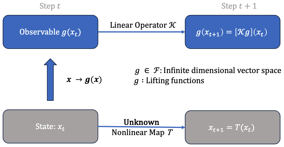
Figure 1 Sketch of the Koopman Operator Theory. Adapted from Shi et al. (2024).

Figure 2 Figure adapted from Wang et al. (2023), demonstrating uplifting.

Figure 3 Illustration of the DMD decomposition adapted from Erichson et al. (2016).

In this work we will focus on the amplitudes matrix and its role in explaining extreme events. The modes represent distinct spatial patterns that grow or decay with different frequency over time. The information about growth and decay is captured with the matrix evolution. Modes are ordered by their frequencies, with the first modes representing the dominant behaviours (Smith et al., 2005; Rowley et al., 2009b; Zhang et al., 2014). Each mode has a corresponding amplitude, that holds the information about the energy, i.e. the overall importance for the reconstruction.

2.1 Discretisation

In theory, we are interested in the dynamical system and its evolution:

$$\begin{array}{}\text{(3)}& {\displaystyle }{\displaystyle \frac{\mathrm{d}\mathit{x}}{\mathrm{d}t}}=f(\mathit{x},t;\mathit{\mu })\end{array}$$

with a high-dimensional state x(t)∈ℝ^m. The dynamics $f(\mathit{x},t;\mathit{\mu })$ is unknown, only the observations of the system state can be used to approximate the dynamics and predict the future state. In practice, we are analysing its discrete-time flow map

$$\begin{array}{}\text{(4)}& {\displaystyle }{\displaystyle }{\mathit{x}}_{k+\mathrm{1}}=F\left({\mathit{x}}_k\right)\end{array}$$

We search for the operator A that linearises the dynamics in form of:

$$\begin{array}{}\text{(5)}& {\displaystyle }{\displaystyle \frac{\mathrm{d}\mathit{x}}{\mathrm{d}t}}=\mathbf{A}\mathit{x}\end{array}$$

that has a closed-form solution:

$$\begin{array}{}\text{(6)}& {\displaystyle }{\displaystyle }\mathit{x}(t_{\mathrm{0}}+t)={\mathrm{e}}^{At}\mathit{x}\left(t_{\mathrm{0}}\right)\end{array}$$

The solution to this system may be expressed simply in terms of eigenvalues λ_j and eigenvectors ϕ_j of this discrete map A.

$$\begin{array}{}\text{(7)}& {\displaystyle }{\displaystyle }{x}_{k+\mathrm{1}}=\sum _{j=\mathrm{1}}^K{\mathit{\varphi }}_j{\mathit{\lambda }}_j^{k+\mathrm{1}}{b}_j\end{array}$$

where b_j∈ℂ, also called amplitude, contains the weights of the modes, the eigenvalues λ_j∈ℂ represent the temporal behaviour of the system and the eigenvectors ϕ_j∈ℂⁿ are the spatial modes. Equation (7) is a mathematical formulation of Fig. 3.

In theory, such a decomposition can be exact using finitely many modes, but in realistic flows this is rarely achievable. Instead, we aim to achieve the decomposition only approximately, by retaining a relatively small number of modes K.

2.2 Regression

The DMD method produces a low-rank decomposition of the matrix A by optimising the fit to the trajectory x_k

$$\begin{array}{}\text{(8)}& {\displaystyle }{\displaystyle }\Vert {\mathit{x}}_{k+\mathrm{1}}-\mathbf{A}{\mathit{x}}_k{\Vert }_{\mathrm{2}}\end{array}$$

where x_k and x_k+1 represent measurements taken at two consecutive timestamps, separated by time interval Δt.

This linearisation is valid only locally, as it represents the best local linear approximation of the system's time-evolving states (snapshots).

Since we want to minimise the error across all snapshots, we reshape all m snapshots into a high-dimensional column vectors and arrange them in two large matrices:

$$\begin{array}{}\text{(9)}& {\displaystyle }& {\displaystyle }\mathbf{X}=\left[\begin{array}{cccc}|& |& |& |\\ {\mathit{x}}_{\mathrm{1}}& {\mathit{x}}_{\mathrm{2}}& \mathrm{\dots }& {\mathit{x}}_{m-\mathrm{1}}\\ |& |& |& |\end{array}\right]\text{(10)}& {\displaystyle }& {\displaystyle }{\mathbf{X}}^{\prime }=\left[\begin{array}{cccc}|& |& |& |\\ {\mathit{x}}_{\mathrm{2}}& {\mathit{x}}_{\mathrm{3}}& \mathrm{\dots }& {\mathit{x}}_m\\ |& |& |& |\end{array}\right]\end{array}$$

and approximate the linear operator A that models the trajectory x(t) by formulating

$$\begin{array}{}\text{(11)}& {\displaystyle }{\displaystyle }{\mathbf{X}}^{\prime }\approx \mathbf{AX}\end{array}$$

Putting it all together we have the following definition.

Definition 2.

DMD

Suppose we have a dynamical system as in Eq. (3) and two sets of data (snapshots) X and X^′ as in Eqs. (9) and (10) so that $x_k^{\prime }=F\left(x_k\right)$ is the map in Eq. (4) corresponding to the map (Eq. 3) for time Δt. DMD computes the leading eigendecomposition of the best-fit linear operator A relating the data ${\mathbf{X}}^{\prime }\approx \mathbf{AX}$ (Tu et al., 2014).

Mathematically, the best-fit operator A is then defined as

$$\begin{array}{}\text{(12)}& {\displaystyle }{\displaystyle }\mathbf{A}=\arg \underset{\mathbf{A}}{min}\Vert {\mathbf{X}}^{\prime }-\mathbf{AX}\Vert ={\mathbf{X}}^{\prime }{\mathbf{X}}^{†}\end{array}$$

where † denotes the Moore–Penrose pseudo-inverse of a matrix.

The validity of the approximation in Eq. (12) is supported by the following theorem, which relies on the concept of linear consistency. But let us first introduce the definition of the linear consistency.

Definition 3.

Two matrices $\mathbf{X}\in {\mathbb{C}}^{n\times m}$ and ${\mathbf{X}}^{\prime }\in {\mathbb{C}}^{n\times m}$ are said to be linearly consistent if for every vector c∈ℂ^m, the condition Xc=0 implies ${\mathbf{X}}^{\prime }\mathit{c}=\mathrm{0}$.

Theorem 1.

Tu et al., 2014, Tu et al., 2014

If we define $\mathbf{A}\mathrm{=}{\mathbf{X}}^{\mathrm{\prime }}{\mathbf{X}}^{\mathrm{†}}$. Then ${\mathbf{X}}^{\mathrm{\prime }}\mathrm{=}\mathbf{AX}$ if and only if X^′ and X are linearly consistent.

We conclude that by inverting the usual focus of the method from modelling the system's average behaviour to emphasizing its exceptional dynamics. Additionally we refine the DMD algorithm accordingly so that extreme events can be modeled more accurately across several common metrics. Moreover, this approach enables the extraction of spatial patterns that contribute to the reconstruction of extremes, along with insights into their temporal evolution.

Even though in this work we focus on the diagnostic application, the method could be easily used for future state prediction. Diagnosing the evolution in time of extreme situations, one could detect reoccurring patterns and therefore predict the upcoming extremes. This extension is planned for the future work.

2.3 DMD Algorithm

As previously noted, the DMD algorithm identifies the best-fit linear operator that advances the system from one snapshot matrix to the next in time.

1. Compute the singular value decomposition of X (defined in 9), performing a low-rank truncation at the same time

   $$\begin{array}{}\text{(13)}& {\displaystyle }{\displaystyle }\mathbf{X}\approx \stackrel{\mathrm{̃}}{\mathbf{U}}\stackrel{\mathrm{̃}}{\mathbf{\Sigma }}{\stackrel{\mathrm{̃}}{\mathbf{V}}}^{*}\end{array}$$

   where * denotes the conjugate transpose, $\stackrel{\mathrm{̃}}{\mathbf{U}}\in {\mathbb{C}}^{n\times r}$, $\stackrel{\mathrm{̃}}{\mathbf{\Sigma }}\in {\mathbb{C}}^{r\times r}$, and $\stackrel{\mathrm{̃}}{\mathbf{V}}\in {\mathbb{C}}^{m\times r}$, and r≤m denotes either the exact or the approximate rank of the data matrix X

2. Project the full matrix A onto $\stackrel{\mathrm{̃}}{\mathbf{U}}$ and calculate $\stackrel{\mathrm{̃}}{\mathbf{A}}$

   $$\begin{array}{}\text{(14)}& {\displaystyle }{\displaystyle }\stackrel{\mathrm{̃}}{\mathbf{A}}={\stackrel{\mathrm{̃}}{\mathbf{U}}}^{*}\mathbf{A}\stackrel{\mathrm{̃}}{\mathbf{U}}={\stackrel{\mathrm{̃}}{\mathbf{U}}}^{*}{\mathbf{X}}^{\prime }\stackrel{\mathrm{̃}}{\mathbf{V}}{\stackrel{\mathrm{̃}}{\mathbf{\Sigma }}}^{-\mathrm{1}}\end{array}$$

3. Compute the eigenvalues λ_i (diagonal of matrix Λ) and eigenvectors w_i (columns of W) of $\stackrel{\mathrm{̃}}{\mathbf{A}}$. These eigenvalues and eigenvectors also correspond to the ones of the full matrix A.

   $$\begin{array}{}\text{(15)}& {\displaystyle }{\displaystyle }\stackrel{\mathrm{̃}}{\mathbf{A}}\mathit{W}=\mathit{W}\mathbf{\Lambda }\end{array}$$

4. The high-dimensional DMD modes Φ are reconstructed using the eigenvectors W and the time-shifted snapshot matrix X'. These DMD modes are eigenvectors of the high-dimensional matrix A corresponding to the eigenvalues in Λ.

   $$\begin{array}{}\text{(16)}& {\displaystyle }{\displaystyle }\mathbf{A}\mathbf{\Phi }=\mathbf{\Phi }\mathbf{\Lambda },\mathbf{\Phi }={\mathbf{X}}^{\prime }\mathbf{V}{\mathbf{\Sigma }}^{-\mathrm{1}}\mathit{W}\end{array}$$

5. Reconstruct the original signal

   $$\begin{array}{}\text{(17)}& {\displaystyle }{\displaystyle }{\mathbf{X}}_{\text{dmd}}=\mathbf{\Phi }{\mathrm{e}}^{\mathrm{\Omega }t}\mathit{b},\mathit{b}={\mathbf{\Phi }}^{†}{x}_{\mathrm{0}}\end{array}$$

The angular frequency ω_k associated with each eigenvalue λ_k is calculated ${\mathit{\omega }}_k=\frac{\ln \left({\mathit{\lambda }}_k\right)}{\mathrm{\Delta }t}b$, though alternative approaches exist. In our experiments, we will further explore these alternatives using optimisation techniques.

2.4 Optimisation

Our idea is closely related to the sparse DMD (Rudy et al., 2016), where the aim is to reconstruct the original signal using as few modes as possible. In other words, to find the solution that exhibits the best balance of accuracy and sparsity. This is implemented by adding a regularisation term γ in the regression step (Eq. 8), i.e. the L¹ penalty.

$$\begin{array}{}\text{(18)}& {\displaystyle }{\displaystyle }\underset{\mathit{b}}{min}J\left(\mathit{b}\right)+\mathit{\gamma }\sum _{i=\mathrm{1}}^r\left|b_i\right|\end{array}$$

where the objective function J(b) is defined by

$$\begin{array}{ll}{\displaystyle }J\left(\mathit{b}\right)& {\displaystyle }:={∥\mathbf{X}-\mathbf{\Phi }{\mathbf{D}}_b{\mathbf{V}}_{\mathit{\mu }}∥}_F\\ \text{(19)}& {\displaystyle }& {\displaystyle }=\sqrt{\sum _{i=\mathrm{1}}^m\sum _{j=\mathrm{1}}^n{\left(X_{ij}-{\mathrm{\Phi }}_{ij}{D}_{b_{ij}}{V}_{{\mathit{\mu }}_{ij}}\right)}^{\mathrm{2}}}\end{array}$$

where Φ denotes the matrix of DMD modes, as defined in Step 4 of the algorithm above, D_b=diag{b} has the amplitudes on the diagonal and V_μ is the Vandermonde matrix holding information about the angular frequency.

The goal is to control the amplitudes of the vector $\mathit{b}={\mathrm{\Phi }}^{†}{x}_o$. The vector b is used to reconstruct the system's time-evolution matrix and serves as the “starting point” for analysis. A central questions in sparse DMD is – Which modes best represent a system, and how can they be identified? This is a challenging problem. The proposed method aims to automate this process by reconstructing the data using as few DMD modes as possible. But the challenge remains – Which modes should be chosen?

In our DMD variation, we focus on identifying the modes that best reconstruct the system's extremes. To answer this question, we modify the objective function (Eq. 19) by adding an additional regularisation term that accounts for extreme events. We will call it a penalisation term, since it penalises the reconstructions in which the extremes are poorly represented.

$$\begin{array}{ll}{\displaystyle }& {\displaystyle }J\left(\mathit{b}\right)=\Vert \mathbf{X}-\mathbf{\Phi }{\mathbf{D}}_b{\mathbf{V}}_{\mathit{\mu }}\Vert =\sqrt{\sum _i\sum _j{\left(X_{ij}-{\mathrm{\Phi }}_{ij}{D}_{b_{ij}}{V}_{{\mathit{\mu }}_{ij}}\right)}^{\mathrm{2}}}\\ \text{(20)}& {\displaystyle }& {\displaystyle }+\underset{\text{penalisation term}}{\underbrace{\sqrt{\sum _{i\in M}\sum _{j\in M_i}(x_{ij}-{\mathit{\varphi }}_{ij}{D}_{b_{ij}}{V}_{{\mathit{\mu }}_{ij}}{)}^{\mathrm{2}}}}}.\end{array}$$

where M represents a set of temporal indices of extreme events and M_i is a set of spatial indices for a certain extreme event i. In Eq. (20), both the global and the extreme-set residuals are measured using the Frobenius norm. The second term represents a Frobenius-norm penalty applied to the subset of extreme observations.

The penalisation term reduces deviations from extreme events. Consequently, the objective function optimizes b to favour extraordinary modes, those responsible for detecting outliers, over average modes that capture typical behaviour.

3 Experiments

In our experiments, we utilise reanalysis data, as it represents the most accurate approximation to observations currently available. Although reanalyses are model-based reconstructions, they are constrained by observational data. Variables that are directly assimilated into the reanalysis forecast model tend to align more closely with real-world measurements.

For this study, we use the ERA5 reanalysis dataset (Hersbach and Dee, 2016), downloaded on a regular 0.25°×0.25° grid. Our spatial domain is restricted to Europe, spanning 70–36° N and 9° W–32° E, yielding a resolution of 17 892×31 224 grid points. The temporal coverage extends every day over 82 years, from 1940 to 2022. In the following experiments we focus on temperature anomaly in Europe. Although the method can be applied to any atmospheric variable.

The assumption is that the measurements are taken from the unknown dynamics and the research question is: Are there any coherent patterns of extremes from the hidden dynamics that can be discovered using DMD algorithm? To answer this question we implement the new variation of a Dynamic Mode Decomposition (DMD), called extreme DMD (defined in Eq. 20).

3.1 Analysis

In our experiments we compare two DMD variations, the normal and the extreme one, that includes an additional penalisation term. Having both reconstructions, we will analyse which of them performs better and which modes are significant in each of the reconstructions.

As previously mentioned, the significance information is encoded in the amplitude vector b. By comparing the two amplitude vectors, b_normal and b_extremes, we can determine which modes carry greater significance and which are less relevant when dealing with extreme events. Once these key modes are identified, the next step is to investigate their physical interpretation, which we leave for future work.

We extract the most important mode in this manner:

$$\begin{array}{}\text{(21)}& {\displaystyle }{\displaystyle }\text{most important mode index}=\arg max\mathit{\{}{\mathit{b}}_{\text{extreme}}-{\mathit{b}}_{\text{normal}}\mathit{\}}\end{array}$$

3.2 Persistent Extreme Event Detection and Validation

First let us define how we extract the persistent extreme events. In our test cases, we focus on heatwaves.

Heatwaves are prolonged periods of unusually hot weather, though their exact definitions vary across the literature (Xu et al., 2016). Typically, heatwaves are defined based on a combination of duration and high-temperature thresholds (Xu et al., 2016; Yin et al., 2022; Casati et al., 2013), often involving percentile-based approaches or specific indices, such as the ETCCDI indices (Vogel et al., 2020). Studies have shown that the choice of threshold influences projected changes in heatwave characteristics (Vogel et al., 2020), and this choice differs based on the regional climate (Perkins-Kirkpatrick and Gibson, 2017). Therefore, climate extremes such as heatwaves, are not only defined by peak values, they must also persist over a specific time period within a region. In our experiments, we define extreme heat events using a 95th percentile threshold and require a minimum duration of three consecutive timesteps above this level.

3.3 Local Maximum Detection

To identify extreme persistent events, we first detect a local maximum in a snapshot. We then compare this maximum to the following two snapshots to check if the maximum persists. The condition is that the maximum stays within the neighborhood (e.g. 5 pixels×5 pixels).

Let $\mathbf{D}(t,x,y)$ represent the data value at time t and spatial location (x,y). N represent the neighborhood size for initial detection.

For each time step t^*, identify $(x^{*},y^{*})$ as the location of a local maximum:

$${\displaystyle }\mathbf{D}(t^{*},x^{*},y^{*})=\underset{(i,j)\in N}{max}\mathbf{D}(t^{*},x^{*}+i,y^{*}+j)$$

3.4 Persistence Check Over Previous Time Step

For a local maximum $(x^{*},y^{*})$ at time t, check persistence over the previous two time steps, t−1 and t−2:

$$\begin{array}{ll}{\displaystyle }& {\displaystyle }\mathbf{D}(t-\mathrm{1},x^{*},y^{*})=\underset{(i,j)\in N}{max}\mathbf{D}(t-\mathrm{1},x^{*}+i,y^{*}+j)\\ {\displaystyle }& {\displaystyle }\mathbf{D}(t-\mathrm{2},x^{*},y^{*})=\underset{(i,j)\in N}{max}\mathbf{D}(t-\mathrm{2},x^{*}+i,y^{*}+j)\end{array}$$

If Local Maximum Detection and Persistence Check over Previous Time Steps are satisfied, only then $(t^{*},x^{*},y^{*})$ is considered a persistent maximum. The procedure to find minima works analogously. Importantly, the detection of extreme events is performed in the transformed modal space, rather than in the original data domain. This approach allows us to identify and isolate the specific dynamic modes that contribute most significantly to rare or extreme behaviour. As a result, it provides a more robust and interpretable basis for identifying outliers, compared to simply searching for large values in the raw data. Moreover, because the modal representation operates in a reduced-dimensional subspace, this approach is also computationally more efficient, making it well-suited for high-dimensional systems.

3.5 Extreme Dynamic Mode Decomposition

We modify the original DMD by adding the penalisation term, which is then solved by a convex optimization problem that balances the reconstruction error and extreme value penalisation. We are minimising the objective function defined in Eq. (20). We test the method across various ranks, but represent in the following section the results for rank 50.

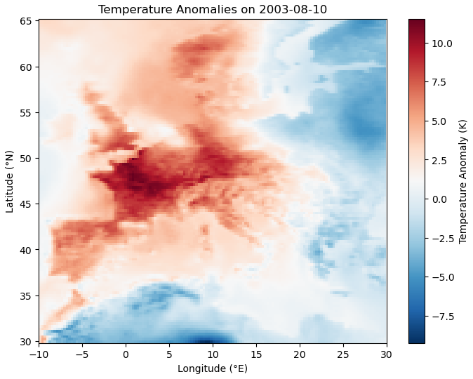
Figure 4 Heatwave of 2003: Spatial distribution of temperature anomalies (°C) over Europe on 3 August 2003.

3.6 Metrics

Reconstruction accuracy is evaluated using four distinct performance metrics:

• Mean squared error (MSE) measures the average squared difference between predicted values $\widehat{\mathit{y}}$ and the actual (true) values y

  $${\displaystyle }\text{MSE}={\displaystyle \frac{\mathrm{1}}{n}}\sum _{i=\mathrm{1}}^n{\left({\widehat{y}}_i-y_i\right)}^{\mathrm{2}}$$

• L-infinity norm (L_∞) (also called the maximum norm or supremum norm) of a vector measures the largest absolute value among its components. In other words, it captures the maximum magnitude of any single element in the vector.

  $${\displaystyle }\Vert \mathit{x}{\Vert }_{\mathrm{\infty }}=\underset{\mathrm{1}\le i\le n}{max}\left|x_i\right|$$

• The 10-norm is a specific case of the L_p-norm where p=10. It measures the “length” of a vector by taking the 10th root of the sum of the absolute values of the vector components raised to the 10th power. Higher-order norms (like the 10-norm) raise the absolute values to a high power before summing, which amplifies the effect of large components (i.e. outliers).

  $${\displaystyle }\Vert \mathit{x}{\Vert }_{\mathrm{10}}={\left(\sum _{i=\mathrm{1}}^n|x_i{|}^{\mathrm{10}}\right)}^{\frac{\mathrm{1}}{\mathrm{10}}}$$

• Structural Similarity Index Measure (SSIM) is a perceptual metric usually used to measure the similarity between two images (or signals) by comparing their luminance, contrast, and structural information. Unlike traditional error metrics (like MSE), SSIM aims to model the human visual system's sensitivity to changes in structural information, making it better suited for assessing perceived image quality.

  $${\displaystyle }\text{SSIM}(\mathit{x},\mathit{y})={\displaystyle \frac{(\mathrm{2}{\mathit{\mu }}_x{\mathit{\mu }}_y+C_{\mathrm{1}})(\mathrm{2}{\mathit{\sigma }}_{xy}+C_{\mathrm{2}})}{({\mathit{\mu }}_x^{\mathrm{2}}+{\mathit{\mu }}_y^{\mathrm{2}}+C_{\mathrm{1}})({\mathit{\sigma }}_x^{\mathrm{2}}+{\mathit{\sigma }}_y^{\mathrm{2}}+C_{\mathrm{2}})}}$$

  where:

  • μ_x and μ_y are the mean intensities of image patches x and y, respectively:

    $${\displaystyle }{\mathit{\mu }}_x={\displaystyle \frac{\mathrm{1}}{N}}\sum _{i=\mathrm{1}}^N{x}_i,{\mathit{\mu }}_y={\displaystyle \frac{\mathrm{1}}{N}}\sum _{i=\mathrm{1}}^N{y}_i$$

  • ${\mathit{\sigma }}_x^{\mathrm{2}}$ and ${\mathit{\sigma }}_y^{\mathrm{2}}$ are the variances of x and y, representing contrast:

    $$\begin{array}{ll}{\displaystyle }& {\displaystyle }{\mathit{\sigma }}_x^{\mathrm{2}}={\displaystyle \frac{\mathrm{1}}{N-\mathrm{1}}}\sum _{i=\mathrm{1}}^N(x_i-{\mathit{\mu }}_x{)}^{\mathrm{2}},\\ {\displaystyle }& {\displaystyle }{\mathit{\sigma }}_y^{\mathrm{2}}={\displaystyle \frac{\mathrm{1}}{N-\mathrm{1}}}\sum _{i=\mathrm{1}}^N(y_i-{\mathit{\mu }}_y{)}^{\mathrm{2}}\end{array}$$

  • σ_xy is the covariance between x and y, capturing structural similarity:

    $${\displaystyle }{\mathit{\sigma }}_{xy}={\displaystyle \frac{\mathrm{1}}{N-\mathrm{1}}}\sum _{i=\mathrm{1}}^N(x_i-{\mathit{\mu }}_x)(y_i-{\mathit{\mu }}_y)$$

  • C₁ and C₂ are small constants to stabilize the division, defined as:

    $${\displaystyle }{C}_{\mathrm{1}}=(K_{\mathrm{1}}L{)}^{\mathrm{2}},C_{\mathrm{2}}=(K_{\mathrm{2}}L{)}^{\mathrm{2}}$$

    where L is the dynamic range of pixel values (e.g. 255 for 8-bit images), and $K_{\mathrm{1}},K_{\mathrm{2}}\ll \mathrm{1}$.

3.7 Results

To facilitate interpretation of the following figures, we briefly recall the meaning of amplitudes and modes in the context of Dynamic Mode Decomposition (DMD). Each DMD mode represents a spatially coherent structure that evolves over time with a specific frequency and growth or decay rate. The associated amplitude quantifies the importance of that mode in reconstructing the observed system dynamics. In the proposed extreme DMD framework, the amplitude estimation is modified by a penalisation term that prioritises accurate reconstruction of extreme events. Therefore, differences in amplitudes between the Normal and extreme DMD indicate which spatiotemporal structures gain or lose influence when the method focuses on extremes rather than average behaviour. This interpretation underpins Figs. 5, 9, and 16, which highlight how the relative weighting of modes shifts in response to the extreme-event constraint.

3.7.1 Heatwave 2003

We now examine in detail the well-known heatwave that struck France in August 2003, one of the most extreme and widely studied heat events in recent history (García-Herrera et al., 2010). This heatwave was characterised by persistently high temperatures, leading to severe impacts on human health, agriculture, and infrastructure. The spatial extent of the heatwave during its peak in early to mid-August 2003 is illustrated in Fig. 4, highlighting the affected regions and the intensity of the temperature anomalies.

To clarify the methodology used in our experiments, in Fig. 5 we present a schematic analogue to Fig. 3, but constructed using our dataset corresponding to the 2003 heatwave. This illustration serves to provide a clearer understanding of the experimental setup and the specific data processing steps applied in our analysis.

Figure 5 Comparison of normal and extreme Dynamic Mode Decomposition (DMD) applied to the summer 2003 dataset. Both methods follow the same procedure as in Fig. 3 but differ in the amplitude estimation step, as shown by the two distinct amplitude matrices in the scheme. The temporal evolutions of the spatial patterns remains identical for both approaches (see Evolution plots in the scheme). The combination of modes, amplitudes, and evolution produces the reconstructed surface temperature anomalies shown in the rightmost panels: the upper panel corresponds to the Normal DMD reconstruction, and the lower panel to the extreme DMD. In extreme DMD, the amplitudes are optimised with an additional penalisation term that emphasizes the accurate reconstruction of extreme temperature values. Differences between the two reconstructions highlight how weighting extremes alters the spatial distribution and magnitude of the reconstructed anomalies, leading to an improved representation of the 2003 European heatwave.

Which reconstruction is better?

To show that the extreme DMD results indeed with better reconstruction, we show the following resulting reconstructions.

In Fig. 6, the left panel illustrates the reconstruction obtained using the standard (normal) Dynamic Mode Decomposition (DMD) without a penalisation term, while the middle panel presents the results of the modified extreme DMD approach, which incorporates a penalisation term. The rightmost panel displays the original data for reference. The dots in the plots denote extreme anomalies, with those in the middle panel highlighted in green when the reconstructed values closer match the original extreme events, as indicated by a lower mean squared error (MSE) and other metrics (see Figs. 7 and 8). We focus on August (indicated with the red rectangular in Fig. 6.), the peak of the heatwave period.

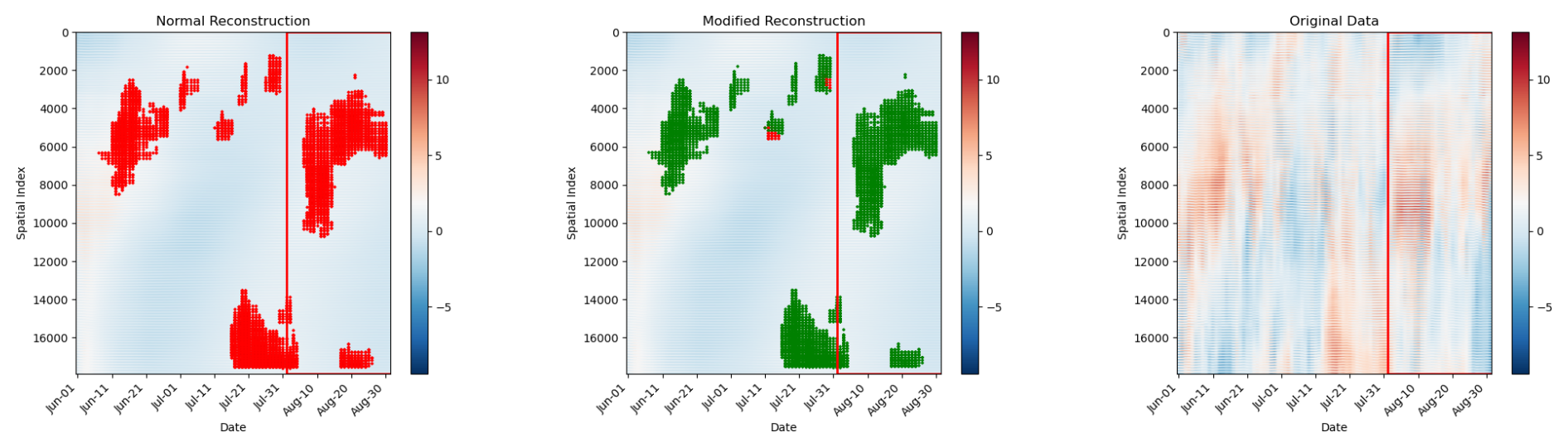
Figure 6 Comparison of reconstructions for the 2003 heatwave. Each plot shows time (x axis) vs. space (y axis), corresponding to the flattened snapshots illustrated in Fig. 3. Red and green markers denote the occurrence of extreme events. (a) Normal DMD reconstruction, (b) extreme DMD reconstruction, where green highlights indicate extremes better captured (lower MSE) compared to the normal DMD case, and (c) original anomaly field serving as reference. The red frame marks the August period, when most extreme events occurred. All reconstructions follow the scheme shown in Fig. 5.

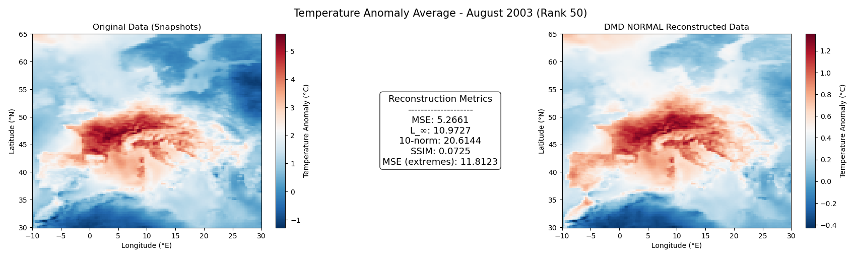
Figure 7 The left panel shows the average temperature anomaly in August based on the original ERA5 data (reference), while the right panel shows the corresponding reconstruction using the normal DMD method. The middle panel presents various metrics that evaluate the quality of the reconstruction.

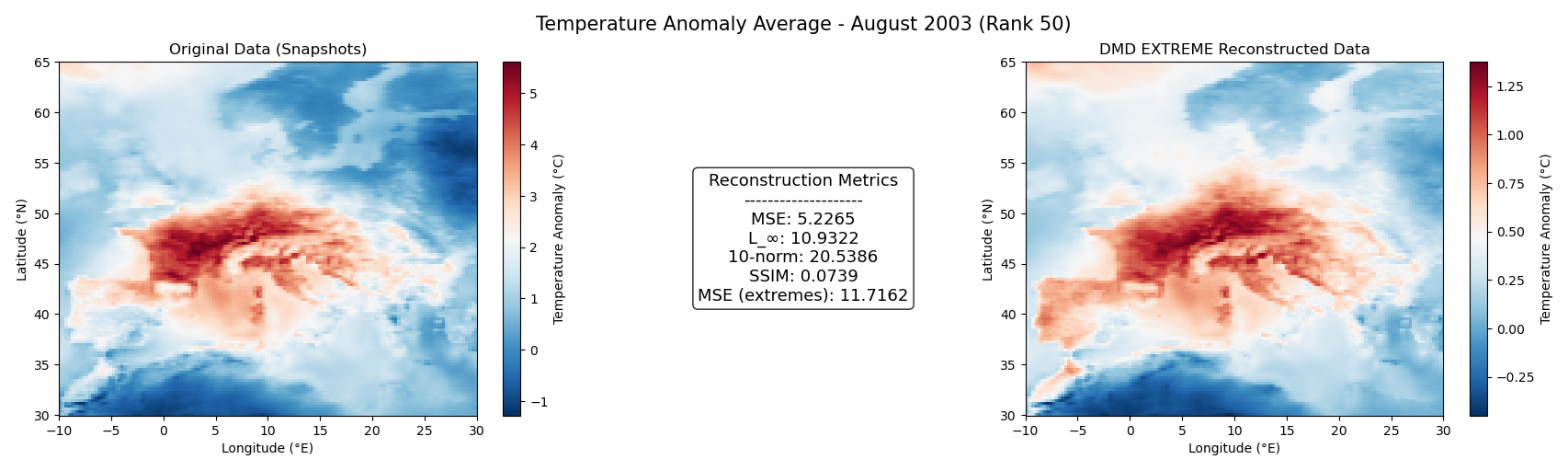
Figure 8 The left panel shows the average temperature anomaly in August based on the original ERA5 data (reference), while the right panel shows the corresponding reconstruction using the novel extreme DMD method. The middle panel presents various metrics that evaluate the quality of the reconstruction.

By analysing and comparing various metrics presented in Figs. 7 and 8, we observe that the differences are subtle but systematic and aligned with our goal of capturing extremes. The proposed method – extreme DMD (results in Fig. 8) – offers a more accurate representation of extreme values.

Statistical comparison between the extreme DMD and standard DMD reconstructions at extreme spatiotemporal points (MSE (extremes)) showed a significant improvement for the extreme DMD (t=90.150, p<0.001). The effect size (Cohen's d=0.558) indicates a moderate enhancement, with a 95 % bootstrap confidence interval for the mean MSE reduction of [0.094103,0.098255]. These results confirm the superior reconstruction accuracy of the extreme DMD method during extreme events.

Which modes have more significance and which less in each of the reconstructions?

After running two different optimization problems: without penalising the extreme events (minimising Eq. 19) and once with penalising the extreme events (minimising Eq. 20), we compare the resulting optimal solutions – the amplitudes b's – and we search for the biggest absolute difference.

In this experiment (with rank 50), the most important mode related to extreme events, defined by the highest amplitude difference, is mode 35 (see Fig. 9). We extract this mode along with its temporal dynamics and present them in Fig. 10.

Figure 9 Comparison of mode amplitudes between the normal and extreme Dynamic Mode Decomposition (DMD) for the 2003 heatwave event. Each bar represents the amplitude of a single mode, quantifying its contribution to the reconstructed temperature field. The largest absolute amplitude difference between the two methods is highlighted in red, the second largest in orange, and the third in purple. Additional modes marked with red circles indicate smaller but notable deviations, where the extreme DMD assigns higher amplitude values than the normal DMD. These highlighted differences identify which modes are most affected by the extreme-event penalisation term and thus contribute more strongly to the reconstruction of extreme temperature anomalies.

Figure 10 Spatial pattern and the dynamics of the 1st most important mode.

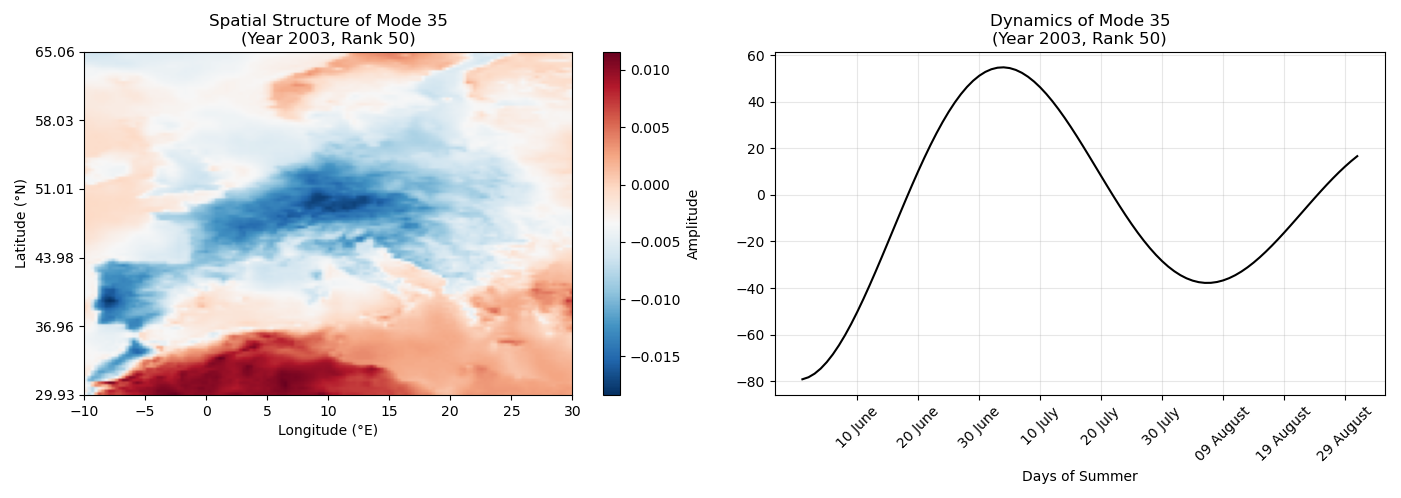
Figure 10 illustrates that the pronounced anomaly contrast between Europe and northern Africa is more influential in shaping the average behaviour of temperature anomalies than the extreme events. The temporal evolution of this mode reaches its maximum influence in late June, as evident on the right side of the panel.

A spatial pattern exhibiting higher amplitude values in the extreme DMD reconstruction (unlike the others) shown in Fig. 11 suggests that the pronounced contrast in anomalies between Northeastern and Western Europe played one of the key role in driving the 2003 heatwave in France.

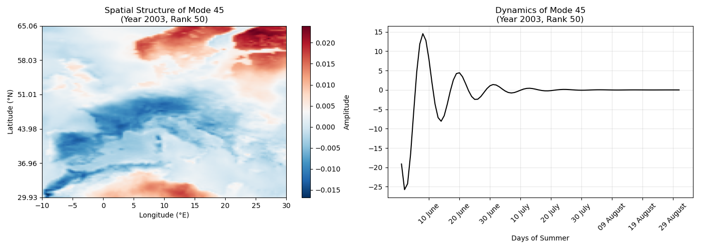
Figure 11 Spatial pattern and dynamics of the mode 45 – mode exhibiting the greatest increase in optimised b (b_extreme) value relative to the normal b (b_normal) value (red circles in the Fig. 9).

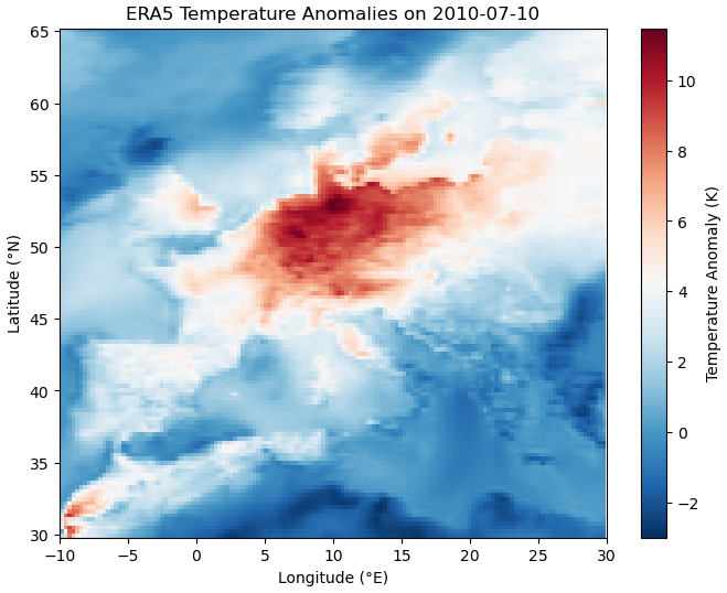
Figure 12 Heatwave of 2010: Spatial distribution of temperature anomalies (°C) over Europe on 10 July 2010.

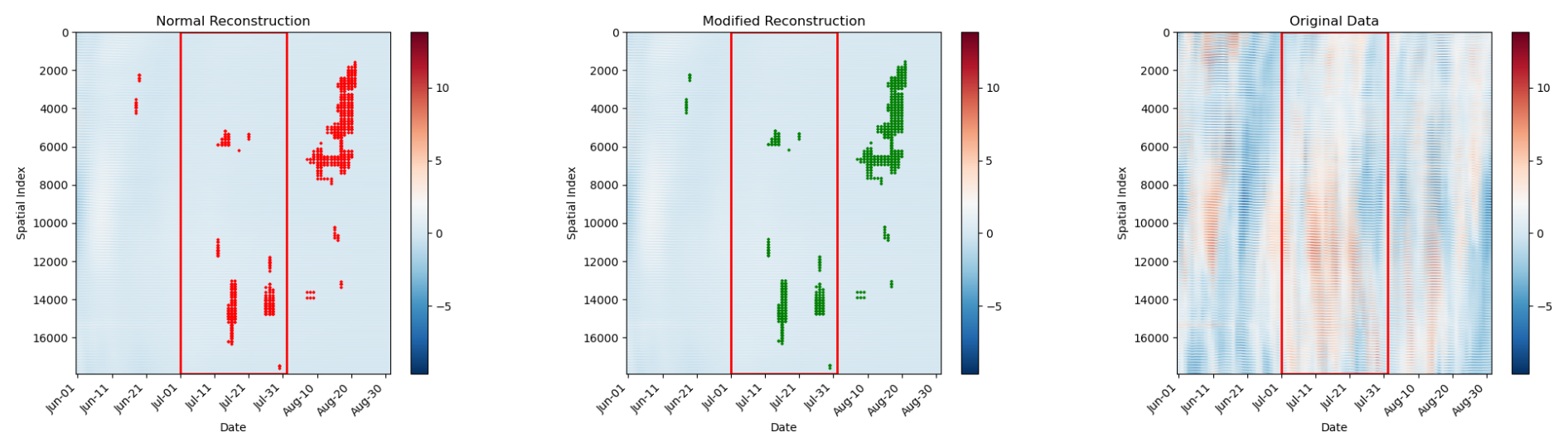
Figure 13 Comparison of reconstructions for the 2010 heatwave. Each plot shows time (x axis) vs. space (y axis), corresponding to the flattened snapshots illustrated in Fig. 3. Red and green markers indicate the occurrence of extreme events. (a) Normal DMD reconstruction, (b) extreme DMD reconstruction, where green highlights indicate extremes better captured (lower MSE) compared to the normal DMD, and (c) original anomaly field as reference. The red frame marks the July period, when extreme events had the greatest impact.

3.7.2 Heatwave 2010

In Northern Germany, the heatwave in 2010 led to unusually high temperatures, with several regions experiencing prolonged periods above 35 °C (Barriopedro et al., 2011). The extreme heat contributed to drought conditions, affecting agriculture and low water levels in rivers such as the Elbe and Weser. Additionally, urban areas like Hamburg and Bremen recorded significantly above-average temperatures, causing discomfort and increasing energy demand for cooling. While the heatwave in Germany was not as intense as in Russia, it still had noticeable impacts on public health and infrastructure. Here, we present the temperature anomalies that affected Northern Europe in mid-July.

Which reconstruction is better?

To evaluate the results, we conduct the reconstruction comparison using the same approach as in the previous experiment for the 2003 heatwave. The plotted dots denote extreme anomalies, with green highlighting regions where the reconstruction aligns more closely with the original extreme values.

The results clearly demonstrate that the extreme DMD approach leads to a more accurate representation of extreme temperature anomalies. This improvement is quantified by a lower mean squared error (MSE), both for the overall reconstruction and specifically for the extreme anomalies. Notably, all major extreme values observed during the 2010 heatwave are better captured using the modified DMD approach, further reinforcing the effectiveness of incorporating penalisation in detecting and reconstructing extreme climate events. This behaviour is further quantified by other metrics shown in Figs. 14 and 15.

Figure 14 The left panel shows the average temperature anomaly in July based on the original ERA5 data (reference), while the right panel shows the corresponding reconstruction using the normal DMD method. The middle panel presents various metrics that evaluate the quality of the reconstruction.

Figure 15 The left panel shows the average temperature anomaly in July based on the original ERA5 data (reference), while the right panel shows the corresponding reconstruction using the novel extreme DMD method. The middle panel presents various metrics that evaluate the quality of the reconstruction.

Consistent with earlier findings, the differences in performance metrics presented in Figs. 14 and 15 are subtle yet systematic, and once again align with our objective of enhancing the representation of extreme events. The proposed method – extreme DMD (results shown in Fig. 15) – demonstrates improved accuracy in capturing extreme values.

Statistical evaluation further supports this improvement. A paired t test revealed a highly significant difference between the two reconstructions (t=29.82, p<0.001), with a large effect size (Cohen's d=0.83). The 95 % bootstrap confidence interval for the mean improvement ranged from 0.076 to 0.087, confirming that extreme DMD consistently outperforms the standard DMD approach in reproducing extreme temperature anomalies.

Which modes have more significance and which less in each of the reconstructions?

Again we compare the amplitude vectors b's which are optimisation results with the penalisation term (minimising Eq. 20) and without (minimising Eq. 19).

The most important mode (spatial pattern) and its corresponding temporal dynamics are presented. This mode is identified based on the largest amplitude difference, as shown in Fig. 16.

Figure 16 Comparison of mode amplitudes between the normal and extreme Dynamic Mode Decomposition (DMD) for the 2010 heatwave event. Each bar represents the amplitude of a mode, indicating its relative contribution to the reconstructed temperature field. The largest absolute amplitude difference between the two methods is highlighted in red, the second largest in orange, and the third in purple. These highlighted modes exhibit the strongest response to the inclusion of the extreme-event penalisation term, showing how the extreme DMD reweights the contribution of certain spatiotemporal structures to better capture high-magnitude temperature anomalies. Overall, the differences emphasise which modes gain importance when the reconstruction focuses on extremes rather than average system behaviour.

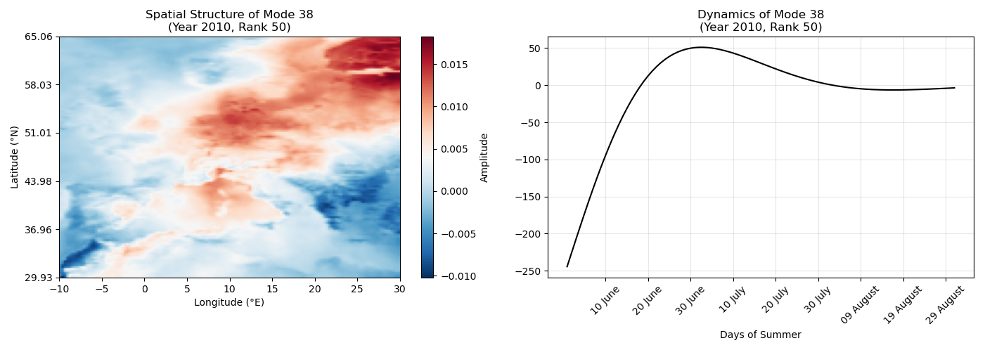
The spatial pattern of this particular 1st most important mode reveals the spatial pattern that strongly influences the average summer in Europe, but was less pronounced during the 2010 heatwave. It suggests a particularly strong and long-lasting blocking pattern developed over Russia. This blocking event was particularly intense from early July to mid-August 2010 (Schaller et al., 2018), which is also confirmed by the dynamics showed on the right panel. The dynamics exhibited a marked increase at the beginning of summer (during June), followed by a relatively stable period with minimal oscillations throughout the remaining summer months.

Figure 18 shows the spatial pattern and temporal dynamics of the mode exhibiting the largest increase in optimised b (b_extreme) compared to the normal b (b_normal). This mode captures a pronounced anomaly contrast between Eastern Europe (extending into Western Asia) and the rest of the continent, suggesting a strong contribution to the 2010 heatwave. The associated dynamics reveal that this spatial pattern was most prominent at the beginning of the summer and gradually weakened as the season progressed.

Figure 17 Spatial pattern and the dynamics of the 1st most important mode.

4 Discussion

Until now, reduced-order techniques have primarily focused on capturing the average behaviour of a system by filtering out noise and retaining only the dominant modes. In contrast, we challenge this perspective by asking whether the method can be reversed to reveal the exceptional modes that characterize extreme events. Hence, we introduce a theoretical framework aimed at identifying outliers together with their associated spatiotemporal modes. This allows for a deeper understanding of the underlying dynamics and helps to uncover the drivers of extreme events within the climate system. The results presented here demonstrate that the proposed framework more effectively identifies outliers compared to the standard DMD method.

The main contribution of this work is a theoretical framework specifically designed to better detect outliers and approximate extreme – rather than average – behaviour.

Our experiments clearly show that the original signal contains significantly more noise than the reconstructed fields, particularly as we move further forward in time. This is consistent with strong performance of the Koopman operator on a local scale. However, the primary objective of these experiments was to assess the effectiveness of the proposed DMD variation in accurately capturing extreme anomalies.

Given the current excitement surrounding large language models (LLMs), it is worth to mention that LLM architecture is equivalent to the Koopman operator-based architecture. However Koopman Operator Theory offers a robust framework for unsupervised learning using small amount of data, facilitating self-supervised learning of generative models that aligns more closely with human learning theories compared to some machine learning approaches (Mezić, 2023). Furthermore, by looking at significant modes (as in Figs. 10 and 11, etc.) a physical understanding of driving patterns can be derived from DMD.

Figure 18 Spatial pattern and dynamics of the mode exhibiting the greatest increase in optimised b (b_extreme) value relative to the Normal b (b_normal) value (red circle in the Fig. 16).

To validate the robustness of our event definition, we conducted a sensitivity analysis using 90th, 95th, and 99th percentile thresholds for extreme temperature anomalies. The resulting spatial modes and their temporal evolution remained consistent across all thresholds, indicating that the extreme DMD framework is largely insensitive to the specific percentile used. This robustness supports the rationality of the selection criterion and confirms that the essential spatiotemporal dynamics of extremes are well captured within the identified modal space, even when events outside this subspace are considered.

One of the central concern of every reduced order technique is the decision of the number of modes needed to represent the original signal. It is always a trade off between the accuracy and the complexity. Naturally, the higher the number of modes used in the reconstruction, the better the reconstruction will be (in terms of lower mean square error). However, increasing the complexity – represented by the rank parameter in our DMD algorithm – risks introducing noise into the reconstruction while also significantly raising computational cost. Our method was tested across various ranks, with all experiments consistently showing improvements when the penalisation term was added. So, we can safely claim that the method is robust with respect to the selection of the size of the rank. Unlike most of the other statistical approaches, we use rank as the only parameter, which allows for better interpretation of the model and more effective extraction of spatiotemporal patterns related to climate extremes. Sensitivity analysis of rank choice is provided in the Appendix.

The proposed framework is designed to be applicable to a broad range of climate extremes. While the current experiments have focused on temperature anomalies, specifically heatwave events, the approach can be readily extended to other types of extremes such as cold spells, heavy precipitation.

Although the present study focuses on reconstructing extreme events, the extreme DMD framework could be extended to short-term forecasting. Once the spatiotemporal modes and amplitudes are identified, the system's future state can be projected by evolving the amplitudes according to the DMD linear dynamics. This approach could provide early-warning indicators by highlighting modes associated with high-amplitude extremes.

Practical challenges must be considered. The linear evolution assumption may limit predictive skill for highly nonlinear events, and mode selection or amplitude initialization requires careful calibration when applying the model to new conditions or different climate regimes. Real-time forecasting would also require near-real-time data assimilation. Nevertheless, integrating extreme DMD with ensemble methods or existing forecasting frameworks has the potential to enhance the prediction of extreme climate events, supporting risk assessment and mitigation strategies.

The present study primarily focuses on the methodological extension of DMD for capturing extreme events. Although the extracted modes are dynamically coherent, a detailed physical interpretation–such as linking these modes to specific circulation anomalies, blocking events, or teleconnection patterns–remains an open question. Previous studies (e.g. Froyland et al., 2021; Chowdary et al., 2023; Zhang et al., 2025) have demonstrated that DMD and related Koopman-based approaches can reveal physically interpretable climate structures, suggesting that similar connections may be established here. Investigating such relationships will be an important avenue for future work aimed at bridging data-driven decomposition with atmospheric dynamics.

5 Conclusions

This work introduces a novel Dynamic Mode Decomposition (DMD) variation tailored to improve the reconstruction of extreme events and to extract spatiotemporal patterns (modes) specifically relevant to such extremes. Our study makes three key contributions:

• a.

  Regularisation design: We incorporate an extreme-event penalisation term into the DMD objective function, allowing the reconstruction to emphasize rare but important events.

• b.

  Mode selection: The framework enables automated identification of modes most relevant to extremes, providing a systematic approach to isolate the spatial patterns driving extreme behaviour.

• c.

  Climate science insight: Applying this method to European heatwaves reveals coherent spatiotemporal structures and the distinct impacts of anthropogenic emissions on extreme events, improving understanding of climate variability.

By shifting the focus from modelling average system behaviour to emphasising exceptional dynamics, the method achieves more accurate reconstruction of extremes and enables the extraction of interpretable spatial patterns and their temporal evolution. Heatwaves were chosen as a representative example to demonstrate the methodology; however, the approach is not limited to heat extremes. Extending the framework to other types of climate extremes – such as cold spells or heavy precipitation – remains an important direction for future work. Although our analysis focuses on diagnostic applications, the framework could also be adapted for short-term forecasting, offering a potential tool for anticipating extreme events based on emerging spatiotemporal patterns.

Appendix A: Sensitivity to Rank Selection

To assess the robustness of the proposed method with respect to the selected truncation rank (SVD Rank), we evaluated reconstruction performance across a range of ranks commonly used in DMD analyses. Figure A1 shows the mean squared reconstruction error at extreme spatiotemporal points (MSE (extremes)) for both the standard DMD and the extreme DMD. Across all tested rank values, extreme DMD consistently achieved lower error than standard DMD. This demonstrates that the improved representation of extreme events is not dependent on a particular choice of rank and holds over a broad range of truncations. In addition, the plot shows that increasing the rank leads to systematically lower MSE values for both methods, with the gap between the two approaches widening slightly at higher ranks. This indicates that our method benefits from richer modal information and that the identification of extreme – relevant modes and the resulting reconstruction improvements are stable – and even strengthened – when the model order increases.

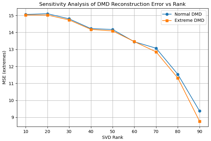
Figure A1 Sensitivity of extreme-event reconstruction to truncation rank. Across all tested SVD ranks, extreme DMD yields lower (MSE extremes) than standard DMD, indicating robustness to model order selection.