Fractal attractor of the deep convection cycle in the northwest Mediterranean Sea

Deep convection in the Gulf of Lion is an important ocean mixing process in the western Mediterranean Sea caused by large cooling fluxes at the sea surface. It aids the Mediterranean thermohaline circulation, and promotes phytoplankton blooming. This work investigates the three different periods of the process: preconditioning, deep convecting, and restratification, through the lens of fractal attractor analysis with the local correlation dimension. From the analysis it was determined that the preconditioning period is most predictable period, with a local correlation dimension of 10 to 20, followed by the deep convecting period, with a local correlation dimension of 15 to 50. However, the deep convecting period can also exhibit random-process-like behavior with local correlation dimensions growing exceedingly high in April and May. The least predictable period was the restratification period, with typical local correlation dimensions of 35 to 90 near the end of restratification.

1 Introduction

Geophysical flows are perhaps the most classical example of chaotic behavior. This result is well captured and demonstrated by the work of Lorenz (1963). In the ocean, typically this behavior is captured through the intrinsic ocean variability computed through ensemble modelling (Sérazin et al., 2015), where it strongly influences the smaller spatial scales (length scales less than 6°) and time scales (less than 18 months), but also influences the larger scales (Sérazin et al., 2015; Grégorio et al., 2015).

Open ocean deep convection occurs semi-frequently in the Gulf of Lion, in the northwest Mediterranean Sea (Somot et al., 2016). In this region, the process is driven by strong air-sea heat fluxes that cool the water surface over time until the vertical density gradient is eroded, homogenizing the temperature and salinity within the column, which allows it to convect. The Mistral and Tramontane winds, along with seasonal changes in the atmosphere over the gulf, create these fluxes (Keller et al., 2022, 2024). The process itself occurs primarily in three periods: the preconditioning period, deep convecting period, and restratification period (Marshall and Schott, 1999; The Lab Sea Group, 1998). The preconditioning period starts near the end of summer and progresses with the gentle deepening of the mixed layer until roughly February, where if enough cooling at the sea surface has occurred, the deep convection period is triggered. Deep convection can last for a few days to a few weeks, before the horizontal gradients of less dense fluids surrounding the deep convection patch overcome the vertical mixing and restratify the vertical column (Madec et al., 1991). This last step is called the restratification period, and lasts until the beginning of summer.

Deep convection in the Gulf of Lion generates the Western Mediterranean Deep Water (WMDW) from its intense vertical mixing of cooled Atlantic Water (AW) and Eastern Intermediate Water (EIW), which aids the general thermohaline circulation of the Mediterranean Sea (Robinson et al., 2001). After its formation, the WMDW spreads out along the bottom of the western Mediterranean Sea basin (MEDOC Group, 1970), flowing towards the Balearic Sea (Send and Testor, 2017), southward to the southern Algerian Basin within eddies (Beuvier et al., 2012; Testor and Gascard, 2003), and out to the Atlantic Ocean through the Strait of Gibraltar. The vertical mixing also promotes oxygen and nutrient distribution along the vertical column, resulting in large phytoplankton blooms proceeding deep convection events (Coppola et al., 2017; Severin et al., 2017). As a consequence of the process's impact on other major phenomena, much effort has been devoted to understanding the deep convection process, and in particular the deep convection period of the three aforementioned periods.

Deep convection in the Gulf of Lion has been studied through the lens of chaotic behavior before and has shown to be influenced by the intrinsic variability of the ocean, which contributes around 15 % to 30 % of the total temporal variability, depending on the system parameter (Waldman et al., 2018). For example, the resulting dense water formation of WMDW is known to be significantly affected by the initial conditions when modelled (Léger et al., 2016) and shows considerable spread in post deep convection attributes. Other studies have noted the significant spread of the deep convection mixed layer depth with ensemble modelling, particularly for the winter of 2012/2013 (Waldman et al., 2017a, b). However, these works focus mainly on the deep convection period in particular, and less so on the other two periods. The focus is kept on the deep convection period due to previously mentioned motivation and because the convection itself is typically the most difficult part of the process to recreate via modelling. Therefore, the other two periods haven't had as much attention devoted to them.

This paper further dives into the chaotic nature of deep convection in the Gulf of Lion, but includes investigating the preconditioning and restratification periods. The method used here doesn't require computationally intensive ensemble modelling and perhaps more directly measures the chaotic behavior of the system at hand. The local dimensionality of the deep convection system, used in this work, is computed from a high spatial resolution reanalysis that covers from 1987 to 2022 (Escudier et al., 2021), which can be used to describe the chaotic variability, therefore the predictability, of each system state. The method does so by measuring the fractal dimension of the system's dynamic, fractal attractor for each time step (Lucarini et al., 2012; Faranda et al., 2017). By using this technique, we can determine the predictability of each time step of deep convection in the Gulf of Lion, and describe the resulting predictability of the three open ocean convection periods. In the methodology section that follows (Sect. 2), the local correlation dimension is described (the metric of local dimensionality) and the steps taken to revise the reanalysis dataset of the Gulf of Lion to be more representative of the mixed layer depth (MLD) found in other studies (e.g. in Somot et al., 2016). This is followed by the results and discussion sections (Sects. 3 and 4), where the calculated local dimensions are presented and the predictability of the three different deep convection periods are discussed, respectively. Concluding remarks follow in Sect. 5.

2 Methodology and Data

2.1 Local Correlation Dimension and Local Dimensionality

A method to understand the fractal attractor of a system from observations is to determine its local correlation dimension (also called pointwise dimension), d, through Extreme Value Theory (EVT) (Lucarini et al., 2012; Faranda et al., 2017). d is a flavor of the fractal dimension measuring techniques (Grassberger, 1983; Grassberger and Procaccia, 1983; Lopes and Betrouni, 2009; Strogatz, 2014) and here it effectively represents the local density of the system's states on its attractor (the recurrence of the system to that location). It also measures the number of dimensions needed to describe the current state (or the attractor's local geometric dimension) and implies the number of next states the system could evolve into ($\mathrm{0}<d<\mathrm{\infty }$), which effectively defines each state's predictability (Aurell et al., 1997; Boffetta et al., 1998). It can be computed by first determining the natural log of the distances between a particular system state, ξ, and all other states, x(t≠t_i) (therefore ξ=x(t_i)):

$$\begin{array}{}\text{(1)}& g_{\mathrm{1}}=-\ln \left(\mathrm{dist}\right(\mathit{\xi },\mathit{x}(t\ne t_i)\left)\right)\end{array}$$

This is the first case observable in Lucarini et al. (2012). Then take an arbitrary threshold, T, to find the set of distances, z, that exceed this threshold (i.e. $z=g_{\mathrm{1}}-T$). If T is sufficiently large (e.g. the 98th percentile of g₁) and z primarily captures the extreme values of g₁, then the distribution of z can be analyzed with EVT. In this case, the distribution of z follows that of the Generalized Pareto Distribution (GPD). g₁ is computed per each time step (i.e. per each system state), to provide a z distribution for each system state.

With this particular definition of g₁, the distribution of z actually collapses onto a scaled exponential distribution, which is a simplified GPD. From this result, Lucarini et al. (2012), and Faranda et al. (2017), d is the reciprocal of the mean value of z's distribution. This means we have an estimation of the system's attractor's local correlation dimension for each provided system state, and therefore time step. Hereafter, d will be referred to as the local dimensionality of the given system state, which is consistent with other works using this method (e.g. Faranda et al., 2017).

This methodology should be insensitive to both the choice of distance function, dist, and threshold, T. However, in application, both can have an impact on the final results (Faranda et al., 2017). In this study, the Euclidean distance is used as the distance function and the 98th percentile of g₁ is taken as the threshold. Both have been used in prior works with this method (Faranda et al., 2017).

The benefit of using this methodology is only one simulation run is required to investigate the predictability and chaos of the ocean, whereas with ensemble modelling, by definition, requires multiple simulation runs. However, there is a trade-off: this methodology captures the chaotic behavior for each system state (time step) but loses the spatial information, as it is swallowed up into the distance calculation in Eq. (1). This is retained in ensemble modelling, such as seen in Sérazin et al. (2015) and Waldman et al. (2018).

2.2 System State Variable: Mixed Layer Depth

For this study, the mixed layer depth (MLD) will be taken as the representative system state of deep convection in the Gulf of Lion. This metric is the traditional metric used to follow deep convection, as it directly provides the depth from the surface to the vertical extent of the water that is homogenized in terms of temperature and salinity (Somot et al., 2016). Local dimensionality could be computed directly with the 3D fields of temperature and salinity. However, this is more computationally expensive than using the 2D mixed layer depth field, and would be providing the same information for this study case.

The MLD used for this study is from the high resolution reanalysis of the Mediterranean Sea performed by the Centro Euro-Mediterraneo sui Cambiamenti Climatici (CMCC) (Escudier et al., 2021) with the Nucleus for European Modelling of the Ocean model (NEMO; https://www.nemo-ocean.eu, last access: 23 April 2025) (Madec and the NEMO team, 2008). The reanalysis covers the years of 1987 to 2022 with a daily temporal resolution. It has a horizontal resolution of about 4 to 5 km ($\mathrm{1}/\mathrm{24}$°), with 141 unevenly spaced, vertical levels. It was accessed via the Copernicus Marine Service Data Store (CMEMS; https://doi.org/10.25423/CMCC/MEDSEA_MULTIYEAR_PHY_006_004_E3R1, Escudier et al., 2020) and is the highest resolution reanalysis of the Mediterranean Sea available on CMEMS.

For this work, only the values within the bounds of −0.4° E (the coast to the east) to 9.5° E and 38.8 to 44.5° N (the coast to the north) will be considered, as this area wholly captures the northwestern Mediterranean Sea and the Gulf of Lion within it (this area is shown in Fig. 1). The resulting states, x(t), are then a 238 by 137 by t (lon. by lat. by time) spatial, temporal grid of the MLD. The Euclidean distance, as the distance function used in this work in Eq. (1), is calculated by flattening the spatial dimensions of ξ and x(t≠t_i) each into a 1D vector during the comparison (recall that the z distribution is calculated per each time step, therefore the temporal dimension is not flattened).

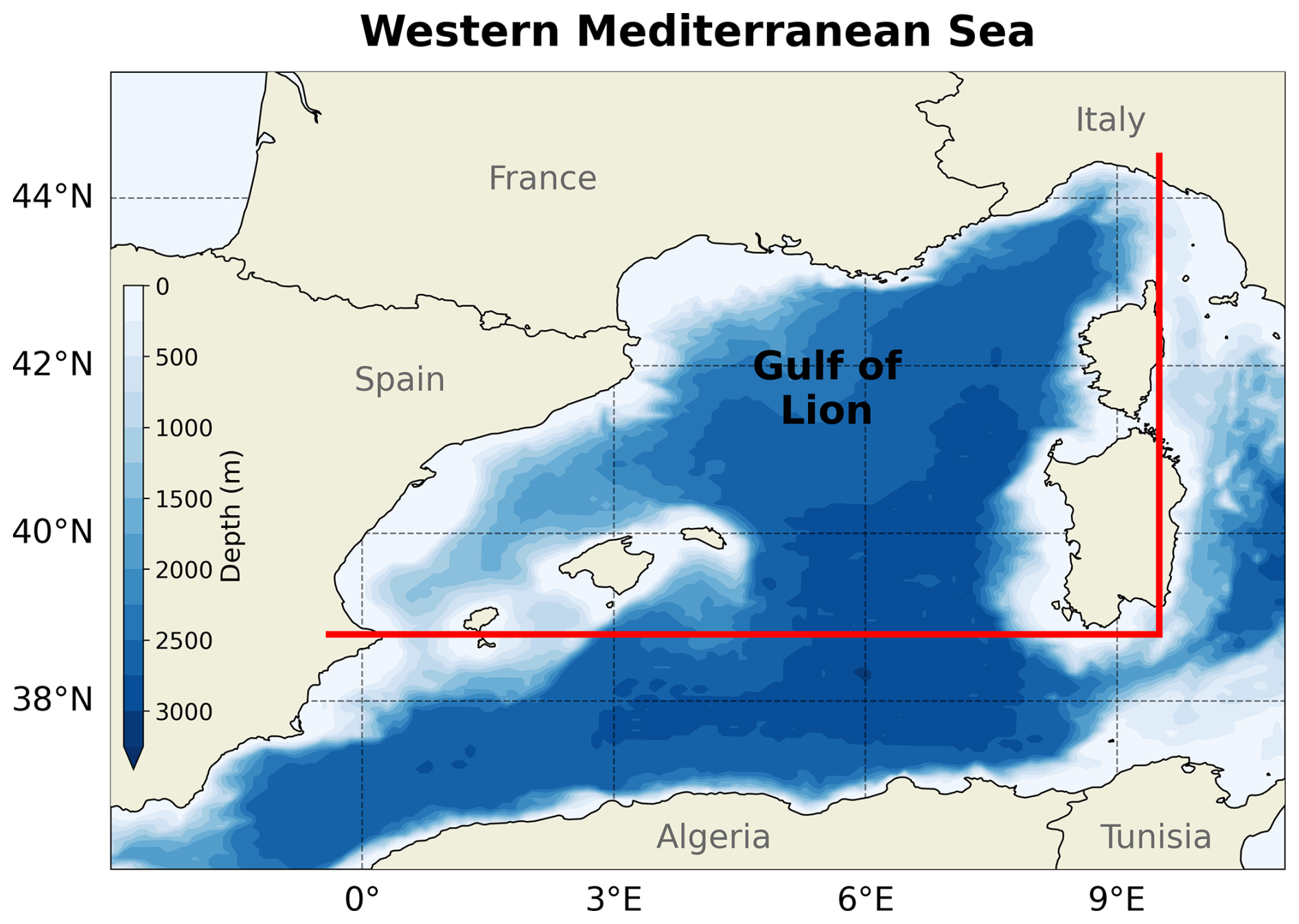
Figure 1 Study area with bathymetry: the Gulf of Lion in the northwestern Mediterranean Sea. The red lines mark the boundary of the area of interest (the eastern coast or −0.4 to 9.5° E and 38.8° N to the northern coast or 44.5° N).

2.3 Argo Mixed Layer Depths

To cross check the validity of the reanalysis MLD, MLD calculations from Argo float profiles are used. The MLD calculations were performed by Holte et al. (2017) and provided at https://mixedlayer.ucsd.edu (last access: 22 February 2023). 17 935 MLD calculation points were used from this dataset, which covers this dataset's entire temporal range for the MLD spatial domain in Fig. 1. The MLD was determined via a density based algorithm (Holte and Talley, 2009) (also see http://mixedlayer.ucsd.edu for more details, last access: 22 February 2023). The algorithm they use is fairly in-depth and is only briefly presented here from their work: “the algorithm models the profile's general shape, calculates a suite of possible MLD values, and then looks for groupings and patterns within the possible MLDs to select the final MLD estimate for each profile” (Holte and Talley, 2009).

2.4 Modified Mixed Layer Depths

When comparing the Argo determined MLDs and reanalysis MLDs, the reanalysis seemingly overestimates the occurrence of deep convection in the Gulf of Lion (see Fig. 3a). The MLD maxima (calculated per month over the spatial domain) of the Argo data tends to remain less than 500 m for most years of its availability. Conversely, nearly all years of the reanalysis show MLD maxima (calculated per day over the spatial domain) below 1000 m. While this could be due to the more complete spatial coverage of the MLD with the reanalysis data, as the Argo data is in the form of a few points per day, the Q-Q plot comparing the two show that they are comparable on the deeper end (see Fig. 2). In fact, the Argo dataset appears to have more, slightly deeper MLDs after quantile 0.2 up to 0.9. Below 0.2, the reanalysis quantiles are effectively flat with respect to the Argo quantiles, as the first grid depth for the model is at 5.87 m, acting as a floor for the shallowest MLDs in the dataset. The Argo dataset does not have this MLD value floor.

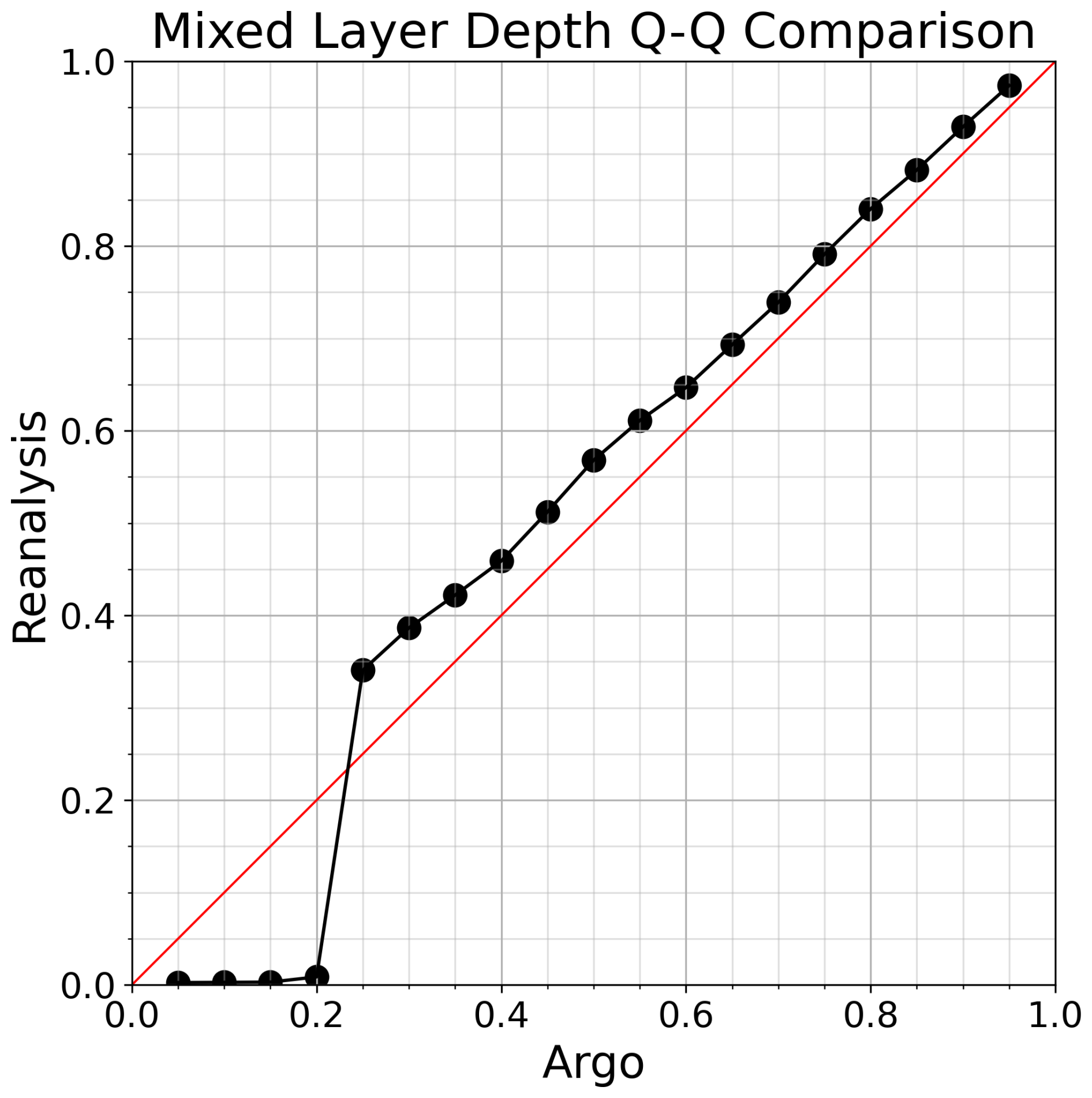
Figure 2 Quantile-Quantile plot comparing the reanalysis and Argo mixed layer depths. The red line is the 1 : 1 line.

As the methodology to determine d is based on EVT, the over representation of deep convection in the reanalysis can misrepresent the local dimensionality, as more system states will appear in the vicinity of true deep convection states than in observations. To make the MLD more representable of the actual system, misrepresentative states need to be removed. To keep the proper MLD states, we need information on deep convection before 2005, as this is the earliest data available from Argo profiles in the region. We also need more information for the year of 2015, as there is a gap in the Argo data there as well. The compilation of modelling and observation results from 1982 to 2013 in Somot et al. (2016) covers the first requirement and compiled observations in Margirier et al. (2020) cover the second requirement.

The deep convection years are taken to be the years with a maximum MLD below 1000 m in the region during the winter and spring. The threshold 1000 m is used as this is typically considered well within the Western Mediterranean Deep Water (WMDW; refer to Fig. 1 in Houpert et al., 2016). Once convection breaches the interface between the Eastern Intermediate Water (EIW) and WMDW at roughly 600, 1000 m is readily attained. In Fig. 3, these years are marked with filled dots: red for the reanalysis, black for the Argo data, blue for the information from Somot et al. (2016), and green for the information from Margirier et al. (2020). Empty dots denote non-convecting years. To the determine which reanalysis years are kept as deep convection years, they were compared to Somot et al. (2016), Margirier et al. (2020), and the Argo dataset. The two publications agree on overlapping years, however the Argo dataset disagrees with some years. For these disagreeing years, the determination was based on the publications' results (e.g. 2009). Years kept as deep convection years for the reanalysis are: 1987, 1991, 1992, 1999, 2000, 2003, 2005, 2006, 2009, 2010, 2011, 2012, 2013, 2018, and 2022. These years are marked by filled triangles in Fig. 3. The years when neither Somot et al. (2016), Margirier et al. (2020), nor the Argo dataset indicated a deep convection event were marked with a red empty “x”. These years are to be modified: 1988, 1989, 1993, 1994, 1995, 1996, 1997, 1998, 2001, 2002, 2004, 2007, 2008, 2014, 2015, 2016, 2017, 2019, and 2021.

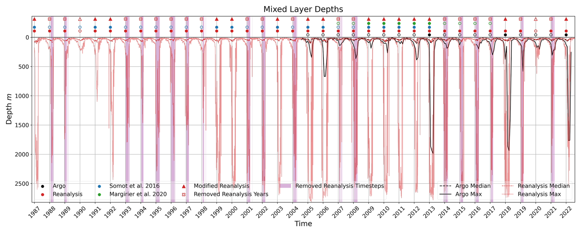
Figure 3 Mixed layer depth time series for the reanalysis and Argo observations with the occurrence of deep convection (as determined by a maximum MLD below 1000 m) from the reanalysis (red markers and lines), Argo observations (black markers and lines), Somot et al. (2016) (blue markers), and Margirier et al. (2020) (green markers). Filled dots mark deep convection years, unfilled dots mark non-deep convection years, and the filled triangles mark the years kept for the modified reanalysis MLD dataset. Empty red “x”'s denote removed years, with the purple shading more explicitly showing the time steps removed. The MLD maxima and medians were calculated daily for the reanalysis dataset over the spatial domain (consistent with the dataset's gridding). As the Argo MLDs were originally derived from profiles, the monthly maximum and median were taken for all values within the study area to compensate for the lower spatial coverage (Fig. 1).

The years to be modified in the reanalysis, according to Fig. 3, had the states (ergo time steps) removed when:

• the daily reanalysis maximum MLD reached below 250 m

• and occurred between 1 October of the previous year and 1 June of the current year

E.g. for the year 2004, the daily time steps when the reanalysis MLD maximum was deeper than 250 m and between 1 October 2003 and 1 June 2004, were removed. Here, 250 m is chosen as the threshold for removal, as this is a reasonable limit for when only intermediate mixing occurs (i.e. when the mixed layer doesn't breach the EIW/WMDW interface). This is corroborated by the typical maximum Argo MLDs observed during non-deep convection years in Fig. 3. In total, 1379 out of the 12 996 total, or 10.6 %, time steps were removed.

Comparatively, the original reanalysis MLD dataset had 94.4 % of the years as deep convecting (see Table 1). The revised set has 41.7 % of the years as deep convecting, which is more inline with both Somot et al. (2016) and Margirier et al. (2020) (51.6 % and 45.4 %, respectively; again refer to Table 1). The Argo MLDs alone appear to under represent deep convection at 17.6 %, but this is likely due to Somot et al. (2016) and Margirier et al. (2020) using more a complete set of observations (e.g. the Gulf of Lion mooring).

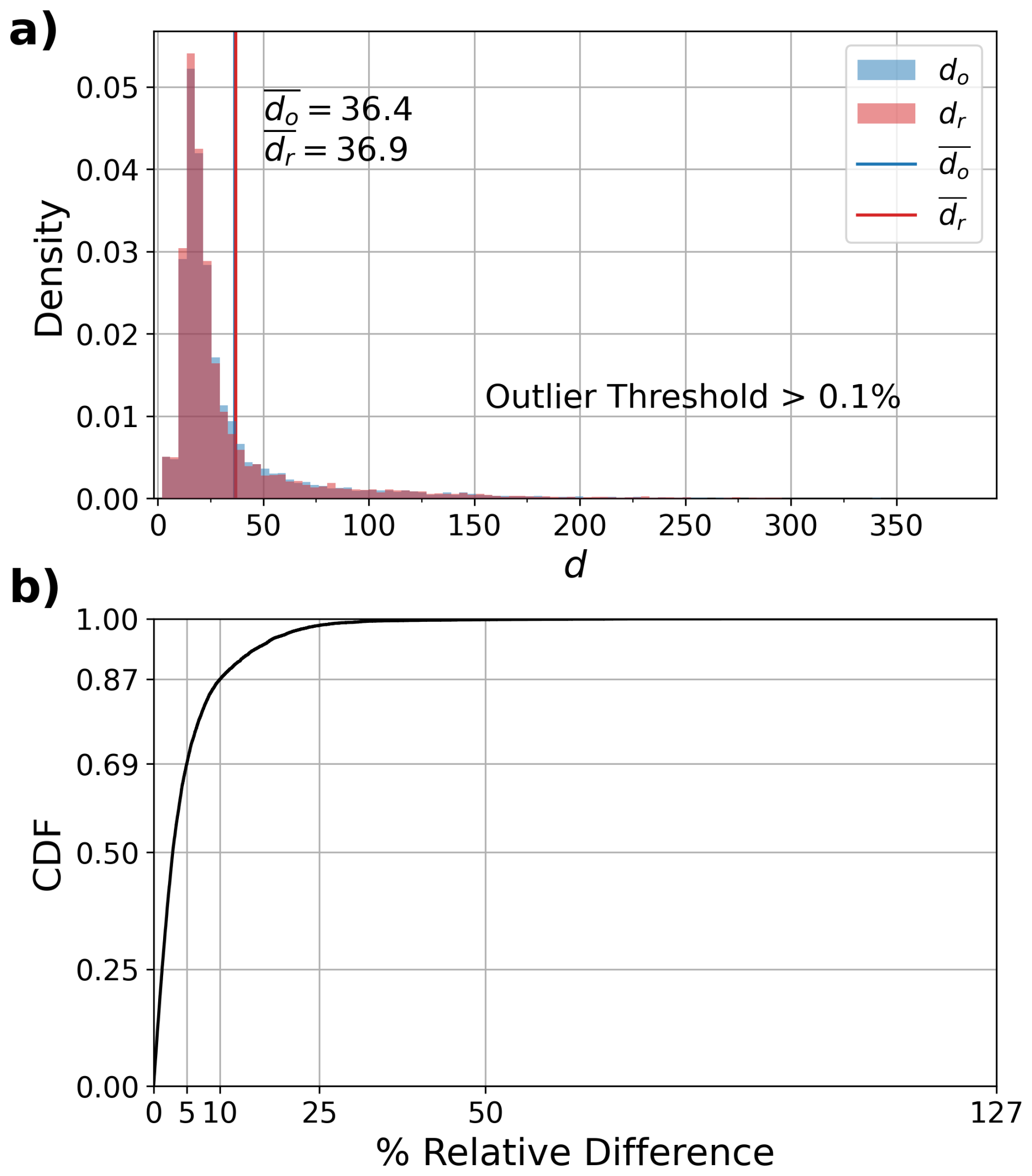
Figure 4 Differences in the distribution of local dimensionality between the original and revised dataset from the reanalysis (Escudier et al., 2021). d_o stands for the d calculated from the original reanalysis MLD set and d_r from the revised set. Panel (a) shows the density distributions of d_o and d_r. Outliers, determined as bins with counts less than 0.1 % of the population of either d are not displayed. The overbarred variables are the average values. Panel (b) shows the cumulative density function of the % relative differences (Eq. 2) between d_o and d_r (same time steps are compared). Note that the CDF(25) equals 0.986.

Escudier et al. (2021)Somot et al. (2016)Margirier et al. (2020)Holte et al. (2017)Escudier et al. (2021)

Table 1 Fractions (percentages) of deep convection (DC) and non deep convection (NDC) years in varying literature used to revise the mixed layer depth dataset from the reanalysis (Escudier et al., 2021).

^a Original CMCC reanalysis mixed layer depth dataset. ^b Argo mixed layer depth dataset. ^c Revised reanalysis mixed layer depth dataset used for the dynamical analysis.

Figure 4 shows the resulting difference between the distributions of d for the original reanalysis MLD dataset, d_o, and the revised set, d_r, in panels (a) and (b). Panel (a) shows the density distribution of d for both sets, while panel (b) shows the cumulative density function of the % relative difference, as describe by:

$$\begin{array}{}\text{(2)}& \mathrm{Relative}\mathrm{Difference}\left(t\right)={\displaystyle \frac{\left|d_{\mathrm{r}}\right(t)-d_{\mathrm{o}}(t\left)\right|}{d_{\mathrm{o}}\left(t\right)}}\cdot \mathrm{100}\end{array}$$

From Fig. 4b, we can see that 87.1 % of d_r differ by 10 % or less from their original values and 98.6 % of them are under 25 % different. Combined, with nearly identical distributions as seen in panel (a), the revised MLD set is more representative of reality while not significantly changing the results of the analysis. This is appears to be due to the relatively small number of time steps removed (10.6 %) for a statistically based method. The bulk of the time steps of the MLD still remain, keeping d_r close to their original values. N.B.: for the remaining sections of this work, unless otherwise mentioned, d will refer to d_r.

2.5 Sensitivity Analysis

Ideally, a large percentile of g₁ to determine T is used to drive the applicability of the EVT to problem at hand. However, doing so reduces the number of leftover exceedances (z) to form the GPD upon which the calculation of the local dimensionality relies (specifically the exponential distribution for this case). For this work, a potential question is whether the 98th percentile threshold for T is appropriate for the modified reanalysis dataset or not. Does the resulting distribution of z follow an exponential distribution? To answer these questions, the T and z were determined for multiple thresholds: 90th, 94th, 98th, and 99th percentile. The results are shown in Fig. 5.

Figure 5a displays the different distributions of T depending on the threshold chosen. The choice of threshold largely does not impact the resulting distribution except for the right-hand side. There is a peak for each threshold distribution that moves further positive along T and drops in probability with an increasing threshold. However, the difference between the 98th and 99th percentile is minimal. Panel (b) from the same figure displays the resulting distribution of z distributions. As a single z distribution is produced for each state, ξ (time step), the 25th, 50th (median), and 75th percentiles for the binned combination of these states/time steps were computed, per overarching percentile threshold. Each of these median distributions follow the exponential distribution qualitatively quite well, with each resembling the sample exponential distribution (d=25 for its scaling). This suggests that the choice of the 98th percentile for an effectively arbitrary threshold is appropriate for this study.

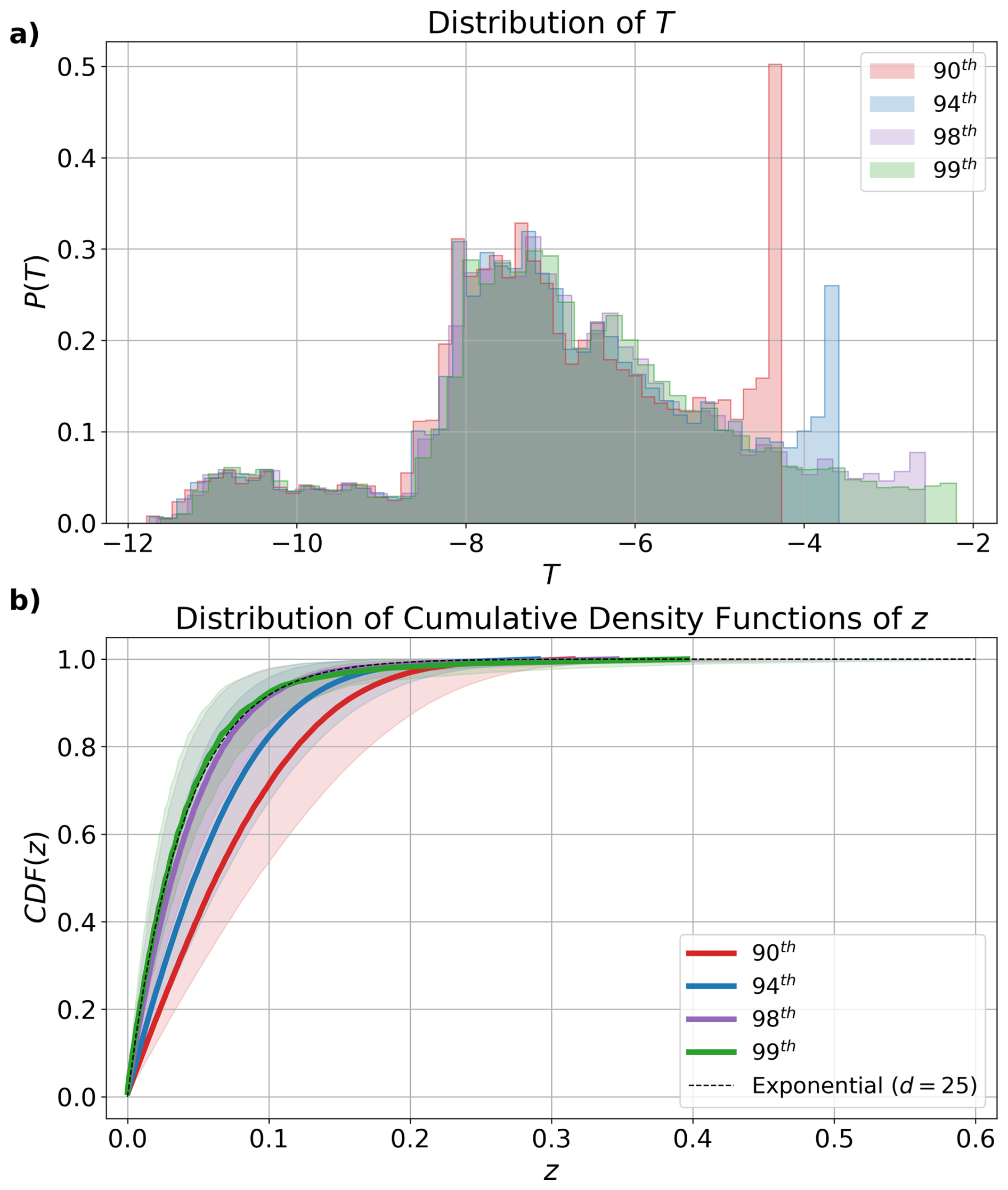
Figure 5 Results of the sensitivity analysis for different threshold limits: 90th, 94th, 98th, and 99th percentiles. Panel (a) shows the distribution of T from Sec. 2.1 for the respective percentile thresholds. Panel (b) shows the distribution of the cumulative density functions (CDF) of z, with the median displayed for each threshold and the region shaded between the 0.25 and 0.75 quantiles. An example exponential cumulative density function is also presented in (b) with a value of d=25 to define its shape.

3 Results

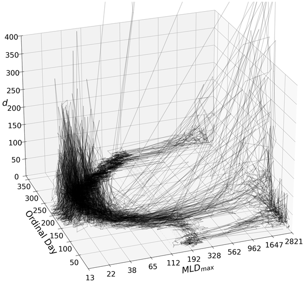
The resulting system trajectories of the local dimensionality of the MLD's fractal attractor are shown in Fig. 6. In essence, d describes the local, non-integer geometric dimension of the attractor (i.e. around 1 for a line, around 2 for locally planar, etc.). But, it also implies the predictability for a given state, albeit from a more relative standpoint. For the deep convection cycle, as measured by the mixed layer depth, d varies significantly throughout the years at different depths, yet with a clear annual cycle. The months with the larger local dimensionality are found either during the late spring and summer months (ordinal days ∼ 150 to ∼ 250) or during deep convection (ordinal days ∼ 0 to ∼ 100). Conversely, during the months of September through January (ordinal days from ∼ 250 to ∼ 365/366/0), the local dimensionality is quite low. Recalling that a larger dimensionality implies less predictability, these results suggest that the preconditioning period, when the MLD is deepening, is the most predictable period, requiring the least number of dimensions to describe. However, the summer months are the least predictable, despite the water column being the most stable (Margirier et al., 2020; Keller et al., 2024).

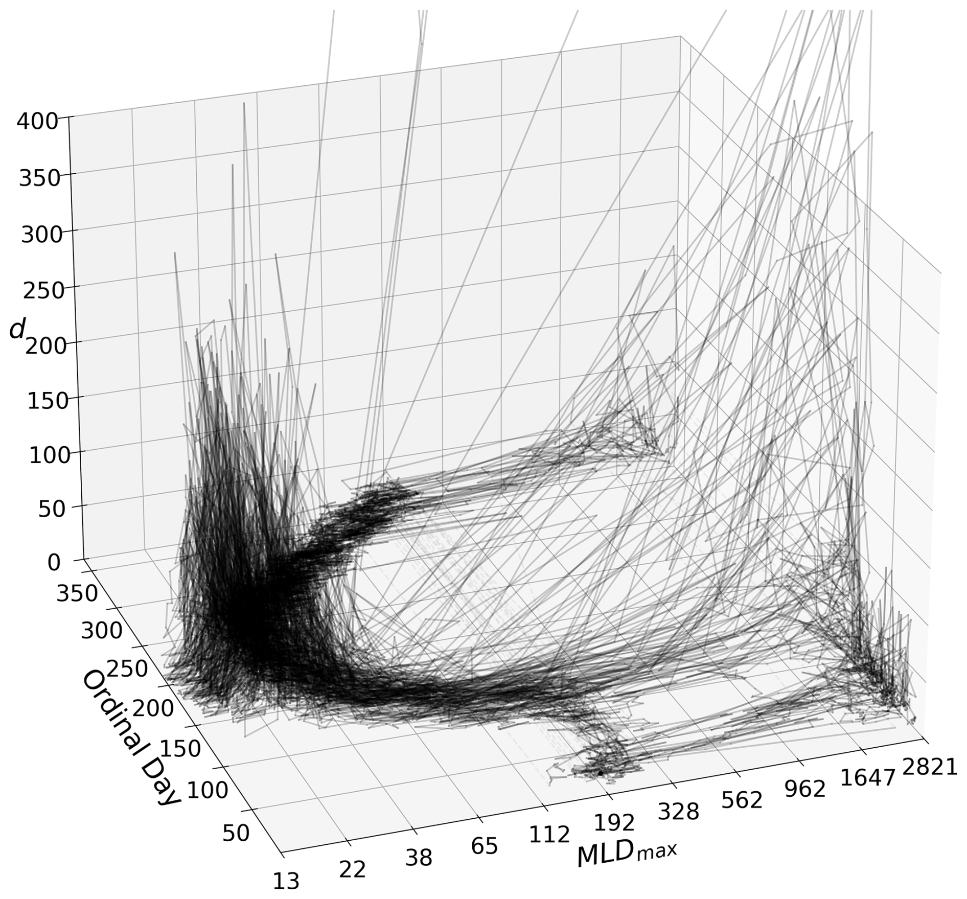
Figure 6 d trajectories of the modified MLD, marked by the maximum MLD on one axis (on a natural log axis), the day of the year on another axis, and the local dimensionality on the vertical. 28 values exceed 400 in the vertical (less than 0.2 % of all d) and are potentially random-process like. This is also visualized later in Fig. 9c). When the trajectories wrap around to the beginning of the year, the lines are lighter and dashed (the same is true for other large gaps in the trajectories from modifying the MLD dataset).

Initially, it appears that the local dimensionality is quite large during deep convection from Fig. 6. However, if we look at individual trajectories, such as those shown in Fig. 7, this isn't always true. Panel (c) shows for the exceptional case of the winter of 2012/2013, values sometimes exceed 400, agreeing with its exceptionalness. However, for winter of 1991/1992, shown in panel (b), d during the deep convecting period remains quite low and less than that in the restratification period and summer. A non deep convecting winter, shown in panel (a) (2015/2016), behaves similarly.

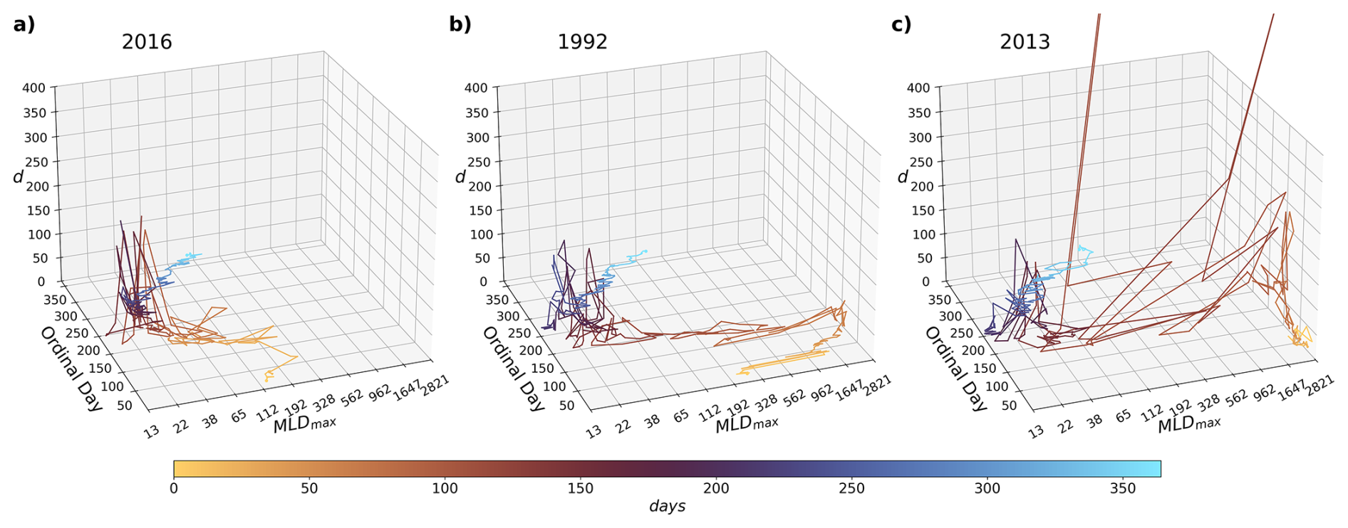
Figure 7 Selected yearlong trajectories from Fig. 6, from the initial day of the year til the end. The trajectory in (a) shows the path for the year of 2016 (winter 2015/2016; a non deep convecting year) and the trajectory in (b) shows the path for the year of 1992 (winter 1991/1992; a deep convecting year). Panel (c) shows the year of 2013 (winter of 2012/2013). The axes are the same as for Fig. 6, with the added visual aid of a color map for the time progression of the trajectories.

To get a clearer image of the seasonal distribution of d and see its behavior during the different deep convection cycle periods, Fig. 8 shows the monthly median, 25th, and 75th quantiles of both the d (panel a) and MLD maximum (panel b). From this figure, we can confirm that the summer months, particularly from May to September, show an enhanced local dimensionality. Additionally, we can confirm that the preconditioning period, from September to January is also the lowest, with the lowest spread in values. This is followed by the deep convecting and restratification periods, which have slightly higher values of d (comparing panels a and b from March to May). This demonstrates that typically the local dimensionality during the deep convecting period is lower than the summer months, despite having some exceptional cases.

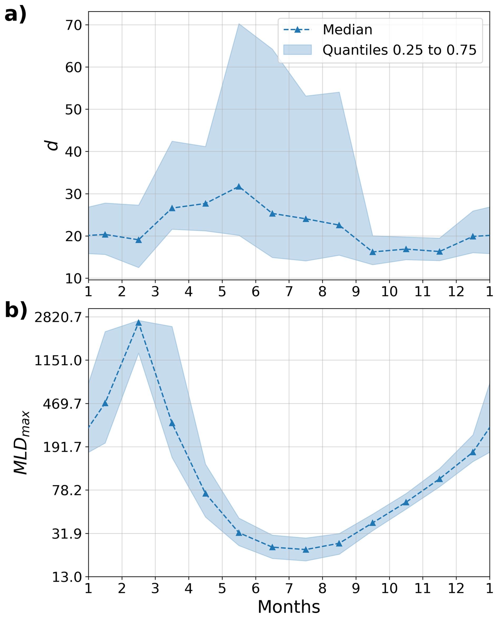
Figure 8 Seasonal distributions of d (a), and MLD maximum (b). The monthly medians are shown with the triangular markers and dashed lines, while the shading shows the region between the 25th and 75th percentiles. Note that the vertical axis for (b) is natural logarithmic, again due to the logarithmic spacing of the vertical cells in the reanalysis model.

If we take Fig. 8 a step further, and look at the distribution of d with depth and time, then the local dimensionality of the deep convection cycle becomes more nuanced. When we now look at the median d during deep convection, focusing on Fig. 9b and c, we see that only part of the deep convection period is less predictable: the events with MLD maximum depths occurring partially in March, and during April and May, where d has quite a few values exceeding 100. Deep convection with MLD maxima during December, January, and February have much lower values for d, around 15 to 50. These states are more comparable to the states with less deep MLD maxima found during the middle of the restratification period or when vertical mixing stays within the Eastern Intermediate Water layer. Notably, the regions of MLD maxima with large d, have values approaching 8000 (hence why they were separated into panel c), with relatively large values surrounding this patch as well. This suggests that this region is more characterized as a random process, as random behavior tends to have values at or approaching infinity for d, as it takes an infinite number of dimensions to accurately describe (Victor, 1987; Argyris et al., 1998; Kondrashov et al., 2019) (but finite values of d for certain categories of random attractors exist; Debussche, 1997, 1998). Figure 9a and d also show this region contains a low number of system states (seen in panel a as the percentage of time steps present per bin) and mixed variability (seen as the difference between the 75th and 25th percentile of d per bin), lending support to the idea that these states are better characterized as a random process. Additionally, this could be viewed as random behavior at the onset of restratification near the end of the deep convection period.

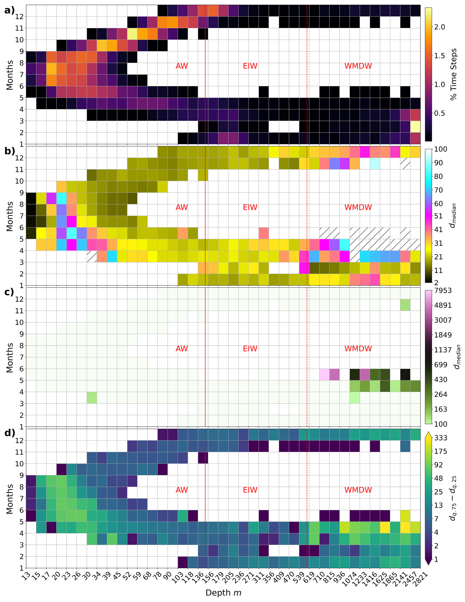
Figure 9 The seasonal and depth distribution of d, binned with respect to time and maximum MLD depth. Each bin is one month wide and has a depth side varying exponentially (increasing with depth). Panel (a) shows the percent occurrence of states within each bin. Panels (b) and (c) both display the medians of d, with the (b) showing 2 to 100 and (c) showing from 100 to the maximum value. Hatching in (b) indicates bins that exceed 100. Panel (c)'s color bar is in log base 10, to more easily see the value separation versus natural log used for depth. Panel (d) shows the variability of d via the difference between each bin's 0.75 and 0.25 quantile. The Atlantic Water (AW), Eastern Intermediate Water (EIW), and Western Mediterranean Deep Water (WMDW) are shown with their general layer bounds: 0 to 150, 150 to 600, and 600 m and below, for each layer, respectively.

Returning back to the other system states, Fig. 9b confirms that during the months of September to the beginning of January, the local dimensionality is very low. Panel (d) reinforces this by showing that this region of phase space is also relatively low in variability despite having many time steps present (panel a). Panel (b) also confirms that d is larger during the summer months, with values around 35 to 90 (sometimes around 100), albeit, when the system is restabilizing the MLD. Instead, we can see the deeper MLDs leading into the preconditioning period, during the months of June, July, and August, have quite a low dimensionality, with values around the single digits to 20. We can also see the shallowest MLDs during these months have the lowest d over the whole distribution, approaching values of 2. With a dimensionality of 2, the fractal attractor's shape is locally a plane. This isn't clearly visible in Figs. 6 or 8, therefore, Fig. 9b) clarifies that the summer months are the least predictable during the restratification period but are otherwise the most predictable system states.

4 Discussion

In geophysical fluids, the nonlinear, advective term in their mathematical description is the source of chaos in their systems (Lorenz, 1963). We can reason that the restratification period is the most consistently unpredictable part of the deep convection system, because the tracer field is dominated by horizontal gradients, as the less dense water surrounding the deep convection patch tries to reestablish a spatially stable density gradient. The baroclinic instability breaks apart the rim current (Madec et al., 1991), forming eddies that capture and maintain portions of the mixed patch to be transported elsewhere in the western Mediterranean basin (Bosse et al., 2016; Testor and Gascard, 2003). Conversely, the growth of the ocean MLD occurs non penetratively, even during deep convection, with the slow erosion of the density gradient without entraining plumes (Marshall and Schott, 1999). Therefore, the fluid itself and its tracers (salinity and temperature) at the interface with denser waters are relatively less turbulent. The findings here support the hypothesis of Waldman et al. (2018) that baroclinic instability generates much of the intrinsic variability in the deep convection system. In their work, they attributed the spatial intrinsic variability to the spatial variability of the baroclinic instability, as measured through a bathymetry aware Eady eddy theory (Blumsack and Gierasch, 1972; Isachsen, 2011, 2015). For this work, the method captures the spatial variability but only provides us a with the instantaneous variability of the system in time, therefore the results here can only concur with Waldman et al. (2018)'s findings qualitatively.

A key point to note about using this methodology is that it measures the local dimensionality of a particular system. Therefore, while here it describes the chaotic behavior of the underlying fractal attractor of deep convection, it fundamentally relies on the particular model used to represent this phenomenon, which in this case is NEMO. NEMO has been used extensively to investigate deep convection in the Gulf of Lion (Waldman et al., 2018, 2017a; Lebeaupin Brossier et al., 2017; Houpert et al., 2016; Waldman et al., 2017b; L'Hévéder et al., 2012; Lebeaupin Brossier et al., 2012; Beuvier et al., 2012; Herrmann et al., 2010; Lebeaupin Brossier and Drobinski, 2009), and so the analysis here is relevant. However, NEMO employs a number of assumptions that could affect the transferability of this analysis. It employs the spherical Earth and thin shell approximation, neglects the cosine component of the Coriolis rotation vector, and assumes the turbulent closure, Boussinesq, hydrostatic, and incompressible fluid hypotheses. The last four assumptions could potentially alter the analysis presented here if they are relaxed or removed, as all four involve some level of nonlinearity. Additionally, the hydrostatic hypothesis has the consequence that the convective process in NEMO (and other hydrostatic models) is parameterized, and, depending on its implementation may or may not introduce more or less nonlinearity (as convection is inherently a nonlinear process). Therefore, using this analysis with an idealized, nonhydrostatic version of deep convection would be needed to determine if it is sensitive to convection being parameterized or not.

5 Conclusions

The results shown here present a general progression of the predictability of the deep convection system in the Gulf of Lion. Starting from the late the summer months, the system is relatively quite predictable, with a local dimension ranging from 10 to 20. As the system enters the preconditioning period and the MLD deepens, the local dimension slowly grows, sometimes reaching 30 by the turn of the year. If deep convection occurs, the system sees an increase in its local dimension to around 15 to 50, if the system restratifies before March. Otherwise, the system appears to behave randomly with exceedingly large values. Once the system restratifies and the MLD decreases, the largest, non-random states are found during the end of the restratification period, with the local dimension ranging from 35 to 90. Counter-intuitively, these large values are found squarely during the summer months. With that said, the system can also reach an effectively locally planar state during the summer, if it becomes exceedingly stable.

From this analysis, the restratification period is consistently more chaotic and less predictable than the deep convection period, with some exceptions. As the restratification period sets up the conditions for the (potential) proceeding deep convection process, after a very predictable preconditioning period, better recreating and better understanding the restratification process may improve the reproducibility of deep convection in modelling efforts. This could be particularly important for long running simulations, with multiple restratification periods, and therefore, warrants further investigation.