Conditional updates of neural network weights for increased out of training performance

This study proposes a method to enhance neural network performance when training data and application data are not very similar, e.g., out of distribution problems, as well as pattern and regime shifts. In contrast to previous approaches to out of distribution problems, which alter the inputs and outputs of an operator, our approach alters the operator itself. Here, we especially aim to alter the weights and biases of a neural network to mitigate the out of distribution problem. The method consists of three main steps: (1) Fine-tune a trained neural network towards reasonable subsets of the training data set and note down the resulting weight anomalies. (2) Choose reasonable predictors and derive a regression between the predictors and the noted weight anomalies. (3) Extrapolate the weights, and thereby the neural network, to the application data. We show and discuss this method in three nonlinear use cases from the climate sciences, which include successful temporal, spatial, and cross-regime extrapolations of neural networks.

1 Introduction

In physics, especially in nonlinear geosciences and climate sciences, the poor performance of neural networks (NN) when applied outside their training distribution or their trained dynamics poses a very strong limitation to their general applicability (Irrgang et al., 2021; Landsberg and Barnes, 2026).

In these fields, physical relations such as laws, dependencies, or sensitivities are commonly derived (or learned) under well-observed conditions and are then applied to less-observed conditions to gain knowledge about the latter. For example, results from lab or numerical model experiments are regularly applied to real-world problems or observations (e.g., Mehta et al., 2025); knowledge from our Earth and our Solar System is transferred to other planets and other star systems (e.g., Kvorka et al., 2026); learned relations that are derived today are transferred to the distant past, or to the future (e.g., Eyring et al., 2016; Wang et al., 2024; Koutsodendris et al., 2014). Usually, well-documented problems are transferred, e.g., across country borders (Sebastianelli et al., 2024; Kotz et al., 2021), across spatial scales (Ortega-Cisneros et al., 2025), from the well-observed upper ocean to the deep ocean (Llovel et al., 2014; Lee and Gentemann, 2018), or from the lower latitudes to the poles (Irrgang et al., 2020); or a mixture of it all (Jung et al., 2024; van der Deure et al., 2025).

From a machine-learning perspective, this means that available training data are typically limited in their spatial and temporal extent, as observations or model simulations only cover specific time periods or regions. For example, Earth observing satellites often leave the higher latitudes unobserved depending on their inclination (e.g., Li et al., 2025); oceanographic Argo floats measure only the upper 2000 m of the marine water column (e.g., Wong et al., 2020); paleo records such as ice cores may exist for the past but only in regions where there is still ice today (e.g., Bereiter et al., 2015). In general, since the onset of satellite measurements, the majority of Earth observations cover only the last few decades; no measurements exist for the future, and comparatively few measurements exist for the distant past. Furthermore, the environmental conditions that exist on Earth are very heterogeneous (e.g., Peel et al., 2007), and most processes, for instance, the climate, are non-static in nature (e.g., Schannwell et al., 2024). The combination of spatiotemporally-localized data distributions in combination with differing conditions between possible inference regions/times/environments and the application regions/times/environments makes it very difficult for NN to operate (e.g., Rasp et al., 2018; Hernanz et al., 2022; Hsieh, 2023).

In some cases, individual standardization or rescaling of the variables from the application data set is a valid option to mitigate the out of distribution (OOD) problem. However, in many real use cases, the standardization or rescaling removes essential information from the application data. This is true for nonlinear problems where standardizing or rescaling the input will lead to wrong outputs, as by the definition of non-linearity: $f(a+b)\ne f\left(a\right)+f\left(b\right)$ and $f(n\cdot a)\ne n\cdot f\left(a\right)$. Especially in the climate sciences, the conditions for contemporary artificial intelligence (AI) are challenging and raise the demand for new approaches (e.g., Eyring et al., 2024; Beucler et al., 2024; Fang et al., 2025; El Ghawi et al., 2025; Qin et al., 2025). For example, removing offsets and trends in variables such as sea level and temperature would discard information essential for predicting climate change, climate impacts, and tipping. Likewise, the amplitudes of extreme events should not be rescaled to fit those of the training data. In addition, standardization and rescaling require a certain amount of data points, which are not always available in the application data. Often, the learned relations have to be applied to one single (possibly extreme) event, to a few ice cores, to one other planet, moon, or star system, and so on, i.e., they pose so-called single-shot or few-shot problems in AI terminology. Consequently, in such cases, application-distribution-based standardization, rescaling, remapping, or basis transformation (e.g., Beucler et al., 2024) is not possible. Finally, even without any distribution shift or with normalization, the NN can still be confronted with unseen combinations of input values, which can pose a serious OOD problem.

Here, we propose a method to reduce this problem for NN by exploiting the NN's own sensitivity towards samples of the training data to predict NN weights and biases, which are intended to perform better in the OOD application realm (cf. Sect. 2, Method).

However, this paper does not discuss if and when NN are suitable choices for nonlinear OOD problems. Furthermore, we will not discuss (in depth) the many other methods that might be able to extrapolate the inputs or outputs of some NN to OOD regions. The reason is that many tasks do require NN, especially when these other approaches cannot be used. Examples of these tasks include reasoning and decision making, conditional generative AI, big data, and large classification problems such as image feature detection. These are applications in which extrapolating or averaging (cf. Hsieh, 2023) NN output will not give meaningful results. Our study focuses on problems where NN are used for various reasons (ease of use and implementation, existing workflows, compute limitations, invertibility, lack of alternatives, etc.), and these NN may be used on OOD data. Still, for completeness, we provide a comparison of our experiment 1 results to several standard extrapolation methods in Appendix A, together with a brief discussion.

We think that AI applications in many fields of physics and other fields of science, such as medicine, biology, economic sciences, or social sciences, can benefit from the proposed method. Nonetheless, we demonstrate and evaluate the proposed methodology in three classes of experiments that are mainly motivated by climate sciences and Earth sciences (cf. Sect. 3, Experiment Design and Data). One experiment where NN weights are predicted through time, one experiment where NN weights are predicted through space, and one experiment where NN weights are predicted across regime boundaries. Within similar training and application data sets and domains, the chosen experiments do not represent any challenges to NN training (nor to basic mathematics and physics). The challenges we demonstrate and mitigate here arise only by training the NN in times and places that have very different conditions than the times and places the model has to operate on during application. Consequently, these experiments should be understood entirely as symbols or placeholders for more sophisticated AI tools.

2 Method

The proposed weight-prediction method for NN follows the pseudo-code given in Box 1. At its core, the approach applies existing extrapolation techniques to the weights of a NN instead of applying them to the input and output of NN as other approaches suggest (e.g., Hsieh, 2023; Beucler et al., 2024).

Our approach consists of 3 parts. After training of a suitable NN for the problem at hand with a training data set (Box 1, step 1), one has to do the following. (A) For each weight and bias of this hereafter termed “parent model”, collect the weight deviations arising from retraining the parent model with single data points or subsets of the training data set (Box 1, step 2). (B) For each weight and bias of the parent model, establish a dependency between said weight deviations and suitable predictors, e.g., a linear regression (Box 1, step 3). (C) For each weight and bias of the parent model, extrapolate the established dependency towards application data points and thus generate new application-data-tailored NN, the “child models” (Box 1, step 4). From now on, we summarize a group of child models originating from the same trained parent model (cf. ParentModel₀ in Box 1, step 1) under the singular “child model”. All models in one child model differ only due to the fact that their weights are predicted onto different application data points (cf. x_a and ChildModel_a in Box 1, step 4), until this step, they are based on exactly the same data. Consequently, if we use the plural from now on, we refer to different child model groups, i.e., groups originating from different ParentModel₀.

Box 1 Pseudo-code of the weight-prediction approach.

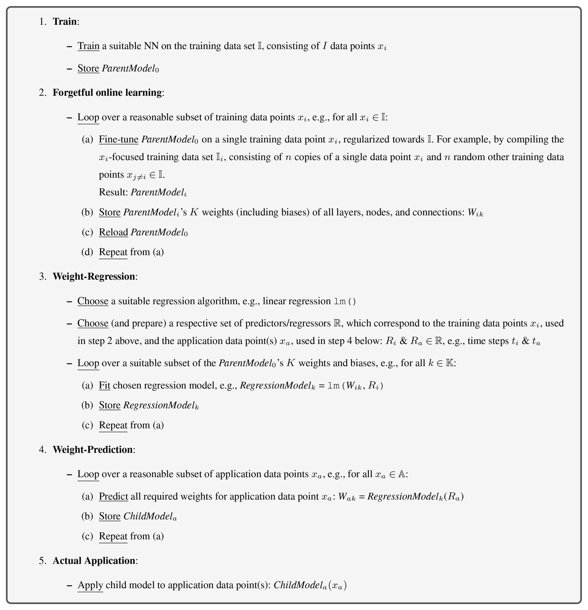
The reasoning why the above approach should work is that fine-tuning the ParentModel₀ further on a training data point x_i can result in a new model (ParentModel_i) whose weights and biases differ (a) only slightly and (b) in a meaningful way from ParentModel₀. Ideally, all ParentModel_i form a point cloud around ParentModel₀ in NN parameter space, which encodes the respective sensitivities between this specific ParentModel₀'s weights and the input data. For this to be the case, the deviations between ParentModel₀ and the related ParentModel_i have to be constrained in a way that no entirely new and therefore unrelated ParentModel_i are created in the process. In other words, all ParentModel_i should be closely yet meaningfully distributed around ParentModel₀. To achieve this, it should be theoretically sufficient to restrict the fine-tuning of ParentModel₀ (cf. Box 1, step 2a) towards each x_i to a few update steps (epochs). However, we found that a regularized fine-tuning of ParentModel₀ towards individual training data points x_i works better and allows for more flexible fine-tuning approaches. To regularize the fine-tuning step, we add a representative fraction of the training data to the x_i fine-tuning batch. Naturally, the impact of such a regularization and the impact of the fine-tuning towards a single x_i in generating a new ParentModel_i has to be weighted reasonably. Box 1, step 2a gives an example of how to achieve a suitable regularization easily in practice, e.g., we take n random samples from the training data combined with n duplicates of x_i to ensure equal weighting in the fine-tuning batch. Consequently, weighting in the given example is 0.5 for each impact, i.e., equal impact from the entire training set (𝕀) and from a single data point x_i.

To choose a suitable approach for the ParentModel_i generation (Box 1, step 2a), the distribution of the ParentModel_i around ParentModel₀ can be easily plotted and analyzed, since this distribution does not depend on OOD data. The analysis could either focus on single weights or be based on a NN-wide integral view of weight differences between the ParentModel_i and ParentModel₀.

Note, in Box 1, we show a total-valued form of the method. Naturally, handling only the weight anomalies or increments ΔW_ik is equally possible.

The exact execution of each given step of the core approach (Box 1) can vary substantially and should be adapted to the problem at hand and to domain knowledge if available. For example, two main choices have to be made during the approach. First, choices for suitable predictors for the weight-regression (Box 1, step 3) and the subsequent weight-prediction (step 4) have to be made. It is out of the scope of this paper to discuss these choices here in detail. Ideally, the choice should be heavily influenced by prior knowledge of the problem at hand. Especially, how the problem might behave outside the training data range. In principle, the predictors for the weights can be anything, e.g., (i) time, (ii) (subsets of) the original NN input, (iii) features derived from the original input, or (iv) additional information not used by the parent NN model. A careful selection and pruning of the predictors is advised. In our examples, we demonstrate the use of (ii) in experiment 2, and (iii) in experiments 1 and 3. Note that in experiment 2, the inputs of depth, latitude, and longitude are not necessary for the NN to calculate the correct sea water density as long as temperature, salinity, and pressure are given. However, they are promising weight-predictors. As we did not want to limit the parent NN by withholding information, we unified the inputs of parent NN training and weight-regression in experiment 2, i.e., the weight-predictors are deliberately included in the NN inputs.

Second, a choice for the weight-prediction method has to be made. Of these, many suitable exist, e.g., auto-regressive integrated moving average (ARIMA), eXtreme Gradient Boosting (XGBoost), Gaussian Processes, linear models (LM), generalized linear models (GLM, Nelder and Wedderburn, 1972), generalized additive model (GAM, Hastie and Tibshirani, 1986), support vector machines (SVM, Cortes and Vapnik, 1995), random forest (Ho, 1995), NN itself (cf. Chauhan et al., 2024), and many more. Again, it is not part of this paper to review regression methods and their rightful application. Nonetheless, we provide a comparison of these methods acting on our toy problems in Appendix A. In experiments 1 and 2, we chose LM for their ease of use and very fast computation. The latter is especially needed as we do regression and prediction for every weight and bias of every single node of the NN. However, if the NN is very large, low-rank adaptation (LoRA, Hu et al., 2021) or similar decompositions should be considered. We would not generally recommend using other purely data-driven methods like RF and NN as they suffer from poor OOD performance, as already stated (e.g., Rasp et al., 2018; Hernanz et al., 2022; Hsieh, 2023). Still, in some cases, we found improvements in our experiments by these methods. For instance, in experiment 3, we demonstrate the use of a NN for the weight-regression and weight-prediction tasks. In general, if you know a regression method that works well for your problem, domain, or data (cf. Figs. A1–A3), then this method could be a good candidate for extrapolating the weights of a NN (if the method is fast enough, that is).

3 Experiment Design and Data

3.1 Experiment 1: Tipping of the Atlantic Meridional Overturning Circulation

We base experiment 1 on van Westen et al. (2024), a paper that shows that critical weakening of the Atlantic Meridional Overturning Circulation (AMOC) strength can occur in complex climate models. This so-called AMOC tipping is triggered by forcing the northern Atlantic Ocean of the respective climate model with increased freshwater flux (e.g., related to the rapid melting of the Greenland Ice Sheet). The paper's supplementary material and the data we use here is located in the following repository: https://github.com/RenevanWesten/SA-AMOC-Collapse/tree/SA-AMOC-Collapse_v1.0 (last access: 1 August 2025). These hosing experiments are a common tool in climate sciences (e.g., Rahmstorf, 1996; Saynisch et al., 2016).

As input to the NN, we use 2d velocity fields representing vertical slices through the Atlantic Ocean along the latitude of 26° N, i.e., the maps of meridional velocity (VVEL). These model-based maps of horizontal velocity are always taken at the same location and are given as annual values. The VVEL data can be downloaded from the above-given repository from the folder: /Data/CESM/Data/AMOC_section_26N/. The files cover each 50 years of data; the first one is called CESM_year_0001-0050.nc (and so forth).

The target output of the NN is the strength of the AMOC given in Sverdrup (1 Sv =10⁶ m³ s⁻¹), i.e., a single value per input velocity map. The AMOC strength is defined as the total meridional volume transport at 26° N over the upper 1000 m (cf. Eq. (3) in van Westen et al., 2024). The respective AMOC strength time series is given in /Data/CESM/Ocean/AMOC_transport_depth_0-1000m.nc

The challenge in experiment 1 is that the training is based only on data before the AMOC tipping point, occurring around year 1800 of the model data, cf. Fig. 1. However, the NN has to calculate the correct AMOC strength also during tipping and even after tipping, a serious OOD problem.

3.2 Experiment 2: Estimation of Sea Water Density

Experiment 2 is based on the highly nonlinear Equation Of State for sea water (EOS). For every desired oceanic location, the NN input is salinity (S), temperature (T), pressure (P), latitude (ϕ), longitude (λ), and depth (z). The target output is the local in-situ density (ρ) at this particular location. Consequently, the NN task is to convert 6 numbers into one. For data, we use the gridded observations of the World Ocean Atlas (Locarnini et al., 2024; Reagan et al., 2024), which are available under https://www.ncei.noaa.gov/access/world-ocean-atlas-2023/ (last access: 1 September 2025). We use the 5° decadal averaged annual fields of S and T for every available latitude (36 levels), longitude (72 levels), and depth (102 levels) of the provided 3d ocean grid. These values represent long-term averages, and no temporal dimension is present in this experiment. We then calculate P and ρ by using the routines swPressure(z,ϕ) and swRho(S,T,P) from the oce R-package (Kelley and Richards, 2025), which follow the Thermodynamic Equation Of Sea Water – 2010 (TEOS-10) standards (IOC et al., 2010).

Experiment 2 is motivated by the diminishing of oceanic monitoring capabilities with depth. Let's assume that we have found an interesting relation between our targets and the Argo float data. Unfortunately, the Argo floats cover only the upper 2000 m of the water column (Wong et al., 2020). However, we want to exploit our findings also below 2000 m. In a practical application case, this relation could estimate krill, CO₂, or nutrients. Here, we restrict ourselves to the estimation of sea water density.

In contrast to experiment 1 where knowledge has to be transferred over time (actually, also over to a different post-tipping dynamic), the challenge of experiment 2 is to transfer learned knowledge spatially. The training of the NN is restricted to a spatial (upper) subset of the world oceans. However, the trained NN has to redo the calculation for the entire ocean where OOD input and OOD output values occur. A further difficulty is that the EOS follows a complicated, highly nonlinear empirical polynomial (cf. Roquet et al., 2015).

3.3 Experiment 3: Uncertainty Estimation of Global Wind Velocity Reanalyses

The third experiment focuses on cross-regime extrapolation of learned uncertainties in global wind velocity reanalyses. The setup follows the concept proposed by Irrgang et al. (2020), who demonstrated that spatiotemporal uncertainty patterns learned at a single oceanic location can be generalized to the global ocean domain. Here, we extend this approach by transferring the learned uncertainty information from a single oceanic reference point to continental regions. Since wind dynamics over land are governed by different boundary-layer processes, surface roughness, and convective regimes compared to those over the ocean, this setup represents a severe OOD scenario.

In contrast to Irrgang et al. (2020), who used three atmospheric reanalysis products as model input, we restrict the input data to two widely used reanalyses: ERA5 (Hersbach et al., 2023) from the European Centre for Medium-Range Weather Forecasts (ECMWF) and CFSv2 (Saha et al., 2014) from the National Centers for Environmental Prediction (NCEP). Data set preparation, NN model architecture, and NN model training follow the same strategy as in the reference study to ensure comparability. This configuration tests whether the learned sensitivities in wind velocity uncertainty over marine environments can meaningfully generalize to terrestrial conditions.

4 Results and Discussion

4.1 Experiment 1: Tipping of the Atlantic Meridional Overturning Circulation

Notable deviations in experiment 1 from the recipe given in Box 1:

• Skipped step 2c (reload ParentModel₀)

• EOF of the ParentModel₀ inputs are used as weight predictors

To predict AMOC strength from velocity maps, we use a standard shallow convolutional NN (CNN), with 2 convolutional/max pooling layers followed by two dense layers. The last layer has linear activation, and all other layers have the Exponential Linear Unit (ELU) activation. For the fine-tuning regularization (Box 1, step 2a), n is set to 200.

For the regression of the NN weights, the predictors are based on the decomposition into empirical orthogonal functions (EOF) of the NN's training data inputs. The principal components of the 4 leading EOF, i.e., 4 numbers per time step (respectively per velocity field), are used for the regression of the NN weights. Outside the training data, exactly the same EOF-basis as during training is used to decompose the velocity maps. Another possible set of predictors could be mean, maximum, minimum, and standard deviation of each individual velocity map, i.e., again 4 numbers per time step, or even time itself if a suitable low-dimensional bifurcation model were to be employed for the NN weight-prediction (cf. Rahmstorf, 1996). Note, however, that the sensitivity of the weights is not dictated by the domain dynamics alone but also depends on the involved activation functions (and not only the activation function from the node under consideration). For example, if a complex nonlinear change of model output is required by the application domain dynamics, it can, in principle, be realized by a less complex (e.g., linear) weight change when nonlinear activation functions are involved. Furthermore, the required weight changes can be distributed over several layers, which then will entangle all contributing activation functions.

As there is a clear order of the data in experiment 1, i.e., the temporal order, we skip the “reload ParentModel₀” step of the approach (cf. Box 1, step 2c). This way, the online learning is not forgetful, and the weights will evolve continuously along the time axis as the AMOC system does itself. This improves the results in this experiment as it reduces noise in the generation of the weight sensitivities W_ik. After establishing weight-predictor relations for every weight and bias of the CNN, including the CNN layers, the child model is predicted with sub-models (cf. ChildModel_a) for every single time step of the problem by using the same weight-predictor relations. Each of these sub-models is then applied to one single data point, i.e., time step, only.

Figure 1 shows the time series of the target value (black line), the output of the parent model (red line), and the output of the same model after the application of the weight-prediction approach (orange line), i.e., the child model. The training data starts at year 1, and the end of the training data (EOT) is shown by a vertical dashed line, here at 800 years. After the tipping of the AMOC sets in at around 1800 years, the parent model has clearly problems reproducing the black line. Its output is strongly biased towards the output it had learned during training. The child model surpasses the parent model in its performance during and after tipping.

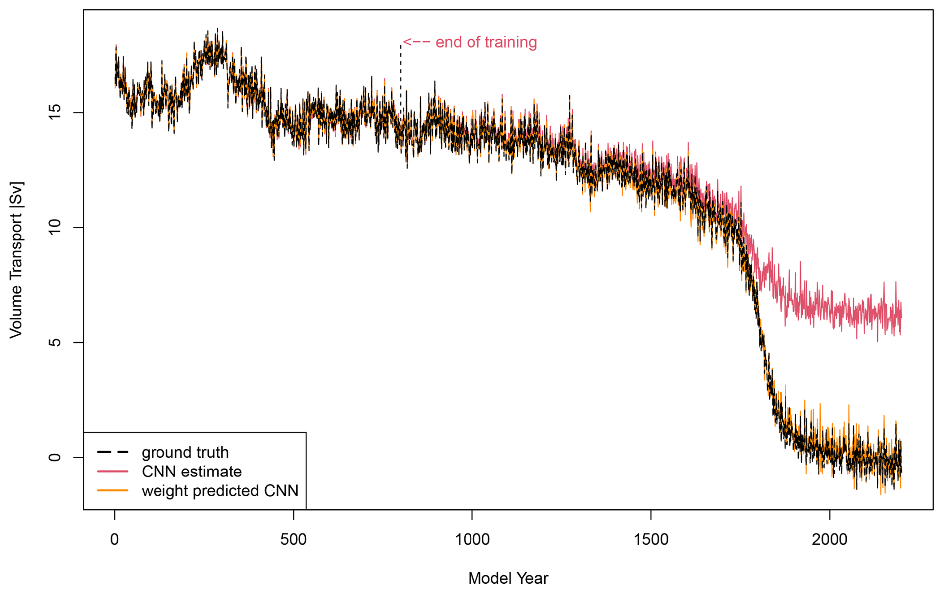
Figure 1 AMOC strength and an example of good performance of the weight-prediction method. Black Line: AMOC overturning decay and tipping, i.e., the target ground truth values. Red Line: Output of parent model trained until the dashed end of training (EOT) line. Orange Line: Output of weight-predicted child model. Online learning and subsequent fitting of EOF-to-weight relations used only data before the dashed EOT line.

Please note that since ParentModel₀ is not reset during step 2c of Box 1, at the end of step 2 we get a NN model that has seen the training data more often than ParentModel₀. Still, the performance of this model (not shown) is the same as that of ParentModel₀, and the improvements plotted in Fig. 1 must be attributed entirely to steps 3, 4, and 5 of our approach.

Since in general, the training of NN can have largely varying results, we repeated the experiment several hundred times with randomly varying EOT times, while the beginning of the training window remained fixed at year 1. As a consequence, the amount of data each NN is trained on varies, as well as how close the EOT comes to the actual tipping event. Furthermore, two weight-regression methods are tested. The results are aggregated in Fig. 2.

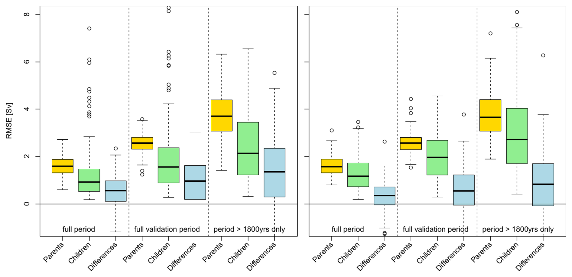
Figure 2 Impact of the choice of the weight-prediction method on the child model performance. Polynomials of order 1 (left panel) and order 2 (right panel) were fitted to the leading 4 principal components of the input variable (i.e., the meridional velocity maps). Yellow Boxes: RMSE of parent models. Green Boxes: RMSE of child models. Blue Boxes: Pairwise RMSE differences (i.e., unperturbed “parent” model minus corresponding weight-predicted “child” model). Positive values represent improvements due to the presented weight-prediction approach. Note that “full period” and “period > 1800” are the same for every simulation of the ensemble. The term “full validation period” refers to all data points after each simulation's individual EOT (which is randomly chosen for every simulation before training). Each box is based on 300 parents/children/pairs.

The figure shows root mean squared errors (RMSE) of parent models (yellow boxes), child models (green boxes), and their pairwise differences (blue boxes). For successful weight-prediction, the child models should show lower RMSE than the parent models, and the pairwise differences should show as positive values as possible. The variations summarized by each box are based on the rather random generation of parent models in combination with the random selection of an EOT between years 800 and 1800. In each panel, three horizontal subdivisions are shown where the RMSE are calculated for 3 different time windows: the full 2200 years of data including the training data (left), the time beyond each NN's individual EOT, i.e., everything except the training data (middle), and a fixed time window covering years 1800–2200, i.e., the tipping event and after (right).

The two panels of Fig. 2 are both based on a linear model for the weight-regression. The standard R function lm() is used here. The difference between the two panels is the order of polynomials built from the predictors before weight-fitting. While the left panel uses polynomials of order 1, the right panel uses polynomials of order up to 2. As mentioned, the weight-regression is based on the EOF decomposition of the 2d meridional velocity fields that form the input for the NN itself. The predictors are always the 4 principal components associated with the 4 leading EOF as derived in the training time window.

One can see that in all cases the (green) child model boxes show lower RMSE than the (yellow) parent model boxes, leading to positive pairwise RMSE differences depicted as blue boxes. In addition, the performance gain of the child models compared to their parents increases when the models face conditions that are increasingly different from their training data. The average RMSE of parent and child boxes become larger from left to right in each of the two panels. From left to right, the RMSE in the subdivisions increasingly focuses on the OOD performance of the NN. However, the RMSE increase stronger in the parent models than in the child models, resulting in larger pairwise improvements when the tipping is approached and surpassed.

Since the regressions of polynomials of order 1 and 2 give comparable results (with a slight advantage of the order 1 results), this could be interpreted as a sign of robustness of the approach towards the regression method. However, polynomials of even higher-order (as far as tested) gave worse results (not shown). Here, the higher-order terms get random/noise-based slopes/gradients assigned to them during the regression (Box 1, step 3) as the higher-order terms have only a negligible influence within the training data where the regression is conducted. Nonetheless, these terms can still lead to significant yet wrong influences during and after tipping in step 4 of Box 1, the weight prediction. More research on how to stabilize the child generation is needed. A signal-to-noise ratio guided pruning of insignificant slopes returned by the regression step could help with this problem.

In general, as can be seen in Fig. 2, the approach's success can vary considerably, resulting in even worse results from some child models. The same mechanism described above for higher polynomials is probably the reason for the poor results in some of the polynomials of order 1 and 2 cases, too. On average, the results are positive as the ensemble mean of the child models shows a clear improvement over the ensemble mean of the parent models. More research is needed to stabilize the results – either by identifying parent models unfit for the approach, or, if possible, by subjecting child models to forms of validation before their application. Until then, the ensemble approach should be considered.

In the following, we will discuss some noteworthy examples from the ensemble simulations aggregated in Fig. 2. Apart from the many good results that look more or less similar to Fig. 1, it can happen that the regression shows too little sensitivity to the predictors and the parent, and child model outputs are very similar.

How it comes to this poor performance is rather unclear at the moment and needs more investigation. The most likely explanation is that the respective parent model sits either in a deep narrow minimum or a very flat part of the loss hyperplane, and due to this, the proposed online learning resulted only in minimal variations of the weights (ΔW_ik). As the particular parent model is not sensitive to the online training step (Box 1, step 2), the weight-regression and the subsequent weight-prediction inherit this limitation. Still, the small induced weight variations are not pure noise, and the weight-prediction generates a better-performing child model, even if it is very similar to its parent (not shown).

Furthermore, in some rare cases, deterioration can happen when a child model is applied to data similar to the training conditions, as shown in Fig. 3. The child model (orange line) bends too early towards the post-tipping output and then overshoots. As a consequence, in the 500-year period following the EOT (at year 1200) the parent model (red line) slightly outperforms the child model (orange line). When calculating the RMSE for the entire post-EOT time, the child model still outperforms its parent model.

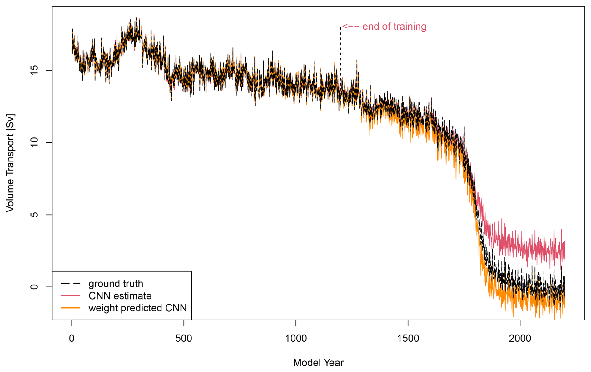
Figure 3 As Fig. 1, but with a sub-optimal example of child model performance. Still, the predicted child model (orange) outperforms the parent model (red) beyond the EOT threshold in the RMSE sense.

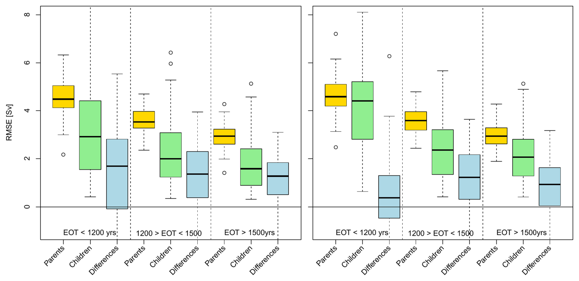
Figure 4 Impact of EOT on the RMSE of a fixed application range (1800 years, 2000 years]. Polynomials of order 1 (left panel) and order 2 (right panel) were fitted to the leading 4 principal components of the input variable (i.e., the meridional velocity maps). Yellow Boxes: RMSE of parent models. Green Boxes: RMSE of child models. Blue Boxes: Pairwise RMSE differences (i.e., unperturbed “parent” model minus corresponding weight-predicted “child” model). Positive values represent improvements due to the presented weight-prediction approach. Each box is based on 100 parents/children/pairs.

Figure 4 is based on the same results as Fig. 2, but here the RMSE are sorted by EOT. In addition, the figure shows only the RMSE for the tipping and the past tipping period. While in the view of Fig. 2, the polynomial of order 1 and order 2 based regressions did look very similar, here in Fig. 4, some large differences become evident. If trained only very far from the tipping point, the regression based on higher-order polynomials leads to wrong results. This strengthens the argument for the fail-mechanism already described, i.e., that higher-order terms get noise-based gradients assigned to them as they are not varying significantly during training and regression. When they then do start to vary during tipping, they will give large yet wrong contributions to the weight prediction, and this way will deteriorate the child model and its output.

In general, the skill of all models (parents and children) improves with larger EOT. This is not only due to more training data per se, but rather that the training data then also includes information located closer to the tipping point. Consequently, the models that are trained up-until tipping perform best, i.e., all yellow boxes go down from left to right in each panel of Fig. 4. On average, even as children and parents show increasingly similar performances with EOT closer to the tipping point, the on average better RMSE of the child models are never reached by the parent models.

A note on temporal data: In experiment 1, we shuffle the training data before applying the training/validation split. In some problems, this is not possible, either due to the choice of architecture (as LSTM) or not advised due to correlations within time (e.g., Schnaubelt, 2019; Bergmeir et al., 2018). If data shuffling is not an option but a test/validation split is still necessary, then the training data is pushed even further away from the tipping point by the presence of the validation window. As a result, the parent models will show an even worse performance. Consequently, our weight-prediction approach will become more advantageous as it also uses the validation data located closer to the tipping point for the weight-regression.

4.2 Experiment 2: Estimation of Sea Water Density

Notable deviations in experiment 2 from the recipe given in Box 1:

• Quantile approach to sample only a fraction of the training data set 𝕀 in step 2a

• No regularization towards 𝕀 is applied during the fine-tuning step 2a (epochs are limited to 4)

• NN inputs (S, T, P, ϕ, λ, and z) are used as weight predictors as well

The NN of choice here is a simple two-layer feed-forward NN with ELU activation functions in the first layer and linear activation in the final layer. The regression of the NN weights uses the same set of variables as the NN input, i.e., S, T, P, ϕ, λ, and z (cf. Sect. 3.2). For the forgetful online learning (Box 1, step 2a), we fine-tune the parent model only on individual x_i without the regularization towards the entire training data set 𝕀. The parent-to-child model differences (ΔW_ik) were limited by limiting the fine-tuning iterations (here: epochs =4) only.

In experiment 2, the training data set is very large, and thus retraining the parent model on every training data point is prohibitively expensive. A random sub-sampling of the training set could lead to undersampling with respect to some of the predictors if the random draw is not sufficiently large. To be efficient and at the same time avoid undersampling the predictors, we sort the training data into quantiles (e.g., 300) for every predictor. Then we draw several x_i from every parameter-specific quantile interval for fine-tuning the parent model (Box 1, step 2). If it is suspected that special functions (or interactions) of predictors should play a role in the weight-regression, then sampling quantiles of the respective function-values (or interactions) is advised (e.g., one has not only to guarantee sufficient sampling of the predictors x and y, but also of log (x), y², and x⋅y etc.).

As in experiment 1, individual ChildModel_a are generated for every single application data point x_a, here, every grid point of the 3d ocean grid.

Figure 5 shows the impact of the weight-prediction approach on a spatial OOD problem, where the parent model is only trained above the dashed line at 2000 m.

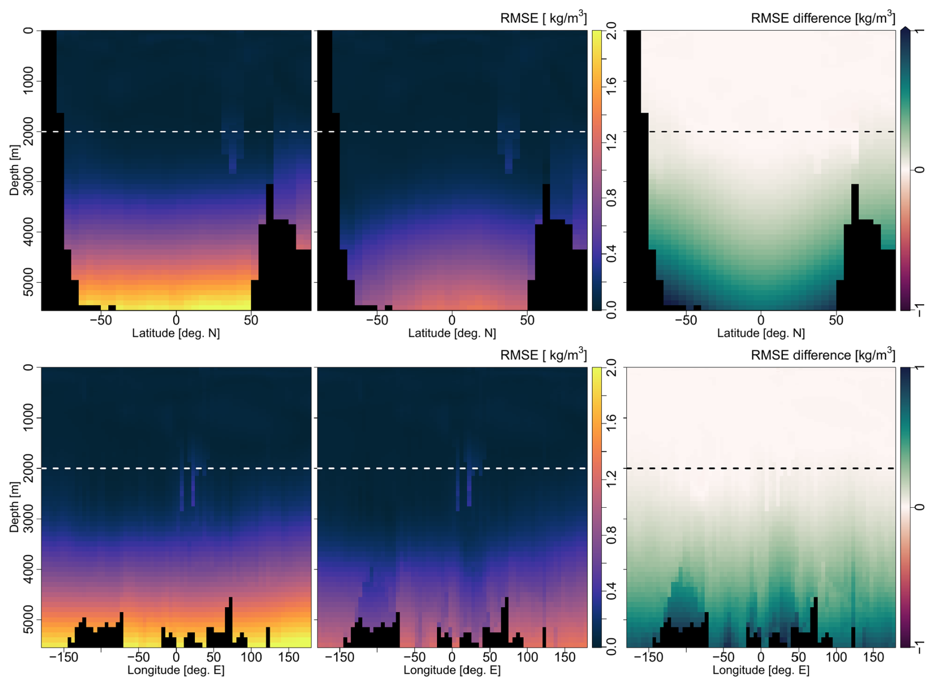
Figure 5 Depth-dependent zonally-averaged^* (upper panels) and meridionally averaged^* (lower panels) RMSE of NN-based sea water density estimation after training above the dashed line only. Left panels: Performance of the parent model. Middle panels: Performance of weight-predicted child model. Right panels: RMSE differences (parent minus child; the green color represents improvements by the child model). ^*: In giving every global output location equal weight, these averages represent a data-centered view and do not follow oceanographic standards.

As a result, the weight-prediction approach improves the performance of the NN sea water density calculation in the deep ocean considerably. At depth, the improvements amount to 2 kg m⁻³ in the global average, which is substantial by oceanographic standards. Below the EOT of 2000 m, the child model improves the RMSE of the parent model by 50 %–100 %. Regions where the parent model already performs well show less or no improvement. As already discussed in experiment 1, even slightly worse RMSE can be found if the approach is applied to the training data. In contrast to experiment 1, the results of experiment 2 appear to be very stable (not shown).

4.3 Experiment 3: Uncertainty Estimation of Global Wind Velocity Reanalyses

Notable deviations in experiment 3 from the recipe given in Box 1:

• A single NN is used instead of several RegressionModel_k in steps 3a & 4a

• Only the final layer of ParentModel₀ is changed to generate the ParentModel_i and ChildModel_a

• EOF of the ParentModel₀ inputs are used as weight predictors

As outlined in Sect. 3.3, this experiment assesses the proposed weight-prediction framework in the context of global wind velocity uncertainty estimation. The focus is on evaluating whether knowledge about uncertainty characteristics learned at one oceanic location can be extrapolated to terrestrial regions with different atmospheric dynamics. This task represents a demanding OOD test case for the proposed method.

Unlike the previous experiments, the child model generation (cf. Box 1, steps 3 and 4) is conducted by a NN, too. This choice of a NN-based child model generation underscores the significance of the underlying weight-prediction methodology over the regression model choice. The child model generation is implemented as a NN consisting of two fully connected hidden layers with 32 nodes each and parameter-specific output heads. Instead of predicting all network weights and biases of the child model, we restrict the weight-regression and prediction to the final fully connected layer, while keeping the remaining parameters identical to those of the parent model. For this to work correctly, the not-to-be-predicted weights and biases have to be set as trainable=FALSE already during the online-learning step (Box 1, step 2). The use of multiple output heads, together with a scaled mean-squared-error (MSE) loss, mitigates scaling disparities across the predicted weights and biases. All layers use ELU activation functions, and the Adam optimizer (learning rate = 0.001) is used.

The training and evaluation periods span 2012–2017, using six-hourly data of the 10 m zonal wind component, from two reanalysis products (ERA5 and CFSv2, cf. Sect. 3.3). Data from 2012–2016 are used for training, January–June 2017 for validation, and July–December 2017 for testing. All results reported below correspond to this testing period. From each of the two input data sets, the principal components of the four leading EOF, yielding eight predictor values in total per time step, are used as weight-regressors. For the regularization of the forgetful online learning (Box 1, step 2a), n is set to 200. The parent model is trained at a single oceanic grid point located at 180° E, 60° S, while the child model predictions are evaluated over the entire landmass to assess the method’s ability to generalize beyond the training regime. As in the other experiments, individual ChildModel_a are generated for every single application data point x_a, that is, every grid point of the 2d globe.

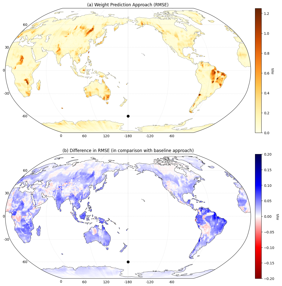
Figure 6 Spatial distribution of RMSE in the prediction of zonal wind-speed uncertainty using the proposed weight-prediction framework. (a) RMSE of the child model trained at the reference oceanic location (180° E, 60° S), represented by the black dot. (b) Difference in RMSE between the parent model and the child model. Blue regions indicate improvements.

Figure 6 summarizes the spatial distribution of the RMSE in zonal wind speed uncertainty prediction. Panel (a) shows the RMSE obtained by the child model trained only at the oceanic reference point (black dot), and panel (b) illustrates the parent minus child model RMSE differences. Blue areas in Fig. 6b mark regions where the proposed method outperforms the parent model, i.e., where RMSE are reduced by the weight-prediction method.

From these results, it is evident that the weight-prediction approach substantially enhances the wind velocity uncertainty estimation over continental regions, particularly where the parent model struggles the most. Notable improvements are observed over the southeast coast of Australia, eastern Brazil, the East African Highlands, the Indonesian archipelago, and southeastern Russia. In contrast, regions where the parent model already performs well show no major improvement, as expected. This applies to most of the oceanic region as well (not shown in the figure). This behavior suggests that the proposed method provides the greatest benefit under conditions of strong distributional shift, where the parent model’s learned representations are least transferable (cf. experiments 1 and 2).

Quantitatively, the terrestrial global mean RMSE of the uncertainty estimates decreases from 0.1236 to 0.1104 m s⁻¹, corresponding to an average improvement of approximately 10.7 %. Repeated experiments indicate that this value varies between −2 % and 14 %, with a mean improvement of 5.25 %, reflecting again the stochastic variability inherent in NN training. Despite this variability, the consistent tendency across repeated experiments confirms that the proposed method systematically improves the predictive performance of the parent model, particularly in regions where generalization is most challenging.

That a NN can be used to improve the OOD problem of another NN seems contradictory at first. Overall, the terrestrial input is equally OOD to the ParentModel₀ as well as to the child-generating NN. One could ask why the child-generating NN is not limited by OOD, and why then not one NN alone can handle the problem. A full answer to these questions remains open to further research. So far, we can only argue that we, as users, know if an OOD task we gave to a NN remains generally the same but has to be adapted to perform outside the training realm. Consequently, splitting an OOD-experiment into problem-solving and problem-adaptation represents a form of structural implementation of prior knowledge. This understanding, the required task separation, and the subsequent training of both NN, a single NN cannot (yet) develop itself. Furthermore, as already discussed, a nonlinear regime shift in a NN's input and output data can be less nonlinear in the weight-space of the same NN when nonlinear activation functions are involved.

5 Summary and Final Remarks

In this study, a general method is presented that aims at improving neural network (NN) performance outside of their training data distribution (OOD). The method is proposed for problems where NN are used for one of the various reasons and re-normalization or standardization of the inputs or outputs is not possible due to limited data in few-shot problems or due to governing nonlinear relations, e.g., in climate sciences. Additionally, OOD is meant in a wider sense here. Even when all input variables have the same distribution within and out of training, a trained NN can operate on uncharted territory due to unseen value-combinations and interactions of the input variables.

After the training of a NN, which we call “parent model”, on a specific problem, the method requires the following three steps: First, the method collects the series of weight anomalies that arise by online-relearning or fine-tuning of the parent model towards subsets of the training data. Second, a relation (e.g., a linear regression) is to be established between these weight anomalies and suitable predictors (e.g., the input variables of the training data set itself). Third, the established relation is then used to generate new weights and thus a new NN that corresponds to an application data set by employing the same predictors but now with values that correspond to the application data set (e.g., the application data itself). In analogy to the parent model, we call this new model the “child model”. A child model can encompass a group of NN as a new NN can be generated for every single application data point (time step or location). However, sub-setting is possible in all steps of the approach. For example, only one new NN could be generated per cluster of the application data set. Likewise, the weight sensitivities could be derived from quantiles or clusters of training data only.

Note, reasonable choices for the mentioned subsets should depend on the self-similarity the training data, respectively, the application data has. For example, if the training data shows notable clusters, fine-tuning on these clusters should be sufficient. Furthermore, if the application data is rather homogeneous, one does not need to calculate a single child model for every application data point.

In short, the approach is generating NN fine-tuned on subsets of the training data and then is extrapolating along these NN to data-regions outside of the training data distribution. This way, the network's learned tasks can be transferred, e.g., to different geographic locations, future climates, or across (physical) regimes.

The method is demonstrated on 3 very different examples from Earth sciences: one temporal problem, one spatial problem, and one spatiotemporal problem. These examples and their execution demonstrate further the possible flexibility of the core approach in using linear, nonlinear, and NN-based regression methods; full and partial NN weight prediction; and different realizations of the online training step and its regularization.

In summary, our experiments demonstrate that the proposed weight-prediction framework enhances the extrapolation capability of NN under strong temporal, spatial, and regime shifts. The method proves most effective where traditionally trained and therefore static models exhibit limited skill, underscoring its potential to extend NN capabilities to previously unseen regimes and conditions. As a result, NN can become adaptive and more dynamic operators.

Despite all these promising results, there are still some caveats, as choices have to be made that can heavily impact the method's performance. The choice of suitable predictors, e.g., if one does not choose the input variables themselves, has to be based on prior knowledge. This should pose no major problem for the experienced researcher. The same can be stated about the choice of whether all weights and biases of a NN or only specific subsets should be subjected to weight-regression and subsequent weight-prediction.

In contrast to these rather straightforward choices, the choice of the weight-regression and prediction method cannot be based on prior domain knowledge alone. The reason is that the weight sensitivities the proposed approach has to model are entwined with the network architecture and the employed activation functions. As a first guide, linear or slightly nonlinear regression methods should work fine for most cases.

The biggest drawback identified so far is that the weight-prediction method has inherited the notorious stochastic nature of NN training. From several parent NN (with identical architecture and hyperparameters) that are trained on the same data, not all produce better-performing offspring. To this issue, the most follow-up research will be dedicated. Although we already discussed possible reasons and solutions within the manuscript, we will have to understand the problem better to be able to identify and select parent models suitable for weight-regression or, in the long run, even foster the generation of more suitable parent models through adapted training procedures. Additionally, we see much room for improvement in the generation of the child models by predictor pruning, weight-regression validation, regression-ensembles, transformers, or other means.

As a conclusion, most steps of the approach may be called more or less experimental and can and will be improved in follow-up research. However, already now the method has to be considered very promising and is at least in our experiments robust in the ensemble-average sense.

As a further outlook, we see this method also as a promising tool for NN applications without OOD. During our many tests, we got the impression that the method can improve the performance of undertrained, overfitted, or by design under-complex models as well.

Despite the fact that all given examples are from Earth sciences, the authors strongly believe that the demonstrated approach is useful in other fields, such as astrophysics, biology, social sciences, or technical applications. For example, in medicine, the approach could be used to transfer learned skills and knowledge to patient groups underrepresented or unrepresented in the training data.

Appendix A

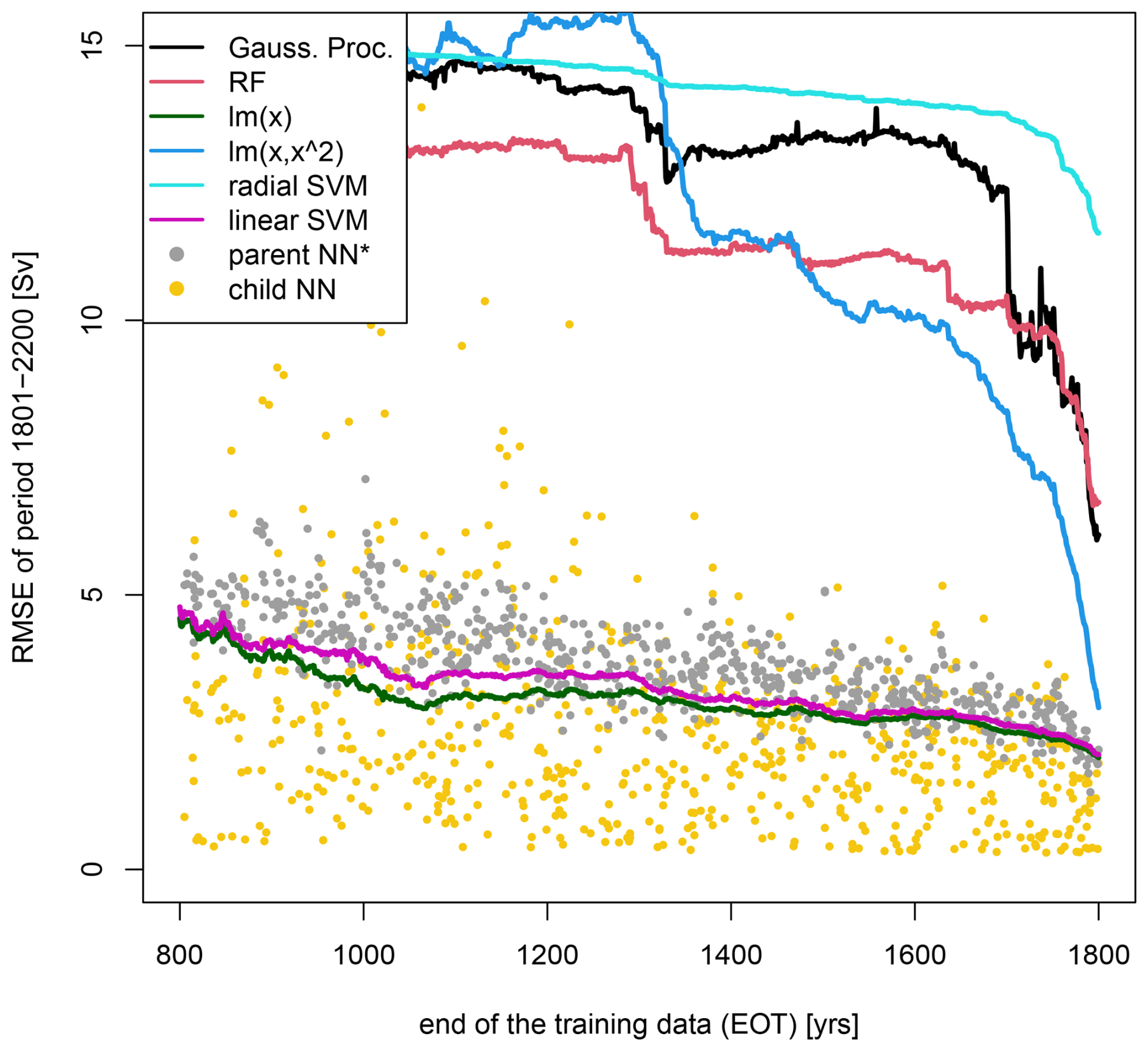
Figure A1 Performance comparison of parent and child NN to non-NN extrapolation methods in experiment 1. Impact of EOT on the RMSE of a fixed application range (1800 years, 2000 years]. Lines show non-NN approaches: Gaussian processes (linear predictors), random forest (linear predictors), linear regression (linear predictors), linear regression (linear and squared predictors), linear and radial kernel SVM (linear predictors) are fitted to the leading 4 principal components of the meridional velocity maps. Dots show the parent NN and linear-fit-based child NN (cf. Fig. 4). ^* Note that the parent NN base their AMOC strength estimates on the velocity fields only, and not on the principal components, as the other methods do, i.e., the NN have to learn a suitable representation themselves, while the other methods benefit from prior knowledge.

To provide a baseline, we present and compare a range of standard linear and nonlinear methods used to extrapolate the targets of experiments 1 and 2, i.e., AMOC strength and sea water density, without any use of NN. The methods (Gaussian process, linear model, random forest, and support vector machine) were fitted to the same predictors as the weight prediction method, i.e., 4 leading EOF (experiment 1) and S, T, P, ϕ, λ, and z (experiment 2). Likewise, the respective OOD projections are based on the same predictors that our weight prediction method uses. Note that none of these methods outperform the child models in the OOD application cases. Most of the methods do not outperform the parent NN (ParentModel₀) either. However, even if a method exists that outperforms both the parent and the child NN in our specific use cases, our approach remains useful in all cases where NN are used for one of the various reasons, e.g., ease of use and implementation, existing NN workflows, compute limitations, invertibility requirements, or simple lack of alternatives (e.g., decision making, generative AI, image classification).

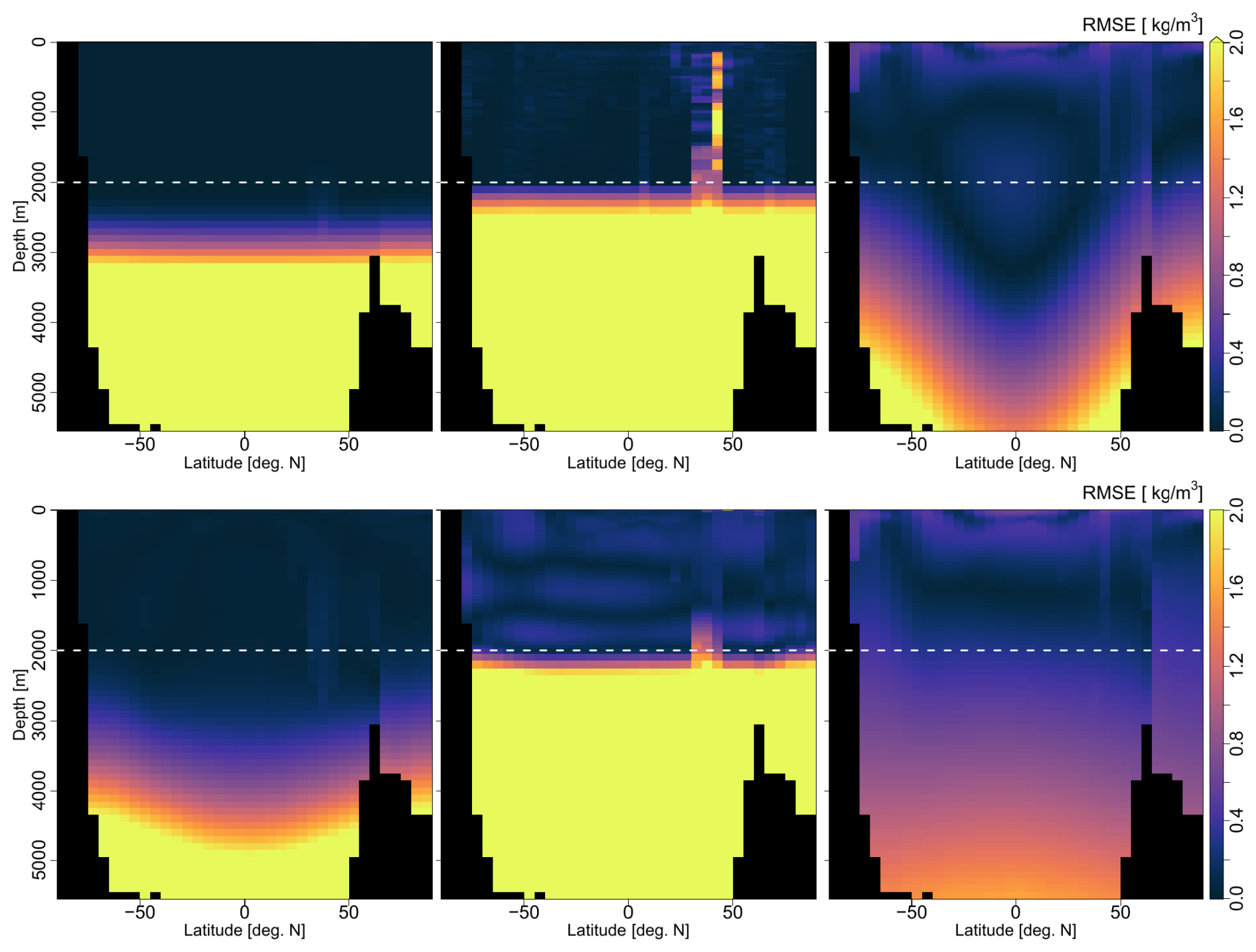
Figure A2 Non-NN model performance of experiment 2 (cf. Fig. 5, upper panel). Depth-dependent zonally-averaged^* RMSE of non-NN sea water density estimation after training on ground truth data above the dashed line only. Upper row: Gaussian processes (linear predictors), random forest (linear predictors), linear regression (linear predictors). Lower row: Linear regression (squared predictors), radial kernel SVM (linear predictors), linear kernel SVM (linear predictors). Predictors in all cases are S, T, P, ϕ, λ, and z (cf. Sect. 3.2). ^* In giving every global output location equal weight, these averages represent a data-centered view and do not follow oceanographic standards.

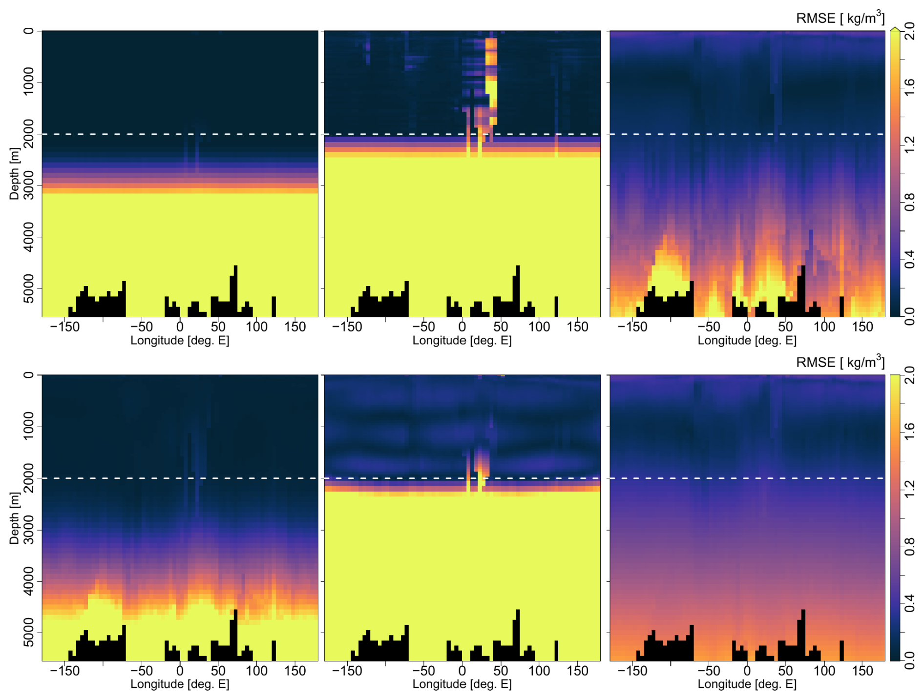
Figure A3 Non-NN model performance of experiment 2 (cf. Fig. 5, lower panel). Depth-dependent meridionally-averaged^* RMSE of non-NN sea water density estimation after training on ground truth data above the dashed line only. Upper row: Gaussian processes (linear predictors), random forest (linear predictors), linear regression (linear predictors). Lower row: Linear regression (squared predictors), radial kernel SVM (linear predictors), linear kernel SVM (linear predictors). Predictors in all cases are S, T, P, ϕ, λ, and z (cf. Sect. 3.2). ^* In giving every global output location equal weight, these averages represent a data-centered view and do not follow oceanographic standards.