Covariations between persistent synoptic features and record low Antarctic sea ice events via unsupervised regression learning

During the past decade, a succession of record low sea ice events has led to the suggestion that a shift in the overall dynamics of sea ice in the Antarctic region is underway. We attempt to gain fresh insight into how persistent atmospheric states may play a role in these anomalous events, particularly their influence on Antarctic sea ice retreat in the warmer months, by studying coupled atmosphere-sea ice variability during the 2016–2017, 2021–2022, and 2023 low sea ice concentration years. We construct a reduced-order model from reanalyzed observations based on a well-developed machine learning algorithm incorporating coupling across subsystems, namely the atmosphere and sea ice. Background persistent events occurring throughout the years of interest are then extracted via non-stationary transition matrix methods to the resultant temporal sequence of states. These events are analyzed by considering the associated surface pressure, winds, temperature, and sea ice concentration. The results show that persistent patterns in the atmosphere covary with the rate and spatial patterns of sea ice growth and retreat, noting that some periods of retreat coincide with warm surface temperatures and relatively quiescent synoptic winds. Our non-stationary approach provides additional insight over and above what can be inferred from simple monthly or seasonal averages alone, particularly in capturing events across varying temporal scales.

1 Introduction

The Antarctic region experienced an overall net increase in sea ice between 1979 and 2015 (Parkinson and Cavalieri, 2012; Stammerjohn et al., 2025). However, more recently, unprecedented record low sea ice extents have occurred in the 2016–2017 and 2021–2022 Austral summers and the 2023 Austral winter (Espinosa et al., 2024; Schlosser et al., 2018; Scott, 2023; Stammerjohn et al., 2025; Stuecker et al., 2017; Suryawanshi et al., 2023; Turner et al., 2017; Wang et al., 2019, 2023). These extreme levels have led some to argue that this is indicative of a long-term qualitative change in the sea ice dynamics of the Antarctic region (Eayrs et al., 2021; Purich and Doddridge, 2023; Hobbs et al., 2024). The emerging literature concerned with this phenomenon has investigated several possible drivers in the atmosphere (Schroeter et al., 2023) and ocean (Narayanan et al., 2026) together with a consideration of the role of anthropogenic forcing behind the recent changes (e.g. Morioka et al., 2024).

In this study we apply nonstationary clustering and Markov transition methodologies to reanalysis data with a focus on identifying the role of persistent large-scale atmospheric events during recent years where record low sea ice extent has occurred. Previous work has suggested various atmospheric patterns that might underpin anomalous low sea ice events; these include the zonal wave-3 pattern (ZW3) (Schlosser et al., 2018), the southern annular mode (SAM) (Gurjão et al., 2025; Schlosser et al., 2018; Stuecker et al., 2017), the Pacific-South American patterns (PSA) (Gurjão et al., 2025), a general warming pattern over the Antarctic (henceforth called the Antarctic warming pattern) as described in Franzke et al. (2015), and the Amundsen Sea Low (ASL) (Wang et al., 2023; Yadav et al., 2022). These mid- to high-latitude atmospheric modes of variability and their teleconnections are dynamical processes that regulate the winds at low-lying latitudes which in turn affect the development of sea ice e.g., the poleward transport of warmer, tropical air through mechanisms such as the ASL (Holland et al., 2018). The degree to which these states persist as localized stationary patterns further induces thermodynamic responses in the sea ice due to advection of surface heat fluxes.

We base our study on three recent years: 2016–2017, 2021–2022, and 2023 using reanalysis datasets that incorporate covariations between the atmospheric precursors and subsequent record low sea ice extent and for which diverse atmospheric patterns have been attributed to each of these particular events. The year 2016 has been previously described in terms of a persistent positive zonal wave-3 (ZW3) index between May and August, a low monthly mean SAM index in November, and a deepened ASL in September (Schlosser et al., 2018; Stuecker et al., 2017; Turner et al., 2017). All of these processes, when combined with ocean-based teleconnections including the El-Niño Southern Oscillation (ENSO) (Stuecker et al., 2017), created conditions that arguably led to the major low sea ice event in 2017. By way of contrast, the year 2021 was characterized by a deep ASL event throughout October and November (Turner et al., 2022; Wang et al., 2023). Finally, the 2023 record low sea ice event contrasts further by occurring throughout the austral autumn and winter (Ionita, 2024; Josey et al., 2024).

Many of the aforementioned studies employ methodologies that are either stationary in nature or averages over uniform fixed periods (e.g. months), and hence are not suitable for an analysis of heterogeneous metastable events. Some studies use statistical analysis methods such as the F-test, t-test, and change-point detection strategies to determine whether the low events were statistically significant or attribute the event to the pattern that is associated with the low (Hobbs et al., 2024; Ionita, 2024; Purich and Doddridge, 2023). Such methods are statistically stationary and focus more on long-term shifts than short-term variations. Time-evolving statistical methods have also been attempted, such as that described by Maierhofer et al. (2024) where a vector-autoregressive moving average model is applied to a Bayesian framework for sea ice reconstruction. Others have considered the effect of various climate indices relevant for the Antarctic such as the SAM index (Goyal et al., 2021; Gurjão et al., 2025; Schlosser et al., 2018; Suryawanshi et al., 2023; Turner et al., 2017; Wang et al., 2019, 2024), but these indices are typically on monthly or seasonal timescales, which leaves short events associated with particular synoptic patterns vulnerable to being averaged out or cut off due to temporal boundaries. While various ocean and climate general circulation model frameworks such as the CMIP series have been used to simulate conditions and recreate factors behind recent events (Espinosa et al., 2024; Gao et al., 2021; Goyal et al., 2021; Morioka et al., 2024; Stuecker et al., 2017; Wang et al., 2024, 2023; Narayanan et al., 2026) these are limited by model resolution, biases and a paucity of subsurface observations in the sea ice zone. More generally, the high dimensionality and non-stationarity of reanalyses and model data renders the isolation of mechanisms important to given persistent anomalous events particularly challenging.

The majority of the aforementioned studies average data over fixed temporal boundaries, often weekly, monthly, seasonal or annual measures. In this work we adopt a somewhat different strategy. After determining a sequence of daily data affiliations to non-stationary cluster states via a time-dependent vector autoregressive model optimised to the full reanalysis dataset, we consider individual background events of variable length (minimum of 10 d (days), ranging up to over two months) via application of Markov transition matrices. This approach enables us to examine the events of a given year in a way that the imposition of prescribed temporal boundaries cannot. This flexibility facilitates the consideration of short, yet potentially impactful, events whose significance might be lost if the event were to be averaged out over an imposed longer time period. Furthermore, this allows us to identify any events that might span arbitrarily placed temporal boundaries that otherwise risk being missed by stationary methods. Our technique is an example of a non-stationary approach to a non-stationary problem. By allowing the temporal boundaries to be defined by the events themselves, rather than being decided a priori, we identify key persistent events in a systematic way which is sufficiently adaptable to reflect their inherent underlying variability.

Using methods rooted in clustering algorithms, specifically the Finite Element Method Bounded Variations Vector Autoregressive (FEM-BV-VAR) machine learning method (Horenko, 2010), in combination with the use of multivariate singular value decompositions (SVD), we generate reduced-order models that describe how the concentration in sea ice varies with changes in the atmosphere. This approach allows extraction of the underlying background states for various cases, and identification of impactful persistent synoptic structures present in the lead up to the low sea ice events. Previous studies have demonstrated the utility of the FEM-BV framework in analysing climate modes of variability (Horenko, 2010; O'Kane et al., 2013b; Franzke et al., 2015; Quinn et al., 2021; Axelsen et al., 2025). In particular, O'Kane et al. (2013b) used the FEM-BV-VAR approach to analyze a set of coupled ocean-sea ice simulations that reveal significant changes in the meta-stability of the Southern ocean dynamics and sea ice concentrations around Antarctica in response to changes in atmospheric forcing from the early 1980s. They detected regional dependencies in sea ice concentrations that arose due to specific combinations of random stochastic, high-frequency weather, seasonal, and interannual atmospheric forcing. In this study, transitions between locally stationary metastable states identified using FEM-BV-VAR are further modelled using discrete-time Markov chain transition matrices. While Markov models have previously been used to attempt to forecast Antarctic sea ice (Chen and Yuan, 2004), we instead use them to find the prominent background state over periods of time. A major motivation for this study is to utilize non-stationary time-series methods to facilitate better understanding of the combined thermodynamic and dynamical processes associated with major atmospheric modes of variability in the context of record low Antarctic sea ice events.

The rest of the paper is structured as follows. In Sect. 2, we describe the approach for extracting persistent events in the coupled atmosphere-sea ice system. In particular we discuss the data selection, clustering method, and the Markov model. Next, in Sect. 3, we analyze the three chosen years and the events that occur within them. We close in Sect. 4 with a synthesis of the results and provide an outlook for future work. Methods are detailed in Appendix A with correlations between local cluster states and atmospheric teleconnection patterns included in Appendix B.

2 Data and Methodology

2.1 Datasets

We use the NCEP-NCAR Reanalysis Project Reanalysis 1 (NNR1) daily mean datasets for this study (Kalnay et al., 1996). To determine the optimal model, we consider covariations between troposphere and sea ice using geopotential height datasets at the upper, middle, and lower troposphere (200, 500, and 850 hPa) alongside sea ice concentration for fitting a reduced-order model. We also consider geopotential height, air temperature, and the u- and v-winds all near the surface (1000 hPa) as diagnostics over the period between 1 January 1959 and 31 October 2024. We restrict ourselves to the Southern Hemisphere (latitude between 0 and 90° S) and remark that each level of data has a spatial resolution of 2.5° × 2.5° in latitude and longitude. In total then, we have 73×144 data points for each of the 24 046 d. The sea-ice dataset, however, was structured in a slightly different, latitude-varying format (1.83–1.9° lat × 1.875° lon); when required, we use a Python linear re-gridding process to ensure compatibility with the other datasets. Finally, we also considered the sea ice extent (SIE); this is defined to be the total area where the sea ice concentration (SIC) exceeds 15 % (Scott, 2023). Specifically, from the raw concentration data a filter is applied (i.e., if SIC > = 0.15, then 1, otherwise 0), after which anomalies are calculated with respect to the daily climatological mean (1 January 1979–31 October 2024). Following that, a linear regridding process (xarray.regrid.linear) is applied (along with a conversion to the latitude-longitude format from stereographic projection for the NSIDC dataset) to regrid both anomaly datasets onto a common uniform 2.5° × 2.5° grid in latitude and longitude. We then take the average extent anomaly for that day/month over every grid point (where the anomalous SIE value is not 0 or NaN using numpy.mean) to get the daily/monthly average SIE anomaly per grid point.

We note that the dataset we use from NNR1 includes 20 years of pre-satellite observations. The inclusion of these additional decades ensure that there is a sufficient number of samples for the model-fitting procedure. The fidelity of some of the pre-satellite data has been questioned (e.g. Kistler et al., 2001 discusses some of the errors in the 1959–1978 period that have been fixed) and in an effort to assess the importance of this, we compared our full results against those derived using only satellite-era information. To test the robustness of the NNR1 sea ice concentration reanalysis relative to direct observations, we adopt the National Snow and Ice Data Center (NSIDC) sea ice concentration dataset as a reference point (Meier et al., 2024).

A comparison between the reanalysis and the observed data in Fig. 1 shows that over the satellite record, and particularly during the years relevant to this study, the two datasets exhibit small differences in anomalies for sea ice concentration and extent with the same general trend, but that the NNR1 dataset leans more conservatively with respect to negative anomalies after 2015. We also note that NSIDC currently uses NNR1 for assessments of atmospheric circulation and temperature. On that evidence, we assume that NNR1 is a sufficiently reliable and consistent dataset to base our study. Reassuringly, we found no significant change in the root mean square error (RMSE) of the optimal model class when fitting reduced order models to the full reanalysis period or only over the satellite period, thus we retain the additional decades for the subsequent analysis. That said, and regardless of choice of reanalysis, biases will be present (e.g., Bromwich et al., 2024 report major artifacts in ERA5 2 m air temperature trends over Antarctica prior to and during the modern satellite era). Goodwin et al. (2026) note substantial differences in respective simulations of the 2023 Antarctic sea ice record minimum using a coupled ocean–sea ice model (NEMO-SI3) forced by either ERA5 and JRA-55-do reanalyses.

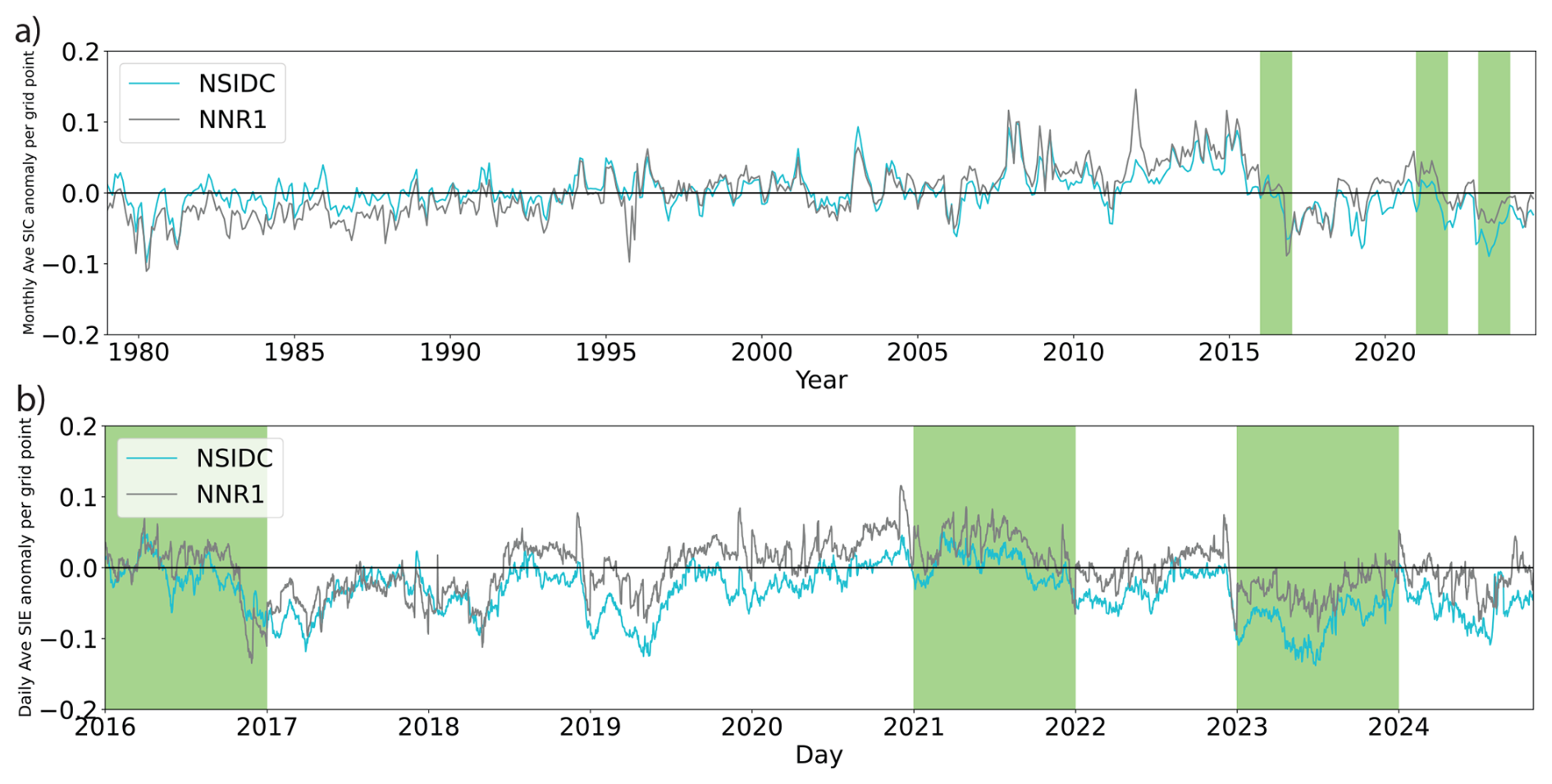
Figure 1 (a) A time series of monthly average anomalies in Antarctic sea ice concentration per grid point since 1979 in the Southern Hemisphere (assuming a 2.5° × 2.5° resolution) for the NSIDC and NNR1 datasets. Data was converted (where appropriate) to latitude-longitude format, and then regridded to the given resolution using a linear interpolation method. (b) Time series of daily average anomalies in Antarctic sea ice extent per grid point over the years post 1 January 2016 to 31 October 2024. Shaded in green are the time periods considered for the study.

2.2 Determination of the reduced-order model

We determine a reduced-order model from a given set of data using a process similar to that described in Axelsen et al. (2025). The key elements are described here with further details in Appendix A. To start, we first apply a weighting of $\sqrt{\cos \mathit{\alpha }}$ to the data, where α is the latitude. After the daily climatological mean, calculated over the period between 1 January 1959 and 31 October 2024, has been removed, we employ a principal component analysis (PCA) performing a multivariate singular value decomposition (SVD) on the 850, 500, and 200 hPa geopotential height and sea ice concentration anomaly datasets. These datasets are normalized to have unit matrix norms on each level and day, and interpolated to a common grid prior to performing the SVD. This allows for an equal contribution between sea ice concentration and tropospheric geopotential height anomalies for the PCA outputs expressed as a linear combination of principal components (PCs) and empirical orthogonal functions (EOFs). Specifically, the PCA is performed on the stacked, normalized dataset D through the equation

$$\begin{array}{}\text{(1)}& D=XS{V}^T,\end{array}$$

where X=[x_t] are the PCs, S represents the singular values that denote how much of the explained variance can be attributed to each PC/EOF pair, and V^T gives the multi-dimensional EOFs. For the given hyperparameter choices we then supply the leading 20 PCs to the FEM-BV-VAR learning algorithm. This number of PCs explains 56 % of the total variance, sufficient to capture variability relevant to the major blocking and synoptic-scale features while reducing the dimensionality sufficient to obtain convergence in the optimization and avoid overfitting.

Hyperparameter ranges are chosen corresponding to characteristic e-folding times for synoptic flows:

• $K\in \mathit{\{}\mathrm{2},\mathrm{3},\mathrm{4}\mathit{\}}$ – the number of clusters (metastable states in the model),

• $m\in \mathit{\{}\mathrm{3},\mathrm{4},\mathrm{5}\mathit{\}}$ – the memory length (the number of lags in the VAR model), and

• $p\in \mathit{\{}\mathrm{0},\mathrm{1},\mathrm{\dots },\mathrm{6},\mathrm{7}\mathit{\}}$ – the average level of persistence. This regulates how many transitions between clusters a model can make, with higher values of p implying fewer transitions.

From the FEM-BV-VAR process, we obtain an optimal set of parameters for the VAR model and an affiliation sequence that assigns a probability of a given data instance to reside in one of K locally stationary cluster states. The optimal model for a prescribed set of hyperparameters is determined by minimizing the RMSE. This requires cross-validation; models are tested on a training dataset and iterated until ten folds have occurred sufficient to ensure that the model has converged to its minimal RMSE (Friedl et al., 2002; Twomey and Smith, 1997). An expanded description of the FEM-BV-VAR algorithm and cross-validation method is described in Appendix A.

Considering all 72 combinations of hyperperameters, the minimum mean RMSE is achieved when $(K,m,p)=(\mathrm{4},\mathrm{5},\mathit{\{}\mathrm{0},\mathrm{1}\mathit{\left\}}\right)$, as shown in Fig. 2. Choosing p=0 or p=1 effectively assumes no upper bound on transitions resulting in equivalent results (Axelsen et al., 2025). For this study we find $(K,m,p)=(\mathrm{4},\mathrm{5},\mathrm{0})$ to be our preferred model i.e., a 5th-order VAR model with 4 metastable states and no enforced persistence. Restricting the time period range to only the satellite era we observe little difference in the optimal model RMSE however, time periods significantly shorter than the satellite period (e.g., 2010–2024) will have a larger effect of the optimal model class, with the reduced sample sizes resulting in lower confidence and increased potential for overfitting. Previous studies have revealed cross-validation as a less restrictive approach to model selection. In particular, information-theoretic approaches such as Akaike's information criteria can over-penalize for the number of clusters K (O'Kane et al., 2013a).

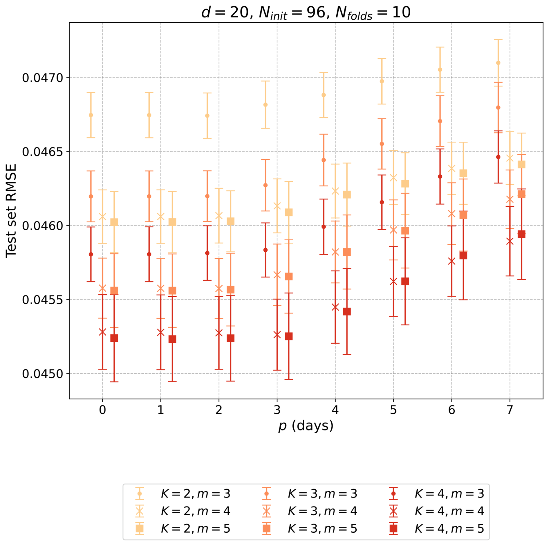
Figure 2 The root mean square error (RMSE: Eq. A8) for all 72 combinations of hyperparameters tested up to k=4 where the bars indicate the error bounds. The optimal class of models corresponds to K=4 and m=5, with p=0.

Key to the following analysis is the derived affiliation sequence $\mathrm{\Gamma }\left(t\right)=\left[{\mathit{\gamma }}_{\mathrm{1}}\right(t),\mathrm{\dots },{\mathit{\gamma }}_K(t\left)\right]$ where γ_j(t) denotes a convex non-negative probability value with the constraint that ${\sum }_{j=\mathrm{1}}^K{\mathit{\gamma }}_j\left(t\right)=\mathrm{1}$ for all t to other variables such as temperature and the zonal and meridional winds. The process we use to derive Γ(t) is given in Appendix A.

2.3 The background events

Having obtained the daily affiliations Γ(t), we extract a binary sequence or Viterbi path k_t; this is a sequence that identifies the state taken by the reduced-order model on any given day. The preferred state is the one with the highest affiliation rating, defined by

$$\begin{array}{}\text{(2)}& k_t:=\underset{j}{max}\left({\mathit{\gamma }}_j\right(t\left)\right),j\in \mathit{\{}\mathrm{1},\mathrm{\dots },K\mathit{\}}.\end{array}$$

The Viterbi path enables identification of persistent occurrences of specific metastable states over a defined period. Composites using the original datasets (NNR1 anomalies) over the lifetime of a given event results in a lossless graphical representation of the local metastable state. The Viterbi path allows contiguous sequences of observed anomalies for any variable to be averaged to produce composite patterns for a given event. The coherence and amplitude of the composite pattern is an indication of the persistence of the event and the (un)certainty of its existence. Since the FEM-BV-VAR method output is non-stationary (by construction), the metastable states best reflect temporally local fluctuations in patterns and events that evolve over time. As such, the analysis that follows focuses on short-term composite states.

The characteristic timescale of coherent features in Southern Hemisphere synoptic flow is typically on the timescale of days, which is supported by the persistence of the optimal model. However, in order to identify the slow manifold characterizing the evolution of SIE (i.e., the background state) that preceeds the anomalously low SIE events in our three chosen years, we transform the Viterbi path into an alternative sequence that identifies the “most prominent” cluster state over a given period. That is, the most probable cluster over a defined window. This is accomplished by using a transition matrix method. The following approach of fitting a Markov model to an affiliation time series was described in Crommelin and Vanden-Eijnden (2006), and later applied to an FEM-BV sequence by O'Kane et al. (2013a).

We first create a K×K local transition matrix ${\mathbb{P}}_{t_{\mathrm{0}}}^{t_{\mathrm{1}}}\left(t_{\mathrm{F}}\right)=\left[{\mathbb{P}}_{ij}{]}_{t_{\mathrm{0}}}^{t_{\mathrm{1}}}\right(t_{\mathrm{F}})$ for the period t ∈ [t₀,t₁] where we define

$$\begin{array}{}\text{(3)}& {\mathbb{P}}_{t_{\mathrm{0}}}^{t_{\mathrm{1}}}(t_{\mathrm{F}}{)}_{ij}:=\mathit{Pr}(k_{t+\mathrm{1}}=j|k_t=i),t\in [t_{\mathrm{0}},t_{\mathrm{1}}],i,j\in \mathit{\{}\mathrm{1},\mathrm{\dots },K\mathit{\}},\end{array}$$

where $\mathit{Pr}(k_{t+\mathrm{1}}=j|k_t=i)$ describes the fraction of times the Viterbi path entered state j from state i over the prescribed period. Equation (3) generates a discrete-time Markov chain where t_F is the representative day chosen for the Markov chain over the interval [t₀,t₁]. We take t_F to be the final day in the window. This choice of t_F is important in that different options will translate the resulting sequence from this derivation by a number of days and make the resulting patterns either a reflection of the past, future, or a mixture of both. Furthermore, the local metastable states are not invariant patterns, and thus different choices could identify different dynamics. Reassuringly, we confirm that setting t_F to the first day of the window does not significantly change the results obtained in this study. This contrasts with stationary analyses, in which patterns are often invariant due to assigned temporal boundaries. By setting t_F to be the final day in the window, we are identifying the pattern that is the culmination of the occurrence of a prominent state over that window. We then calculate the local stationary distribution over the interval [t₀,t₁] by solving the matrix equation

$$\begin{array}{}\text{(4)}& {\mathit{\pi }}_{t_{\mathrm{0}}}^{t_{\mathrm{1}}}\left(t_{\mathrm{F}}\right){\mathbb{P}}_{t_{\mathrm{0}}}^{t_{\mathrm{1}}}\left(t_{\mathrm{F}}\right)={\mathit{\pi }}_{t_{\mathrm{0}}}^{t_{\mathrm{1}}}\left(t_{\mathrm{F}}\right),\end{array}$$

for a probability vector π of length K; moreover we need to ensure that ${\mathit{\pi }}_{t_{\mathrm{0}}}^{t_{\mathrm{1}}}(t_{\mathrm{F}}{)}_j\ge \mathrm{0}$ for all j and that ${\sum }_{j=\mathrm{1}}^K{\mathit{\pi }}_{t_{\mathrm{0}}}^{t_{\mathrm{1}}}(t_{\mathrm{F}}{)}_j=\mathrm{1}$. We can then develop a temporal sequence from each of prominent states from the local stationary distributions (denoted P_TM) over each interval [t₀,t₁] using

$$\begin{array}{}\text{(5)}& P_{t_{\mathrm{0}}}^{t_{\mathrm{1}}}(t_{\mathrm{F}}{)}_{\mathrm{TM}}:=\arg \underset{j}{max}({\mathit{\pi }}_{t_{\mathrm{0}}}^{t_{\mathrm{1}}}\left(t_{\mathrm{F}}{)}_j\right),\end{array}$$

where the TM subscript refers to the transition matrix method we use. Care must be taken should either an absorbing or an isolated state occur at some time during the period $t\in [t_{\mathrm{0}},t_{\mathrm{1}}]$ (i.e., when the local transition matrix is not ergodic). This tends to be more common when operating with shorter windows. To deal with this, we first temporarily reduce the upper bound t₁ so that all absorbing states become isolated ones. Then all isolated states post-adjustment are dropped from the matrix equation (4). This allows us to obtain the stationary distribution among all metastable states which the system transitions from over the time period t ∈ [t₀,t₁]. We then repeat this process through a sliding-window approach by incrementing t_F and the window by one timestep until we reach the end of our dataset, creating the π_j curves and sequence P_TM that allows for daily evolution based on the window.

Once the π_j curves and the P_TM sequence are both formed, we apply a locally weighted scatterplot smoothing (LOWESS) method to generate a smoothed curve for each of the π_j , specifically Python's statsmodels.nonparametric.lowess method. The LOWESS method was originally pioneered by Cleveland (1979) as a technique for filtering noise in scatterplots by fitting a smooth curve. We ensure that the LOWESS-smoothed curves follow the assigned π_j as closely as possible by setting the fraction parameter of the function to be the maximum window length $|t_{\mathrm{1}}-t_{\mathrm{0}}|$ divided by the number of days in our full dataset (24 046 d). The smoothed curves are compared with their respective π_j to find the prominent cluster. If, on a given day, both the $P_{t_{\mathrm{0}}}^{t_{\mathrm{1}}}(t_{\mathrm{F}}{)}_{\mathrm{TM}}$ and the LOWESS-smoothed curves suggest that one particular cluster is the most likely state, then we say it is prominent. If the two methods select different clusters we conclude that neither is prominent. This process produces a sequence that allows us to better associate events with particular clusters.

We observe physical manifestations of the most prominent clusters in local time (over a relatively short window) that persist for at least ten days, thereby exploiting the non-stationary properties of the reduced-order models. We set the maximum window length of our method at 30 d ($|t_{\mathrm{1}}-t_{\mathrm{0}}|=\mathrm{30}$). This choice of window length represents a balance between the timescales of the atmosphere (days) and sea ice (seasonal).

To assess the confidence that the extracted patterns are coherent structures, we perform pattern correlations with known teleconnections in the SH region. In the case of an established Amundsen Sea Low (ASL), we also assess the amplitude of the low to establish confidence in “deep” ASL events. The details of this analysis are provided in Appendix B.

3 Results

Here, we apply the methodology described in Sect. 2 to the years 2016, 2021, and 2023. Our results explore each of the precursors for the recent record low Antarctic sea ice events that occurred in the austral summers of 2017 and 2022, and the austral winter of 2023.

3.1 2016–2017 case study

We begin our analysis by investigating the possible precursors for the 2016–2017 austral summer low sea ice event, considering the covariations between atmospheric states and sea ice concentration over the preceding year of 2016. Figure 3 shows ten persistent background events across the year: there are two state 1 events, one state 2 event, three state 3 events, and four state 4 events with corresponding pattern correlations in Table B1 in Appendix B. The events that occur over the first eight months of the year, while coinciding with the more sea-ice neutral parts of the year (where the net anomaly is very close to zero, see Fig. 1), comprise of mostly zonal flows which correlate well with the Southern Annular Mode (SAM) in events 1 through 6 ($r\in [\mathrm{0.440},\mathrm{0.779}]$). In late April (event 4) there is a high just north of the Amundsen Sea that can be associated with a pattern predominantly correlated with the Pacific-South American (PSA) pattern (r=0.455). The ASL shows itself in events 2, 3, 5, 6, and 7, with the low being at its deepest in events 5 and 6 ($r=\mathrm{0.915},\mathrm{0.739}$, $min(Z_{\mathrm{1000}}^{\prime }$) ≈ −2236, −2566, Tables B1 and B4). Furthermore, positive surface temperature anomalies begin to become trapped over the Antarctic and these eventually span the entire continent by the time of onset for event 8. The final two events in Fig. 3, in September and December, occur alongside the formation of a significant low in the sea ice concentration (Fig. 1). We observe that event 9 is typical of an ASL pattern with correlation r=0.921 and amplitude $min\left(Z_{\mathrm{1000}}^{\prime }\right)$ ≈ −2410 (Turner et al., 2017), while event 10 is associated with the Antarctic warming pattern (as defined in Franzke et al., 2015). The ASL pattern in event 9 coincides with anomalously warm temperatures over Antarctica, while the warming pattern seen in event 10 occurs in conjunction with the seasonal retreat of sea ice.

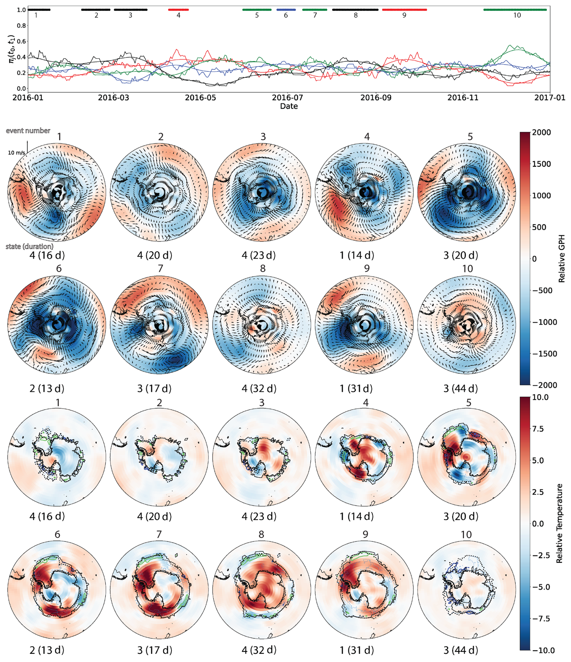
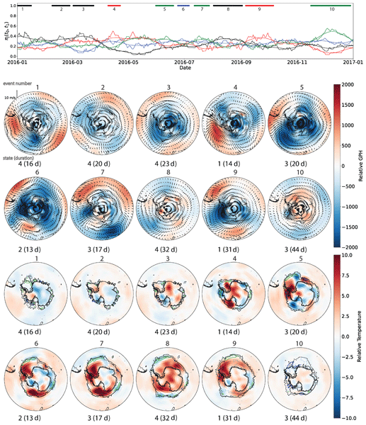
Figure 3 Persistent background events in 2016. Time series from the transition matrix with LOWESS overlay are shown; the states 1–4 are color-coded red, blue, green and black respectively including timings of the ten persistent background states (top panel). The lower panels show corresponding composite patterns of surface geopotential height anomalies (colored) and surface wind anomalies (arrows)(upper rows). The sea ice results (lower rows) depict surface temperature anomalies (colored), the SIE at the start of the event (dotted, black), the SIE at the end of the event (solid, black), and the sea ice concentration anomaly contours (dark blue = largest positive, green = largest negative). Each event is numbered and referenced in chronological order.

In general, the sequence of persistent events during 2016 are manifest in the major synoptic patterns. The PSA pattern in background event 6, coupled with the corresponding positive temperature anomalies over the Antarctic, appears to be the precursor that heralds the beginning of the major sea ice retreat observed in event 9. In event 9 we have a prominent metastable state 1, which differs significantly from previous metastable state 1 (event 4) in the atmosphere at lower latitudes. This change from event 4 to 9 highlights non-stationary changes to state 1. This change between events can also be observed when metastable state 3 is prominent, where the low patterns over Antarctica (events 5 and 7) change to the Antarctic warming pattern in event 10 (Franzke et al., 2015). The pattern correlations reveal the SAM and ASL patterns to be the prominent patterns throughout most of 2016, with the PSA2 (event 1, r=0.439), PSA1 (event 4, r=0.455), and Wave-4b (event 7, $r=-\mathrm{0.483}$) also contributing to the observed persistent states. Of note is the gradual increase in surface temperature anomalies around Antarctica throughout 2016 that starts in March and slowly builds until October. While the trapped heat around the Antarctic is a plausible explanation for the negative concentration anomalies toward the end of the year, anomalous warming alone cannot account for the rate and heterogeneity of the low ice events. Given the lag times between the occurrence of synoptic patterns and the regional changes in sea ice, we conclude that the low sea ice event in 2016 could be explained by the metastable characteristics of the synoptic flow. The prominent ASL and positive SAM present throughout event 9 transitions to a strong negative SAM in event 10. The recent study of Eabry et al. (2025) also notes the SAM transition from strongly positive in September to strongly negative in November which preceeds the SIE decline in 2016. Finally, while the signature of the SAM pattern can be observed intermittently throughout 2016 (e.g., pattern correlations >0.5 in events 2, 3, 5, 6, 9 and 10; also noted in Stuecker et al., 2017), its influence on the melt event depends on compounding factors and relative to other patterns such as PSA, ASL, or the Antarctic warming pattern.

3.2 2021–2022 case study

The results relating to 2021 are shown in Fig. 4, which illustrates eleven persistent background events distributed throughout the year. Of these, we have three state 1, two state 2, two state 3, and four state 4 events. This year begins with positive anomalies in sea ice concentration before dropping to more neutral levels towards the end of the year (Fig. 1). Anomalously high surface air temperatures in the vicinity of the Dronning Maud Land (event 2), the Weddell Sea (event 4) and, to a lesser extent the Ross Sea and George V Land (state 6), are associated with entrainment of warmer air via persistent onshore winds but not significantly correlated with any of the considered invariant climate patterns described in Table B2. Increasingly enhanced zonal winds characterize transition states (events 1, 3, 5) between the aforementioned warming patterns correlated with SAM (r>0.5) until a general warming pattern occurs over the entire Antarctic continent and sea ice zone in event 7 correlated with SAM (r>0.7). This warming pattern decays through events 8–11 from late October to January. However, from September onward, we observe a negative anomaly resembling the Amundsen Sea Low (ASL) that persists throughout the remaining events ($r\in [\mathrm{0.851},\mathrm{0.977}]$, with all amplitudes $min\left(Z_{\mathrm{1000}}^{\prime }\right)$ lower than −1481 hPa). The drop in sea ice concentration anomalies back to neutral levels (Fig. 1) coincides with events 9 through 11. In addition to the persistent ASL pattern present, a clear ZW3 structure can be seen in event 9 (r=0.527 for pattern ZW3A), a SAM pattern is observed in event 10 (as in many other patterns), and a zonal pattern in event 11. A uniform collapse in the sea ice occurs during event 9 onward, and this is accompanied by the gradual recapture of positive temperatures over the Antarctic.

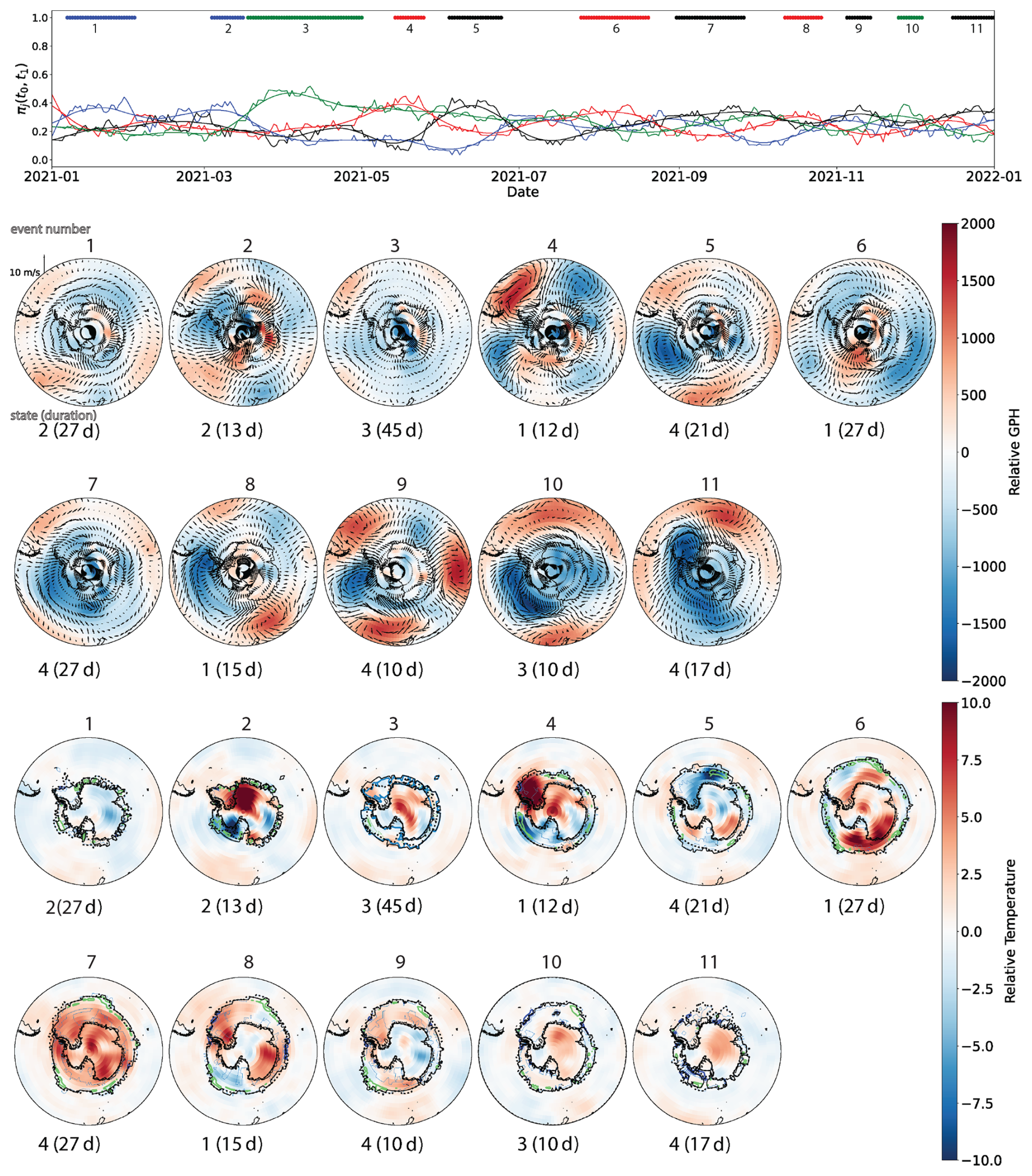
Figure 4 As for Fig. 3, but for the year 2021.

We note that the events for 2021 contrast markedly with those associated with 2016. Atmospheric background events transition through a sequence of zonal events; in particular, the zonal event 7 transitions through a composite wave-4 + ASL flow (event 8) and an ASL + ZW3 patterns with elements of SAM and PSA1 (event 9) to strongly zonal cases 10 and 11. This coincides with a zonally uniform contraction of SIE. The ASL patterns discussed in the literature (Turner et al., 2022; Wang et al., 2023) are reproduced in this model but are more shallow than the deep ASL events seen in other years (Table B4), such as event 9 in 2016 (Fig. 3). The anomalous surface warming in events 6 and 7 precedes the transition to a strongly zonal flow and a uniform rapid melting that occurs from the austral spring to the austral summer (events 9–11), and coincides with the decrease in sea ice concentration anomalies from positive to neutral at the end of 2021 (Fig. 1). Each event associated with a given metastable state differs from previous instances, where there are regional shifts in atmospheric patterns moving in space. Unlike 2016, however, we do not note any rapid changes in sign from one event to the next, with some metastable state events persistent throughout the year. For example, those events associated with metastable state 4 (events 5, 7, 9, 11) remain zonal patterns with mid-latitude highs or wavetrains throughout the year, and all have a common ASL pattern.

3.3 2023 case study

Finally, we summarize the events that occur during 2023 in Fig. 5 and Table B3. The nine events are divided into three state 1, two state 2, three state 3, and one state 4 event. Characterized by record low sea ice anomalies in the first half of the year (Fig. 1, Josey et al., 2024; Purich and Doddridge, 2023; Swathi et al., 2025), events 1–5 for the atmosphere start out as zonal patterns, but gradually shift towards wavetrain patterns by the midpoint. In particular, event 4 is a SAM-ASL pattern with the low-pressure system extending over the Bellinghausen Sea with the wind pushing into the Antarctic peninsula (r = 0.730 [SAM], 0.858 [ASL]). There is a noticeable absence of growth in sea ice until after event 4, especially around the Antarctic peninsula. The reduced growth, together with the general poleward wind vector anomalies, contributes toward the record low maximal SIE observed during 2023. Atmospheric patterns in the second half of the year (events 6 through 9) progress through a series of coherent structures, starting with wave-4b ($r=-\mathrm{0.699}$), then PSA2 ($r=-\mathrm{0.416}$), PSA1 (r=0.476), and finally SAM (r=0.674). As shown in event 8, a high-pressure anticyclonic system north of the Amundsen Sea extends over the Bellinghausen Sea into the Weddell Sea that is reminiscent of a PSA pattern, following a localized low pressure system over the Ross Sea. Finally, during event 9 a SAM pattern with weak zonal symmetry starts in October and extends into the new year. The synoptic patterns coincide with concentration anomalies that increase from a record negative to neutral by the end of the year (Fig. 1). They are accompanied by sustained trapped heat from events 2 to 8, which show significant positive temperature anomalies throughout the continent except for the Weddell Sea and the Ronne Ice Shelf. This heat-trapping manifests during event 9 as an uneven melt during which sea ice in the Weddell Sea remains stable, while collapsing in an almost uniform manner elsewhere.

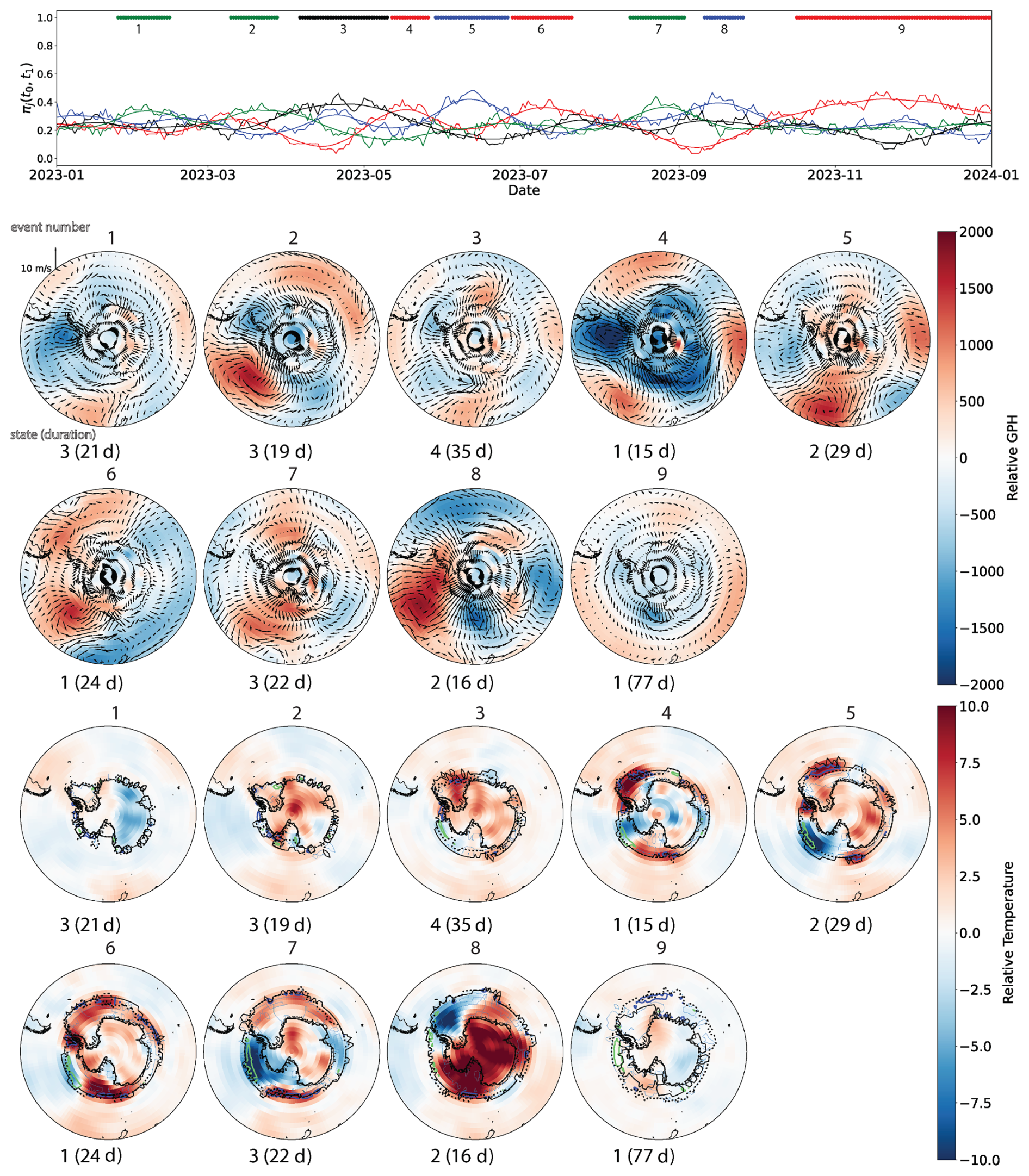
Figure 5 As for Fig. 3, but for the year 2023.

On the basis of pattern correlations, we conclude that the 2023 background events are comprised of more synoptic wave patterns than zonal flows; in this regard it is similar to 2016. In particular, we notice synoptic patterns in events 4 (SAM + ASL) and 8 (PSA1) that influence how sea ice forms and melts throughout the year. The record low maximum extent, in particular, is influenced by the sea ice formation in the Antarctic peninsula, which takes until September to fully develop. This is in line with the study of Josey et al. (2024), who also note that these areas around the peninsula (particularly the Ross, Bellinghausen, and Weddell seas) exhibit up to an 80 % reduction in sea ice concentration during the austral autumn of 2023. The return to neutral levels of sea ice by the end of the year is a result of event 8. Synoptically, we have a PSA1 pattern with a high extending to the Weddell Sea, but in terms of the surface temperatures, we find that the Antarctic is significantly warmer than usual (up to 10 °C) with colder temperatures over the Weddell Sea. This pattern plays a significant part in the melt season over the course of event 9. During this time, while the sea ice melts rapidly elsewhere, the sea ice over the Weddell Sea melts far more slowly, leading to significantly more sea ice in that region. This high concentration in the region helps contribute to the sea ice anomalies which return to neutral levels at the end of the year (Fig. 1). Events that are associated with a common metastable state tend to display reduced diversity and increased structural similarities. This is reminiscent of the behavior in 2021, except we find regional sign changes in 2023. For example, events associated with metastable state 1 (events 4, 6, 9) and metastable state 2 (events 5, 8) witness a change in sign in the south-west Pacific from lows in their first event to highs in later events.

4 Discussion

Our analysis of the persistent atmospheric patterns around the major low sea ice events over recent years highlights that the three cases share some common properties, while also exhibiting significant differences. We observe that these recent record low events are preceded by anomalous surface warming over the Antarctic, as one might expect. However, persistent synoptic features in the atmosphere are also crucial for the occurrence of anomalous events, with the nature of these driving the observed heterogeneity. In short, the 2016 and 2023 anomalous low ice events are strongly influenced by synoptic patterns, leading to highly asymmetric events by the end of the year. Melting in the Amundsen Sea (2016) is accelerated by an ASL pattern, while the melting in the Weddell Sea (2023) is slowed by a combination of high air pressure and low air temperature anomalies (see Figs. 3 and 5). By way of contrast, the 2021 anomalous low ice event is much more uniform as a consequence of zonal patterns (Fig. 4).

We have seen examples of sea ice asymmetry during 2023, characterized by a slow growth around the Antarctic Peninsula and subsequent slow melt rates in the Weddell Sea (Fig. 5). The corresponding patterns in the atmosphere are also asymmetric. This confirms the findings of Schroeter et al. (2023), who identified decreasing zonal symmetry with respect to SAM in recent years. This breakdown of zonal symmetry in SAM patterns can be observed in cases such as event 10 of 2021 (Fig. 4) or event 9 of 2023 (Fig. 5). Here SAM patterns can be detected, but there is a reduction in zonal symmetry throughout the respective events relative to the canonical annular SAM state. This could also provide a possible explanation for why we find that SAM is seen to act most frequently in unison with the ASL, and less frequently the PSA, in terms of correlations to the atmospheric modes of variability during the years considered. Although some studies have predicted a negative SAM index during the 2016 austral spring and propose it as a possible driver for the 2016–2017 sea ice melt season (Schlosser et al., 2018), our findings suggest that this result could be purely coincidental when other atmospheric mechanisms are taken into account.

Our analysis based on multivariate optimization has attempted to analyze the relative roles of thermodynamic versus dynamical process in relation to characteristics specific to the atmospheric modes of variability that covary with sea ice concentration and extent. For instance, SAM acts on sea ice as a largely dynamical process regulating the westerly winds at lower latitudes whose low frequency variability is further modulated by the phase i.e., the positive SAM phase shifts the westerlies towards Antarctica, compacting sea ice towards the continent, while the negative phase shifts westerlies away from Antarctica with a dispersal effect on sea ice. It has been conjectured that SAM phases during the austral summer can impact sea ice development with positive phases having cooler Antarctic temperatures and negative with warmer (Boehm et al., 2025; Chan et al., 2025; Doddridge and Marshall, 2017) however, from the analysis described above, we see less evidence for this during the record low sea ice events considered here. In contrast to the zonal SAM, the PSA and ASL synoptic patterns both primarily impact the Amundsen-Bellinghausen Sea's and their immediate neighboring regions. The ASL in particular strengthens offshore winds in the sector while pushing sea ice northward from the Ross sea and transporting warmer air towards the Antarctic Peninsula, negatively affecting sea ice development in the Bellinghausen sector (Holland et al., 2018; Wang et al., 2023). Meanwhile, the PSA patterns act as a bridge between tropical modes such as the El-Niño southern oscillation and Antarctic modes in the western hemisphere (Gurjão et al., 2025). Finally, the ZW3 pattern, being a tripolar wavetrain, impacts the Antarctic depending on the advection of warm (ocean) or cold (land) surface air temperatures due to cyclonic and anticyclonic flow relative to the positioning of the respective highs and lows in geopotential height corresponding to ZW3. This usually comes in the form of transporting warm air southward (pushing back and melting sea ice) while expanding sea ice in areas with northward winds, with the effects mostly felt in the Amundsen-Bellinghausen sectors (Eabry et al., 2024; Schlosser et al., 2018).

The results of this study help highlight the difference between a local, non-stationary analysis and a global, stationary analysis. Many previous studies using stationary analyses (e.g. Schlosser et al., 2018; Stuecker et al., 2017) capture fixed-timescale dynamics in a way that detects patterns that operate on the chosen timescale, but are less successful in identifying any structures that evolve on either longer or shorter timescales. This can give rise to somewhat misleading results: shorter timescale patterns (e.g., the ZW3 pattern in event 9 of 2021, Fig. 4) tend to be filtered out or reduced in strength. On the other hand, longer timescale patterns such as the Antarctic warming pattern of Franzke et al. (2015), seen in event 10 of Fig. 3, are often not fully developed owing to the pattern duration being cut off prematurely by the prescribed temporal boundaries. Here, we have shown how a non-stationary analysis, in which the event temporal boundaries are defined by the model itself, can be used to capture all of these atmospheric patterns across varying timescales. This is particularly useful in problems that involve interacting systems with a range of timescales such as atmospheric synoptic patterns and sea ice, providing a framework for future development of non-stationary analyses.

Our results suggest some possible future directions for study. First, we have only considered the case where the 200, 500, and 850 hPa geopotential height datasets are coupled with sea ice concentration for generating the FEM-BV-VAR model. A possible extension to this study could be to analyze models optimized for a single season or sector. Such an analysis should highlight changes in more localized instances in space or time, such as the Amundsen Sea region for sectors, or more seasonal factors. The use of multivariate stacking with sea ice concentration and geopotential height could be used as a springboard for different couplings, such as sea ice and ocean temperatures for ocean-based drivers, or a full atmosphere-ocean-ice coupling in the FEM-BV framework to observe how covariations in the chosen variables influence the identification of metastable processes in ice formation and retreat. Such a study should enable the development of a more complete picture of important processes looked at from a non-stationary perspective. A more extensive and comprehensive study could consider the method applied to different reanalysis products. Datasets such as ERA5 and JRA55 could be utilized in a similar manner to the NNR1 reanalysis used here, and the resulting model behavior would enable improved understanding of how the choice of dataset and reanalysis bias influences the results obtained.

In summary, we have embedded a multivariate dataset based on sea ice concentration and geopotential height within a reduced-order model. We have extracted the persistent background events using transition matrix methods on years associated with record lows in sea ice around Antarctica, and have interpreted these to derive a clearer picture of how sea ice covaries with changes in the atmosphere. The results of this study illustrate how a non-stationary approach can be applied for the analysis of coupled systems that act over a range of timescales. This sheds light on the underlying processes of anomalous low ice events.

Appendix A: Finite Element Bounded Variation Vector Auto-Regressive optimisation: FEM-BV-VAR

We provide an outline of the FEM-BV-VAR process used to derive the requisite affiliation sequences. Variable and other definitions are provided in Table A1.

Table A1 A glossary of terms and variables used in the FEM-BV-VAR process. The left column describes the main equations and key variables used in the algorithm, with the variables and terms defined in the right column. These are ordered in a linear fashion such that those further down are performed later in the algorithm.

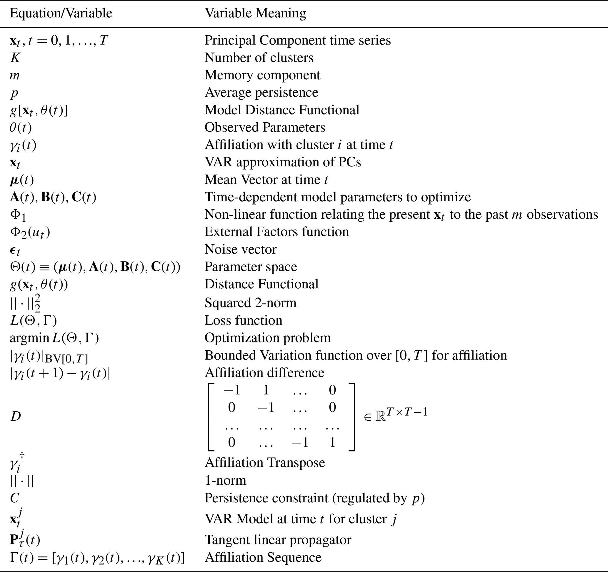
We start by inputting training data in terms of principal components x_t and chosen hyperparameters for number of clusters K, memory component m, and average persistence p. We then define a model distance functional

$$\begin{array}{}\text{(A1)}& g[{\mathbf{x}}_t,\mathit{\theta }(t\left)\right]=\sum _{i=\mathrm{1}}^K{\mathit{\gamma }}_i\left(t\right)g({\mathbf{x}}_t,{\mathit{\theta }}_i(t\left)\right))\end{array}$$

as a linear combination of affiliations and distance functionals, where the affiliations are subject to convexity constraints (each affiliation γ_i(t) is non-negative, and the sum of affiliations at every given point in time must equal 1). The distance functionals are defined as the square of the approximation error between the principal component and its vector-autoregressive (VAR) approximation in Euclidean space (with stochastic factors omitted). The VAR approximation itself is the sum of its mean vector, the memory component relating present day and its past approximations, the external factors, and stochastic noise. It is given by

$$\begin{array}{}\text{(A2)}& \begin{array}{rl}{\mathbf{x}}_t& \approx \mathit{\mu }\left(t\right)+\mathbf{A}\left(t\right){\mathrm{\Phi }}_{\mathrm{1}}({\mathbf{x}}_{t-\mathit{\tau }},{\mathbf{x}}_{t-\mathrm{2}\mathit{\tau }},\mathrm{\dots },{\mathbf{x}}_{t-m\mathit{\tau }})\\ & +\mathbf{B}\left(t\right){\mathrm{\Phi }}_{\mathrm{2}}\left(u_t\right)+\mathbf{C}\left(t\right){\mathit{ϵ}}_t.\end{array}\end{array}$$

In addition to the stochastic factors being omitted, we also do not consider external factors for our study so we assume that $\mathbf{B}\left(t\right)=\mathbf{0}\forall t$. As such, the distance functional becomes

$$\begin{array}{}\text{(A3)}& g({\mathbf{x}}_t,\mathit{\theta }(t\left)\right)=\left|\right|{\mathbf{x}}_t-\mathit{\mu }\left(t\right)-\mathbf{A}\left(t\right){\mathrm{\Phi }}_{\mathrm{1}}({\mathbf{x}}_{t-\mathit{\tau }},\mathrm{\dots },{\mathbf{x}}_{t-m\mathit{\tau }})|{|}_{\mathrm{2}}^{\mathrm{2}}.\end{array}$$

With the model distance functional defined and fixed hyperparameters chosen, we minimize the loss function L(Θ,Γ) to determine the optimal VAR model parameters and affiliations via simulated annealing and with an additional temporal regularization constraint

$$\begin{array}{}\text{(A4)}& L(\mathrm{\Theta },\mathrm{\Gamma })=\sum _{t=\mathrm{0}}^T\sum _{i=\mathrm{1}}^K{\mathit{\gamma }}_i\left(t\right)g({\mathbf{x}}_t,{\mathit{\theta }}_i(t\left)\right)\to \text{argmin }L(\mathrm{\Theta },\mathrm{\Gamma }).\end{array}$$

The bounded variation or temporal regularisation, is constrained by C which governs the maximum allowed number of transitions between clusters over all data instances in the interval [0,T], achieved through the 1-norm, transposition of affiliations, and matrix D. This is defined through

$$\begin{array}{}\text{(A5)}& \left|{\mathit{\gamma }}_i\right(t){|}_{\mathrm{BV}[\mathrm{0},T]}=\sum _{t_{\mathrm{0}}}^{T-\mathrm{1}}|{\mathit{\gamma }}_i(t+\mathrm{1})-{\mathit{\gamma }}_i\left(t\right)|=|\left|\mathbf{D}{\mathit{\gamma }}_i^{†}\right|{|}_{\mathrm{1}}\le C.\end{array}$$

Once the optimal time dependent model parameters Θ have been determined, we obtain the VAR model

$$\begin{array}{}\text{(A6)}& {\mathbf{x}}_t^j:={\mathit{\mu }}^j\left(t\right)+\sum _{\mathit{\tau }=\mathrm{1}}^m{\mathbf{P}}_{\mathit{\tau }}^j\left(t\right){\mathbf{x}}_{t-\mathit{\tau }}+{\mathit{ϵ}}_t,\end{array}$$

and the affiliation sequence

$$\begin{array}{}\text{(A7)}& \mathrm{\Gamma }\left(t\right)=\left[{\mathit{\gamma }}_{\mathrm{1}}\right(t),{\mathit{\gamma }}_{\mathrm{2}}(t),\mathrm{\dots },{\mathit{\gamma }}_K(t\left)\right].\end{array}$$

In this study, we only require the affiliation sequence to achieve our results. We refer the interested reader to the works of Horenko (2010) and Metzner et al. (2012) for the methodology and to Axelsen et al. (2025) for further information and some examples of application to persistent states of the Southern Hemisphere troposphere.

Cross validation

In order to classify models we use the following cross-validation procedure following Quinn et al. (2021). First, for a given choice of hyperparameters K, m, and p, the data is divided into N_fold+1 equal length segments 𝒯₁, …, ${\mathcal{T}}_{N_{\mathrm{fold}}+\mathrm{1}}$, and each model refit N_fold times, where on the ith iteration the first i segments are used as the training sample. Holding the obtained state parameters $\widehat{\mathrm{\Theta }}$ fixed, affiliations are calculated by minimizing the cost function (Eq. A4) evaluated over the (i+1)th segment, adjusting the upper bound set by the peristency constraint C as appropriate for the length of the segment with fixed p. The weighted root-mean-square error

$$\begin{array}{}\text{(A8)}& {\mathrm{RMSE}}_i=\sqrt{{\displaystyle \frac{\mathrm{1}}{d({\mathcal{T}}_i-m_{max})}}\sum _{t\in {\mathcal{T}}_{i+\mathrm{1}}}\sum _{j=\mathrm{1}}^K\left[{\mathit{\gamma }}_t{]}_j\right||{\mathbf{x}}_t-{\widehat{{\mathbf{x}}_t}}^{\left(j\right)}|{|}^{\mathrm{2}}}\end{array}$$

is then evaluated for each test segment. Here d is the number of PCs retained, and ${\widehat{\mathbf{x}}}_t^{\left(j\right)}$ denotes the expected value under cluster j, which is determined from the training data.

This cross-validation process yields a distribution for each model in terms of the mean RMSE and a standard error, which accounts for the uncertainty in predicting the true RMSE of a model. In lieu of estimates of out-of-sample prediction error, we use the mean reconstruction RMSE over the set of test sets as a measure of the ability of the model to generalize to future data. This requires evaluating model performance as a compromise between model flexibility and overfitting the training data. Estimation of the out-of-sample forecast error, would require an additional model for the dynamics of the hidden switching process which the Markov transition potentially provides but which we here leave to future work.

Appendix B: Canonical atmospheric modes and confidence

Here we provide a table of pattern correlations between each background event covered in Figs. 3, 4, and 5 and known invariant patterns (in addition to anomaly amplitudes in the Amundsen Sea region). We compare with the following:

• –

  the leading five EOFs of the Southern Hemisphere as described in Axelsen et al. (2025):

  • –

    Southern Annular Mode (SAM),

  • –

    Pacific-South American teleconnection PSA1,

  • –

    Pacific-South American teleconnection PSA2,

  • –

    Wave-train pattern Wave-4a, and

  • –

    Wave-train pattern Wave-4b,

• –

  the Amundsen Sea Low (ASL) – The leading geopotential height EOF calculated in the region covered by 60–80° S, 170–298° E) (Hosking, 2025),

• –

  Higher order hemispheric EOF for meridional v-winds, Zonal Wave 3 A (ZW3A), and

• –

  Higher order hemispheric EOF for meridional v-winds, Zonal Wave 3 B (ZW3B),

  • –

    where the ZW3 patterns are described in Goyal et al. (2022).

Each EOF is calculated for the full time period and the correlations are given in Tables B1 (2016), B2 (2021), and B3 (2023). For two given sets of data B_i and C_i, with i ∈ $\mathit{\{}\mathrm{1},\mathrm{\dots },V\mathit{\}}$, we define the pattern correlation coefficient r(B,C) for the two patterns by

$$\begin{array}{}\text{(B1)}& r(B,C):={\displaystyle \frac{{\sum }_{i=\mathrm{1}}^V{B}_i{C}_i}{\sqrt{{\sum }_{i=\mathrm{1}}^V(B_i{)}^{\mathrm{2}}}\sqrt{{\sum }_{i=\mathrm{1}}^V(C_i{)}^{\mathrm{2}}}}}.\end{array}$$

We remark that while the pattern correlations are a very important part of establishing confidence in synoptic features for a given event, the amplitudes of the anomalies is just as crucial. For example, knowledge of both the amplitude of the anomaly in the ASL and the pattern correlations is required to establish the presence of a deep ASL event. Event 3 of 2021 (Fig. 4) is very strongly positively correlated with the ASL (r=0.941, Table B2), but the low itself is significantly shallower relative to most other strong positive correlations ($min\left(Z_{\mathrm{1000}}^{\prime }\right)\approx -\mathrm{752}$, compared to upwards of −2566 in event 5 of 2016). We provide a table of lowest surface pressure anomalies $min\left(Z_{\mathrm{1000}}^{\prime }\right)$ for all significantly positively correlated events with ASL in Table B4.

Table B1 Pattern correlations for each event occurring in 2016 (Fig. 3) compared to each of the atmospheric modes mentioned in this appendix. We bold all correlation coefficients with a magnitude greater than 0.4 to highlight those of sufficient significance that we can be confident that the pattern is embedded in the event. In the cases where we have a significant positive correlation with ASL, we refer to Table B4 for the amplitude of the surface pressure anomaly to confirm confidence in the particular atmospheric mode.

Table B2 As Table B1, but for 2021 (for the events in Fig. 4).

Table B3 As Table B1, but for 2023 (for the events in Fig. 5).

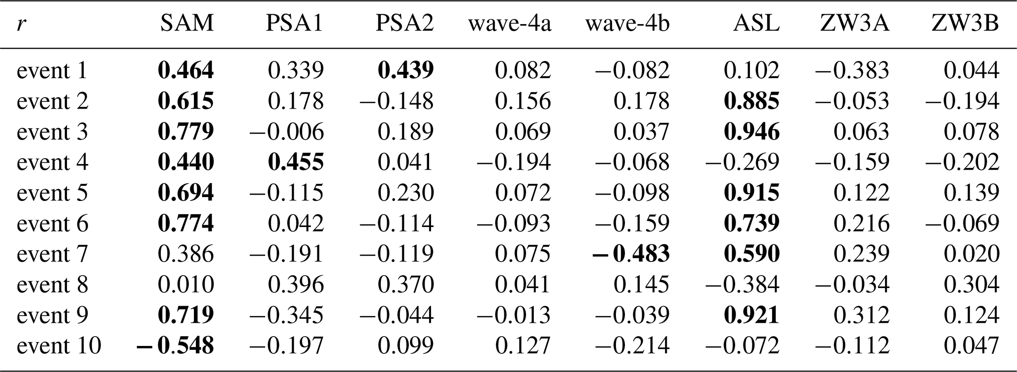
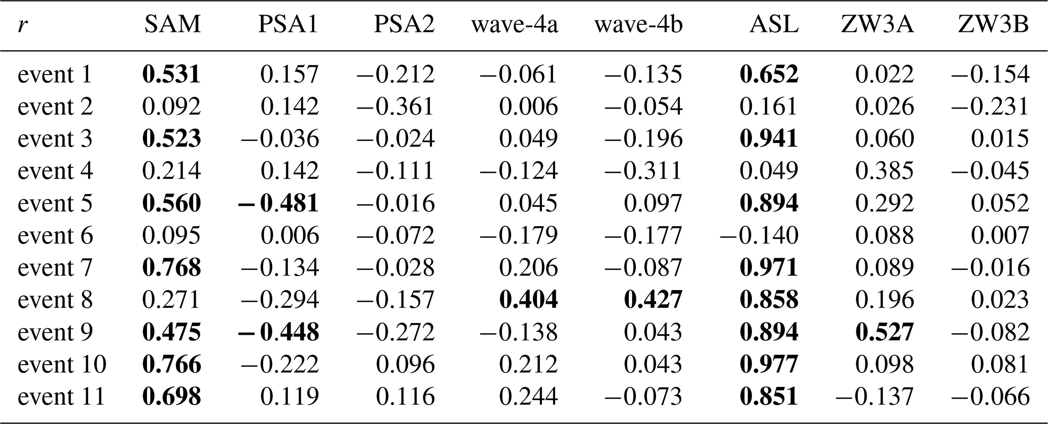
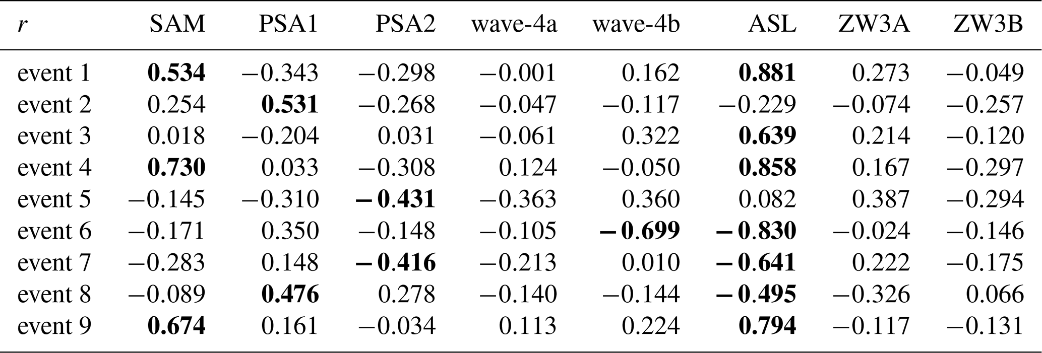
Table B4 Events that have a significant positive correlation with ASL in Tables B1, B2, and B3. We have calculated the lowest surface pressure anomaly $min\left(Z_{\mathrm{1000}}^{\prime }\right)$ over the composited event over the Amundsen Sea region using the boundaries described by Hosking (2025). Shown in bold is the event with the deepest regional surface pressure anomaly for each year, and dashes indicate events that either have no significant correlation, are negatively correlated with ASL, or do not exist. All values are rounded to the nearest integer. This table, in conjunction with the pattern correlation Tables B1–B3, gives us a way to gauge the level of confidence in deep ASL events, as well as validation for the claim made with respect to the depths of ASL events in 2021.