Beyond static forecasts: a dynamic stress gradient framework for high-resolution aftershock prediction and mitigation

Accurate forecasting of aftershock distributions is vital for effective post-earthquake emergency response, early warning systems, and long-term seismic hazard mitigation. This study introduces a novel nonlinear, multiscale framework for modeling the evolution of Coulomb stress following a major earthquake. The proposed approach integrates rate-and-state friction laws, a KPP-type reaction–diffusion equation, and the Banach fixed-point theorem to simulate the dynamic redistribution of stress in space and time. Central to the model are two time-dependent parameters – α(t), which governs the decay of stress memory consistent with Omori's law, and β(t), which modulates the nonlinear diffusion and reaction dynamics. Applied to the 2018 Hualien earthquake in Taiwan, the framework resolves stress changes and their gradients at depths of 6–25 km. Results indicate that stress gradients are more predictive of aftershock occurrences within the first 50 d and at depths shallower than 12 km, while stress changes play a dominant role at greater depths and later times. Validation using AUC and Molchan error metrics demonstrates the model's strong spatial forecasting capability. The framework's adaptive convergence and modular structure support real-time seismic hazard assessment and integration into PSHA workflows, offering a promising tool for aftershock modeling and disaster resilience planning.

1 Introduction

Developing a precise stress evolution model that can rapidly predict the timing and location of aftershocks following a massive earthquake is of immense value. Such a model would enhance disaster preparedness, optimize resource allocation, and mitigate the devastating effects of aftershocks, ultimately safeguarding lives and reducing the risk of further losses caused by aftershock damage. The occurrence of aftershocks is intricately tied to stress changes induced by the mainshock, and the evolution of post-seismic stress over time plays a pivotal role in predicting aftershocks (Devries et al., 2018; Aden-Antoniow et al., 2022). Located at the active collision boundary between the Eurasian and Philippine Sea plates, Taiwan is characterized by rapid convergence and high seismicity. Early studies (Tsai et al., 1977; Wu, 1978) demonstrated that the spatial distribution of earthquakes across the island reflects complex interactions among subduction, arc–continent collision, and inherited crustal structures. Rather than being random, seismicity is primarily controlled by regional tectonic regimes and evolving stress fields. Such tectonic complexity promotes heterogeneous stress transfer, making Taiwan a premier natural laboratory for studying postseismic stress evolution and aftershock triggering processes.

Furthermore, seismic stress evolution is fundamental to advancing our understanding of earthquake mechanics and the associated risks. The complex interplay of processes governing stress accumulation and release in the Earth's crust underscores the need for more comprehensive modeling approaches. A modeling framework that can simulate post-seismic stress redistribution and identify potential earthquake-triggering zones is essential for improving seismic risk assessment and management. However, despite much progress, a comprehensive theory explaining how post-earthquake stress evolves and leads to aftershocks remains elusive.

In the evaluation of aftershock locations, the primary focus is on the application of Coulomb stress change. The Coulomb stress model has been a foundational tool for understanding fault interactions and stress transfer during seismic events (King et al., 1994). By quantifying shear and normal stress changes, it evaluates aftershock potential and fault stability under diverse tectonic conditions (Harris, 1998). Early foundational work by Mignan and King (2007) formulated accelerating moment release based on stress accumulation and transfer models, establishing a framework for exploring stress interactions. Subsequent studies expanded the application of the Coulomb model to various geological contexts, such as stress evolution in subduction zones (Hsu et al., 2006) and fault systems like the Dead Sea Fault (Heidbach and Ben-Avraham, 2007) and Tien Shan (Pang, 2022). Specific earthquake events further illustrate the model's utility. For example, research on the 1999 Chi-Chi earthquake in Taiwan revealed how stress redistribution influences afterslip, relaxation, and deviations from Omori decay (Chan and Stein, 2009). Analyses of the 2008 Wenchuan earthquake demonstrated cascading stress effects on subsequent seismic events (Zhang et al., 2013), while viscoelastic relaxation studies enhanced understanding of stress redistribution in Sichuan (Xie et al., 2022). Similarly, Coulomb stress models of earthquake sequences have underscored how historical stress changes can influence fault behavior and trigger seismic activity, respectively (Nathan and Walter, 2020; Tang et al., 2023; Ueda and Kato, 2023). Long-term investigations, such as those on the East Kunlun Fault Zone (Shan et al., 2015) and the Sulaiman Lobe (Ali et al., 2017), highlighted the model's potential for assessing regional seismic hazards. While the Coulomb stress model has significantly advanced our understanding of stress transfer and fault interactions, its typical applications often focus on isolated events or discrete timeframes. This limitation restricts its ability to capture the continuous evolution of stress fields, which is essential for modeling dynamic aftershock sequences and improving seismic hazard assessments.

Secondly, combining the Rate-and-State (R-S) physical model to explore stress transfer near faults and understand the mechanisms of aftershock generation represents an advanced development. The R-S friction model, first introduced by Dieterich (1994), has been instrumental in describing the relationship between stress and friction on faults. Grounded in Coulomb stress and friction constitutive laws, the model provides a robust framework for investigating earthquake nucleation and fault mechanics. Early work by Ampuero and Rubin (2008) explored aging and slip laws within the R-S framework, offering critical insights into the processes governing earthquake initiation. Building on this foundation, Barbot et al. (2012) advanced the model by integrating short-term earthquake dynamics with long-term geological processes, enhancing its capacity to simulate seismic cycles and their broader implications. Recent applications highlight the model's adaptability to diverse tectonic settings. Javed et al. (2016) integrated Coulomb failure and R-S models to replicate the Omori-Utsu relation for aftershock decay, shedding light on stress shadowing effects and the temporal evolution of seismicity. Pranger et al. (2022) further expanded the model by combining R-S friction with transient viscous flow principles, resulting in a more comprehensive representation of fault dynamics. Su et al. (2024) applied R-S friction principles to estimate earthquake probabilities along the Liupanshan Fault, demonstrating its potential for probabilistic seismic hazard assessments. Despite these advances, the R-S model faces inherent challenges in addressing the spatiotemporal complexities of stress evolution. High friction parameters can lead to numerical divergence, limiting the model's applicability in heterogeneous tectonic settings. Furthermore, localized implementations, while computationally efficient, often lack mechanisms for stress diffusion, restricting their ability to capture interactions across larger fault systems. Overcoming these limitations requires the integration of additional diffusion processes and stability mechanisms to better address the interplay between localized and distributed stress evolution. Such advancements are essential for improving the model's predictive power and its applicability in seismic hazard assessments.

Finally, the distribution of aftershocks provides other valuable insights into seismic stress dynamics, with the widely recognized Omori Law describing the temporal decay of aftershock sequences (Utsu, 1961). While empirical laws offer foundational understanding, theoretical models have advanced this knowledge by incorporating reaction-diffusion frameworks, such as the Kolmogorov-Petrovsky-Piskunov (KPP) equation, to capture complex postseismic behaviors. Building on this transition from empirical to mechanistic modeling, we employ a KPP-type reaction–diffusion framework to characterize the dynamics of stress redistribution, as formulated by Kolmogorov et al. (1991) and El-Hachem et al. (2019). Guglielmi et al. (2021) demonstrated the utility of the KPP equation for understanding stress propagation in seismic contexts. Regenauer-Lieb et al. (2021) further highlighted its application through cross-diffusion-driven wave processes, transforming the KPP framework into a dynamic wave-driven stress diffusion model that aligns its diffusion-reaction characteristics with the evolving stress field more effectively. Recent studies have reinforced the promise of the KPP framework for capturing aftershock evolution. For instance, Zavyalov et al. (2022) applied the KPP equation to model the spatial and temporal dynamics of aftershock distributions following mainshock events. Complementing these approaches, nonlinear equations such as the Fisher equation have been employed to model wave propagation and spatial diffusion in geological settings, further enhancing understanding of stress distribution (Alqahtani et al., 2024).

However, despite its effectiveness in modeling stress diffusion, the KPP equation has notable limitations. It does not directly incorporate frictional behavior and is prone to numerical instability in heterogeneous tectonic environments, which restricts its broader applicability. To overcome these challenges, Banach's Fixed-Point Theorem (Granas and Dugundji, 2003) offers a robust mathematical framework for ensuring numerical stability. By conceptualizing the stress release process as an iterative contraction mapping, the theorem guarantees convergence to a stable state after a destructive earthquake. The integration of Banach's Fixed-Point Theorem with the KPP model marks a significant advancement over conventional stress modeling approaches. By resolving issues of numerical divergence and improving stability in nonlinear stress propagation scenarios, this combined framework provides a more comprehensive and reliable method for capturing the intricate dynamics of aftershock sequences and stress evolution.

Building on this foundation, this study introduces a novel integration of the Rate-and-State (R-S) friction model, the KPP equation, and Banach's Fixed-Point Theorem. The KPP equation effectively models spatial stress diffusion, the R-S friction model captures nonlinear stress accumulation and slip behaviors along rocks, and Banach's theorem ensures numerical convergence by addressing challenges in heterogeneous tectonic environments. This integrated framework overcomes critical challenges in simulating stress redistribution across depths and time scales, offering a robust approach for aftershock forecasting. This comprehensive framework not only advances the understanding of fault mechanics and stress evolution but also bridges theoretical advancements with practical applications in seismic hazard mitigation. By effectively modeling post-earthquake stress evolution and aftershock distributions, this approach facilitates the precise identification of high-risk areas and temporal patterns of seismic activity. Such insights enable the strategic deployment of emergency response teams, the optimized allocation of relief resources, and the prioritization of inspections and reinforcements for vulnerable infrastructure.

Moreover, incorporating this model into disaster preparedness frameworks enhances risk communication and raises community awareness, empowering residents to take proactive measures to safeguard their lives and properties. Over the long term, this methodology can guide the design and retrofitting of seismic-resistant infrastructure, strengthening communities' ability to withstand future earthquakes. By translating predictive insights into actionable strategies, this research bridges the gap between theoretical advancements and practical disaster resilience, promoting safer, more sustainable urban environments.

2 Methodology

2.1 The iterative process of Coulomb's stress changes

This study integrates diffusion and reaction dynamics into a unified stress evolution framework. The methodology ensures numerical stability and convergence, enabling robust simulations of stress redistribution after earthquakes. When deriving a seismic source slip model, the initial spatial distribution of Coulomb stress changes, $\mathit{\sigma }\left(\mathit{x},t=\mathrm{0}\right)=\mathit{\sigma }\left(\right(x_{\mathrm{1}},x_{\mathrm{2}}),t=\mathrm{0})$, $\mathit{x}=(x_{\mathrm{1}},x_{\mathrm{2}})\in \mathrm{\Omega }\subset R^{\mathrm{2}}$, is calculated using the Okada method (1985) for specified depths and initial conditions:

$$\begin{array}{}\text{(1)}& \mathrm{\Delta }\mathrm{CFF}=\mathit{\sigma }\left(\mathit{x},t=\mathrm{0}\right)=\mathrm{\Delta }\mathit{\tau }+{\mathit{\mu }}^{\prime }\left(\mathrm{\Delta }{\mathit{\sigma }}_{\mathrm{normal}}\right)\end{array}$$

where Δτ is the shear stress change, μ^′ is the effective friction coefficient which is generally set to 0.4 (King et al., 1994), Δσ_normal is the normal stress change. In this research, the coseismic slip model used in the Coulomb stress change calculation was derived from Liao et al. (2024), which employed GPS data and GA inversion methods. The corresponding aftershock catalog was obtained from the Central Weather Administration (CWA) of Taiwan, with hypocentral locations refined using double-difference relocation, and is publicly accessible at https://www.cwa.gov.tw/V8/E/E/index.html (last access: 10 March 2026). The present model focuses on the temporal evolution of coseismic stress perturbations rather than on the absolute stress state of the lithosphere. Accordingly, the total stress field is conceptually decomposed as

$$\begin{array}{}\text{(2)}& {\mathit{\sigma }}_{\mathrm{total}}(\mathit{x},t)={\mathit{\sigma }}_{\mathrm{bg}}\left(\mathit{x}\right)+\mathit{\sigma }(\mathit{x},t)\end{array}$$

where σ_bg(x) represents the time-invariant background stress associated with long-term tectonic loading, topography, and bathymetry – while σ(x,t) denotes the earthquake-induced stress perturbation. Within this formulation, vertical loading effects are not neglected but treated implicitly. Differences in lithostatic loading between onshore and offshore regions, as well as variations associated with crustal structure, are incorporated into the rupture process and therefore embedded in the initial stress perturbation σ(x,0), which is derived from elastic dislocation modeling constrained by geodetic and seismological observations. The subsequent postseismic evolution is governed solely by the redistribution of σ, ensuring a physically consistent and mathematically well-posed description of stress relaxation. This formulation follows a perturbation-based stress evolution framework, where only the coseismic stress perturbation is dynamically evolved, while background lithostatic and tectonic loading set the equilibrium reference state.

To model post-earthquake stress evolution, we adopt a reaction–diffusion framework inspired by the Kolmogorov–Petrovsky–Piskunov (KPP) equation (Zavyalov et al., 2022), which captures the interplay between stress propagation and local reaction processes:

$$\begin{array}{}\text{(3)}& \partial \mathit{\sigma }(\mathit{x},t)/\partial t=D\left(z\right){\mathrm{\nabla }}^{\mathrm{2}}\mathit{\sigma }\left(\mathit{x}\mathbf{,}\mathit{t}\right)+f\left(\mathit{\sigma }(\mathit{x},t),\mathit{\theta }(\mathit{x},t)\right)\end{array}$$

where $D\left(z\right)=D_x=D_y$ represents the diffusion coefficient and varies only with depth z but is spatially uniform within each horizontal layer, reflecting the lack of reliable constraints on lateral anisotropy at regional scale and following standard practice in postseismic stress-diffusion modeling. The term ∇²σ(x,t) denotes the Laplacian of the stress field, which describes stress propagation. The stress reaction term $f\left(\mathit{\sigma }\right(\mathit{x},t),\mathit{\theta }(\mathit{x},t\left)\right)$ is a nonlinear reaction term that reflect Rate-and-State (R-S) friction behavior as well as stress saturation at high-stress levels, accounting for both stress buildup and frictional weakening. To reflect the influence of fault healing and time-dependent frictional behavior, the reaction term includes a logarithmic dependence on the state variable θ(x,t), inspired by Dieterich (1994) and Ampuero and Rubin (2008). It is presented as

$$\begin{array}{}\text{(4)}& \begin{array}{rl}& f\left(\mathit{\sigma }(\mathit{x},t),\mathit{\theta }(\mathit{x},t)\right)=A\left(z\right)\mathit{\sigma }(\mathit{x},t)\left(\mathrm{1}-{\displaystyle \frac{\mathit{\sigma }\left(\mathit{x}\mathbf{,}\mathit{t}\right)}{{\mathit{\sigma }}_{max}}}\right)\\ & +B\left(z\right)\log \left({\displaystyle \frac{\mathit{\theta }(\mathit{x},t)}{{\mathit{\theta }}_{\mathrm{0}}}}\right)\end{array}\end{array}$$

The first term models stress accumulation and saturation, ensuring the reaction vanishes at both zero and maximum stress ($\mathit{\sigma }(\mathit{x},t)=\mathrm{0}$ and $\mathit{\sigma }(\mathit{x},t)={\mathit{\sigma }}_{max}$), analogous to logistic growth. The second term captures the aging effect which means the longer the contact time (higher θ), the stronger the frictional resistance. Parameters A and B govern the magnitude of these effects and are allowed to vary with depth are described as

$$\begin{array}{}\text{(5)}& {\displaystyle }A\left(z\right)=A\mathrm{0}\exp (-z/L_a)\text{(6)}& {\displaystyle }B\left(z\right)=B\mathrm{0}\exp (-z/L_b)\end{array}$$

where z represents depth and $Ax=Ay=A\left(z\right)$, and $Bx=By=B\left(z\right)$ are assumed to be horizontally isotropic within each depth slice, L_a and L_b are characteristic depths that influence the variation of friction parameters with depth, accounting for the impact of rock properties at different depths on stress propagation. According to rate-and-state friction law (Dieterich, 1994), the differential of state variable θ is used to calculate slip rate V by the following formula

$$\begin{array}{}\text{(7)}& \mathrm{d}\mathit{\theta }(\mathit{x},t)/\mathrm{d}t=\mathrm{1}-\left(V\mathit{\theta }\right(\mathit{x},t\left)\right)/L\end{array}$$

where L is the characteristic slip distance. The slip rate V depends exponentially on both stress and the state variable. V can be expressed as

$$\begin{array}{}\text{(8)}& V=V_{\mathrm{0}}\exp \left({\displaystyle \frac{A\left(z\right)\cdot \mathit{\sigma }\left(\mathit{x}\mathbf{,}\mathit{t}\right)+B\left(z\right)\cdot \log \left(\frac{\mathit{\theta }(\mathit{x},t)}{{\mathit{\theta }}_{\mathrm{0}}}\right)}{{\mathit{\sigma }}_{\max }}}\right)\end{array}$$

where V₀ and θ₀ are constants initial values for the slip rate and the state variable, respectively. This formulation ensures that stress evolution is bounded, physically grounded, and sensitive to fault aging and local stress levels. The combination of Eqs. (3)–(8) constitutes a depth-aware, multiscale framework that couples nonlinear stress accumulation with memory-dependent frictional responses, enabling realistic modeling of aftershock generation mechanisms. To ensure physical consistency, the nonlinear reaction term in the stress evolution model is derived from rate-and-state (R-S) friction theory. It combines two key mechanisms: a stress saturation effect, which limits stress accumulation near rupture thresholds, and a logarithmic dependence on the state variable, representing frictional healing over time. These features reflect experimental observations that fault slip is governed both by current stress and by the time-dependent maturity of contact surfaces. The model also incorporates depth-dependent frictional parameters, decreasing with depth to account for variations in rock strength and healing efficiency. This formulation links the evolving stress field with realistic slip behavior, where aftershocks preferentially occur in zones of elevated stress and aged frictional contacts. By integrating R-S friction into a reaction–diffusion framework, the model captures the interplay between spatial stress propagation and temporal healing. This approach offers a more dynamic and physically grounded representation of postseismic processes than traditional static models, improving insight into aftershock triggering and stress relaxation.

To ensure both numerical convergence and physical realism in long-term stress evolution, we recast the reaction–diffusion equation into a contraction mapping form and apply the Banach Fixed-Point Theorem (Granas and Dugundji, 2003). The iterative stress update is expressed as

$$\begin{array}{}\text{(9)}& \begin{array}{rl}{\mathit{\sigma }}_{n+\mathrm{1}}(\mathit{x},t)& =T\left({\mathit{\sigma }}_n(\mathit{x},t)\right)=\mathit{\alpha }\cdot {\mathit{\sigma }}_n(\mathit{x},t)\\ & +\mathit{\beta }\cdot (D\cdot {\mathrm{\nabla }}^{\mathrm{2}}{\mathit{\sigma }}_n(\mathit{x},t)+f({\mathit{\sigma }}_n(\mathit{x},t),{\mathit{\theta }}_n(\mathit{x},t)\left)\right)\end{array}\end{array}$$

where α is assumed to satisfy the condition $\mathrm{0}<\mathit{\alpha }<\mathrm{1}$, reflecting the memory of historical stress, and β scales the influence of current diffusion and reaction terms. f(σ(x,t), θ(x,t)) is the nonlinear reaction term derived from rate-and-state friction theory and stress saturation effects. For guaranteeing convergence, the mapping T must satisfy the contraction condition of Banach Fixed-Point Theorem. It is necessary to find a constant $k\in (\mathrm{0},\mathrm{1})$ such that, for any two stress states σ and σ^′ of a stress field satisfying the condition

$$\begin{array}{}\text{(10)}& \parallel T\left(\mathit{\sigma }(\mathit{x},t)\right)-T\left({\mathit{\sigma }}^{\prime }(\mathit{x},t)\right)\parallel \le k\parallel \mathit{\sigma }(\mathit{x},t)-{\mathit{\sigma }}^{\prime }(\mathit{x},t)\parallel \end{array}$$

This leads to the constraint on β having the following relation

$$\begin{array}{}\text{(11)}& \mathrm{0}<\mathit{\beta }<\left(\mathrm{1}-\mathit{\alpha }\right)/\left(DC+L_f\right)\end{array}$$

Here, $C\sim \mathrm{1}/\mathrm{\Delta }{x}_{\mathrm{eff}}^{\mathrm{2}}$ depends on spatial discretization, and L_f is the Lipschitz constant of the nonlinear term f(σ(x,t), θ(x,t)). From a physical perspective, the contraction property of the iterative mapping reflects inherent damping mechanisms of the Earth system, such as viscoelastic relaxation and postseismic afterslip, which govern the gradual dissipation of coseismic stress perturbations. Within this framework, regions perturbed by a mainshock are interpreted as evolving toward a stable, steady-state configuration, mathematically analogous to the fixed point of a contraction mapping. This interpretation is consistent with established geophysical observations documenting viscoelastic relaxation and fault afterslip as dominant mechanisms controlling postseismic stress dissipation (e.g., Dieterich, 1994; Chan and Stein, 2009). These studies provide the physical context underpinning the mathematical formulation, demonstrating that the long-term stabilization implied by the contraction condition is compatible with observed crustal rheology and postseismic relaxation behavior. These ensure that each stress update reduces deviations from the equilibrium state, preventing divergence or oscillation. Physically, the contraction property reflects the Earth's inherent damping mechanisms such as viscoelastic relaxation and afterslip. A zone disturbed by a mainshock will gradually relax toward a steady-state configuration, analogous to the fixed point of the contraction mapping. This formulation enables a stable numerical scheme for simulating stress evolution over extended time periods without requiring impractically small time steps. By adjusting α and β, the model balances historical memory with present stress responses, offering a robust tool for postseismic analysis.

In practice, one may begin with a small β for numerical stability and increase it adaptively during iteration. Some schemes choose $\mathit{\beta }\propto \mathrm{1}/\mathit{\alpha }$, allowing stronger updates when memory effects are weaker. Table 1 highlights how parameters from rate-and-state friction, KPP-type diffusion, and the iterative scheme align conceptually.

Table 1 The physical meanings of the parameters in R-S friction law, KPP equation and iterative scheme.

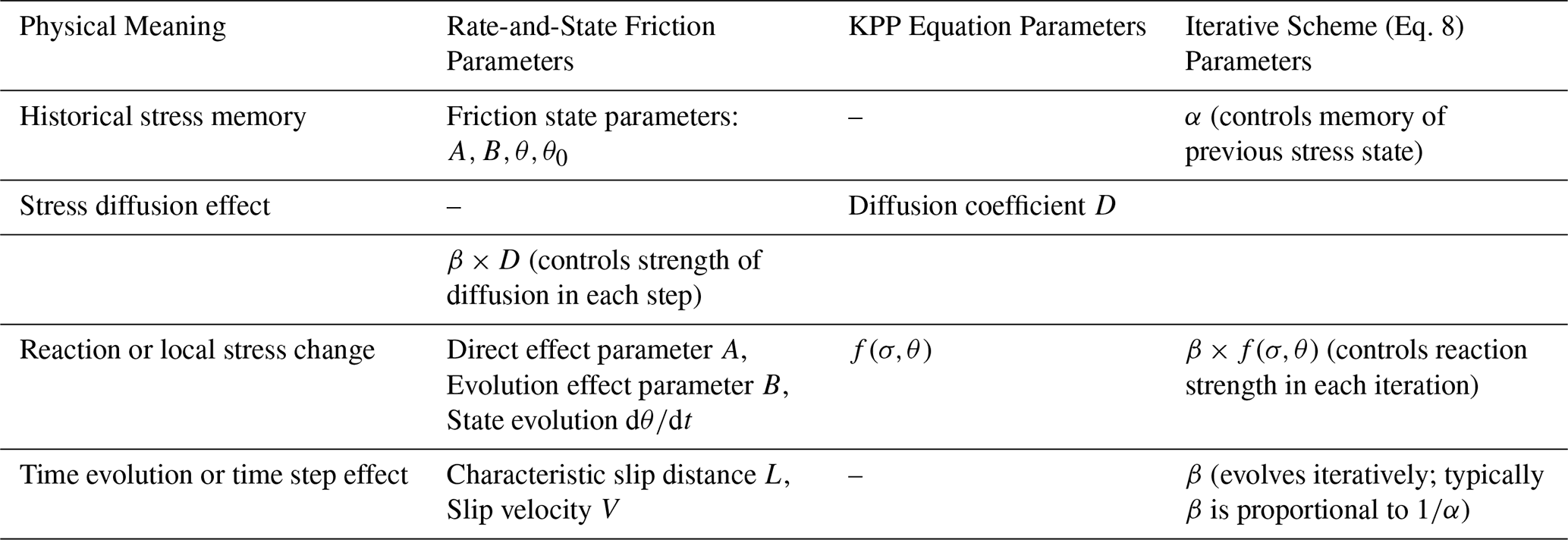
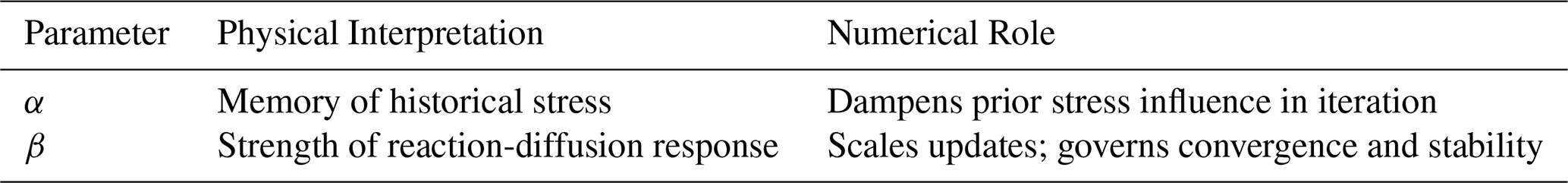
Physically, α captures the persistence of prior stress conditions, analogous to frictional healing effects in fault mechanics. A higher α indicates greater retention of past stress, while a lower α allows rapid adaptation. Conversely, β determines the strength of each update, acting as an effective step size for stress redistribution and state evolution. From a numerical perspective, α acts as a damping factor, preventing abrupt transitions by controlling how much of the prior stress state is retained. Parameter β functions similarly to a relaxation parameter, scaling the response to local perturbations and ensuring convergence under Banach's condition. To clarify their dual roles, we provide Table 2 as below.

Table 2 The physical meanings and numerical roles of the parameters α and β.

In the subsequent numerical simulations, we demonstrate how variations in α and β influence convergence rate and stress field evolution. A balanced choice ensures both stability and efficiency while reflecting the natural damping behavior of crustal stress systems.

2.2 Numerical Stability and Parameter Constraints

The parameters α and β are not treated as tunable material constants nor optimized fitting parameters. Instead, they are interpreted as evolution weights that regulate stress memory and redistribution under admissible numerical and physical constraints. The present framework does not explicitly model fault geometry or discrete fault-controlled interactions. Instead, rupture complexity is incorporated implicitly through the initial stress perturbation derived from elastic dislocation modeling. This 2D stratified approach isolates depth-dependent stress evolution behaviors, avoiding potential biases from over-specifying poorly constrained fault-specific variables while maintaining high fidelity in the computed stress field. Model parameters are selected within an admissible domain defined by numerical stability, boundedness of solutions, and physical consistency with the tectonic environment of eastern Taiwan. Rather than being treated as fixed material constants, the adopted parameters are interpreted as effective parameters that describe the collective response of a heterogeneous fault system at the modeled spatial and temporal scales. The stress-memory parameter (α) controls the persistence of stress heterogeneity during postseismic evolution and is chosen to avoid unrealistically rapid homogenization inconsistent with the prolonged aftershock activity observed following the 2018 Hualien earthquake. Diffusion-related parameters (β) regulate the temporal scale of stress redistribution while remaining secondary to memory effects under the adopted spatial resolution. Reaction parameters are normalized by event-specific stress amplitudes to ensure bounded nonlinear response. Optimizing α–β to minimize forecast error would be physically misleading, as it would conflate numerical convergence control with material property inversion.

The present model adopts an admissible-domain formulation, allowing it to capture sustained, heterogeneous postseismic stress evolution while maintaining numerical convergence and physical interpretability. Within this framework, parameters are interpreted as effective values describing the collective response of a heterogeneous fault system – rather than fixed material constants – providing a transferable approach for diverse tectonic settings without over-specifying poorly constrained properties. To operationalize this, the stress evolution equation is discretized on a 50×50 uniform grid with spatial resolutions of Δx=1320 m and Δy=2600 m (effective length scale Δx_eff=2900 m). This specific configuration, validated through numerical sensitivity tests, represents a practical compromise between resolving near-fault stress-gradient structures and maintaining computational efficiency. The mild spatial anisotropy (Δx<Δy) naturally accommodates the geometric aspect ratio of the study domain and enhances resolution perpendicular to the dominant fault strike, where stress-polarity transitions are sharpest. Crucially, the numerical grid resolution characterizes the fidelity of the computed stress field and must not be interpreted as the spatial resolution of earthquake locations. While hypocentral location uncertainty constrains the scale of physical interpretation, the numerical discretization is governed strictly by the stability and convergence requirements of the reaction–diffusion equations. Accordingly, model performance is evaluated using statistical measures rather than point-wise spatial correspondence, with physical interpretation restricted to spatial scales comparable to or larger than typical location uncertainty.

Furthermore, a critical distinction is maintained between numerical discretization fidelity and observational data uncertainty. While the adopted grid resolution (Δx,Δy) is finer than the typical earthquake location uncertainty (approximately 2–3 km), such a discretization is mathematically necessary to accurately resolve localized stress gradients (∇σ) and diffusion terms (∇²σ) without introducing spurious numerical smoothing. As demonstrated in previous studies (Ziv and Rubin, 2000), although individual hypocentral errors are unavoidable, the resulting stress-triggering patterns and polarity boundaries remain statistically robust. Consequently, the high-resolution grid provides a numerically stable background field, while our physical interpretation of the 2018 Hualien sequence is consistently restricted to spatial scales comparable to or larger than the location uncertainty. This ensures that the model captures the large-scale spatiotemporal evolution of the stress field in a statistically meaningful sense, rather than attempting deterministic cell-by-cell predictions.

The stress diffusion coefficient is set as $D={\mathrm{10}}^{-\mathrm{2}}$ m² s⁻¹, consistent with fluid-assisted or elastic stress propagation in the crust. The corresponding term DC $\sim \mathrm{1}/\mathrm{\Delta }{x}_{\mathrm{eff}}^{\mathrm{2}}\times {\mathrm{10}}^{-\mathrm{2}}$ is approximately to 10⁻⁸, quantifying the smoothing effect of diffusion on the evolving stress field. To satisfy the contraction condition $\mathit{\beta }<\frac{(\mathrm{1}-\mathit{\alpha })}{(\mathrm{DC}+L_f)}$ (Eq. 11), we evaluate the Lipschitz constant of the nonlinear reaction term using the supremum of its partial derivative:

$$\begin{array}{}\text{(12)}& L_f\ge sup\left({\displaystyle \frac{\partial f\left(\mathit{\sigma },\mathit{\theta }\right)}{\partial \mathit{\sigma }}}\right)=sup\left(A\left(\mathrm{1}-\mathrm{2}{\displaystyle \frac{\mathit{\sigma }}{{\mathit{\sigma }}_{max}}}\right)\right)=A_{\mathrm{0}}\end{array}$$

Assuming A₀=0.01, and setting α=0.4 to avoid unphysically rapid stress dissipation, we derive an upper bound for β:

$$\begin{array}{}\text{(13)}& \mathit{\beta }<{\displaystyle \frac{(\mathrm{1}-\mathit{\alpha })}{(\mathrm{DC}+L_f)}}<{\displaystyle \frac{\mathrm{0.6}}{{\mathrm{10}}^{-\mathrm{8}}+\mathrm{0.01}}}\approx \mathrm{60}\end{array}$$

Moreover, numerical diffusion stability is governed by the Courant–Friedrichs–Lewy (CFL) condition, modified for our weighted scheme:

$$\begin{array}{}\text{(14)}& \mathrm{\Delta }t\le {\displaystyle \frac{\mathrm{\Delta }x\mathrm{\Delta }y}{\mathrm{2}\mathit{\beta }D}}\end{array}$$

For β=50, this yields a maximum stable time increment of:

$$\begin{array}{}\text{(15)}& \mathrm{\Delta }t\le {\displaystyle \frac{\mathrm{1320}\cdot \mathrm{2600}}{\mathrm{2}\cdot \mathrm{0.01}\cdot \mathrm{50}}}=\mathrm{3}\mathrm{432}\mathrm{000}\mathrm{s}=\mathrm{39.72}\mathrm{d}\end{array}$$

This duration aligns with the early aftershock window targeted in this study. The selected spatial resolutions were calibrated to balance model accuracy and computational feasibility. A sensitivity analysis with ±20 % variation in Δx and Δy confirmed that our configuration maintains CFL compliance (β upper bound = 95.3 for +20 % and 42.4 for −20 %), validating the stability of our β = 50 setting. While slight variations in grid resolution may impact Coulomb stress gradients and aftershock localization, our preliminary assessments show negligible distortion, supporting the robustness of our chosen setup.

2.3 Critical Iteration Number for Diffusion Dominance

The critical iteration number, n_critical, is defined as the point at which stress diffusion overtakes local stress reaction in driving the evolution of the stress field. The transition from reaction-dominated to diffusion-dominated behavior can be characterized by a simple scaling balance. Assuming σ_n≈σ₀αⁿ, the reaction contribution scales as A₀σ₀αⁿ, while the diffusion contribution scales as D₀Δσ₀. Equating the two yields analytically a critical iteration index

$$\begin{array}{}\text{(16)}& n_{\mathrm{critical}}={\displaystyle \frac{\ln \left(\frac{A_{\mathrm{0}}\mathrm{\Delta }{\mathit{\sigma }}_{\mathrm{0}}}{D_{\mathrm{0}}{\mathit{\sigma }}_{\mathrm{0}}}\right)}{-\ln \left(\mathit{\alpha }\right)}},\end{array}$$

Here, A₀ is the friction parameter, D₀ is the stress diffusivity, σ₀ denotes a characteristic stress amplitude, and Δσ₀ is the initial stress contrast between adjacent grid points. This expression provides an intuitive explanation for depth-dependent differences in stress persistence. Physically, this quantity marks the transition from a reaction-dominated regime (early stress accumulation) to a diffusion-dominated regime (stress homogenization). Assuming D₀≈A₀ for simplicity, Eq. (15) shows that large stress gradients (i.e., high $\mathrm{\Delta }{\mathit{\sigma }}_{\mathrm{0}}/{\mathit{\sigma }}_{\mathrm{0}}$) lead to higher n_critical, particularly at shallow depths where heterogeneity is pronounced. In deeper layers, reduced gradients yield smaller n_critical, allowing stress diffusion to dominate earlier. Thus, this parameter serves as a diagnostic for identifying the timing of dominant physical processes in postseismic stress evolution.

3 Results and Discussions

3.1 Detections of the proposed model

We applied the proposed iterative stress evolution model to the M_w 6.4 Hualien earthquake that occurred on 6 February 2018, at a depth of 10 km in northeastern Taiwan (Fig. 1).

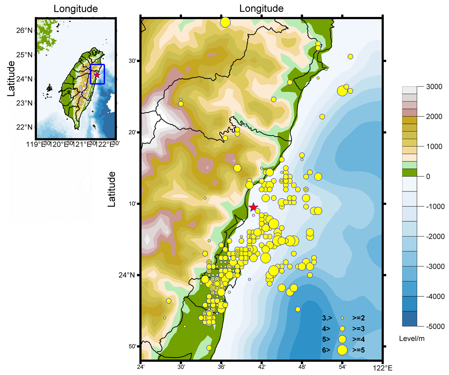
Figure 1 The epicenter of the moderate earthquake that occurred on 6 February 2018 is marked by a red star, while aftershocks ranging from magnitudes 2 to 5 within a three-month period are indicated by yellow circles.

The Hualien M_w 6.4 mainshock occurred in the complex convergence boundary of the Philippine Sea Plate and Eurasian Plate. According to the results of Huang et al. (2019), the Hualien earthquake was likely caused by three faults, with the greatest impact being on the west-dipping fault. This eventually triggered the shallower Milun Fault, leading to surface rupture. Therefore, it is essentially an interplate event, which is consistent with its vigorous aftershock sequence. In the first 12 d alone, over 2100 aftershocks were recorded in the Hualien sequence (Hao et al., 2018), reflecting high aftershock productivity characteristic of plate-boundary earthquakes. The earthquake resulted in 17 fatalities, over 300 injuries, and the collapse of four significant buildings (Nieh et al., 2020)

A key feature of the present framework is its focus on two-dimensional, depth-dependent stress evolution. Accordingly, Fig. 1 defines the study domain and the initial distribution of seismicity, while explicit fault geometries and color-coded focal depths are intentionally omitted to remain consistent with this depth-stratified modeling strategy, which isolates stress evolution within independent horizontal slices instead of resolving fault-specific three-dimensional interactions. The subsurface structures in the Hualien region exhibit significant three-dimensional heterogeneity (Kuo-Chen et al., 2012), these complexities – including focal mechanisms, multi-fault segmentation, and non-planar rupture (Lee et al., 2019) – are incorporated implicitly as the primary driving structure of the model. Specifically, fault geometry and slip distribution are mathematically transformed into a highly heterogeneous initial stress field σ(x,0) through elastic dislocation modeling. From the perspective of reaction–diffusion dynamics, the resulting stress gradients govern the deterministic spatial evolution pathway, whereas variations in material properties (such as crustal permeability or rheology) primarily modulate the temporal scale of redistribution. By assuming a spatially uniform diffusion coefficient D within each horizontal layer, the model isolates the dominant role of stress gradients in controlling postseismic redistribution. Based on prioritizing the high-resolution characterization of stress gradients over poorly constrained 3D structural parameters, the model captures the macroscopic response of complex fault systems while maintaining mathematical uniqueness and stability. Prioritizing high-resolution characterization of initial stress gradients over poorly constrained structural parameters allows the proposed framework to capture the macroscopic response of complex fault systems while maintaining mathematical uniqueness and stability. This methodology ensures that the “physical essence” of the subsurface structure – including non-planar fault geometries and 3D heterogeneities – is preserved within the stress-field topology, even in a depth-stratified 2D formulation. Such an approach aligns with empirical findings (Ziv and Rubin, 2000), which demonstrate that stress-triggering patterns remain statistically robust despite medium uncertainties in the crustal structure. Consequently, the high-resolution stress gradient serves as a reliable deterministic driver for postseismic evolution, effectively bridging the gap between complex geological reality and numerical model interpretability.

Beyond the horizontal complexity, the vertical distribution of the Hualien sequence also provides critical insights into the stress relaxation process. The 2018 Hualien earthquake's aftershocks were mostly confined to mid-crustal depths (∼ 5–15 km) with very few events in the uppermost <5 km. This depth-dependent clustering suggests that the shallow crust (above ∼ 5 km), which in eastern Taiwan includes unconsolidated sediments and fractured rocks near the surface, did not generate many aftershocks. In contrast, the brittle mid-crust (roughly 5–15 km deep) hosted the vast majority of aftershocks, consistent with this depth range being the primary seismogenic zone of strong, brittle rocks (Hao et al., 2018). Near the surface, rocks tend to be cooler, highly fractured, and may contain groundwater or other fluids, all of which promote brittle failure and abundant micro-seismicity.

At greater depths, however, higher temperature and pressure conditions lead to changes in rock behavior. It indicates that in the brittle-ductile transition zone (around the lower crust), pore-fluid pressure build-up can induce slip instability on faults that would otherwise creep stably (Wen et al., 2019). Thus, at about 15–25 km depth, the rock chemistry and rheology (e.g., dehydration of minerals, crystal plasticity) can limit aftershock productivity unless high fluid pressures locally enable brittle failure. In the Hualien sequence, this is reflected by the paucity of aftershocks below ∼ 15 km, suggesting that deeper rocks deform more aseismically. Jian et al. (2018) also showed that there were at least 16 earthquakes with a magnitude greater than 4.5, including one earthquake with a magnitude of 6.1, distributed in the depth range of 3 to 15 km. In addition, shallow aftershocks may decay more rapidly in number due to rapid stress relaxation in brittle, fractured rock, whereas at intermediate depths, the decay could be influenced by fluid diffusion and healing processes in the fault zone. This deviation is likely due to different stress persistence in stronger rocks and possible ongoing creep at depth that dampens prolonged aftershock sequences. In the Hualien sequence, this transition is reflected by the sharp decrease in seismicity below approximately 15 km depth. These observations support the use of depth-dependent modeling parameters and motivate the stratified analysis of postseismic stress evolution adopted in this study.

The corresponding source slip model of the earthquake was derived using co-seismic GPS data recorded near the epicenter and a Genetic Algorithm (GA) inversion technique to calculate Coulomb stress changes at depths ranging from 6 to 30 km (Liao et al., 2024). Building on this research, we use this earthquake as a case study to examine the evolution of Coulomb stress changes across different depths. Before presenting the results, note that our model's stress evolution is driven by two key parameters: α represents the system's memory of prior stress, while β sets the strength of stress diffusion and reaction processes. This physical interpretation helps explain the distinct stress distributions and convergence behaviors observed at different depths. To systematically investigate the impact of parameters α and β introduced in Eq. (9), we conducted a series of parameter sensitivity tests (Figs. 2 and 3). The tested ranges for α (0.5–0.9) and β (1–20) were chosen to satisfy the Banach fixed-point theorem's conditions for convergence and stability. Physically, a larger α means more of the past stress is retained, so more iterations are needed for the solution to converge – analogous to an aftershock sequence that drags on longer in a fault system. Conversely, choosing β at extreme values (too large or too small) can prevent the model from converging. In physical terms, an unrealistic β would correspond to a diffusion speed outside the bounds of rock mechanics observations. For the following analysis, we fix α=0.75 and β=0.7 for initial model runs across various depths to evaluate their effects. Crucially, within this framework, iteration index serves as a dimensionless evolution parameter rather than a direct measure of physical time. Temporal effects are introduced exclusively through the time-dependent memory parameter α(t), which is linked to Omori-type decay, with β(t) adjusted correspondingly to regulate diffusion–reaction balance.

Four parameters – Iterative Time, Maximum Stress Value Evolution, High Residual Stress Area, and Iteration Differences – are used as indicators to evaluate the differences across each depth. The results are presented in Fig. 2.

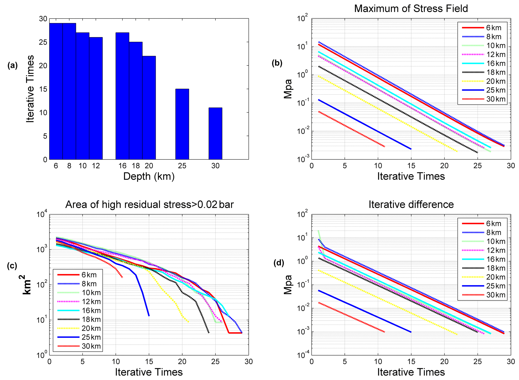
Figure 2 Illustration of iterative convergence and stress field evolution across depths. (a) Iterative counts required for stress field stabilization at different depths. Shallower depths (6–12 km) generally require more iterations, reflecting the higher variability and complexity in stress redistribution at these levels. (b) Maximum stress field magnitude plotted against iteration counts for depths ranging from 6 to 30 km. A consistent logarithmic decay is observed, indicating systematic convergence of the stress field, with deeper layers achieving stabilization more rapidly than shallower ones. (c) Area of high residual stress (> 0.02 bar) versus iteration counts. Shallower depths initially exhibit larger areas of high residual stress, which significantly diminish through iterative updates, consistent with stress redistribution and relaxation processes. (d) Iterative differences in the stress field plotted against iteration counts for various depths. The differences decrease logarithmically, with deeper layers achieving stability faster, reflecting the reduced variability in stress dynamics at greater depths. These visualizations underscore the depth-dependent nature of stress evolution, highlighting the interplay between iterative convergence and stress relaxation. The results provide critical insights into the temporal and spatial dynamics of post-seismic stress fields, emphasizing the importance of depth-stratified modeling for understanding stress redistribution processes.

Based on the chart data, here's a detailed analysis of key findings regarding stress evolution at different depths (6–30 km). The analysis of stress evolution across varying depths in Fig. 2a highlights critical differences in the convergence process of post-seismic stress fields. In shallow layers (6–12 km), the larger initial stress magnitude necessitates over 20 iterations to achieve convergence, as the historical stress term (controlled by α) dominates the redistribution process. In contrast, middle layers (16–20 km) exhibit moderate initial stress values, stabilizing within 10–20 iterations. Deep layers (25–30 km) are characterized by smaller initial stress magnitudes, allowing the stress field to converge in fewer than 10 iterations. These findings demonstrate that the required iterations for convergence are primarily determined by the absolute stress magnitude and are influenced by the initial stress gradient characterized stress transfer at different depths. In shallow layers, larger stress gradients ($\mathrm{\Delta }{\mathit{\sigma }}_{\mathrm{0}}/\mathit{\sigma }$) and localized stress accumulation require more iteration steps to smooth stress fluctuations and achieve a stable state. In contrast, deeper layers exhibit smaller stress gradients and more uniform initial stress fields, allowing faster convergence with fewer iterations as the diffusion term quickly balances stress differences. It is worth noting that the number of iterations does not represent the convergence time. In deeper layers, fewer iterations do not necessarily imply shorter convergence times. For shallow layers, each iteration may correspond to several hours to several days, depending on the combination of α and β values; while in deeper layers, a single iteration may represent several months or even years, depending on the rock conditions at depth.

Further analysis of Fig. 2b shows that the maximum stress values decrease exponentially with increasing iterations, especially in shallow layers with higher initial stress concentrations. This reflects the dominance of the historical stress term (αⁿ) in the evolution process. Since the β value is small, the effects of the diffusion and reaction terms are limited, and changes in the stress field are primarily driven by the gradual decay of historical stress. Figure 2c shows the evolution of high residual stress areas (> 0.02 bar km⁻²), which also highlights depth-dependent characteristics. In shallow layers, the decrease in high-stress areas is slower because the contributions of diffusion and reaction terms are insufficient. Under the dominance of historical stress, stress differences take more time to smooth out. On the contrary, in deep layers, high-stress areas decrease more quickly due to smaller initial stress differences, requiring fewer steps to achieve convergence. Figure 2d demonstrates that with increasing iterations, the differences in the stress field gradually diminish, and the convergence rate is significantly faster in deep layers compared to shallow layers. This fact reveals that stress fields in deeper layers are inherently more uniform, with limited influence from diffusion and reaction terms. Thus, fewer iterations are needed to reach a stable state.

Under the condition of $\mathit{\beta }=\mathrm{0.9},$ the contributions of diffusion and reaction terms to stress evolution are quite small, and the overall evolution is dominated by historical stress. In shallow layers, the larger stress differences require more iterations to converge, while in deep layers, the more uniform stress fields allow for faster convergence.

3.2 Single-factor analysis of parameters

In this section, we conduct a single-parameter analysis of α and β. This parameter-sensitivity test demonstrates that α and β are not arbitrary. Here, α directly controls how long past stress effects persist, whereas β governs the strength of the diffusion–reaction updates. Figure 3a–d confirm how changing α or β shifts the stress field's heterogeneity (STD) and error (MSE), providing insight into the numerical and physical implications of Eq. (9).

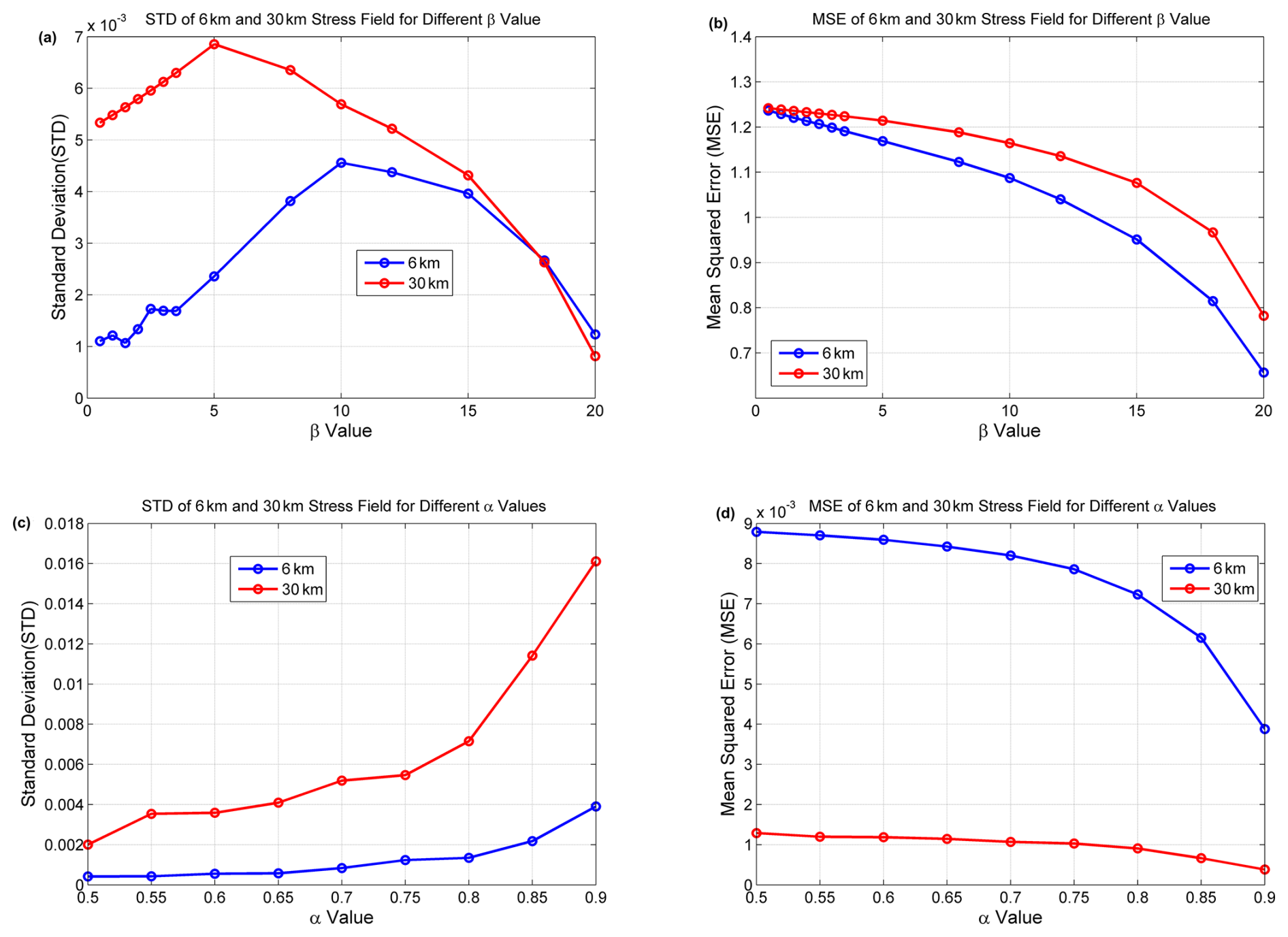
Figure 3 Evolution of Standard Deviation (STD) and Mean Squared Error (MSE) for stress fields at 6 and 30 km depths with varying parameter values of β and α: (a) STD as a function of β (α=0.75): The peak STD is observed at β=10 for 6 km and β=5 for 30 km. Higher β values lead to increased smoothing of the stress field and reduced STD. (b) MSE as a function of β (α=0.75): MSE decreases monotonically with increasing β, as diffusion dominates and smooths the stress field. The MSE is consistently higher at 30 km due to limited smoothing effects from fewer iterations. (c) STD as a function of α (β=10): Larger α values cause the system to release prior stress more slowly, leading to greater stress-field heterogeneity and a higher STD. STD at 30 km is consistently higher due to preserved heterogeneity. (d) MSE as a function of α (β=10): At 6 km, MSE decreases with increasing α, indicating better alignment with theoretical values. At 30 km, MSE remains stable due to consistent diffusion and reaction effects. These results illustrate the interplay between β and α in influencing stress field evolution and the impact of depth on stress redistribution.

In this study, the STD and MSE are employed as internal diagnostic metrics to characterize the evolution of stress-field heterogeneity and numerical convergence, rather than to represent discrete aftershock productivity or event counts. Defined in iteration space, these diagnostics quantify the spatial variability of the continuous stress field under different values of α, β, and depth, enabling consistent comparison of stress redistribution behavior without being interpreted as calibrated physical time. The selected parameter ranges (α=0.5–0.9, β=0.5–20) are adopted to conduct controlled parameter-sensitivity analyses and to characterize stress evolution under admissible regimes, where numerical stability and boundedness are mathematically guaranteed (e.g., α<1 and CFL-type constraints). Accordingly, the parameters α and β are not treated as calibration variables, and the notion of an “optimal” β or (α,β) pair has no physical meaning in the present formulation.

In contrast to empirical measures such as Omori-law decay exponents, which describe temporal variations in earthquake occurrence rates, the diagnostics used here focus on the underlying physical process of stress-gradient dissipation and homogenization. Accordingly, trends in STD reflect the persistence and decay of stress heterogeneity – providing the physical “seed” for delayed triggering – rather than constituting a direct fit to observed seismicity decay curves. Consequently, an explicit two-dimensional scan of the (α,β) parameter space would primarily reproduce the known stability domain, without yielding additional physical insight or refined calibration for real-time PSHA applications, which rely on hazard aggregation rather than internal numerical control parameters. The objective of this study is therefore to demonstrate robust, physically interpretable stress evolution across an admissible parameter domain, rather than to pursue parameter optimization or inversion. According to Eq. (9), α applies a weight to the previous iteration's stress, while β determines the magnitude of the diffusion–reaction term at each step. Therefore, each curve in Fig. 3a–d is directly driven by the interplay between these two scaling factors, validating the underlying Banach-based iterative scheme. First, we fix α=0.75 and vary β from 0.5 to 20 to calculate the standard deviation (STD) and mean squared error (MSE) of different stress evolutions at depths of 6 and 30 km, as shown in Fig. 3a–b. Subsequently, we fix β=0.95 and vary α from 0.5 to 0.9 to analyze STD and MSE, as illustrated in Fig. 3c–d.

Figure 3a has three valuable observations. The first point is STD at 30 km is higher than that at 6 km. This behavior is attributed to several factors: (1) Initial stress is smaller, but convergence requires fewer iterations. At 30 km, the initial stress (σ₀) is smaller, and fewer iterations are needed to meet the convergence criterion. However, fewer iterations mean that the contributions from diffusion and reaction terms are limited, preserving more heterogeneity in the stress field and leading to a higher STD. (2) More iterations are needed at 6 km: At 6 km, the larger initial stress (σ₀) and greater stress difference (Δσ₀) result in more iterations being required for convergence. This allows diffusion and reaction terms to play a greater role in smoothing the stress field, reducing heterogeneity, and yielding a lower STD. (3) Weaker contributions from diffusion and reaction terms at 30 km: At the same β, the effects of diffusion and reaction terms are relatively smaller at 30 km compared to 6 km. As a result, stress heterogeneity persists longer at 30 km, contributing to a higher STD. The fact that at 30 km the STD peaks at β=5, while at 6 km it peaks at β=10, suggests deeper layers reach equilibrium faster under smaller β. This aligns with the idea that deeper faults experience a more uniform stress distribution, hence a lower threshold for diffusion dominance.

The second key point is that STD increases and then decreases with β. At both 6 and 30 km, the STD initially increases with β, reaches a peak, and then decreases. This trend can be explained as follows: (1) For small β, diffusion and reaction contributions to the stress field are quite small, and stress evolution is primarily governed by historical stress, preserving stress heterogeneity. (2) As β increases, the contributions from diffusion and reaction terms grow. However, if the convergence iteration count (n) remains below the critical iteration number (n_critical in Eq. 15), reaction effects dominate, amplifying local stress, leading to an increase in STD. (3) When β becomes large enough to exceed n_critical, diffusion effects dominate, smoothing the stress field and reducing STD. The larger the β, the greater the smoothing effect, resulting in a lower STD.

The final key point is that peak STD occurs at different β values for 6 and 30 km. The peak STD occurs at β=5 for 30 km and β=10 for 6 km. This difference is due to the smaller n_critical at 30 km compared to 6 km. As β increases, both diffusion and reaction contributions to the stress field increase, requiring more iterations for convergence. At 30 km, the smaller n_critical allows diffusion effects to dominate sooner, causing STD to decrease more quickly. Conversely, at 6 km, the larger n_critical delays the onset of diffusion dominance, so STD decreases only after β>10.

Figure 3b demonstrates two important phenomena. The first one is that as β increases, the MSE exhibits a monotonic decreasing trend. When the β value is small, the model is primarily dominated by historical stress evolution, with few contributions from diffusion and reaction terms. These terms, which represent the influence of stress redistribution and spatial diffusion processes, play a crucial role in smoothing the stress field and reducing MSE as the stress field evolves closer to the target state. Finally, diffusion dominates when the β tends to be large, resulting in a highly smoothed stress field where MSE approaches its minimum. The second is MSE at 30 km, which is consistently higher than 6 km. At 30 km, the reduced influence of diffusion and reaction terms due to smaller stress differences and fewer iterations required for convergence preserves more of the initial heterogeneity in the stress field. This leads to a higher MSE than 6 km, where larger stress gradients and more iterations facilitate a more substantial smoothing effect, lowering MSE. Numerically, a larger β speeds up diffusion updates but can risk overshoot if too significant; physically, β corresponds to how rapidly stress redistributes in a reaction-diffusion sense. Similarly, a higher α retains historical stress longer, echoing the Rate-and-State concept where past slip is not instantly forgotten, but also potentially lengthens the time to converge to a stable stress field.

Figure 3c highlights an intriguing observation: the STDs for both 30 and 6 km depths increase as α grows, with β fixed at 0.95. A larger α value indicates slower decay of historical stress, allowing more historical stress to influence the stress field evolution, as shown in Fig. 2. This increases heterogeneity and results in a higher STD. Conversely, a smaller α leads to rapid decay of historical stress, stabilizing the stress field more quickly and producing a lower STD. The “Rate-and-State concept” refers to a theoretical framework in geophysics that describes the evolution of frictional strength on fault surfaces. Although the contributions of diffusion and reaction terms to the stress field are relatively small, their impact is greater at 6 km compared to 30 km. This means the stress field at 6 km is smoother than at 30 km, leading to a lower STD at 6 km than at 30 km.

Figure 3d shows that as α increases, the MSE at 6 km decreases, while the MSE at 30 km remains relatively stable. The small α indicates historical stress decays rapidly, with limited contributions from diffusion and reaction terms. This results in a larger discrepancy between the stress and target fields, leading to higher MSE. The large α corresponds to historical stress and decays more slowly, retaining more stress over time. This results in more minor deviations from the target theoretical values, reducing the MSE. However, the slower decay does not necessarily imply a smoother stress field but rather a closer match to the expected theoretical state. At 30 km, the MSE remains stable, likely because the effects of the reaction and diffusion terms are relatively consistent at larger scales, and the influence of historical stress exhibits less variation, implying the MSEs are smaller than those in 6 km. Figure 3 clearly illustrates that as β increases from 1 to 10, the computed stress field progressively smoothens, aligning well with the physical intuition of stress diffusion effects described by the KPP formalism. The correspondence between parameters (α, β) in Eq. (9) and those in the Rate-and-State friction law (R-S) and the KPP reaction-diffusion equation is that the parameter α can be viewed as an extension of the frictional decay coefficient inherent to R-S frictional behavior, reflecting how rapidly the influence of past stresses decays over time. Similarly, the parameter β is proportional to the reaction and diffusion terms in the KPP framework, determining the intensity of local stress reactions and spatial diffusion processes, as illustrated well.

3.3 The Coulomb stress changes evolutions of different depths

The Coulomb stress change acting on the target failure plane is denoted as Eq. (1). The Eq. (1) means shear stress increases (Δτ>0) and/or normal stress decreases (Δσ_n<0, unclamping) will make ΔCFF positive, promoting fault failure, whereas the opposite (shear stress decrease or added normal stress clamping) makes ΔCFF negative, inhibiting failure. In short, positive ΔCFF indicates a region where aftershocks are more likely, and negative ΔCFF (a stress shadow) indicates where they are less likely. If the mainshock causes a fault patch to experience a decrease in normal stress (unclamping of the fault plane), the term −μΔσ_n becomes positive, effectively increasing the Coulomb stress and bringing the fault closer to failure. This means even a small shear stress increase can trigger an aftershock when the fault is unclamped. Conversely, if normal stress increases (clamping), it raises the frictional resistance (μΔσ_n) positively, thus subtracting from Δτ, reducing ΔCFF and making aftershock triggering less likely. According to the Okada (1985) elastic dislocation model, surface deformation and strain fields are derived from the spatial derivatives of displacement, which in turn depend on the distance between the observation point and the dislocation source. Mathematically, these displacement fields decay with distance as inverse-square or inverse-cube functions of the radial distance. As fault depth increases, the observation point becomes more distant from the source, leading to a rapid decay in both shear and normal stress changes due to this geometric attenuation. Physically, this means that deeper faults have a more diffuse and weaker influence on the near-surface stress field, thereby reducing the effectiveness of Coulomb's stress transfer in triggering aftershocks. This depth-dependent attenuation is consistent with both theoretical expectations and empirical observations, where shallow events tend to exhibit stronger aftershock clustering due to higher near-surface stress perturbations.

Based on the above discussion, after understanding the method and the roles and limitations of the parameters α and β, this method in this section focuses on analyzing activities of aftershocks at different depths of the 2018 Hualien earthquake (M_w 6.4). By combining the parameters α and β with Coulomb's stress changes and their corresponding stress gradients, we aim to evaluate the method's capability to assess aftershock activity. Unlike conventional numerical schemes that assume a fixed physical time per iteration, our model employs a non-uniform temporal evolution governed by the functions α(t) and β(t). This design reflects the well-known empirical behavior of aftershock sequences: aftershocks are densest in the early hours and days following a mainshock, then decay rapidly in frequency – a pattern captured by Omori's Law. Based on the results of Sect. 3.2, it indicates that the characteristics of α, a more considerable α, results in a slower stress field evolution, which allows for capturing more aftershock activity. Conversely, a smaller α leads to faster stress evolution but predicts weaker aftershock activity. To emulate this, α(t) is defined to decay inversely with time, that is, α(t) is defined as $\mathit{\alpha }\left(t\right)=\mathrm{1}/(\mathrm{1}+t/\mathrm{49})$, where t denotes the physical time in days since the mainshock. This ensures that early-stage stress retains strong memory of the mainshock, enhancing sensitivity to residual high-stress regions and accurately capturing early aftershock clustering. Conversely, β(t) is modeled as a growing function of time to reflect the increasing dominance of diffusion and relaxation over time. Physically, this implies that as time progresses, the stress field becomes smoother and more homogenized due to widespread redistribution and local reaction mechanisms. Hence, instead of associating one iteration with one unit of time, we allow α(t) and β(t) to encode temporal dynamics implicitly. This approach captures the nonlinear, scale-dependent nature of postseismic stress evolution far more realistically than uniform time-stepping, and aligns with observations that early stress perturbations dissipate faster, while later evolution is dominated by gradual diffusion and healing. Therefore, the parameter β(t) initially represents a relatively smaller scaling factor for diffusion and reaction effects, with its influence progressively increasing as time advances. Thus, we define β(t) as $\mathit{\beta }\left(t\right)={\mathit{\beta }}_{\mathrm{0}}\cdot [\mathrm{1}/\mathit{\alpha }(t\left)\right]$. This reciprocal relationship between α and β ensures that as the fault system's memory of historical stress decreases over time (smaller α), the influence of diffusion and local reaction processes correspondingly increases (larger β). Such a design is physically meaningful, allowing a gradual transition from a history-dominated stress regime at the beginning toward a diffusion-and-reaction-dominated regime at later times. This approach also helps ensure numerical stability and convergence in our iterative numerical scheme. The final value of β must be constrained by the convergence conditions of the fixed-point theorem (Eq. 13) and the CFL condition (Eq. 14). To satisfy these mathematical and physical constraints simultaneously, the scaling constant β₀ is set to 20.

The parameters α and β are constrained within an admissible domain that ensures both numerical stability and physical consistency with the tectonic setting of eastern Taiwan. Specifically, the stress-memory parameter α is calibrated to reflect the delayed mechanical relaxation characteristic of the Taiwan orogenic belt, where high geothermal gradients and rapid tectonic loading promote prolonged stress memory rather than instantaneous release. Similarly, the diffusion-related term βD and the nonlinear reaction term f(σ,θ) are scaled to represent effective stress redistribution within a highly fractured crust and dense fault network. Fixed values of α or β are therefore employed as diagnostic probes to isolate individual parameter effects, whereas the time-dependent coupling – where α(t) decays following Omori-type behavior and β(t) scales reciprocally – is explicitly implemented in the temporal stress evolutions. By maintaining all parameters within a subcritical admissible regime, the framework bridges mathematical well-posedness with geological realism, while remaining generalizable to other tectonic settings through recalibration of the admissible domain rather than modification of the governing equations.

We segmented the aftershock records from the 180 d following the mainshock to examine the method's feasibility. Since the aftershock activity follows Omori's law (Baranov et al., 2022), with more aftershocks occurring shortly after the mainshock, the records were divided into several intervals to evaluate the dense seismic activity. The intervals are as follows: every six hours for the first three days after the mainshock, every 12 h from days 3–7, every three days from days 7–21, every five days from days 21–41, and every 10 d from days 41–51. After day 51, as the aftershock activity became sparse, the intervals were set to every 30 d, continuing until day 180.

Figure 4 illustrates the stress evolution and the distribution of aftershock epicenters over time at a depth of 6 km.

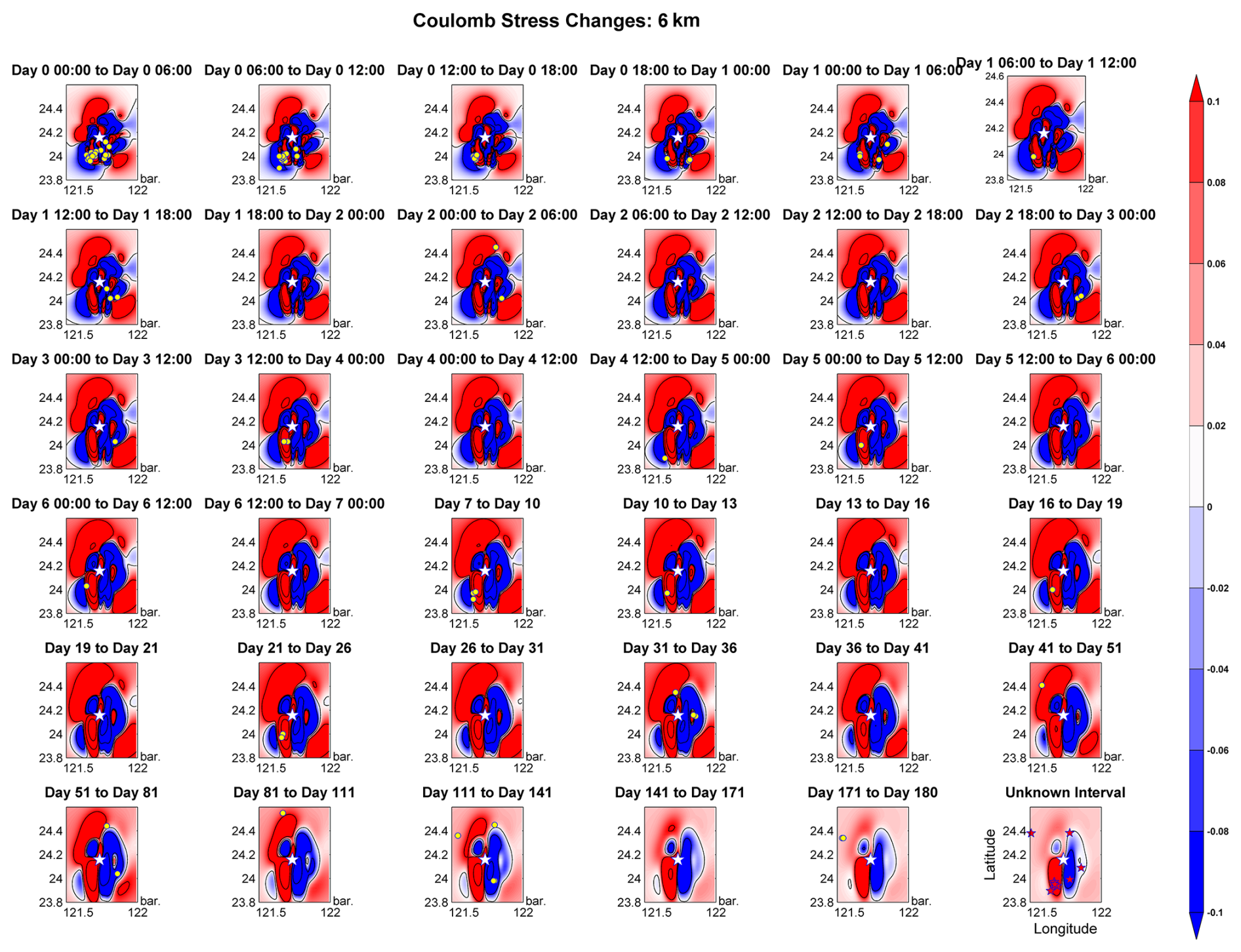
Figure 4 Temporal evolution of Coulomb stress changes at a depth of 6 km during the first 180 d following the 2018 Hualien earthquake (M_w=6.4). Each panel represents the Coulomb stress changes distribution over specific time intervals, with red regions indicating positive stress changes (stress loading) and blue regions indicating negative stress changes (stress unloading). The contours highlight the areas (>0.1 bar) of significant stress concentration. The yellow circles indicate the epicenters of aftershocks occurring within 180 d of the mainshock, while the red stars in the final panel represent those occurring 2 to 3 years after the mainshock.

According to previous studies, Coulomb stress changes exceeding 0.1 bar are more likely to trigger earthquakes (Liao and Huang, 2016; Yang et al., 2024). Therefore, 0.1 bar is considered as the threshold. Based on the results shown in Fig. 4, the following observations can be obtained. At first, in the aspect of distribution characteristics of coulomb stress changes, there are three key points valuable to discuss. (1) The Coulomb stress distribution reveals distinct positive and negative stress regions surrounding the earthquake source. Red areas indicate regions of increased positive stress, while blue areas represent regions of stress unloading (negative stress). (2) Positive stress regions significantly influence the distribution of aftershocks, especially during the first few days following the mainshock. (3) The clear boundaries between positive and negative stress regions suggest that the main rupture surface likely extended along the NE-SW direction, consistent with the typical tectonic trend in the Taiwan region. Furthermore, the slip direction may involve either right-lateral or left-lateral motion along an E–W direction, which is approximately perpendicular to the boundary separating the positive and negative stress zones. This observation aligns with the findings of Huang and Huang (2018), which propose a south-dipping offshore fault connecting to the main west-dipping oblique fault. The second is about the temporal evolution of stress changes, including three characteristics: (1) Over time, the boundaries of positive stress regions expand, highlighting the significant role of stress diffusion processes. (2) Around 50 d after the earthquake, the stress field changes stabilize, suggesting a gradual weakening of the contributions from diffusion and reaction terms. (3) Beyond 50 d, the positive stress regions begin to contract, indicating that aftershock activity is gradually migrating outward and diminishing over time.

The stress field shown in Fig. 4 is converted into stress gradients and displayed in Fig. 5.

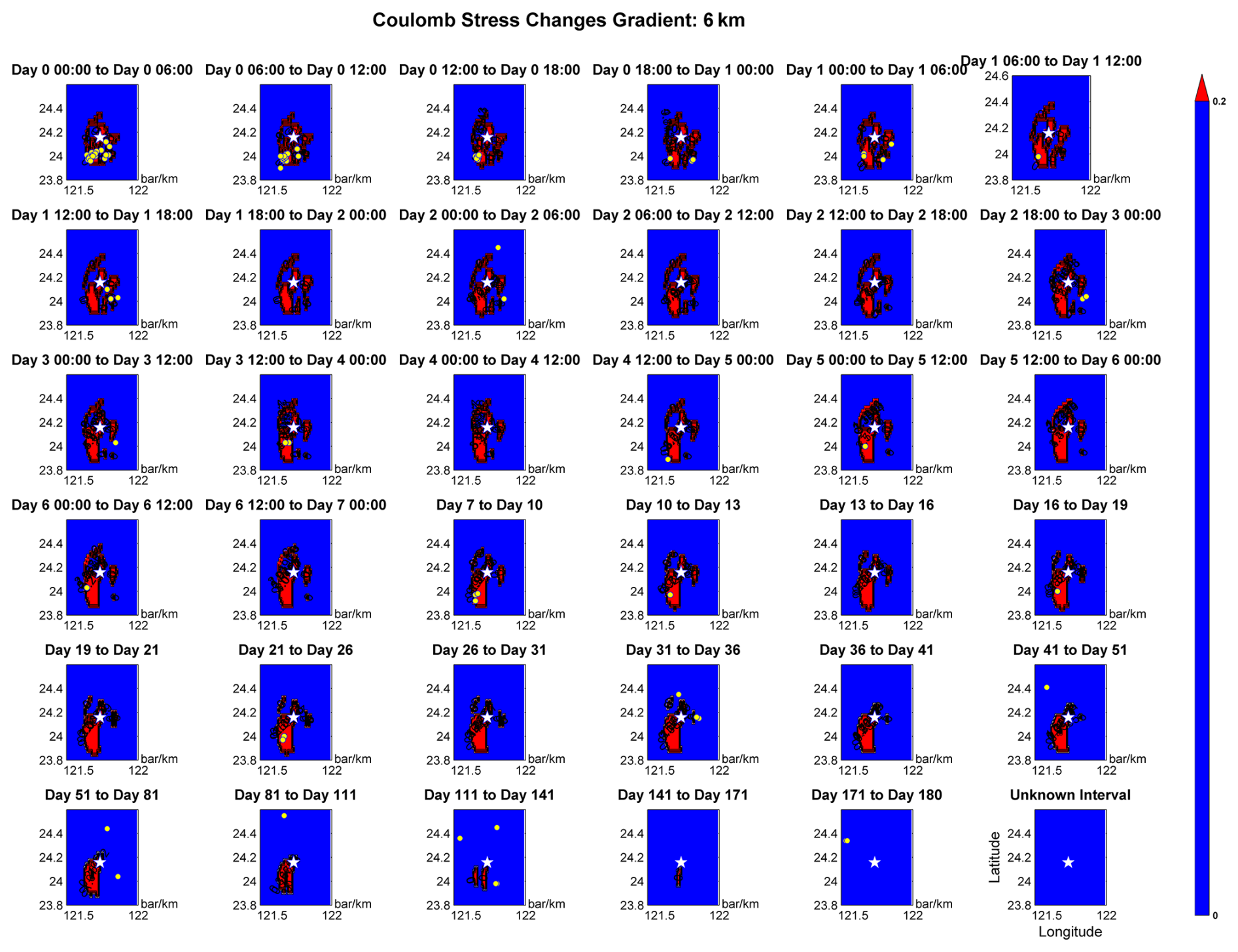
Figure 5 Temporal evolution of Coulomb stress changes gradients at a depth of 6 km during the first 180 d following the 2018 Hualien earthquake (M_w 6.4). Each panel illustrates the distribution of stress gradients (in bar km⁻¹) over specific time intervals. Regions with high stress gradients (> 0.2 bar km⁻¹) are marked in red, while blue areas represent negligible gradients.

The stress gradient is utilized to estimate the occurrence of earthquakes of varying magnitudes across different tectonic settings (Zaccagnino and Doglioni, 2023). The gradient threshold for evaluating aftershocks is set at 0.2 bar km⁻¹, based on the average value of the Youden Index from the AUC analysis. Several key observations can be drawn from Fig. 5. The first one is before 50 d post-earthquake, there is a strong correlation between the locations of aftershocks and regions with high stress gradients, making stress gradient a reliable indicator for predicting aftershock locations. The second is that compared to stress magnitude, stress gradient narrows the focus to smaller regions, improving the accuracy of aftershock prediction. In Fig. 4, stress magnitude shows two high-stress zones northwest and southeast of the epicenter, where aftershocks are scarce. However, in Fig. 5, the stress gradient in these same regions is nearly zero due to the uniformity of the stress field. This highlights that stress gradient, rather than stress magnitude, is likely the driving factor for aftershock activity after the mainshock. Finally, over time, around 50 d post-earthquake, stress gradients gradually stabilize, reflecting the diffusion effect that homogenizes high-gradient areas near the source. As a result, the correlation between stress gradients and aftershock locations diminishes over time. These findings underscore the importance of stress gradients in understanding the mechanisms driving aftershock activity, particularly in the early stages following a mainshock.

Figures 6–7 present the Coulomb stress changes and corresponding stress gradients at a depth of 18 km.

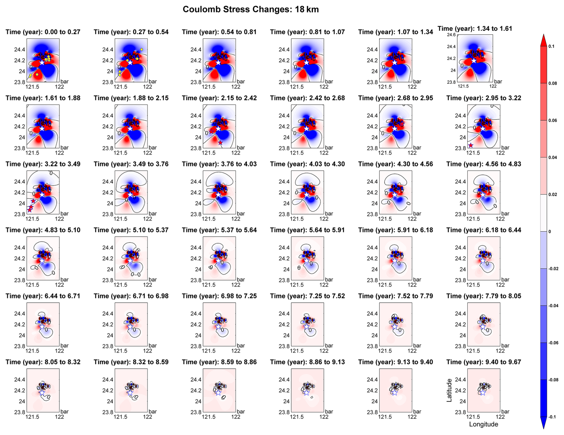
Figure 6 This figure shows the Coulomb stress changes at a depth of 18 km over time, spanning from the mainshock to nearly 10 years post-event. The color represents stress changes, with red indicating increased positive stress and blue denoting stress unloading (negative stress). Yellow circles represent aftershock epicenters occurring within 180 d after the mainshock, while red stars denote aftershocks occurring 2 to 3 years later. The temporal evolution highlights stress changes and redistribution patterns, with stress changes diminishing and stabilizing over time. Notably, aftershock activity correlates strongly with regions of positive Coulomb stress changes during the initial years following the earthquake.

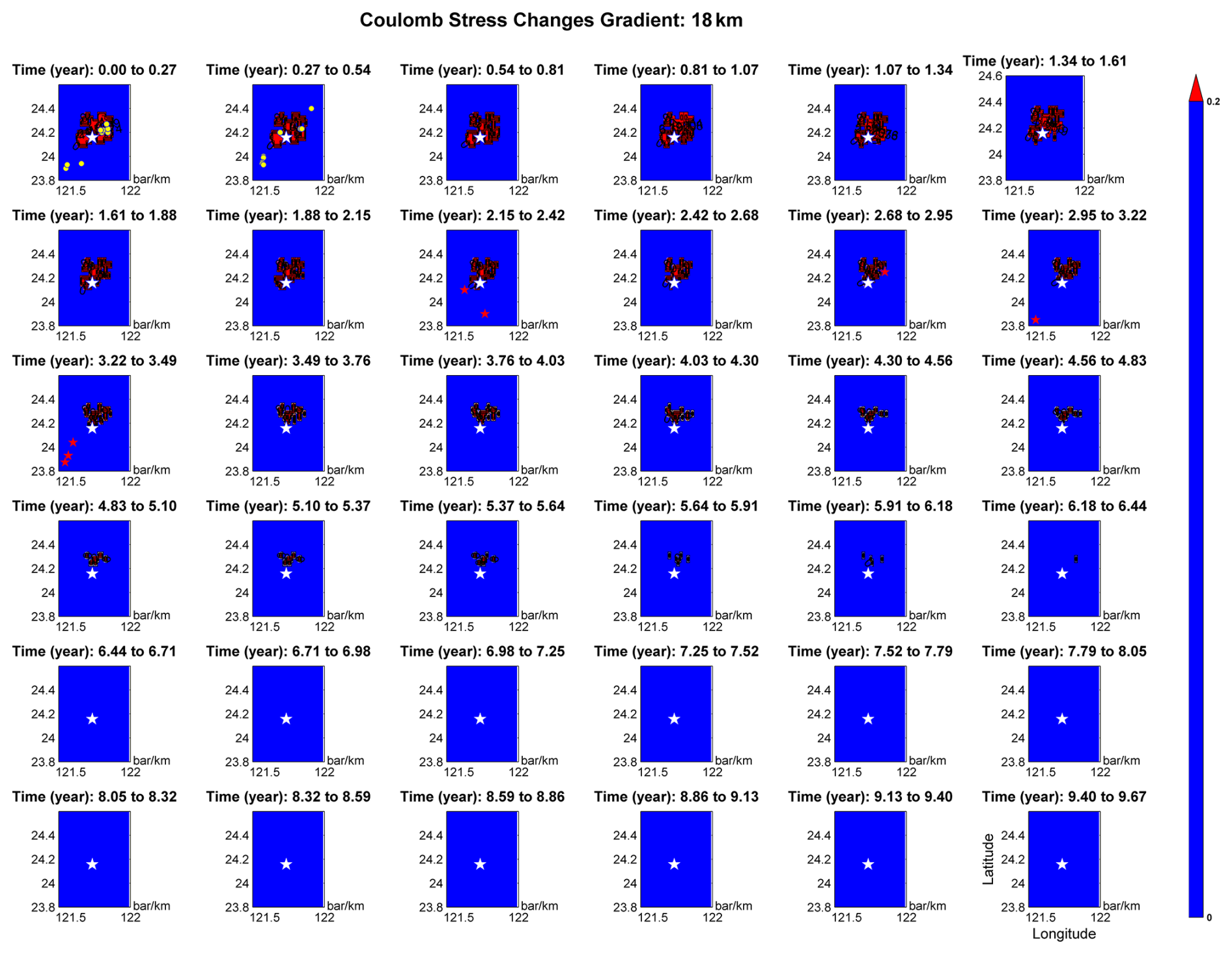
Figure 7 This figure presents the evolution of Coulomb stress gradients at a depth of 18 km over a time span of nearly 10 years following the mainshock. The color scale represents the magnitude of stress gradients, with red highlighting high-gradient zones and blue indicating regions of minimal stress gradient. Yellow circles correspond to aftershock epicenters recorded within 180 d post-mainshock, while red stars signify aftershocks that occurred 2 to 3 years later. The temporal progression illustrates that high-gradient regions correlate with early aftershock activity, but these gradients diminish and stabilize over time due to stress redistribution and diffusion. This stabilization reduces the correlation between stress gradients and aftershock locations in the later years.

For the 18 km depths, the limited number of aftershocks and deviation from Omori's law, along with distinct rock properties compared to shallower layers discussed in Sect. 3.1, necessitate the use of prior studies (Hirth and Kohlstedt, 2003; Shebalin and Narteau, 2017; Hsu et al., 2018) to approximate the time required for stress evolution. The coupled parameters (α,β) are set as (0.8, 10) in the method at depth 18 km. Based on the number of iterations, we calculate the average evolution time for each stage. According to the results of Figs. 6 and 7, there are some excellent findings to discuss. At first, in Fig. 6, multiple time slices during the first 1–2 years following the mainshock (particularly at 0–2.95 years) reveal a distinct pattern of positive Coulomb stress changes (in red) radiating outward from the epicenter in a four-quadrant configuration. This pattern is consistent with the theoretical static stress transfer field generated by shear faulting. Notably, the early aftershocks (yellow circles, within 180 d) are predominantly located within these stress-increased zones, indicating that static stress loading likely facilitated aftershock activity in these areas. The second, during the intermediate stage, approximately 2.95–6 years after the mainshock, the overall magnitude of Coulomb stress changes gradually diminishes, as shown in Fig. 6. Nevertheless, several delayed aftershocks (red stars) still occur within regions of weakly positive stress. Concurrently, Fig. 7 indicates that stress gradients (∇CFF) remain focused around the mainshock fault, suggesting that although the background stress field is decaying, localized stress gradients persist and may still be sufficient to trigger delayed aftershocks. By about six years after the mainshock, the Coulomb stress field becomes largely smoothed and approaches background levels (Fig. 6), accompanied by a pronounced reduction in aftershock activity. Consistent with this evolution, high-gradient zones in Fig. 7 have markedly contracted, leaving only faint remnants near the epicentral region.. This indicates that postseismic stress diffusion and dissipation are nearly complete, aligning with the observed decline in seismic activity. At this stage, spatial stress gradients appear insufficient to drive further ruptures, supporting the view that postseismic stress-triggering effects are time-limited. Finally, while positive Coulomb stress changes (ΔCFF > 0) are effective in predicting early aftershock locations, the stress gradient field provides additional, more sensitive indicators of triggering potential during the early postseismic phase, particularly in areas of strong local stress contrasts. In other words, gradient variations reflect differential slip potentials between adjacent regions, making them a more refined indicator of instability than stress magnitude alone. To conclude, it offers that zones of high stress gradient show strong spatial correlation with early aftershocks, supporting the hypothesis that stress heterogeneity is a key triggering mechanism and stress gradients serve as effective indicators of aftershock triggering potential, offering better spatial resolution than Coulomb stress changes alone, even though stress-driven triggering effects have a limited temporal window.

To quantitatively validate the predictive performance of the model, we utilized Area Under the Curve (AUC) values derived from Receiver Operating Characteristic (ROC) curves analysis, in line with suggestions from previous studies (Fawcett, 2006). An AUC > 0.5 indicates that the classifier performs better than random guessing, validating the model's predictive capability. We further employ the Molchan Area (MA) (Molchan, 1990; Han et al., 2020) to assess the spatial–temporal efficiency of aftershock predictions. The MA explicitly illustrates how effectively our model concentrates predictions into smaller alarm areas while successfully capturing most observed aftershocks. The results of AUC and MA applied to depths of 6 and 18 km are demonstrated in Figs. 8 and 9.

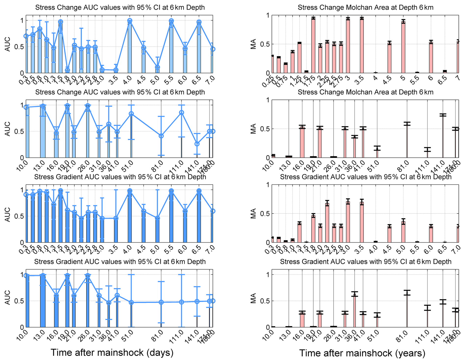
Figure 8 Temporal evaluation of aftershock forecasting performance at 6 km depth using Coulomb stress change (ΔCFF) and stress gradient (∇CFF) metrics. Left panels show the Area Under the ROC Curve (AUC) with 95 % confidence intervals for stress change (top two rows) and stress gradient (bottom two rows), plotted over time after the mainshock (in days). Higher AUC values indicate better performance in distinguishing aftershock locations from non-aftershock areas. Right panels present the corresponding Molchan diagram misfit area (Molchan Area, MA), where lower values indicate higher forecast skill. Each row pair compares AUC (left) and MA (right) metrics for the same input (stress change vs. gradient), allowing direct assessment of their relative performance over different postseismic periods. Notably, both ΔCFF and ∇CFF exhibit high AUC and low MA in the early days following the mainshock, with performance decaying over time. The stress gradient shows slightly improved sensitivity in intermediate periods, suggesting that gradient-based indicators may provide complementary insights into delayed aftershock triggering potential.

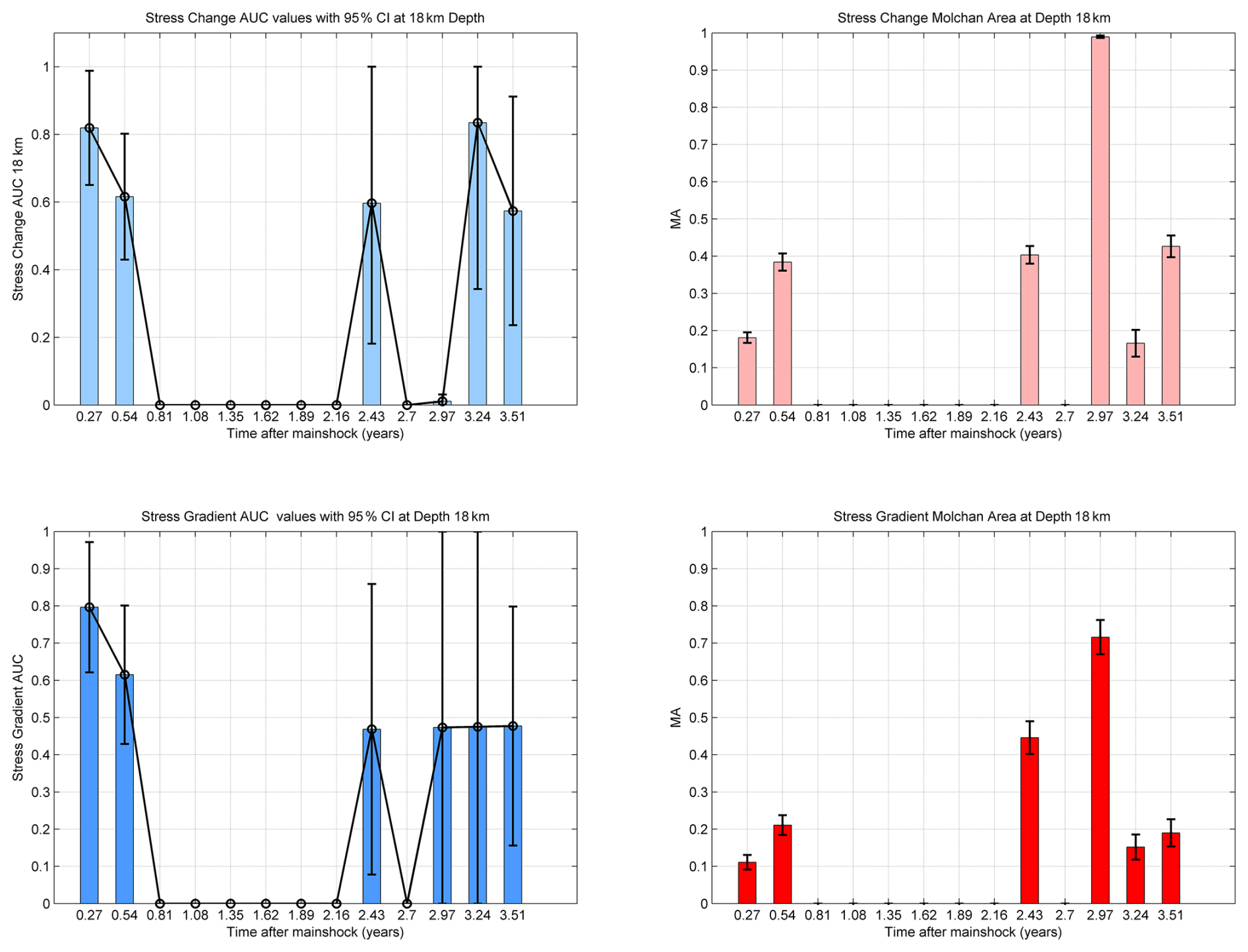
Figure 9 Aftershock forecast performance at 18 km depth using Coulomb stress change (ΔCFF) and stress gradient (∇CFF) over 3.5 years following the mainshock. Left panels show the Area Under the ROC Curve (AUC) with 95 % confidence intervals for ΔCFF (top left) and ∇CFF (bottom left), indicating the model's ability to distinguish between aftershock and non-aftershock regions. Right panels display the corresponding Molchan Area (MA) values (ΔCFF: top right; ∇CFF: bottom right), where smaller values indicate better spatial prediction performance. The early postseismic period (0.27–0.81 years) yields moderate to high AUC values (∼ 0.7–0.8) and relatively low MA values (< 0.3), suggesting that both ΔCFF and ∇CFF maintain forecasting ability at depth during this interval. However, from ∼ 1.0 to 2.7 years, both AUC and MA deteriorate sharply, indicating a loss of predictive power. Partial recovery is observed beyond ∼ 3.0 years in both indicators, but with larger uncertainties.

For examining the spatiotemporal effectiveness of Coulomb stress change (ΔCFF) and its spatial gradient (∇CFF) in aftershock forecasting, we evaluated model performance at two representative depths – 6 and 18 km – using AUC and MA metrics. At 6 km depth (Fig. 8), both ΔCFF and ∇CFF showed robust predictive skill during the first 180 d post-mainshock, with AUC values consistently above 0.7 and MA values below 0.3. The stress gradient (∇CFF) often outperformed ΔCFF in terms of both magnitude and temporal stability, suggesting it captures finer-scale heterogeneity and is more sensitive to local variations in fault stress. These results affirm that shallow stress perturbations are strongly coupled with near-surface aftershock distributions and that ∇CFF serves as a powerful complementary predictor. At 18 km depth (Fig. 9), initial forecasting performance was moderate in the early period (0.27–0.81 years), but a complete loss of predictability occurred between approximately 0.87 and 2.1 years, where AUC values dropped to zero and MA values approached one. Importantly, this is not necessarily indicative of model failure. Instead, our aftershock catalog confirms that no aftershocks were recorded at this depth interval during this time window, precluding the computation of ROC statistics and thus resulting in undefined or default-zero AUC values. This highlights an important limitation in performance evaluation under data scarcity, where the absence of seismicity can mask the model's underlying validity.

Beyond 2.7 years, a partial recovery in forecast performance is observed at 18 km depth, particularly in the ∇CFF metric, where AUC values rebound and MA declines. This may correspond to reactivation of deep fault structures or the emergence of delayed stress-driven instabilities. However, the associated error bars are wide, suggesting increased uncertainty and lower statistical confidence during the late postseismic phase. Comparing both depths, we find that stress-based models perform significantly better in the shallow crust, where stress changes are more concentrated, spatial gradients are sharper, and stress coupling with the aftershock layer is stronger. Deeper sources, by contrast, experience rapid attenuation of stress influence and limited aftershock triggering beyond the early postseismic stage. The consistent strength of ∇CFF at shallow depths further emphasizes the value of incorporating spatial derivatives of stress to resolve high-contrast zones that are not always apparent in absolute ΔCFF fields. These results reinforce the notion that aftershock triggering is both depth- and time-sensitive, and that gradient-based indicators are especially informative under near-field and early-postseismic conditions. Future forecasting models should integrate stress amplitude, stress gradient, and depth as joint predictors to more accurately identify evolving zones of seismic potential.

The AUC results are integrated into Fig. 10 to enable a comprehensive comparison of stress changes and stress gradients across various depths. Additionally, Cohen's d effect sizes were calculated to evaluate the practical significance of differences between stress-based and gradient-based predictions.

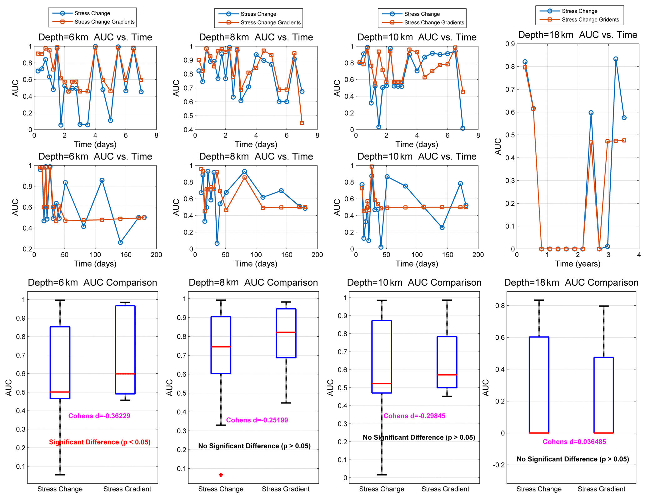
Figure 10 This figure compares the Area Under the Curve (AUC) metrics for stress changes and stress gradients across different depths (6, 8, 10, and 18 km) over time, highlighting their predictive performance for aftershock locations. The lower panels present statistical comparisons of AUC values for each depth, including Cohen's d effect sizes. At 6 km, there is a significant difference (p<0.05) between the two metrics, with stress gradients demonstrating a small effect size advantage (Cohen's d=0.36229). At 8, 10, and 18 km, no significant differences are observed between the two metrics, with minimal effect sizes. These findings suggest that stress gradients are more effective in the short term and at shallower depths, whereas stress changes become more relevant at greater depths and over extended periods.

It should be noted that the spatial distribution of aftershocks – such as the observed higher productivity in the offshore region compared to the onshore area – reflects a combination of stress triggering, fault maturity, and structural heterogeneity. In this study, the depth-resolved stress maps (Figs. 5–7) are not intended as deterministic, point-wise predictors of individual aftershocks, but rather as representations of the time-evolving stress architecture. Consistent with the probabilistic nature of Coulomb stress triggering (Ziv and Rubin, 2000), aftershock occurrence is evaluated based on statistical preference for stress-enhanced or high-gradient regions rather than exact spatial coincidence. To move beyond subjective visual inspection, we employ Area Under the Curve (AUC) analysis (Fig. 10) to quantitatively assess the predictive power of stress changes and gradients. The results indicate that while no single metric is universally optimal, stress gradients exhibit significantly higher sensitivity to aftershock triggering at shallower depths (∼6 km), where structural complexity is pronounced. As depth increases and the stress field becomes smoother, the performance of cumulative stress changes converges with that of gradients. This depth-dependent behavior demonstrates that the model captures the essential physical transitions in the seismogenic zone, providing a statistically robust framework that outperforms random expectations despite inherent observational uncertainties

To further analyze the differences, a paired-sample t-test is employed to evaluate the statistical significance between the AUC values of stress and stress gradients. Cohen's d is additionally used to quantify the effect size of these differences. From Fig. 10, several key insights can be derived regarding the relationship between stress changes, stress gradients, and aftershock prediction at various depths:

1. Initial Observations (First Few Days). In the first few days after the earthquake, AUC values for both stress changes and stress gradients fluctuate significantly, reflecting dynamic aftershock activity and rapidly evolving stress fields. During this period, aftershocks are concentrated in areas of high stress or steep stress gradients, leading to localized but intense seismic activity.

2. 6 km Depth. At a depth of 6 km, the AUC values for stress changes and stress change gradients differ significantly. However, the statistical effect size (Cohen's d=0.36) is less than 0.5, indicating only a small effect. In seismological applications, a “small” Cohen's d (e.g., 0.3–0.5) may still indicate meaningful model discrimination, especially when supported by robust spatial clustering of aftershocks and favorable AUC values. While the Cohen's d value of 0.36229 at 6 km depth falls within the conventional range of a “small” effect size (Cohen, 1988), its operational significance in the context of aftershock forecasting warrants further discussion. This d value represents a standardized difference in AUC between the stress-gradient model and the stress-change model, with the former consistently yielding higher predictive accuracy at early post-seismic intervals. The result indicates that although the improvement is modest in statistical magnitude, it is systematic and physically meaningful, particularly in shallow crustal regions where stress heterogeneities and rupture nucleation are more sensitive to gradients than absolute stress magnitudes. Moreover, in a threshold-sensitive, nonlinear triggering system, such as that for earthquake aftershocks, even small improvements in predictive discrimination can enhance the reliability of alert zones and reduce missed hazard regions. Thus, the d=0.36 should be interpreted not merely as a statistical artifact, but as empirical support for the added value of gradient-based modeling at shallow depths. When interpreted alongside complementary metrics such as Molchan Area and AUC itself, this effect supports the hypothesis that the gradient-based model provides a modest but consistent gain in spatial discrimination of aftershock zones, which represents an effect that is statistically small, but practically meaningful under the operational demands of seismic hazard mitigation. Within the first seven days after the earthquake, the AUC for stress changes (averaged value = 0.60) exhibits greater fluctuations compared to stress change gradients (averaged value = 0.72). Despite this, stress change gradients consistently outperform stress changes in terms of predictive capability.

3. 8–10 km Depth. At depths of 8–10 km, while no statistically significant differences are observed between the two measures, some noteworthy patterns emerge. The average AUC for stress changes at a depth of 8 km during the first seven days after the mainshock is 0.81, while the AUC for stress change gradients is 0.86. At 10 km, the corresponding AUC values are 0.67 and 0.75, respectively. Nevertheless, the AUC values for stress change gradients are not consistently greater than those for stress changes. At 8 km, the AUC for stress gradients is lower than that for stress changes on the 5th and 7th days. Similarly, at 10 km, this phenomenon persists continuously from the 5th to 6th days. This could be attributed to the smoother stress changes at greater depths, which reduce the predictive effectiveness of stress gradients. However, from 7 to 50 d post-earthquake, the AUC differences between stress changes and stress gradients at 6–10 km gradually diminish. Beyond 50 d, stress gradients smooth out to an AUC value of 0.5, losing their ability to predict aftershock locations. These findings align with the observations in Figs. 5, 7, and 9. Regions with high stress gradients shrink over time, and aftershock distributions gradually shift away from these zones of high gradient.

4. 18–25 km Depth. At a depth of 18 km, while AUC values for stress changes and stress gradients show no significant differences, stress changes consistently outperform stress gradients in predicting aftershocks during the 2nd to 4th years following the mainshock. At 25 km, aftershocks are extremely sparse and are primarily confined to areas of increased stress or near-threshold values. The stress field at this depth is highly uniform, and the effects of diffusion and reaction terms result in stress gradients that approach zero, rendering them ineffective for predicting aftershocks. These findings are further supported by Figs. 14 and 15.

In summary, the following key points can be drawn:

1. At shallow depths (6–10 km), during the first 50 d following the mainshock, Coulomb stress change gradients are more effective than stress changes in evaluating aftershock occurrences. However, beyond 50 d, stress changes become the dominant indicator.

2. As depth increases and time since the mainshock extends, the predictive power of stress gradients diminishes. In deeper layers, stress changes predominantly drive aftershock activity, while in shallower layers, stress gradients play a more critical role.

In addition to standard statistical metrics such as the area under the receiver operating characteristic curve (AUC), we incorporate the Molchan Area (MA) metric to evaluate the operational forecasting skill of our model (Fig. 11). This dual-metric approach enables a more comprehensive assessment of both spatial precision and predictive ranking capability, highlighting the practical advantages of stress-based forecasting models.

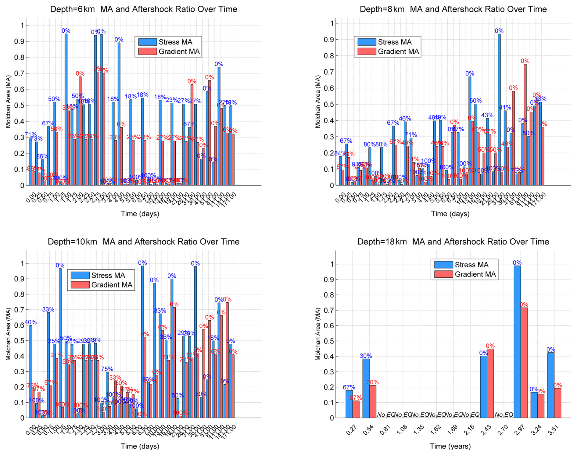
Figure 11 Molchan Area (MA) and aftershock ratio over time at depths of 6, 8, 10, and 18 km. Each subplot shows MA values derived from stress-based (blue bars) and stress-gradient-based (red bars) models, alongside the percentage of aftershocks located within high stress alert zones. Time labels on the x-axis represent post-mainshock intervals in days or years, depending on the depth. The presence of “No EQ” indicates intervals with no recorded aftershocks at that depth. This visualization compares the forecasting skill of stress-based versus gradient-based models across depth and time.

At shallow depths (6–8 km), the model achieves consistently strong performance, with numerous time intervals exhibiting MA values below 0.2 and aftershock capture ratios exceeding 50 %. These findings suggest that stress perturbations in the upper crust are more predictive and physically meaningful for aftershock nucleation. Notably, the stress-gradient model tends to produce lower MA values than the traditional stress-change model in these layers, indicating improved event prioritization. This supports the hypothesis that the spatial variation of stress – rather than its absolute amplitude – may play a more direct role in triggering aftershocks, particularly near rupture boundaries where instability gradients evolve dynamically.

In contrast, the model's performance becomes more variable at intermediate depths (e.g., 10 km), where MA values fluctuate widely despite moderate aftershock ratios. This behavior likely reflects the increased complexity and heterogeneity of stress transfer processes at mid-crustal levels, as well as potential limitations in model resolution or input constraints. At greater depths (≥ 18 km), the prevalence of time intervals without any recorded aftershocks (“No EQ” cases) suggests that post-seismic stress changes in the lower crust rarely lead to secondary ruptures – likely due to the re-stabilization of deep structures or intrinsic rheological resistance to stress perturbations. The AUC metric complements this analysis by quantifying the model's ability to rank stress (or gradient) values such that aftershock-prone locations consistently receive higher values than non-event locations. We observe a strong inverse correlation between MA and AUC: time intervals with low MA often correspond to high AUC scores (> 0.8), reinforcing both the spatial compactness and statistical reliability of our approach. While AUC excels in evaluating internal consistency and rank-based performance, MA provides an operational perspective – penalizing overly broad alarm zones and rewarding targeted spatial predictions.

Taken together, these two metrics offer a robust and interpretable framework for evaluating model performance across depths and time. Their joint application not only validates the physical plausibility of the stress-gradient model but also underscores its potential for operational integration into real-time aftershock hazard assessments, especially in shallow crustal zones where predictability is highest. In this evaluation, ΔCFF, dynamic ΔCFF(t), and ∇σ(t) are treated as continuous two-dimensional stress fields rather than discrete scalar predictors. Accordingly, their predictive performance is quantified using time-dependent AUC curves (Fig. 10) and Molchan diagrams (Fig. 11), which capture the full statistical evolution of the stress-triggering process. This curve-based representation avoids arbitrary discretization required by tabulated summary statistics and preserves the continuous nature of the underlying stress fields. The observed transitions in predictive skill – most notably the enhanced sensitivity of stress gradients at shallow depths during the early postseismic phase – are therefore interpreted directly from the dynamic evolution of these diagnostic curves.

3.4 Implications for Seismic Hazard Assessment

While the primary focus of this study is the modeling of multiscale stress evolution and gradient dynamics following large earthquakes, our findings have direct implications for enhancing probabilistic seismic hazard assessment (PSHA). Specifically, the derived stress gradient field (∇σ) offers a physically meaningful indicator of localized stress concentration and evolving instability potential in the crust – features that are often underrepresented in traditional PSHA models.

Current PSHA methodologies frequently employ smoothed seismicity approaches, which infer future hazard potential based on spatial interpolation of past earthquake occurrences (e.g., Mohamed et al., 2020; Elhadidy et al., 2021). These models offer valuable statistical insight but may lack direct ties to the underlying physical mechanisms of stress redistribution. Our approach provides a complementary, physics-based perspective by modeling how stress and its gradients evolve temporally and spatially after a major rupture. In doing so, it captures transient hazard escalation patterns that are difficult to detect using static seismicity patterns alone. Although our framework is not designed to replace traditional PSHA pipelines, it can enhance them by introducing depth-resolved stress indicators that reflect both mechanical and temporal properties of the crust. This is particularly relevant in tectonically complex regions – such as the active zones of the Red Sea, Taiwan, or the Dead Sea Rift – where stress transfer and cascading rupture dynamics play crucial roles in seismic hazard development (Al-Tarazi and Sandvol, 2022).

Future work may involve hybridizing our stress evolution model with smoothed seismicity or multicriteria PSHA frameworks to yield more responsive and mechanistically informed hazard maps. Such integration could refine spatial alert zones, inform early warning systems, and improve post-event risk communication by grounding hazard predictions in dynamic stress field behavior.

3.5 Sensitivity of α(t)–β(t) Parameters and Model Stability

To assess our time-dependent stress model's robustness and calibration sensitivity, we conducted a parametric sweep over initial values of the scaling factor β₀ while maintaining the $\mathit{\alpha }\left(t\right)=\mathrm{1}/(\mathrm{1}+t/\mathrm{49})$ decay profile constant. For each β₀ value, the model simulated stress fields and aftershock forecasts for the 2018 Hualien sequence. Performance was quantified using two complementary metrics: the Area Under the ROC Curve (AUC), which measures stress ranking skill, and the Molchan Area (MA), which assesses operational forecast efficiency. The results, summarized in Fig. 12, reveal a nonlinear relationship between β_o and predictive accuracy. AUC increases with β₀ up to ∼ 20, beyond which performance plateaus or slightly deteriorates.

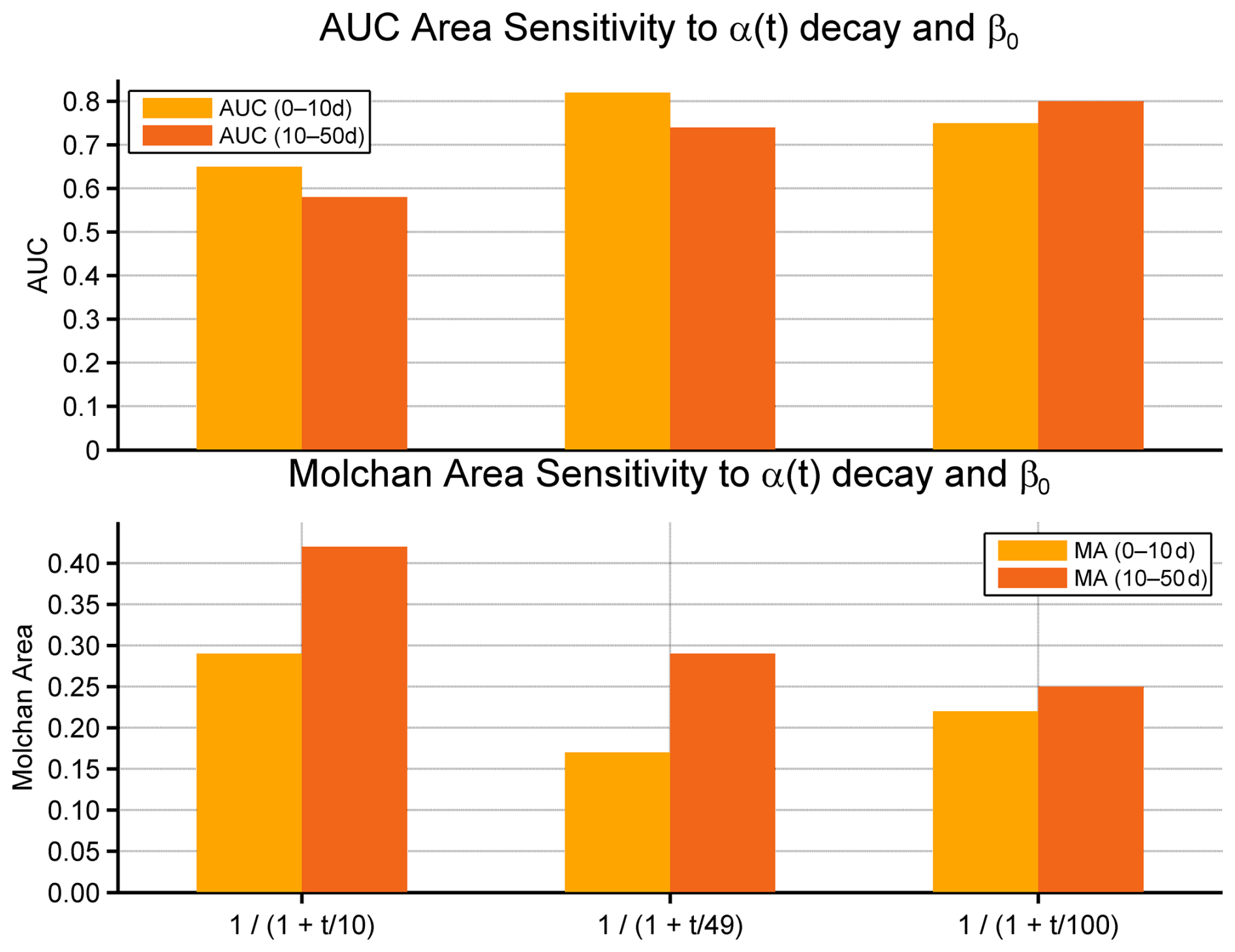
Figure 12 Variation in model performance as a function of the initial β₀ parameter. Panel (a) shows AUC, reflecting ranking accuracy; panel (b) shows Molchan Area (MA), quantifying spatial forecast efficiency. The results demonstrate the sensitivity of the DSGF model across different time windows and decay parameters.

Conversely, MA decreases initially, indicating improved efficiency, but begins rising again at high β₀ town-center values, suggesting spatial over-diffusion. This dual trend demonstrates the trade-off between ranking skill and spatial compactness. Notably, the optimal range for β₀ lies between 18 and 22, where AUC exceeds 0.84 and MA remains below 0.3. Values below 10 or above 30 result in unstable or inefficient forecasts. Moreover, the chosen value of β₀=20 aligns with theoretical constraints from the Banach fixed-point theorem and the Courant–Friedrichs–Lewy (CFL) condition, ensuring numerical stability and convergence of the iterative solution scheme.

4 Conclusions

This study presents a comprehensive and physically grounded framework that integrates Coulomb stress changes, stress gradients, and advanced mathematical modeling to improve the prediction of aftershock distributions. The proposed framework is designed as a physics-constrained stress evolution model rather than a parameter-fitting or machine-learning predictor. By coupling Rate-and-State friction laws, a KPP-type reaction–diffusion equation, and the Banach fixed-point theorem, we establish a novel numerical approach for modeling multiscale stress evolution following significant earthquakes. Central to the framework are the time-dependent parameters α(t) and β(t), which respectively govern stress memory decay and diffusion strength. Our theoretical and numerical analyses demonstrate how α influences the retention of historical stress and convergence rate, while β modulates the smoothing and reaction dynamics of the evolving stress field. The dynamic interaction between these parameters enables flexible control over the temporal and spatial behavior of stress evolution, enhancing both numerical stability and physical realism.

Conceptually, these internal diagnostics (STD/MSE) characterize the physical persistence of stress heterogeneity rather than direct seismic rates, with physical time implicitly governed through the reciprocal α(t)–β(t) coupling. This design avoids over-specifying poorly constrained deep-crustal temporal scales while maintaining a stable, physics-grounded stress-evolution framework. Temporal effects are explicitly incorporated only through the time-dependent memory parameter α(t) in the shallow crust, where Omori-type decay serves as a physically meaningful proxy for stress-memory loss. At greater depths, where seismicity is sparse and time scales are poorly constrained, iterations are interpreted as abstract relaxation steps, thereby avoiding uncertain deep-crustal time calibration while preserving the physical interpretability of the reaction–diffusion system. This distinction ensures that the model diagnostics remain grounded in the mechanics of stress evolution while acknowledging the complex, non-linear mapping between continuous stress fields and discrete seismic events.

Application of the model to the 2018 Hualien earthquake reveals a clear depth-dependent bifurcation in aftershock-driving mechanisms. During the initial 50 d post-mainshock, stress gradients outperform stress changes in predicting aftershock locations at shallow depths (6–10 km), due to their sensitivity to localized heterogeneity. Over longer timescales and at greater depths (≥ 18 km), stress changes become more predictive as stress gradients diminish with increased smoothing and reduced aftershock activity. This complementary relationship between stress metrics supports a dynamic, depth-aware modeling strategy. We further introduce the Molchan Area (MA) metric to evaluate operational forecasting skill, quantifying the trade-off between missed events and spatial coverage. The MA results reinforce our AUC-based findings, confirming that shallow crustal zones exhibit higher predictability and are especially suited for stress-gradient-based forecasting.

Beyond theoretical development, this study demonstrates the practical value of integrating physics-based models into seismic hazard mitigation. By linking multiscale stress dynamics with aftershock occurrence patterns, the framework provides timely, spatially explicit insights for post-earthquake risk assessment. This interdisciplinary contribution bridges geophysics, nonlinear modeling, and disaster science, offering a scalable and adaptable tool for real-world forecasting applications.

Appendix A

The following figures illustrate the relationship between stress changes, stress gradients, and the temporal distribution of aftershocks at different depths.

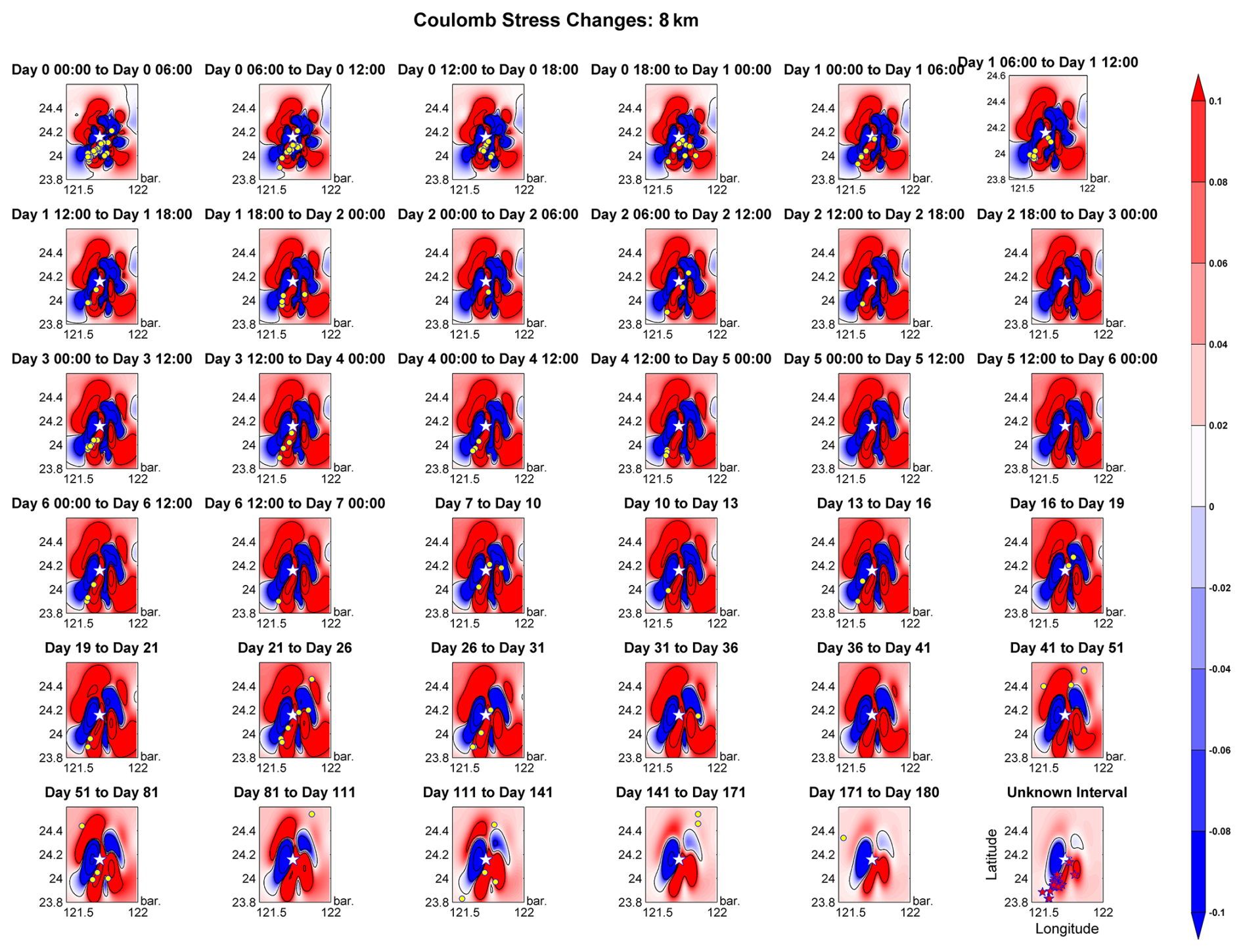
Figure A1 Temporal evolution of Coulomb stress changes at a depth of 8 km during the first 180 d following the 2018 Hualien earthquake (M_w 6.4). Each panel represents the Coulomb stress changes distribution over specific time intervals, with red regions indicating positive stress changes (stress loading) and blue regions indicating negative stress changes (stress unloading). The contours highlight the areas (> 0.1 bar) of significant stress concentration. The yellow circles indicate the epicenters of aftershocks occurring within 180 d of the mainshock, while the red stars in the final panel represent those occurring 2 to 3 years after the mainshock.

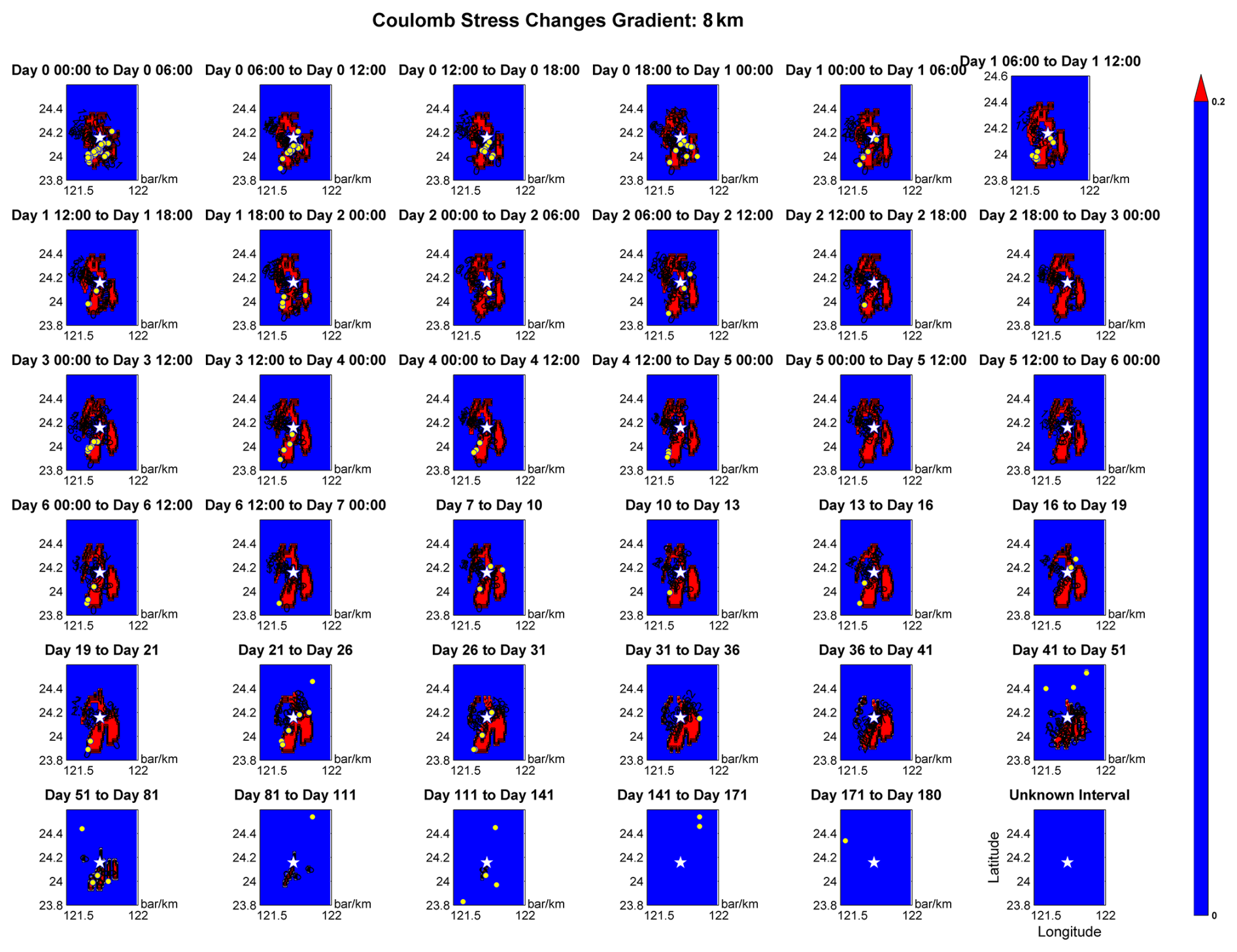
Figure A2 Temporal evolution of Coulomb stress changes gradients at a depth of 8 km during the first 180 d following the 2018 Hualien earthquake (M_w 6.4). Each panel illustrates the distribution of stress gradients (in bar km⁻¹) over specific time intervals. Regions with high stress gradients (> 0.2 bar km⁻¹) are marked in red, while blue areas represent negligible gradients.

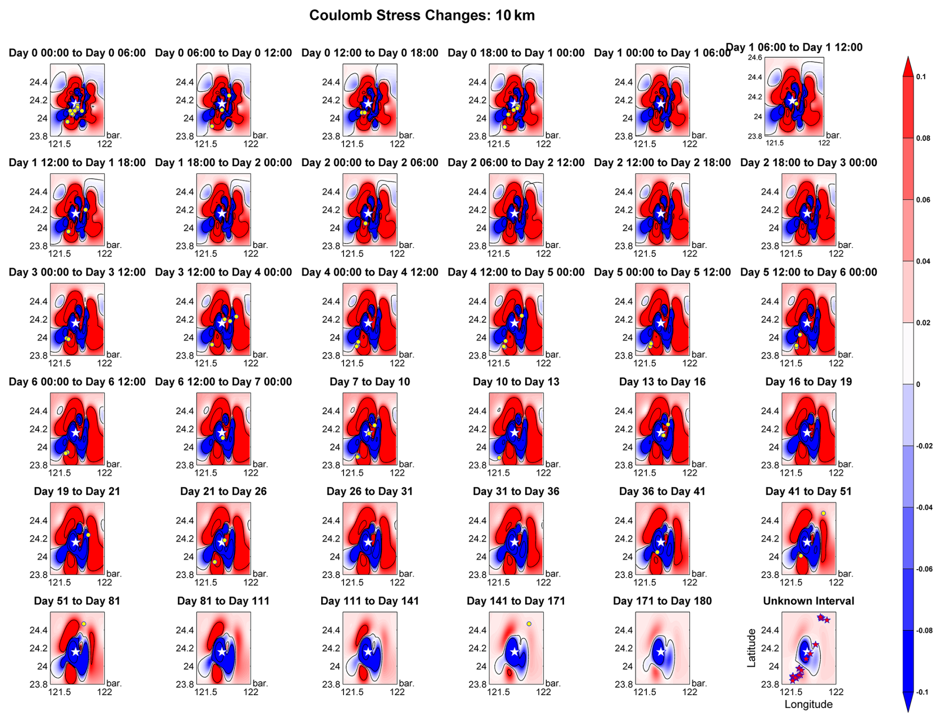
Figure A3 Temporal evolution of Coulomb stress changes at a depth of 10 km during the first 180 d following the 2018 Hualien earthquake (M_w 6.4). Each panel represents the Coulomb stress changes distribution over specific time intervals, with red regions indicating positive stress changes (stress loading) and blue regions indicating negative stress changes (stress unloading). The contours highlight the areas (> 0.1 bar) of significant stress concentration. The yellow circles indicate the epicenters of aftershocks occurring within 180 d of the mainshock, while the red stars in the final panel represent those occurring 2 to 3 years after the mainshock.

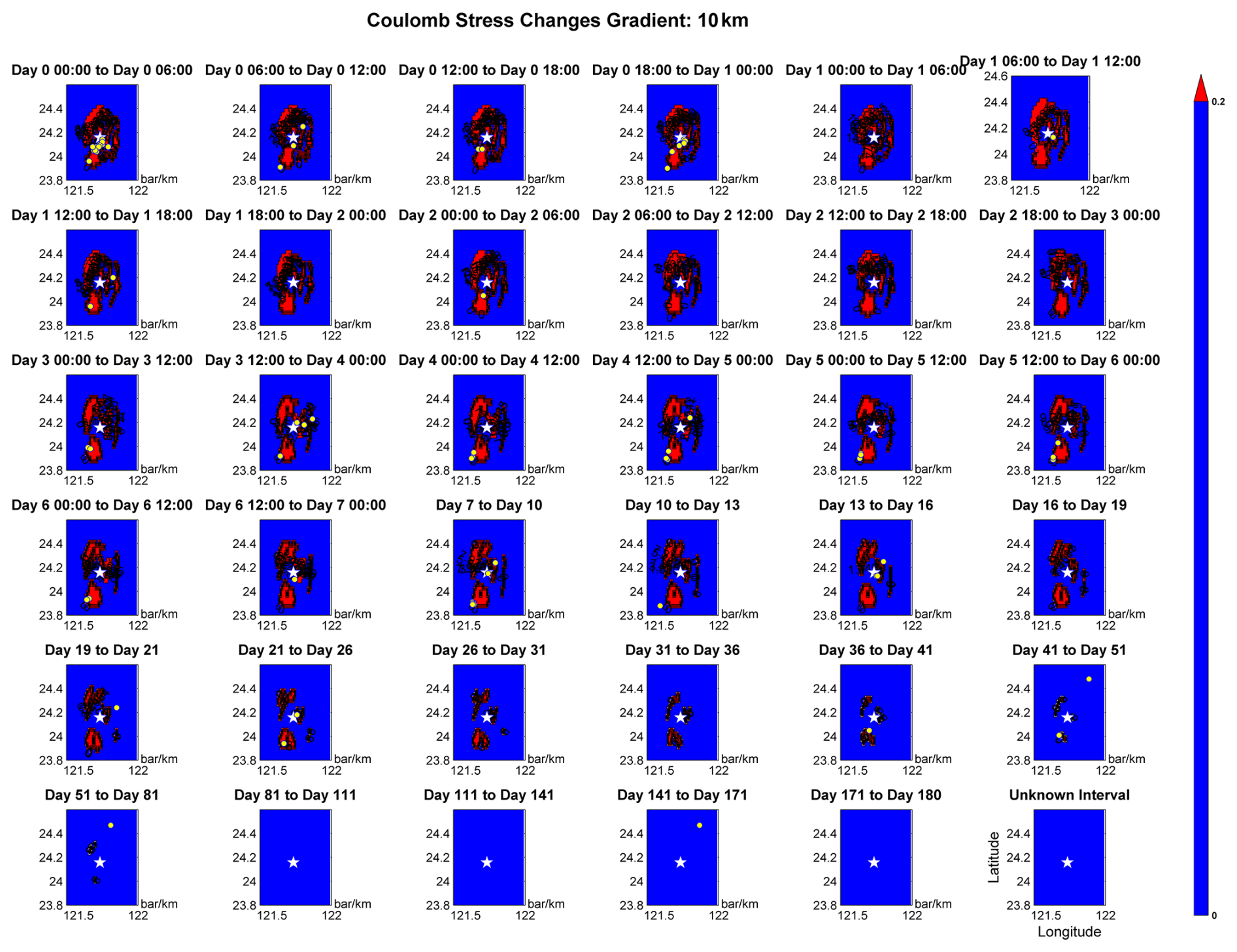
Figure A4 Temporal evolution of Coulomb stress changes gradients at a depth of 10 km during the first 180 d following the 2018 Hualien earthquake (M_w 6.4). Each panel illustrates the distribution of stress gradients (in bar km⁻¹) over specific time intervals. Regions with high stress gradients (> 0.2 bar km⁻¹) are marked in red, while blue areas represent negligible gradients.

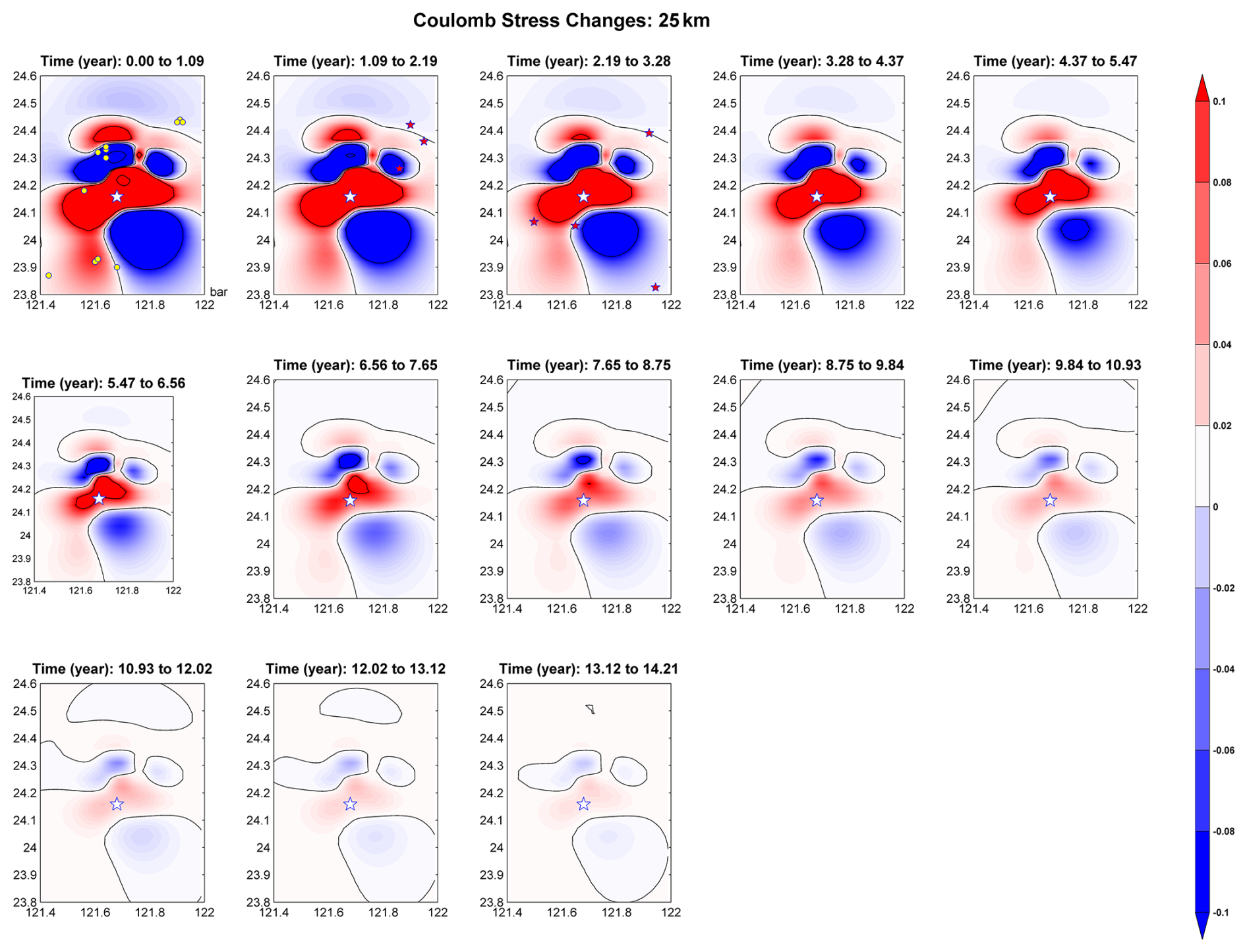
Figure A5 This figure depicts the evolution of Coulomb stress changes at a depth of 25 km over a period exceeding 14 years following the mainshock. The color scale highlights regions of increased stress (red) and decreased stress (blue). The yellow circles mark aftershock epicenters within the first 180 d post-mainshock, while red stars denote aftershocks occurring 2 to 3 years later. The observed stress redistribution patterns reveal a gradual decay in stress concentration over time, reflecting stress diffusion and the diminishing influence of the initial stress perturbation. Compared to shallower depths, the stress field at 25 km remains more uniform, with fewer high-stress regions correlating with aftershock activity. As time progresses, stress changes stabilize, reducing their association with aftershock distributions, particularly in the later years.

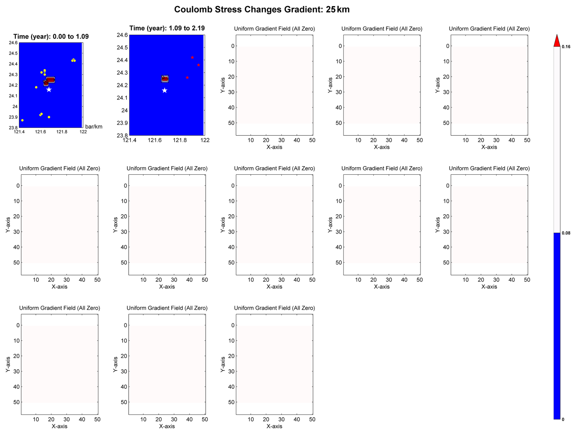
Figure A6 This figure illustrates the Coulomb stress change gradients at a depth of 25 km over time. The first two panels display the stress gradient distribution within the initial 2.19 years following the mainshock. Yellow circles represent aftershock epicenters within 180 d, and red stars indicate those occurring 2 to 3 years post-mainshock. Subsequent panels show uniform gradient fields where stress gradients approach zero, reflecting minimal heterogeneity in the stress field. This indicates that, at this depth, diffusion and reaction processes have homogenized the stress gradients, reducing their predictive capability for aftershock locations as time progresses. The absence of significant stress gradient changes in later panels highlights the stabilization of the stress field.