Improving dynamical climate predictions with machine learning: insights from a twin experiment framework

Systematic errors in dynamical climate models remain a significant challenge to accurate climate predictions, particularly when modeling the nonlinear coupling between the atmosphere and ocean. Despite notable advances in dynamical climate modeling that have improved our understanding of climate variability, these systematic errors can still degrade prediction skills. In this study, we adopt a twin experiment framework with a reduced-order coupled atmosphere-ocean model to explore the utility of machine learning in mitigating these errors. Specifically, we train a data-driven model on data assimilation increments to learn and emulate the underlying dynamical climate model error, which is then integrated with the dynamical climate model to form a hybrid model. Comparison experiments show that the hybrid model consistently outperforms the standalone dynamical climate model in predicting atmospheric and oceanic variables. Further investigation using hybrid models that correct only atmospheric or only oceanic errors reveals that atmospheric corrections are essential for improving short-term predictions, while concurrently addressing both atmospheric and oceanic errors yields superior performance in long-term climate prediction.

1 Introduction

Climate prediction aims at predicting the future state of the climate system based on the initial conditions and external forcings (e.g., greenhouse gases and aerosols) covering various lead times from seasons to decades (Merryfield et al., 2020). It helps scientists, policymakers, and communities in understanding potential risks and impacts. It differs from climate projections that focus primarily on capturing long-term climate trends and patterns from several decades to centuries by anticipating changes in external forcings and their impact on the climate system.

Dynamical climate models, such as atmosphere-ocean coupled general circulation models, have been widely used for climate predictions (e.g., Doblas-Reyes et al., 2013b; Boer et al., 2016). Uncertainties in initial conditions fed to dynamical climate models and model errors are two critical sources that limit the prediction skill of dynamical climate models. To reduce the uncertainties of initial conditions, climate prediction centers (Balmaseda and Anderson, 2009; Doblas-Reyes et al., 2013a) have been evolving towards the use of data assimilation  (DA, Carrassi et al., 2018) which combines observations with the dynamical climate models to estimate the best initial conditions of the climate prediction (Penny and Hamill, 2017). Model errors can arise from a variety of sources, including model parameterizations (Palmer, 2001), unresolved physical processes (Moufouma-Okia and Jones, 2015), and numerical approximations (Williamson et al., 1992). Despite substantial efforts to improve dynamical climate models, these errors remain notably large (e.g., Richter, 2015; Palmer and Stevens, 2019; Richter and Tokinaga, 2020; Tian and Dong, 2020).

There is a growing interest in utilizing machine learning (ML) techniques to address errors in a dynamical climate model. ML can be employed to construct a data-driven predictor of model errors, which can then be integrated with the dynamical climate model to create a hybrid statistical-dynamical model (e.g., Watson, 2019; Farchi et al., 2021a; Brajard et al., 2021; Watt-Meyer et al., 2021; Bretherton et al., 2022; Chen et al., 2022; Gregory et al., 2024).

Some notable studies (e.g., Watson, 2019; Brajard et al., 2021; Farchi et al., 2021a, 2023) focused on methodological developments within low-order or simplified coupled models operating in an idealized framework where the ground truth is known. For example, Farchi et al. (2021a) investigated two approaches in a two-scale Lorenz model, both of which are potential candidates for implementation in operational systems. One approach involves correcting the so-called resolvent of the dynamical climate model (i.e., modifying the model output after each numerical integration of the model). The other approach entails adjusting the ordinary or partial differential equation governing the model tendency before the numerical integration of the model. Similarly, Watson (2019) examined the tendency correction approach in the Lorenz 96 model. Brajard et al. (2021) explored the resolvent correction approach in the two-scale Lorenz model as well as in a low-order coupled atmosphere-ocean model called the Modular Arbitrary-Order Ocean-Atmosphere Model (MAOOAM, De Cruz et al., 2016). Their study aimed to infer the model errors associated with unresolved processes within the dynamical climate model. While Brajard et al. (2021) conducted prediction experiments using perfect initial conditions, more recent studies such as Farchi et al. (2023) examined the performance of hybrid models initialized with imperfect conditions, using a two-layer quasi-geostrophic (QG) model. Despite recent efforts to incorporate more realistic settings, hybrid models are still frequently evaluated under idealized conditions in which the initial state, taken from the same model as the reference, is assumed to be perfectly known.

Several other investigations tested ML-based error correction methods in realistic numerical weather prediction (NWP) (e.g., Bonavita and Laloyaux, 2020; Watt-Meyer et al., 2021; Bretherton et al., 2022; Chen et al., 2022; Gregory et al., 2024; Farchi et al., 2025). Bonavita and Laloyaux (2020) demonstrated that ML can emulate model error corrections derived from weak-constraint 4D-Var in ECMWF's Integrated Forecasting System (IFS), highlighting the potential of ML to systematically reduce model errors throughout the atmospheric column. Watt-Meyer et al. (2021) used random forests trained on FV3GFS nudging tendencies to correct model tendencies, achieving stable year-long runs and improved short-term forecasts for 500 hPa height, surface pressure, and near-surface temperature. Bretherton et al. (2022) corrected coarse-grid model errors by applying ML-learned temperature and humidity tendencies from a high-resolution reference, significantly improving prediction skills and precipitation patterns. Chen et al. (2022) used ML to learn the analysis increments (i.e., the differences between the analysis and background, Evensen, 2003) and correct state-dependent model errors in NOAA's FV3-GFS. The online application of these corrections during model integration led to enhanced DA performance and improved 10 d predictions. Gregory et al. (2024) developed a hybrid dynamical–statistical framework that employs convolutional neural networks trained on sea ice concentration (SIC) assimilation increments, leading to improved five-year sea ice simulations. Most recently, Farchi et al. (2025) implemented an ML-based model error correction scheme within ECMWF's operational IFS. Their results indicated that offline-trained networks can already offer robust corrections, while online updates further enhance adaptability under diverse conditions. However, the potential benefits of ML-based model error correction for climate prediction across different time scales remain largely unexplored. This is primarily due to the sparsity of long-term observational records (such as those spanning the 20th century) in both time and space, which presents significant challenges for developing effective ML-based error correction models for climate prediction applications.

In this study, we investigate the potential of ML-based model error correction for climate prediction within an idealized framework. To this end, we adopt the hybrid modeling approach introduced by Brajard et al. (2021), which is based on MAOOAM. The ML-based error correction model aims to learn and correct dynamical climate model errors using analysis increments. Unlike Brajard et al. (2021), we conduct ensemble predictions with imperfect initial conditions (Farchi et al., 2023), which better reflect realistic prediction scenarios (Wang et al., 2019; Bethke et al., 2021). Specifically, we examine how the effectiveness of ML-based error correction varies across different climate time scales. Moreover, given that the respective roles of atmospheric and oceanic errors in limiting climate predictability are not fully understood, we assess the relative contributions of these components to the overall prediction error.

The article is organized as follows: Sect. 2 introduces the main methodological aspects of the study. Section 3 shows the prediction skill of the hybrid model compared with the dynamical climate model and discusses factors affecting the prediction skill of the hybrid model. Finally, a brief concluding summary is presented in Sect. 4.

2 Methodology

In this study, we restrict our scope to model errors stemming solely from coarse resolutions in the atmospheric component. In this section, we describe the model (Sect. 2.1), DA technique (Sect. 2.2), and the ML approach (Sect. 2.3). Rather than focusing on methodological developments, our goal is to examine how the advantages of ML-based error correction evolve in time in the context of climate prediction and to determine which errors should be corrected at different timescales. Further details in experiments are provided in Sect. 2.4.

2.1 Modular arbitrary-order ocean-atmosphere model

We utilize MAOOAM developed by De Cruz et al. (2016) in our study. MAOOAM consists of a two-layer QG atmospheric component coupled with a QG shallow-water oceanic component. The coupling between these components incorporates wind forcings, radiative and heat exchanges, enabling it to simulate climate variability. MAOOAM has been widely employed in qualitative analyses for various purposes (e.g., Penny et al., 2019; Brajard et al., 2021). Moreover, MAOOAM's numerical efficiency allows us to execute numerous climate prediction experiments at a relatively low computational cost.

In MAOOAM, the model variables are represented in terms of spectral modes. Specifically, d_ax (d_ox) represents the x-direction resolution, and d_ay (d_oy) represents the y-direction resolution in the atmosphere (ocean). The model state comprises n_a ($n_{\mathrm{a}}=d_{\mathrm{a}y}(\mathrm{2}{d}_{\mathrm{a}x}+\mathrm{1})$) modes of the atmospheric streamfunction ψ_a and temperature anomaly θ_a, as well as n_o (n_o=d_oyd_ox) modes of the oceanic streamfunction ψ_o and temperature anomaly θ_o. Consequently, the model state can be expressed as:

$$\begin{array}{}\text{(1)}& \begin{array}{rl}\mathit{x}=& ({\mathit{\psi }}_{\mathrm{a},\mathrm{1}},{\mathit{\psi }}_{\mathrm{a},\mathrm{2}},\mathrm{\dots },{\mathit{\psi }}_{\mathrm{a},n_{\mathrm{a}}},{\mathit{\theta }}_{\mathrm{a},\mathrm{1}},{\mathit{\theta }}_{\mathrm{a},\mathrm{2}},\mathrm{\dots },{\mathit{\theta }}_{\mathrm{a},n_{\mathrm{a}}},\\ & {\mathit{\psi }}_{\mathrm{o},\mathrm{1}},{\mathit{\psi }}_{\mathrm{o},\mathrm{2}},\mathrm{\dots },{\mathit{\psi }}_{\mathrm{o},n_{\mathrm{o}}},{\mathit{\theta }}_{\mathrm{o},\mathrm{1}},{\mathit{\theta }}_{\mathrm{o},\mathrm{2}},\mathrm{\dots },{\mathit{\theta }}_{\mathrm{o},n_{\mathrm{o}}})\end{array}\end{array}$$

The total number of variables in the model state is 2n_a + 2n_o. Note that n_a is typically larger than n_o, reflecting the distinct characteristics of the two components in MAOOAM. The atmosphere exhibits faster dynamics and smaller-scale variability, necessitating a greater number of modes to adequately capture its behavior. In contrast, the ocean evolves more slowly and is dominated by larger-scale processes, which can be effectively represented using fewer modes (De Cruz et al., 2016). It is also important to note that variables with lower indices correspond to low-order (large-scale) processes, while variables with higher indices correspond to high-order (small-scale) processes. Like many other models formulated in spectral space, MAOOAM offers flexibility in adjusting the number of atmospheric and oceanic variables by simply modifying the model resolution in spectral space.

In this study, we utilize two different configurations of MAOOAM: one denoted as M56 and the other as M36. The M56 configuration comprises a total of 56 variables, with 20 atmospheric modes (n_a=20) and 8 oceanic modes (n_o=8). Specifically, the atmosphere in M56 operates at a 2x−4y (i.e., d_ax=2 and d_ay=4) resolution, and the ocean operates at a 2x−4y (i.e., d_ox=2 and d_oy=4) resolution. On the other hand, the M36 configuration includes 36 variables, with 10 atmospheric modes (n_a=10) and 8 oceanic modes (n_o=8), identical to M56. The atmospheric component in M36 operates at a 2x−2y resolution (d_ax=2, d_ay=2), while the ocean component matches that of M56. Figure 1 displays time series of three key variables in the true model M56 and the dynamical climate model M36 in spectral space, illustrating their different evolution patterns (De Cruz et al., 2016).

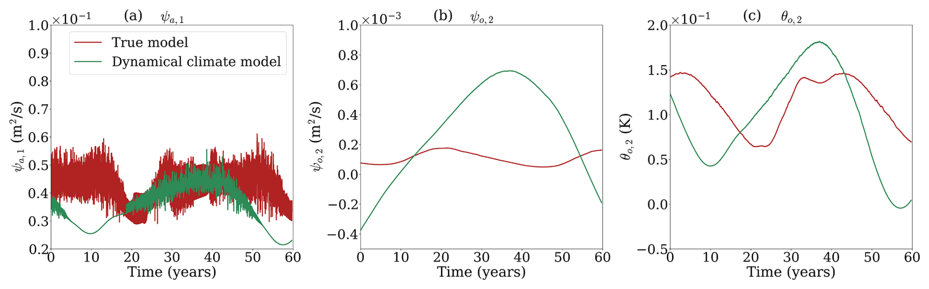
Figure 1 Time series of the true model (red lines) and the dynamical climate model (green lines) for three key variables: (a) ψ_a,1, (b) ψ_o,2, and (c) θ_o,2.

It is important to note that the key distinction between M36 and M56 lies in the atmosphere, where M36 has a reduced number of atmospheric modes, specifically 10 modes fewer than M56 in the y-direction. This difference leads to a lack of higher-order atmospheric modes in M36, thereby unable to capture small-scale variability. The atmospheric error in the y-direction propagates to the atmosphere in the x-direction and the ocean component through the coupling terms in the equations. Consequently, the primary source of model error in this study is attributed to the coarse resolution of the atmospheric component in the y-direction.

2.2 Ensemble Kalman filter

The Ensemble Kalman Filter (EnKF) is a flow-dependent and multivariate DA method and has been implemented for climate prediction (e.g., Zhang et al., 2007; Karspeck et al., 2013; Wang et al., 2019). The EnKF constructs the background error covariance from the dynamical ensemble. The utilization of an ensemble-based error covariance ensures that the assimilation updates approximately respect to the model dynamics, thereby mitigating assimilation shocks (Evensen, 2003).

All experiments in this study are conducted using the DAPPER package (Raanes, 2018). The overall experimental setup is described in Sect. 2.4 and depicted in Fig. 2. Specifically, we employ the finite-size ensemble Kalman filter (EnKF-N) method proposed by Bocquet et al. (2015). This method adaptively adjusts the inflation factor, thereby reducing the need for extensive manual tuning and enhancing the performance of the assimilation experiments. It is worth mentioning that we expect no significant alterations in the conclusions of this paper when using the traditional EnKF methods instead of EnKF-N.

Figure 2 Schematic of experiments.

2.3 Artificial neural network architecture

We consider the dynamical climate model (described in Sect. 2.1) in the following form:

$$\begin{array}{}\text{(2)}& {\mathit{x}}_{k+\mathrm{1}}=\mathcal{M}\left({\mathit{x}}_k\right),\end{array}$$

where x_k+1 represents the full model state at t_k+1, x_k represents the full model state at t_k and ℳ represents the dynamical climate model integration from time t_k to t_k+1. The model error at time t_k+1 is defined as:

$$\begin{array}{}\text{(3)}& {\mathit{\epsilon }}_{k+\mathrm{1}}={\mathit{x}}_{k+\mathrm{1}}^{\mathrm{t}}-{\mathit{x}}_{k+\mathrm{1}},\end{array}$$

where ${\mathit{x}}_{k+\mathrm{1}}^{\mathrm{t}}$ represents the true state at time t_k+1.

We aim to use ANN to emulate the model error ε_k+1. Since the truth is not known in practice, the training of ANN uses the analysis increments produced by the EnKF (Brajard et al., 2021; Farchi et al., 2021b; Gregory et al., 2024). The architecture of ANN used in this study consists of four layers:

• The input layer includes a batch normalization layer (Ioffe, 2017), which helps to regularize and normalize the training process.

• The second layer is a dense layer with 100 neurons. It applies the rectified linear unit (ReLU) activation function, which introduces non-linearity into the network.

• The third layer has the same configuration as the second layer, with 50 neurons and ReLU activation function.

• The output layer, which is a dense layer with a linear activation function and produces the final predictions, is optimized using the “RMSprop” optimizer (Hinton et al., 2012) and includes an L2 regularization term with a value of 10⁻⁴.

During training, the ANN model is trained with a batch size of 128 and for a total of 300 epochs.

The error surrogate model can be expressed as follows:

$$\begin{array}{}\text{(4)}& {\mathit{\epsilon }}_{k+\mathrm{1}}^{\prime }={\mathcal{M}}_{\mathrm{ANN}}\left({\mathit{x}}_k\right),\end{array}$$

where ℳ_ANN represents the data-driven model built by ANN and ${\mathit{\epsilon }}_{k+\mathrm{1}}^{\prime }$ represents the model error estimated by ANN. The full state at time t_k+1 of the hybrid model can be expressed as follows:

$$\begin{array}{}\text{(5)}& {\mathit{x}}_{k+\mathrm{1}}^{\mathrm{h}}=\mathcal{M}\left({\mathit{x}}_k\right)+{\mathcal{M}}_{\mathrm{ANN}}\left({\mathit{x}}_k\right)\end{array}$$

2.4 Experiment settings

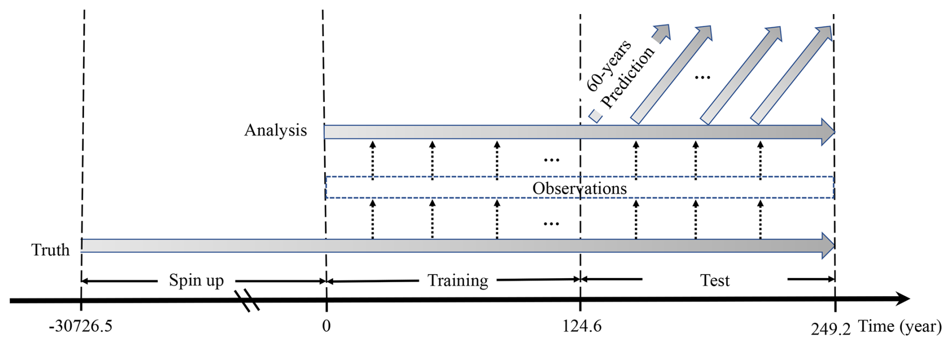
We present the experimental setup in Fig. 2. The experiments are conducted using two configurations of MAOOAM, as described in Sect. 2.1. The configuration with 56 variables (M56, Sect. 2.1) represents the true climate system, while the configuration with 36 variables (M36, Sect. 2.1) represents a dynamical climate prediction system. The experiments depicted in Fig. 2 are performed as follows:

• We integrate the M56 configuration with a time step of approximately 1.6 min for a spin-up period of 30 726.5 years, as specified in De Cruz et al. (2016). Following the spin-up period, we continue the simulation for an additional 249 years, which we refer to as the “truth”. To generate observations, we perturb the “truth” state using a Gaussian random noise. The standard deviation (σ^hf) of the noise is set to 10 % of the temporal standard deviation of the true state (x^t) after subtracting the one-month running average. Observations are generated every 27 h in spectral space, while the observation operator H is the identity operator (H=I) and is also applied in spectral space.

• We assimilate synthetic observations into the dynamical climate model (M36) and generate analysis with 50 ensemble members over the same period as the truth. The initial conditions of the ensemble are randomly sampled from a long free-run simulation of M36 after the spin-up period.

• We generate several sets of ensemble predictions with the dynamical climate model (M36) or the hybrid model. The prediction experiments start in each second year from the year 125 to the year 185, with each prediction lasting for 60 years. Each prediction consists of 50 ensemble members. The initial conditions for these ensembles are taken from the analysis (Fig. 2).

Note that both the observations and DA are conducted in the spectral space. Accordingly, the hybrid model is developed within the spectral space.

We split the analysis into two parts:

• Training data: The former 124.6 years of the dataset are used to train the ANN parameters to build the hybrid model (Fig. 2).

• Test data: The latter 124.6 years of the dataset are used to initialize prediction experiments (Fig. 2).

It is worth noting that since we employ the same ANN configurations as outlined in Brajard et al. (2021), the ANN parameters in this study are trained only once, without any modifications throughout the training process by using a separate validation set. We examined the loss curves (not shown in this study) to assess the training behavior. The loss curves provided evidence that the network was continuing to learn without signs of overfitting throughout the training process.

Brajard et al. (2021) focused on developing the hybrid model methodology; our study aims to explore the evolution of prediction skill as a function of lead time. We assess the prediction skill over a wider range of lead times, specifically up to 50 d for atmospheric variables and up to 60 years for oceanic variables. By examining the skill at various lead times, we can gain insights into the temporal evolution and long-term performance of the hybrid model, providing a more comprehensive understanding of its capabilities and limitations. To do so, our experimental setup is different from that of Brajard et al. (2021) in the following ways:

• We extended the simulation time to 219.2 years, while Brajard et al. (2021) generated an analysis dataset spanning 62 years for training, validation and testing. We divided our analysis dataset into two distinct parts: one for training the ANN and the other for testing purposes. This separation allows us to independently evaluate the performance of the trained ANN using data that was not used during the training phase.

• Our experiments utilize the analysis as initial conditions, while Brajard et al. (2021) uses perfect initial conditions (i.e., the truth) to initialize predictions. This choice reflects a more realistic scenario, as perfect knowledge of initial conditions is rarely available in the real framework. By using the analysis as initial conditions, we aim to capture the practical challenges associated with imperfect knowledge of the initial state in climate prediction.

• Our study incorporates an ensemble prediction strategy with 50 members, while Brajard et al. (2021) performed predictions using a single member (i.e., deterministic prediction). In the climate prediction community, probabilistic predictions based on ensembles are widely recognized. Ensembles provide a valuable means of quantifying uncertainty in climate predictions by generating multiple realizations rather than a single deterministic prediction.

2.5 Validation metrics

To evaluate the prediction skill of each variable, we employ the correlation and root mean square error (RMSE) skill score (RMSE-SS), which are commonly used metrics in weather forecasting and climate prediction. The correlation is defined as:

$$\begin{array}{}\text{(6)}& \text{Correlation}={\displaystyle \frac{\sum _{i=\mathrm{1}}^N(x_i-\stackrel{\mathrm{‾}}{x})(y_i-\stackrel{\mathrm{‾}}{y})}{\sqrt{\sum _{i=\mathrm{1}}^N(x_i-\stackrel{\mathrm{‾}}{x}{)}^{\mathrm{2}}\sum _{i=\mathrm{1}}^N(y_i-\stackrel{\mathrm{‾}}{y}{)}^{\mathrm{2}}}}},\end{array}$$

where x represents the prediction (ensemble mean) and y represents the truth. N is the total number of prediction experiments and is equal to 30 (Sect. 2.4).

The RMSE is calculated as follows:

$$\begin{array}{}\text{(7)}& \text{RMSE}=\sqrt{{\displaystyle \frac{\mathrm{1}}{N}}\sum _{i=\mathrm{1}}^N(x_i-y_i{)}^{\mathrm{2}}},\end{array}$$

where x represents the prediction (ensemble mean), y represents the truth, and N is the total number of prediction experiments. The RMSE-SS compares the RMSE of the prediction to the RMSE of a persistence prediction. It is defined as:

$$\begin{array}{}\text{(8)}& \text{RMSE-SS}=\mathrm{1}-{\displaystyle \frac{{\mathrm{RMSE}}_{\mathrm{prediction}}}{{\mathrm{RMSE}}_{\mathrm{persistence}}}},\end{array}$$

where RMSE_prediction represents the RMSE between the prediction (ensemble mean) and the truth and RMSE_persistence represents the RMSE between a persistence prediction (where the state remains the same as the initial conditions) and the truth. A positive RMSE-SS indicates that the prediction outperforms persistence and demonstrates skill. On the other hand, a negative RMSE-SS indicates that the prediction performs worse than the persistence and lacks skill. By utilizing the correlation and RMSE-SS, we can assess and compare the skill of the predictions generated by the dynamical climate model and the hybrid model across different variables within the same panel, as shown in Fig. 4.

To assess the statistical significance of the correlation and RMSE-SS, we perform a two-tailed Student's t-test based on the p-value. For the correlation, the null hypothesis is that the correlation is not significantly different from zero, implying no relationship between the predictions and truth. For RMSE-SS, we perform a hypothesis test to determine whether the squared errors (SE) from the prediction and persistence methods differ significantly. Specifically, we compute the SE for both methods and apply a two-tailed t-test to assess whether their means are significantly different. Assuming sufficiently large sample sizes, the difference between the mean squared error (MSE) can be approximated as normally distributed. This approximation is valid under the conditions that the SE from the two methods are independent and have the same mean value:

$$\begin{array}{rl}& {\text{MSE}}_{\text{prediction}}-{\text{MSE}}_{\text{persistence}}\\ & \sim \mathcal{N}\left(\mathrm{0},{\displaystyle \frac{s_{\text{prediction}}^{\mathrm{2}}}{N}}+{\displaystyle \frac{s_{\text{persistence}}^{\mathrm{2}}}{N}}\right),\end{array}$$

where $s_{\text{prediction}}^{\mathrm{2}}$ and $s_{\text{persistence}}^{\mathrm{2}}$ are the sample variances of the SE, and N is the total number of prediction experiments. The resulting p-value represents the probability of observing the given difference (or larger) under the null hypothesis. A p-value below 0.05 is considered statistically significant, indicating that the prediction and persistence methods exhibit meaningfully different error characteristics.

To estimate the uncertainties of correlation and RMSE-SS, we utilize the bootstrap method. We randomly select, with replacement, 30 data points from the 30 prediction experiments and calculate the correlation and RMSE-SS based on this sampled data. This procedure is repeated 10 000 times, resulting in a sample of 10 000 correlation and RMSE-SS values. The standard deviation of this sample is then used to estimate the uncertainties associated with the correlation and RMSE-SS. By conducting the t-test and utilizing the bootstrap method, we can obtain a more comprehensive understanding of the significance and reliability of the correlation and RMSE-SS values obtained from the prediction experiments.

In climate prediction, time-mean quantities such as monthly (Wang et al., 2019) or annual averages (Boer et al., 2016; Bethke et al., 2021) are often used because time averaging reduces the impact of chaotic weather variability, making the underlying climate signals more apparent. They also better meet the practical needs of sectors such as agriculture and energy, where planning is often based on mean conditions. In contrast, predicting higher-order statistics accurately remains challenging due to model limitations and computational costs, particularly when high-resolution Earth system models are required. Nevertheless, there is growing interest in representing complex statistical properties to improve the prediction of extreme events and support climate risk assessments.

To evaluate prediction skill across different time scales, we apply two complementary strategies. For short-term predictions, instantaneous outputs sampled every 27 h are used to represent daily variations. For long-term predictions, model outputs are averaged annually to assess the ability to capture low-frequency variability.

3 Results

3.1 Prediction skill

The distinction between short-term (daily) and long-term (yearly-averaged) prediction scales in this study is based on the fundamentally different error growth characteristics of atmospheric and oceanic variables. As illustrated in Fig. 3, atmospheric variables exhibit rapid error amplification, with a doubling error time of approximately one day and saturation occurring within about ten days. In contrast, oceanic variables demonstrate much slower error growth, with errors roughly doubling over the first year and continuing to grow gradually over the subsequent decade.

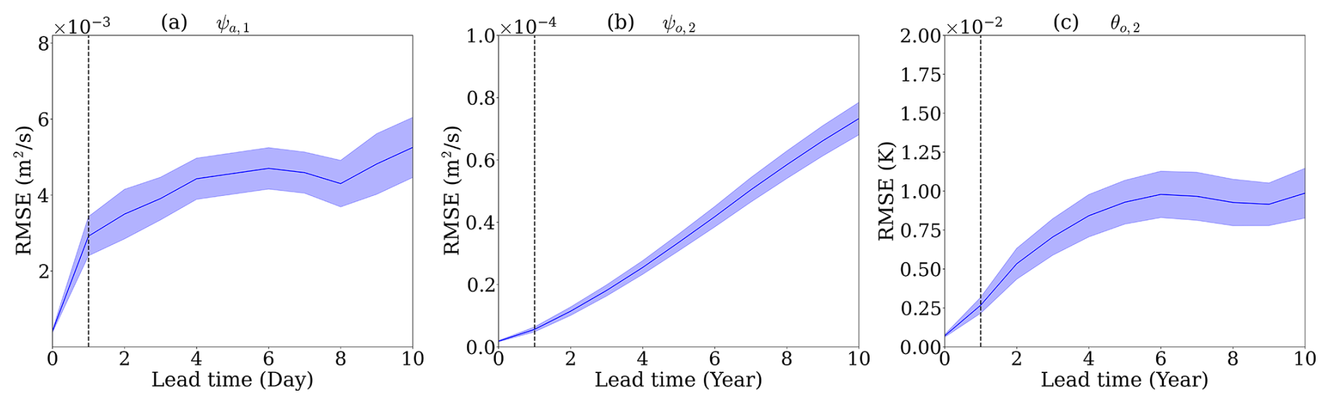
Figure 3 RMSE of dynamical prediction as a function of lead time for three key variables in spectral space: (a) ψ_a,1, (b) ψ_o,2, and (c) θ_o,2. The atmospheric variable (ψ_a,1) is evaluated based on instantaneous outputs sampled every 27 h, while the oceanic variables (ψ_o,2 and θ_o,2) are evaluated using yearly averages. Shading indicates one standard deviation, representing the uncertainty of prediction skill, estimated using the bootstrap method. The vertical dashed lines represent the time of doubling error.

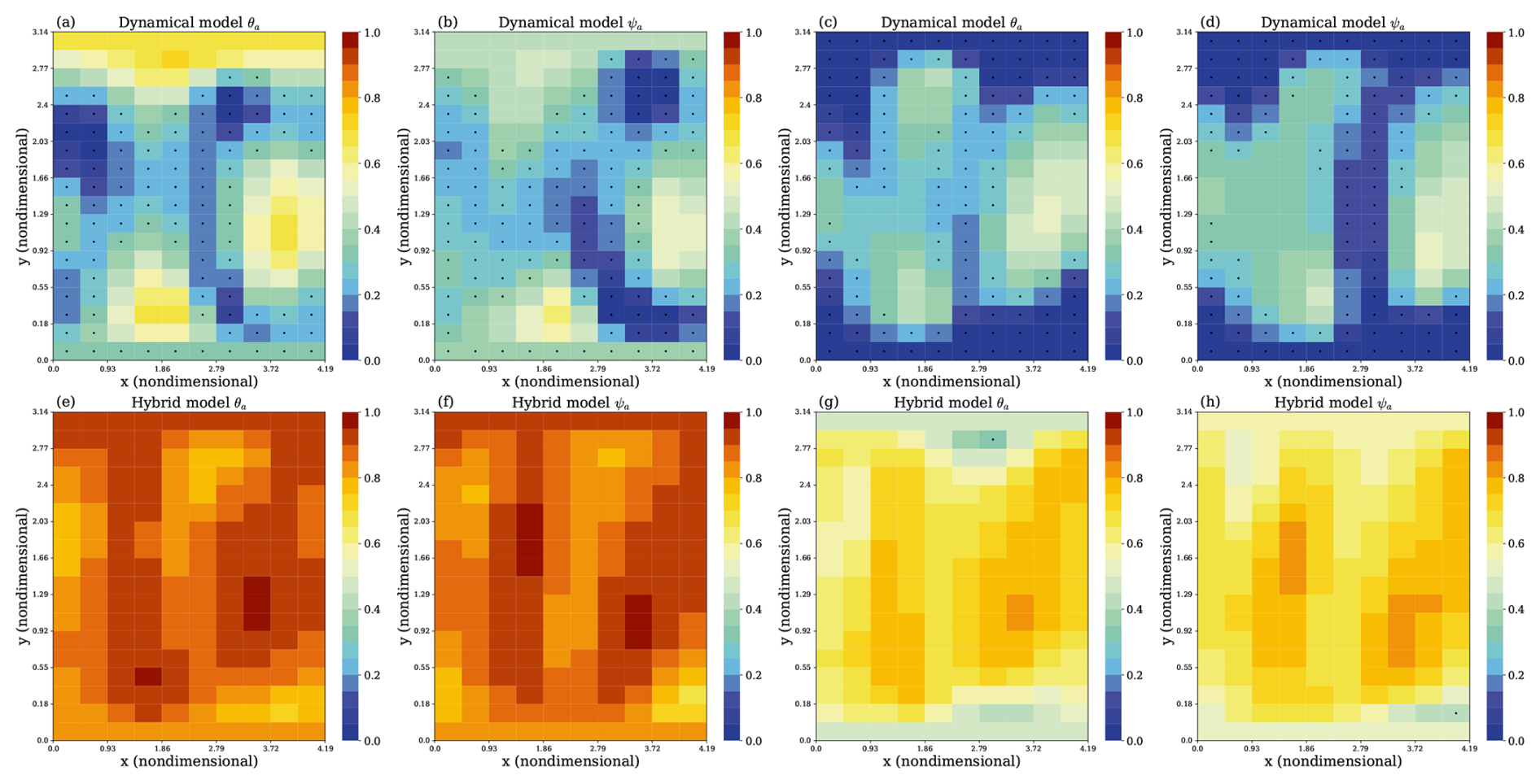
Figure 4 Correlation and RMSE-SS as a function of the prediction lead time for different variables. (a, e) The correlation between the dynamical climate model and truth. (c, g) The RMSE-SS between the dynamical climate model and truth. (b, f) The correlation between the hybrid model and truth. (d, h) The RMSE-SS between the hybrid model and truth. The atmospheric variables are calculated based on daily data, while the oceanic variables are based on annual average data. The black dot indicates the correlation does not exceed the 95 % significance test.

Within the coupled model framework, the hybrid model is developed to enhance prediction skill across both short-term and long-term timescales. To evaluate its performance, we adopt 50 d and 60-year prediction horizons as representative benchmarks for the subseasonal-to-seasonal and decadal prediction regimes, respectively. The 50 d prediction reflects the model's capability in capturing fast-evolving atmospheric processes, while the 60-year prediction assesses its capacity to maintain predictability over longer oceanic timescales.

Figure 4a and c show respectively the correlation and RMSE-SS of the dynamical climate model for both atmospheric temperature θ_a and streamfunction ψ_a in the spectral space. We find that the variables in low-order atmospheric modes, such as ψ_a,2, ψ_a,3, θ_a,2 and θ_a,3, have significant prediction skills over 10 d. While most variables in high-order modes have significant skills within a few days, some do not have prediction skills all the time (i.e. ψ_a,9, ψ_a,10 and θ_a,10). Figure 4b and d show the correlation and RMSE-SS of the hybrid model for atmospheric variables. For atmospheric temperature, the hybrid model is skillful for up to 50 d for most modes (Fig. 4b), with a significant reduction in prediction error beyond 10 d for most modes (Fig. 4d). For atmospheric streamfunction, the hybrid model is skillful in predicting low-order atmospheric modes for up to 50 d and high-order modes for up to 15 d. Overall, the hybrid model has higher correlations and RMSE-SS than the dynamical climate model for atmospheric variables. And the hybrid model exhibits greater improvements in lower-order modes compared to higher-order modes (Fig. 4a, b, c, and d).

Figure 4e and g show the correlation and RMSE-SS of the dynamical climate model for oceanic temperature and streamfunction. Since the ocean exhibits slower variability than the atmosphere, we compute annual means for oceanic variables to evaluate the model's prediction skill on interannual timescales. The dynamical climate model demonstrates significant prediction skill for up to 60 years in oceanic temperature across most modes, and in oceanic streamfunction in certain modes. Overall, odd-numbered modes exhibit higher prediction skill than even-numbered modes, related to our experimental design (i.e., the difference in atmospheric y-direction mode resolution between M56 and M36). In addition, the oceanic temperature is more predictable than the oceanic streamfunction in the spectral space. Figure 4f and h present the prediction skills of the hybrid model. The hybrid model has significant prediction skills in both oceanic temperature and streamfunction in all modes for up to 60 years. It is worth noting that the hybrid model has higher correlations and RMSE-SS than the dynamical climate model, in particular, for oceanic temperature in the first and last modes and oceanic streamfunctions in some modes in which the dynamical climate model has no prediction skill at all (e.g., ψ_o,2 and ψ_o,6).

To further demonstrate the advantages of the hybrid model, we use a 10 d lead time for atmospheric variables and a 40-year lead time for oceanic variables as examples to show the prediction skills of the hybrid model in the physical space (Figs. 5 and 6).

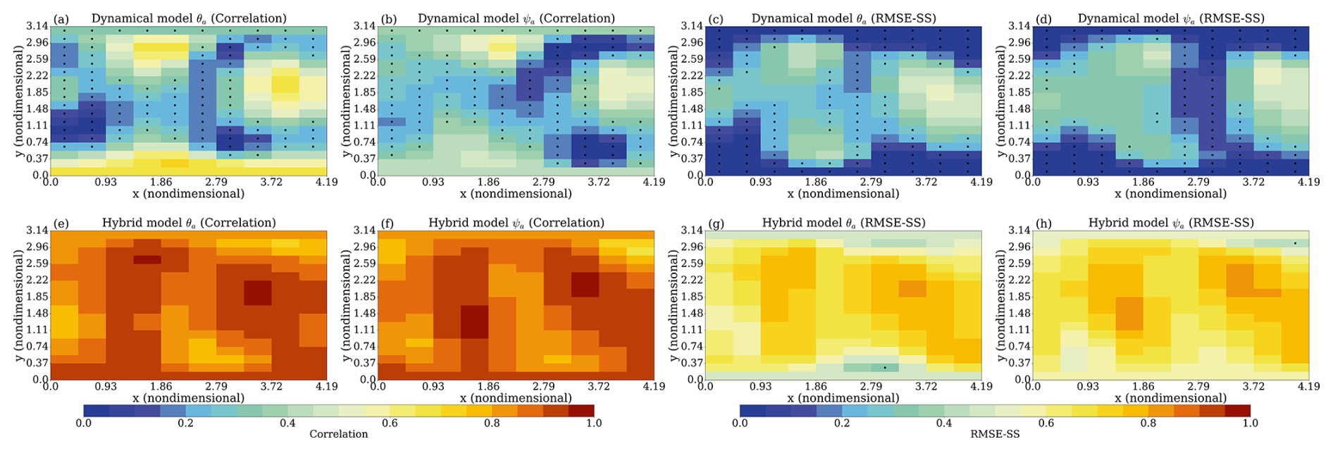
Figure 5 Spatial distributions of correlation and RMSE-SS at prediction lead day 10 for atmospheric variables. Panels (a)–(d) show results from the dynamical climate model: (a) correlation between predicted and observed atmospheric temperature; (b) correlation for atmospheric streamfunction; (c) RMSE-SS for atmospheric temperature; and (d) RMSE-SS for atmospheric streamfunction. Panels (e)–(h) show corresponding results from the hybrid model. The black dot indicates the correlation and RMSE-SS does not exceed the 95 % significance test.

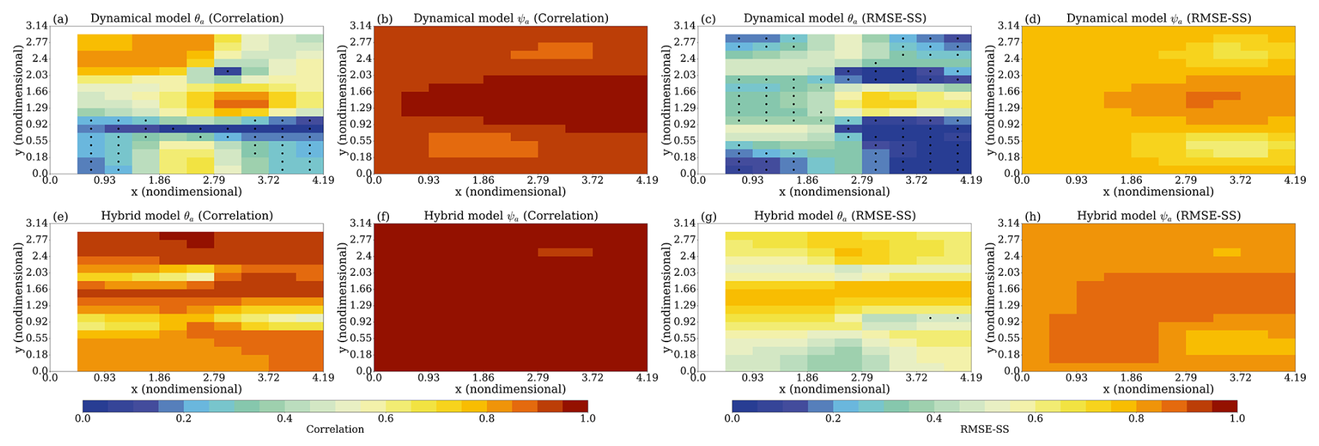
Figure 6 Spatial distributions of correlation and RMSE-SS at prediction lead year 40 for oceanic variables. Panels (a)–(d) show results from the dynamical climate model: (a) correlation between predicted and observed oceanic temperature; (b) correlation for oceanic streamfunction; (c) RMSE-SS for oceanic temperature; and (d) RMSE-SS for oceanic streamfunction. Panels (e)–(h) show corresponding results from the hybrid model. The black dot indicates the correlation and RMSE-SS does not exceed the 95 % significance test.

For atmospheric variables, both atmospheric streamfunction and temperature exhibit similar spatial characteristics (Fig. 5). We find that the hybrid model has similar spatial patterns but outperforms the dynamical climate model in most grid points.

For oceanic temperature, the dynamical climate model loses prediction skill over the majority of grid points (Fig. 6a and c). In contrast, the hybrid model demonstrates significantly higher prediction skill across most grid points (Fig. 6e and g). For oceanic streamfunction, owing to the slow nature of variability in MAOOAM, the dynamical climate model retains high prediction skill at all grid points even at a 40-year lead time (Fig. 6b and d). The hybrid model further improves upon this, showing higher correlations and RMSE-SS at all grid points, thereby outperforming the dynamical climate model (Fig. 6f and h).

For long-term climate prediction, there are additional requirements that the hybrid model must meet. Specifically, the model should be capable of running for extended periods without diverging or exhibiting significant physical instability. In our study, we find that the hybrid model maintains stability and does not experience significant physical instability during the 60-year prediction period.

In summary, the overall performance of the hybrid model surpasses that of the dynamical climate model in both spectral and physical space, demonstrating the advantages of incorporating a data-driven error correction model constructed by ML. This result highlights the potential benefits of leveraging data-driven approaches to improve climate prediction skills.

3.2 Importance of atmospheric or oceanic error correction

In this section, we extend our analysis by constructing two additional hybrid models to explore the influence of correcting atmospheric and oceanic errors separately. These models are trained using the same inputs as in the previous section, but are designed to correct either atmospheric errors or oceanic errors. By comparing the prediction skills of the regional averaged variables in physical space among these hybrid models, we gain some insight into the relative importance of atmospheric and oceanic error correction for the overall performance of the climate prediction on different time scales.

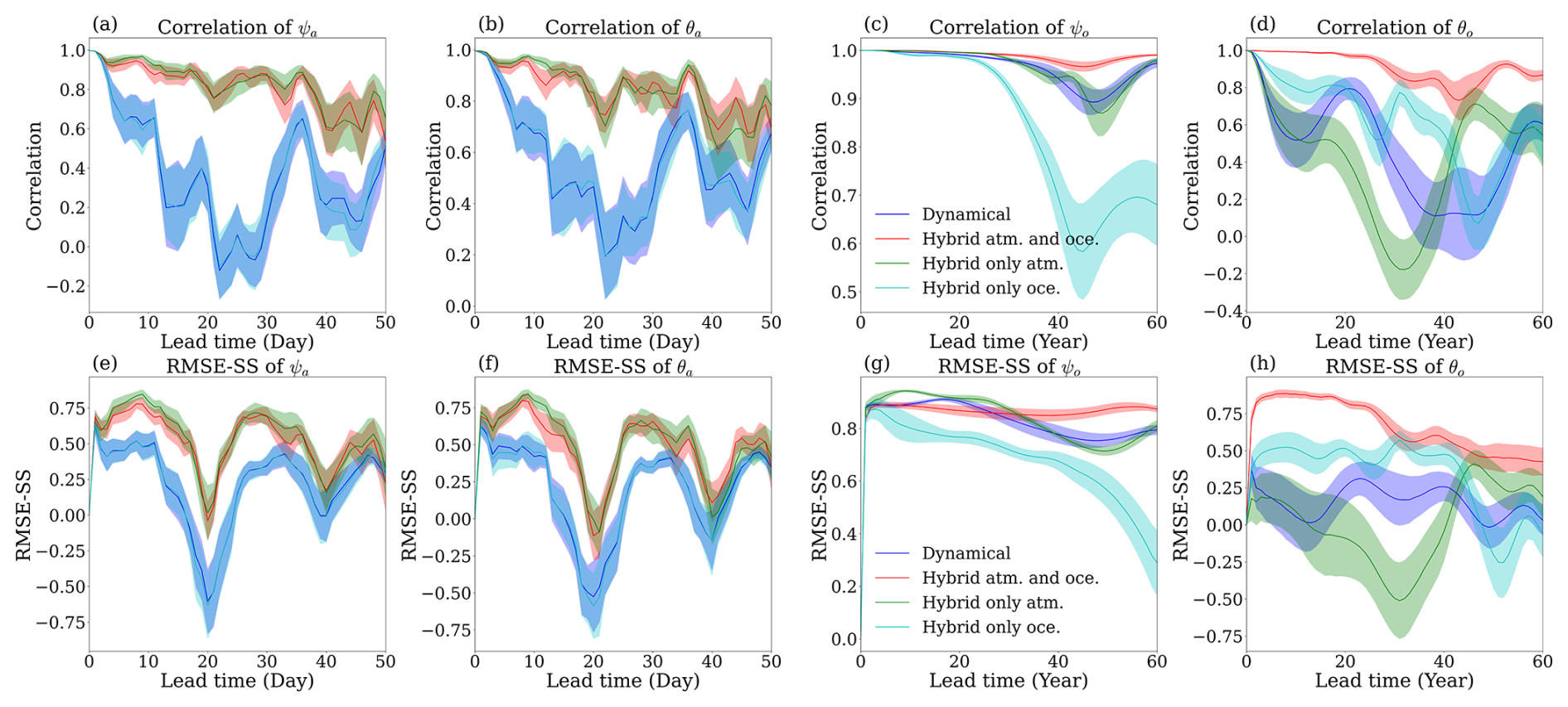
Figure 7 Correlation (a–d) and RMSE-SS (e–h) as a function of lead time (50 d for the atmospheric variable and 60 years for the oceanic variables). Shading shows one standard deviation calculated by the bootstrap method described in Sect. 2.5. The red line is the correlation/RMSE-SS of the hybrid model built by correcting both atmospheric and oceanic model errors, the green line is the correlation/RMSE-SS of the hybrid model built by only correcting atmospheric model errors, the cyan line is the correlation/RMSE-SS of the hybrid model built by only correcting oceanic model errors and the blue line is the correlation/RMSE-SS of the dynamical climate model.

In Fig. 7a, b, e, and f, we present the correlation and RMSE-SS of different models specifically for the atmospheric streamfunction and temperature. We observe that there is minimal difference in prediction skill between correcting only the atmospheric errors (green line) and correcting both the atmospheric and oceanic errors (red line). However, in the early prediction period (less than 20 d), correcting only atmospheric errors has slightly higher skills than correcting both atmospheric and oceanic errors simultaneously. When comparing the hybrid models with the dynamical climate model (blue line), we find that correcting only the oceanic errors (cyan line) does not lead to improvements in atmospheric prediction. It is related to the fact in MAOOAM that the atmosphere mostly drives the ocean but the ocean has too weak influence on the atmosphere for short-term climate prediction (Jung and Vitart, 2006).

In Fig. 7c, d, g and h, we focus on the long-term prediction skill of various hybrid models for the oceanic streamfunction and temperature. Our results reveal that the highest prediction skill over 60 years is achieved when both atmospheric and oceanic errors are corrected (red line). The hybrid models constructed by correcting only atmospheric or oceanic model errors exhibit different performances. For the oceanic streamfunction (Fig. 7c, g), correcting only oceanic errors (cyan line) does not improve prediction skill. As lead time increases, both the correlation and RMSE-SS metrics indicate a degradation in performance, with skill levels even lower than the dynamical climate model (blue line). In contrast, correcting only atmospheric errors (green line) significantly improves prediction skill within the first 20 years. However, beyond 20–30 years, the skill gradually declines and becomes comparable to that of the dynamical climate model. Notably, the hybrid correction that simultaneously addresses both atmospheric and oceanic model errors (red line) consistently outperforms the dynamical climate model after 30 years, in both correlation and RMSE-SS metrics.

Regarding oceanic temperature (Fig. 7d and h), correcting only atmospheric errors does not improve the prediction of oceanic temperatures, while only correcting oceanic errors can enhance the prediction skill of oceanic temperatures. Additionally, simultaneously correcting both atmospheric and oceanic errors (red line) can achieve the highest prediction skills at all lead times.

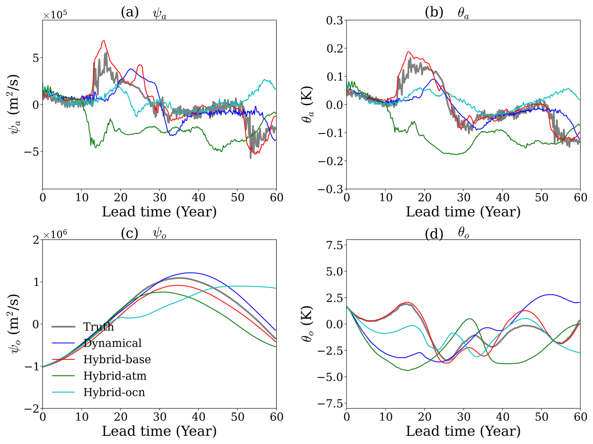
Figure 8 A case study based on the ensemble mean and monthly mean average illustrating the simulation results of four variables averaged over the whole domain in the physical space. (a) Atmospheric streamfunction, (b) atmospheric temperature, (c) oceanic streamfunction, (d) oceanic temperature.

To better illustrate the advantages of the hybrid model, we use one prediction experiment as an example to demonstrate the benefits of correcting model errors for long-term simulations (Fig. 8). For atmospheric variables (Fig. 8a and b), correcting only one component does not effectively simulate the slow frequency atmospheric processes (i.e., low-frequency signals around lead time 20 years), while simultaneously correcting both atmospheric and oceanic model errors (red lines) can better capture this variation. For the oceanic streamfunction (Fig. 8c), solely correcting oceanic errors (cyan lines) causes a phase change compared to the truth. However, the phase of the other models still matches the truth, with some differences in magnitude and timing. For oceanic temperature (Fig. 8d), correcting only atmospheric errors leads to the largest deviation from the truth (grey lines) in the first 20 years, which is similar to the dynamical climate model. Correcting the oceanic errors is better, but still poorer than correcting both atmospheric and oceanic errors (red lines), which leads to predictions very close to the truth.

In summary, for short-term atmospheric predictions, correcting atmospheric model errors yields better results, while for long-term simulations, correcting both oceanic and atmospheric errors provides the best predictions.

4 Summary and discussions

In this study, we applied a method to online correct the error in a simplified atmosphere-ocean coupled model (MAOOAM). The errors in the MAOOAM setup stem from resolution limitations in the atmospheric component. We constructed a data-driven predictor of dynamical climate model error with ML techniques and integrated it with the dynamical climate model, creating a hybrid statistical-dynamical model. By incorporating the model error correction through the hybrid model, we significantly enhanced the prediction skills for both atmospheric and oceanic variables at different lead times in both spectral and physical space. This approach allowed us to mitigate the limitations of the dynamical climate model and achieve more accurate climate predictions.

This study also examined the respective impacts of correcting atmospheric and oceanic model errors on prediction skill. Our results indicate that short-term atmospheric predictions are primarily influenced by atmospheric model errors, while correcting oceanic errors alone has a limited effect (e.g., Balmaseda and Anderson, 2009). For long-term ocean prediction, correcting atmospheric errors is essential due to their role in surface forcing, while correcting oceanic errors plays a more critical role in predicting ocean temperature. It is worth noting that in our experiment setup, the ocean component is perfect, and its prediction errors primarily come from the errors in the atmospheric component. However, correcting the ocean model errors can influence the atmosphere through the coupling between the ocean and the atmosphere. Although the experimental setup is not ideal, our results still provide some insights into the relative importance of oceanic error correction for the prediction on different time scales.

This study serves as a proof of concept, demonstrating the potential of using ML to learn and correct errors in dynamical climate models, thereby enhancing their prediction skills. Although conducted in the simplified atmosphere-ocean coupled model MAOOAM, this study contributes to the understanding of the impact of correcting model errors on climate prediction in the atmosphere-ocean coupling process. It emphasizes the importance of errors in different components of coupled models and highlights how correcting errors in various components can improve predictions on different time scales. Future applications involve applying this method to realistic climate models, which are inherently more complex than MAOOAM, and exploring the prediction skills under such conditions.