Ensemble-based model predictive control using data assimilation techniques

Model predictive control (MPC) is an optimization-based control framework for linear and nonlinear systems. MPC estimates control inputs by iterative optimization of a cost function that minimizes deviations from a desired state while accounting for control costs over a finite prediction horizon. This process typically involves direct computations in state space through full model evaluations, making it computationally expensive for high-dimensional nonlinear systems. This study introduces ensemble-based model predictive control (EnMPC), a novel framework for nonlinear control that combines MPC and ensemble data assimilation. EnMPC directly solves the MPC cost function using ensemble smoother methods, including the four-dimensional ensemble variational assimilation method, ensemble Kalman smoother, and particle smoother. By assimilating objective outputs that incorporate information about reference trajectories and constraints, EnMPC mitigates nonlinearity and uncertainty, outperforming conventional MPC in terms of computational efficiency through ensemble approximations. In addition, EnMPC is able to determine optimal weights for control inputs by using the analysis error covariance derived from ensemble data assimilation. We present two different approaches for defining control objectives. The penalty term approach applies penalties when model predictions violate pre-defined constraints by assimilating constraint information. In contrast, the trajectory-tracking approach assimilates outputs derived from a reference trajectory to lead the system in the direction of the desired state.

1 Introduction

The intensification of extreme weather events induced by global warming is causing significant damage to human life and property worldwide. As the IPCC sixth assessment report points out, rising temperatures increase the threat by increasing the frequency of heatwaves and heavy rains and floods and the intensity of hurricanes and typhoons (IPCC, 2021). The demand for new technological advances is growing as it becomes more difficult to manage the increasing number of extreme weather events with only infrastructure improvements. Since the middle of the 20th century, researchers have considered interventions such as cloud seeding, where they use silver iodide to induce rainfall. However, while scientific studies have provided evidence to support the effectiveness of the approach to some extent (Langmuir, 1948; Ryan and King, 1997; Silverman, 2001), its efficiency and optimization remain areas of active research.

Model predictive control (MPC) is a powerful control technique that uses dynamic models to predict future behavior and optimize control actions over a finite time horizon (Morari and Lee, 1999; Rockett and Hathway, 2017; Babu et al., 2019; Schwenzer et al., 2021). As computational power has advanced, the range of its applications has expanded, and new challenges, such as weather control, have become increasingly realistic. However, meteorological systems are highly complex, consisting of numerous interconnected elements such as the atmosphere, oceans, land, and biosphere (Lea et al., 2015; Sluka et al., 2016; Kurosawa et al., 2023). As its behavior exhibits significant nonlinearities, small variations can have unpredictable effects on the entire system (Slingo and Palmer, 2011), and the system responds slowly to interventions (Leith, 1974), making accurate predictions and control difficult. Moreover, weather models often require significant computational resources due to their high dimensionality and the need for fine temporal and spatial resolutions. Given these characteristics of weather systems, proper handling of uncertainty and the heavy computational cost of calculating optimal control inputs are key challenges for achieving effective weather control.

To properly handle uncertainty, data assimilation integrates observations and numerical models to more accurately estimate the state of the system, and this is widely used in weather forecasting (Houtekamer and Mitchell, 1998; Kalnay, 2003; Leutbecher and Palmer, 2008; Evensen, 2009). Miyoshi and Sun (2022) proposed a new experimental framework to systematically evaluate control approaches through ensemble prediction. In the framework, known as the control simulation experiment (CSE), they used ensemble data assimilation for state estimation. Subsequently, Kawasaki and Kotsuki (2024) integrated a conventional MPC method and achieved efficient control with minimal input within the CSE framework. However, the computational cost of calculating optimal control inputs remains high, and there is a need to develop more efficient control methods.

Sawada (2024a, b) proposed a weather control method that combines ensemble data assimilation and MPC, utilizing the ensemble Kalman filter (EnKF) and ensemble Kalman smoother (EnKS) to solve the MPC problem efficiently. Traditional MPC requires direct computations in state spaces and explicit calculations of system evolution within the prediction horizon, whereas ensemble approximations use statistical representations, enabling more efficient control of complex systems. The EnKF-based control method, which directly utilizes the existing EnKF architecture, offers flexibility for geoscience applications but still faces several challenges. First, when calculating the optimal control inputs, the system's behavior within the evaluation horizon or window of the cost function is assumed to be approximately linear. In systems with strong nonlinearity, this approximation does not hold, and errors are likely to occur when calculating the optimal control input (Zhang et al., 2009; Kurosawa and Poterjoy, 2021). Second, as used in Sawada (2024a), many control problems commonly add penalty terms to the cost function to handle constraint violations in control objectives. In the penalty-based approaches, when control objectives are complex or involve trade-offs between multiple competing goals, designing the cost function and setting penalties become challenging, potentially reducing performance and causing unintended behavior.

To address these challenges, the current study extends the methodology of using ensemble data assimilation for solving MPC problems, building upon the insights of Sawada (2024a). Specifically, we propose an ensemble model predictive control (EnMPC) framework that employs various ensemble data assimilation techniques, including the 4D ensemble variational method (4DEnVar), a particle filter (PF), and a particle smoother (PS). This approach expands the range of tools available for solving MPC problems in high-dimensional nonlinear systems. As part of this framework, the EnMPC includes the method proposed by Sawada (2024a), which uses the EnKF and EnKS to solve MPC problems. Furthermore, the EnMPC framework introduces not only the penalty-based approach but also a trajectory-tracking approach to achieve control, providing greater flexibility in addressing diverse control objectives. To demonstrate the effectiveness of the proposed EnMPC framework, we conduct a comparison with conventional MPC approaches.

Yamaguchi and Ravela (2023) proposed an ensemble MPC framework using fully nonlinear forward simulations and Gaussian processes for backward-gain computation. While their approach is innovative and effective for control in low-dimensional robotic systems, our proposed EnMPC framework differs in several key aspects. Specifically, we integrate ensemble-based data assimilation techniques into the control framework, allowing the assimilation of actual observations and the estimation of both the initial state and control variables. Moreover, our focus is on high-dimensional geophysical systems, where observation-based state estimation is indispensable.

The paper is organized in the following manner. Section 2 provides a brief overview of ensemble data assimilation and MPC. We introduce EnMPC in Sect. 3, and Sect. 4 describes the experimental setup. Section 5 presents the experimental results, and the last section concludes the paper with a summary of the key findings, potential applications, and directions for future research.

2 MPC and data assimilation

This section provides a brief overview of MPC and ensemble data assimilation, which constitute the proposed EnMPC framework. We begin by presenting the MPC algorithm for dealing with control problems. Subsequently, we outline ensemble data assimilation, focusing on 4DEnVar, EnKF, and the PF. This section explains MPC and data assimilation individually, while Sect. 3 highlights their similarities and differences and how they are combined to form EnMPC.

2.1 MPC

MPC is a control strategy that optimizes control inputs by using a dynamic model to predict the future behavior of the system. MPC solves an optimization problem at each time step to minimize a cost function over a finite predictive horizon. The specific design of the cost function depends on the application, but the general formulation can be expressed as follows:

$$\begin{array}{}\text{(1)}& \begin{array}{rl}J& \left({\mathit{u}}_{\mathrm{0}},{\mathit{u}}_{\mathrm{1}},\mathrm{\dots },{\mathit{u}}_{T_{\mathrm{c}}}\right)=\underset{J_{\mathrm{input}}}{\underbrace{\sum _{t=\mathrm{0}}^{T_{\mathrm{c}}}{\mathit{u}}_t^{\top }{\mathbf{C}}^{u^{-\mathrm{1}}}{\mathit{u}}_t}}\\ & +\underset{J_{\mathrm{state}}}{\underbrace{\sum _{t=\mathrm{0}}^{T_{\mathrm{p}}}{\left({\mathit{r}}_t-H^{\mathrm{c}}\left({\mathit{x}}_t\right)\right)}^{\top }{\mathbf{C}}^{r^{-\mathrm{1}}}\left({\mathit{r}}_t-H^{\mathrm{c}}\left({\mathit{x}}_t\right)\right)}}.\\ & \mathrm{s}.\mathrm{t}.{\mathit{x}}_{t+\mathrm{1}}=M_t\left({\mathit{x}}_t,{\mathit{u}}_t\right).\end{array}\end{array}$$

Here, x_t denotes the state variable at time t. The next state x_t+1 is obtained by integrating the nonlinear forecast model operator M_t forward from the current state x_t and the control input u_t. The control input cost J_input is typically optimized over a shorter control horizon T_c within the prediction horizon T_p. J_input penalizes the magnitude of the control input, preventing it from being excessively large. The state deviation cost J_state evaluates the difference between model-predicted states and the control objective r, and the optimization problem is performed over a finite prediction horizon T_p. H^c is an operator that maps the state variables x to the control variables. C^u and C^r are weighting matrices for the control input u and the deviations between state variables and the control objective, respectively. In this study, the control horizon T_c is shorter than the prediction horizon T_p, where control is applied only at the first time step of each cycle.

In conventional MPC, optimal control inputs are typically obtained by minimizing a cost function through gradient-based optimization. For nonlinear systems, this often involves solving the adjoint equations to efficiently compute gradients of the cost function with respect to control variables. Although this approach is accurate, it requires derivation and implementation of the adjoint model, which can be costly and challenging, especially for high-dimensional systems such as numerical weather prediction models.

Among the two components of the cost function in Eq. (1), the state deviation cost J_state typically has the highest computational cost. This is because it involves predicting and evaluating the future states of the system over the entire prediction horizon, which requires extensive computations, especially for complex or nonlinear systems. The ensemble approximation can mitigate this computational cost by using representative trajectories to approximate future states, as discussed in Sect. 3.

2.2 The four-dimensional variational method (4DVar) and 4DEnVar

The 4DVar method estimates the optimal initial state x₀ over a time window by considering the misfits between observations and forecast model states at multiple times. This process is achieved by minimizing the following cost function (Talagrand, 2014; Bannister, 2017):

$$\begin{array}{}\text{(2)}& \begin{array}{rl}J\left({\mathit{x}}_{\mathrm{0}}\right)& =\underset{J_{\mathrm{background}}}{\underbrace{{\left({\mathit{x}}_{\mathrm{0}}-{\mathit{x}}_{\mathrm{0}}^{\mathrm{b}}\right)}^{\top }{\mathbf{B}}^{-\mathrm{1}}\left({\mathit{x}}_{\mathrm{0}}-{\mathit{x}}_{\mathrm{0}}^{\mathrm{b}}\right)}}\\ & +\underset{J_{\mathrm{observation}}}{\underbrace{\sum _{t=\mathrm{0}}^{\mathit{\tau }}{\left({\mathit{y}}_t-H\left({\mathit{x}}_t\right)\right)}^{\top }{\mathbf{R}}^{-\mathrm{1}}\left({\mathit{y}}_t-H\left({\mathit{x}}_t\right)\right)}},\\ & \mathrm{s}.\mathrm{t}.{\mathit{x}}_{t+\mathrm{1}}=M_t\left({\mathit{x}}_t\right).\end{array}\end{array}$$

The first term in Eq. (2) qualifies the difference between the initial guess (background or prior) ${\mathit{x}}_{\mathrm{0}}^{\mathrm{b}}$ and the estimated state x₀, weighted by the background error covariance matrix B. The second term in Eq. (2) measures the misfit between the state variables and the observations y at times $t=\mathrm{0},\mathrm{1},\mathrm{2},\mathrm{\dots },\mathit{\tau }$. The observation operator H maps the state x to the observation space, and R represents the observation error covariance matrix. The time window τ is referred to as the data assimilation window and plays the same role as the prediction horizon T_p in MPC. Therefore, the second term J_observation in Eq. (2) serves a similar purpose to the state deviation cost J_state in the MPC cost function (Eq. 1) as both evaluate the discrepancies between the predicted states and the target values or observations over a specific time horizon.

Operational systems often implement 4DVar using an incremental approach to utilize the linearized model instead of the full nonlinear model (Courtier et al., 1994). Defining $\mathit{\delta }{\mathit{x}}_{\mathrm{0}}={\mathit{x}}_{\mathrm{0}}-{\mathit{x}}_{\mathrm{0}}^{\mathrm{b}}$, the cost function J(x₀) in Eq. (2) becomes

$$\begin{array}{}\text{(3)}& \begin{array}{rl}J\left(\mathit{\delta }{\mathit{x}}_{\mathrm{0}}\right)& =\underset{J_{\mathrm{background}}}{\underbrace{\mathit{\delta }{\mathit{x}}_{\mathrm{0}}^{\top }{\mathbf{B}}^{-\mathrm{1}}\mathit{\delta }{\mathit{x}}_{\mathrm{0}}}}\\ & +\underset{J_{\mathrm{observation}}}{\underbrace{\sum _{t=\mathrm{0}}^{\mathit{\tau }}{\left(\mathbf{H}\mathit{\delta }{\mathit{x}}_t-{\mathit{d}}_t\right)}^{\top }{\mathbf{R}}^{-\mathrm{1}}\left(\mathbf{H}\mathit{\delta }{\mathit{x}}_t-{\mathit{d}}_t\right)}},\\ & \mathrm{s}.\mathrm{t}.\mathit{\delta }{\mathit{x}}_{t+\mathrm{1}}={\mathbf{M}}_{\mathit{t}}\left(\mathit{\delta }{\mathit{x}}_t\right),\end{array}\end{array}$$

where M_t and H are the tangent linear operators of M_t and H, respectively. The innovation vector d_t is defined as ${\mathit{d}}_t={\mathit{y}}_t-H\left[M_t\right({\mathit{x}}_{\mathrm{0}}^{\mathrm{b}}\left)\right]$.

The convergence rate of the optimization problem depends on the condition number of the Hessian matrix (Zupanski, 1996). In operational data assimilation systems using atmospheric models, the dimension of the state vector is typically on the order of O(10¹⁰) or greater. This results in a background error covariance matrix B that is too large to be explicitly represented or handled directly. To address this computational challenge, operational systems commonly employ the following approach (Buehner, 2005; Wang et al., 2010; Zhu et al., 2022):

$$\begin{array}{}\text{(4)}& \left\{\begin{array}{l}\mathit{\delta }{\mathit{x}}_{\mathrm{0}}={\mathbf{U}}^x\mathit{v}\\ \mathbf{H}\mathit{\delta }{\mathit{x}}_t={\mathbf{U}}_t^y\mathbf{v}\end{array}\right..\end{array}$$

Here, U^x is a square root of the background error covariance matrix ($\mathbf{B}={\mathbf{U}}^x{\mathbf{U}}^{x^{\top }}$; Lorenc, 2003), and v is the new control variable in the reduced-dimension space. The initial perturbation δx₀ and the observation perturbation Hδx_t are projected onto a subspace covered by ensemble members using the transformation matrices U^x and ${\mathbf{U}}_t^y$, respectively. The perturbation matrices U^x and U^y are defined as follows:

$$\begin{array}{}\text{(5)}& \left\{\begin{array}{l}{\mathbf{U}}^x=\frac{\mathrm{1}}{\sqrt{N_{\mathrm{e}}-\mathrm{1}}}\left[\begin{array}{cccc}\mathit{\delta }{\mathit{x}}^{\left(\mathrm{1}\right)},& \mathit{\delta }{\mathit{x}}^{\left(\mathrm{2}\right)},& \mathrm{\cdots },& \mathit{\delta }{\mathit{x}}^{\left(N_{\mathrm{e}}\right)}\end{array}\right]\\ \\ {\mathbf{U}}^y=\frac{\mathrm{1}}{\sqrt{N_{\mathrm{e}}-\mathrm{1}}}\left[\begin{array}{cccc}\mathit{\delta }{\mathit{y}}^{\left(\mathrm{1}\right)},& \mathit{\delta }{\mathit{y}}^{\left(\mathrm{2}\right)},& \mathrm{\cdots },& \mathit{\delta }{\mathit{y}}^{\left(N_{\mathrm{e}}\right)}\end{array}\right]\end{array}\right.,\end{array}$$

where N_e is the ensemble size, and δx^(k) and δy^(k) are the kth ensemble perturbations for the model state and observation space, respectively. Perturbations in observation space are calculated using the tangent linear observation operator, where δy=Hδx. By adopting this transformation, the cost function is reformulated as follows:

$$\begin{array}{}\text{(6)}& J\left(\mathit{v}\right)=\underset{J_{\mathrm{background}}}{\underbrace{{\mathit{v}}^{\top }\mathit{v}}}+\underset{J_{\mathrm{observation}}}{\underbrace{\sum _{t=\mathrm{0}}^{\mathit{\tau }}{\left({\mathbf{U}}_t^y\mathit{v}-{\mathit{d}}_t\right)}^{\top }{\mathbf{R}}^{-\mathrm{1}}\left({\mathbf{U}}_t^y\mathit{v}-{\mathit{d}}_t\right)}}.\end{array}$$

To minimize Eq. (6), v must satisfy the condition $(\partial J/\partial \mathit{v}{)}^{\top }=\mathbf{0}$. As a result, this approach eliminates the need for an adjoint model as all calculations occur within the subspace covered by the ensemble samples. This incremental 4DEnVar approach, combined with ensemble-based transformations, thus balances computational efficiency and the practical constraints of high-dimensional data assimilation systems. For further details on these methods, we encourage readers to review the mathematical descriptions in Liu et al. (2009), Fairbairn et al. (2014), Poterjoy and Zhang (2015), and Kurosawa and Poterjoy (2021).

2.3 EnKF and EnKS

In this study, the control method based on the EnKF adopts the framework proposed in Sawada (2024a). The EnKF minimizes the following cost function to obtain the analysis state:

$$\begin{array}{}\text{(7)}& \begin{array}{rl}J\left({\mathit{x}}_{\mathrm{0}}\right)& =\underset{J_{\mathrm{background}}}{\underbrace{{\left({\mathit{x}}_{\mathrm{0}}-\stackrel{\mathrm{‾}}{{\mathit{x}}_{\mathrm{0}}^{\mathrm{b}}}\right)}^{\top }{{\mathbf{P}}^{\mathrm{b}}}^{-\mathrm{1}}\left({\mathit{x}}_{\mathrm{0}}-\stackrel{\mathrm{‾}}{{\mathit{x}}_{\mathrm{0}}^{\mathrm{b}}}\right)}}\\ & +\underset{J_{\mathrm{observation}}}{\underbrace{{\left({\mathit{y}}_{\mathrm{0}}-H\left({\mathit{x}}_{\mathrm{0}}\right)\right)}^{\top }{\mathbf{R}}^{-\mathrm{1}}\left({\mathit{y}}_{\mathrm{0}}-H\left({\mathit{x}}_{\mathrm{0}}\right)\right)}}.\end{array}\end{array}$$

Here, $\stackrel{\mathrm{‾}}{{\mathit{x}}_{\mathrm{0}}^{\mathrm{b}}}$ is the ensemble mean of the background state variables, and P^b represents the background error covariance matrix. As in 4DVar, MPC and EnKF consider similar cost components, taking into account the background information and discrepancies in their respective frameworks. From a variational perspective, ensemble methods like the EnKF can be interpreted as approximating the solution to a variational cost function such as Eq. (2), using ensemble statistics to represent background error covariances.

The EnKF efficiently reduces the computational cost by representing the error covariance matrix P^b statistically using ensemble members as follows (Evensen, 1994; Whitaker and Hamill, 2002; Houtekamer and Zhang, 2016):

$$\begin{array}{}\text{(8)}& {\displaystyle }& {\displaystyle }{\mathbf{P}}^{\mathrm{b}}={\mathbf{EE}}^T,\text{(9)}& {\displaystyle }& {\displaystyle }\mathbf{E}={\displaystyle \frac{\mathrm{1}}{\sqrt{N_{\mathrm{e}}-\mathrm{1}}}}\left[\mathit{\delta }{\mathit{x}}^{\left(\mathrm{1}\right)},\mathrm{\dots },\mathit{\delta }{\mathit{x}}^{\left(N_{\mathrm{e}}\right)}\right],\end{array}$$

where E is the matrix of ensemble members, with each column representing the perturbation from the forecast state. δx^(k) denotes the kth ensemble perturbations for the model state. Analytically solving the cost function in Eq. (7) yields the update of the ensemble mean. Unlike the variational methods discussed in Sect. 2.2, which require iterative numerical optimization to minimize their respective cost functions, EnKF does not require such iterations.

Regarding the update of ensemble members, we obtain the ensemble perturbation matrix X^a using the ensemble transform Kalman filter (ETKF; Bishop et al., 2001; Hunt et al., 2007), as follows:

$$\begin{array}{}\text{(10)}& {\displaystyle }& {\displaystyle }{\mathbf{X}}^{\mathrm{a}}={\mathbf{X}}^{\mathrm{b}}{\mathbf{W}}^{\mathrm{a}},\text{(11)}& {\displaystyle }& {\displaystyle }{\mathbf{W}}^{\mathrm{a}}={\left[\left(N_{\mathrm{e}}-\mathrm{1}\right){\stackrel{\mathrm{̃}}{\mathbf{P}}}^{\mathrm{a}}\right]}^{\mathrm{1}/\mathrm{2}},\text{(12)}& {\displaystyle }& {\displaystyle }{\stackrel{\mathrm{̃}}{\mathbf{P}}}^{\mathrm{a}}={\left[\left(N_{\mathrm{e}}-\mathrm{1}\right)\mathbf{I}+{\left({\mathbf{Y}}^{\mathrm{b}}\right)}^{\top }{\mathbf{R}}^{-\mathrm{1}}{\mathbf{Y}}^{\mathrm{b}}\right]}^{-\mathrm{1}}.\end{array}$$

Here, X^b denotes the background perturbations, and ${\stackrel{\mathrm{̃}}{\mathbf{P}}}^{\mathrm{a}}$ represents the analysis error covariance matrix in the transformed space. Y^b represents the perturbation of the background ensemble in the observation space, and the weights W^a are then derived based on the analysis covariance. Similarly to 4DEnVar, which uses ensemble approximations to project initial and observation perturbations onto a subspace covered by ensemble members, the ETKF efficiently reduces the dimensionality of the analysis problem with ensemble-based transformations.

Sequential methods, such as EnKF, update the state estimate as new observations become available, typically using a forecast–analysis cycle. In contrast, variational methods formulate the state estimation as an optimization problem over a time window, where the model trajectory is adjusted to minimize a cost function based on observations and prior estimates.

While EnKF is effective for real-time state estimation, EnKS improves estimation accuracy further by considering observations over a time window and incorporating their influence retrospectively. In this study, we employ 4D-ETKF as our implementation of EnKS; 4D-ETKF estimates the initial state by assimilating observations distributed over a finite time window, using an ensemble-based transformation that minimizes the analysis error covariance. Unlike the original EnKS that relies on sequential updates, 4D-ETKF applies a single batch update by linearly combining ensemble perturbations, ensuring consistency and computational efficiency without the need for adjoint models. For a comprehensive explanation, please refer to Miyoshi and Aranami (2006) and Hunt et al. (2007).

2.4 PF and PS

Variational methods and EnKF estimate the analysis state by assuming Gaussian error statistics for the background and observations and minimizing the cost functions defined in Eqs. (2) and (7). In contrast, the PF does not assume Gaussianity or linearity but approximates the entire probability distribution of the state as a set of particles (ensembles or samples). By assigning a likelihood to each particle, PF estimates the analysis state, making it suitable for systems with strong nonlinearity and non-Gaussianity. The particle distribution plays a similar role to the error covariance matrices (B and P) used in the variational methods and EnKF. Unlike these methods, however, the PF does not explicitly calculate the error covariance; instead, the particle distribution implicitly represents the statistical properties of the background error covariance. Although the likelihood function used in the PF resembles the observation term in the cost functions of other data assimilation methods, it plays a more central and explicit role in the PF.

For each particle x^(k), the likelihood is calculated as follows:

$$\begin{array}{}\text{(13)}& \begin{array}{rl}p\left(\mathit{y}|{\mathit{x}}^{\left(k\right)}\right)\propto & \exp \left(-{\displaystyle \frac{\mathrm{1}}{\mathrm{2}}}{\left(\mathit{y}-H\left({\mathit{x}}^{\left(k\right)}\right)\right)}^{\top }\right.\\ & \left.{\mathbf{R}}^{-\mathrm{1}}\left(\mathit{y}-H\left({\mathit{x}}^{\left(k\right)}\right)\right)\right).\end{array}\end{array}$$

This calculation resembles the state deviation term J_state in Eq. (1) for MPC, where posterior states are penalized based on their deviation from the reference. The likelihoods are normalized to produce the particle weights λ^(k):

$$\begin{array}{}\text{(14)}& {\mathit{\lambda }}^{\left(k\right)}={\displaystyle \frac{p\left(\mathit{y}|{\mathit{x}}^{\left(k\right)}\right)}{\sum _{m=\mathrm{1}}^{N_{\mathrm{e}}}p\left(\mathit{y}|{\mathit{x}}^{\left(m\right)}\right)}}.\end{array}$$

Using the weighted particles, the PF approximates the posterior distribution (filter distribution) as follows:

$$\begin{array}{}\text{(15)}& {\displaystyle }p\left(\mathit{x}\right|\mathit{y})\approx \sum _{m=\mathrm{1}}^{N_{\mathrm{e}}}{\mathit{\lambda }}^{\left(m\right)}\mathit{\delta }\left(\mathit{x}-{\mathit{x}}^{\left(m\right)}\right),\end{array}$$

where δ(x−x^(k)) represents a Dirac delta function centered at particle x^(k). This representation indicates that the posterior distribution is expressed as a discrete set of weighted particles. To better approximate the posterior distribution and mitigate degeneracy, where some particles have negligible weights, a resampling step is performed. During resampling, particles with higher weights are replicated, while those with lower weights are discarded, ensuring the ensemble remains focused on the most likely regions of the state space.

The PF is a method for sequentially estimating states, while the PS uses future observation data to provide more accurate state estimates. Applying the weights calculated during the filter update within a data assimilation window, the PS uses the future weights to find the smoother solution at any point throughout the window. This approach is justified by the Markov property, where the system's future evolution depends solely on its current state (Chopin and Papaspiliopoulos, 2020; Nyobe et al., 2023). By taking advantage of this feature, the smoother can produce more accurate estimates over the assimilation window by using future data and previously calculated weights.

We note that several studies propose strategies to address degeneracy and maintain particle diversity (e.g., Penny and Miyoshi, 2016; Potthast et al., 2019; Kotsuki et al., 2022). These differences include the resampling strategy, techniques to mitigate particle collapse, and localization to manage high-dimensional systems. The current study adopts the PF and PS algorithm based on the recently proposed PF by Poterjoy (2022) as it employs regularization and iterative updates to effectively address degeneracy and maintain particle diversity. For more detailed information on this approach, please refer to Poterjoy (2016, 2022) and Kurosawa and Poterjoy (2023).

3 Ensemble model predictive control

The structural similarity between estimation and control has been well established in control theory, where the full information control problem and the state estimation problem are known to be duals (Zhou et al., 1996).

Section 2 provides an overview of conventional MPC and ensemble data assimilation, highlighting their shared goal of determining optimal inputs based on the current state and future predictions. This section introduces a new control technique called EnMPC, which integrates these two methods. Since EnMPC uses the principles of data assimilation, it incorporates objective outputs that contain information about constraints and reference trajectories typically used in MPC. These objective outputs are assimilated in a manner similar to actual observations in data assimilation, allowing the cost function in EnMPC to adopt a structure similar to that in ensemble data assimilation.

Sawada (2024a) focuses on similarities and differences between EnKF and MPC and introduces EnKF-based EnMPC. Extending this concept, this section focuses on the mathematical formulation of EnMPC, using ideas from 4DVar to develop a 4DEnVar-based EnMPC approach. We define the formulation of EnMPC in a straightforward manner by modifying the MPC cost function in Eq. (1) to make it closer in structure to 4DEnVar in Eq. (6).

First, data assimilation focuses on state estimation by updating the initial conditions for model integration, while MPC estimates control inputs applied during the control horizon T_c. The proposed EnMPC framework treats the control inputs as acting only at the initial time, similarly to how data assimilation updates the initial states. While this assumption simplifies the framework, extending EnMPC to optimize control inputs over the entire control horizon T_c remains an important direction for future research. Second, we generate an objective output vector y^r. This allows EnMPC to handle reference information in the same way data assimilation incorporates observations. The cost function for EnMPC is therefore expressed as follows:

$$\begin{array}{}\text{(16)}& \begin{array}{rl}J\left({\mathit{x}}_{\mathrm{0}}\right)& =\underset{J_{\mathrm{input}}}{\underbrace{{\left({\mathit{x}}_{\mathrm{0}}-\stackrel{\mathrm{‾}}{{\mathit{x}}_{\mathrm{0}}^{\mathrm{a}}}\right)}^{\top }{\mathbf{P}}^{{\mathrm{a}}^{-\mathrm{1}}}\left({\mathit{x}}_{\mathrm{0}}-\stackrel{\mathrm{‾}}{{\mathit{x}}_{\mathrm{0}}^{\mathrm{a}}}\right)}}\\ & +\underset{J_{\mathrm{state}}}{\underbrace{\sum _{t=\mathrm{0}}^{T_{\mathrm{p}}}{\left({\mathit{y}}_t^{\mathrm{r}}-H^{\mathrm{r}}\left({\mathit{x}}_t\right)\right)}^{\top }{\mathbf{C}}^{r^{-\mathrm{1}}}\left({\mathbf{y}}_t^{\mathrm{r}}-H^{\mathrm{r}}\left({\mathit{x}}_t\right)\right)}}\\ & \mathrm{s}.\mathrm{t}.{\mathit{x}}_{t+\mathrm{1}}=M_t\left({\mathit{x}}_t\right).\end{array}\end{array}$$

Here, P^a is the analysis error covariance matrix as the ensemble updated by data assimilation can be used directly. H^r is the operator that maps the state vector to the objective output space.

In Eq. (16), the variable x₀ is optimized as the control input to guide the system's trajectory x_t toward a set of desirable future states ${\mathit{y}}_t^{\mathit{r}}$. Deviations of x₀ from the initial analysis $\stackrel{\mathrm{‾}}{{\mathit{x}}_{\mathrm{0}}^{\mathrm{a}}}$, obtained via ensemble data assimilation, are penalized to ensure that the control input remains realistic. Once the optimal control input ${\mathit{x}}_{\mathrm{0}}^{*}$ is found, the resulting trajectory x^c=argmin J(x₀) is regarded to be the controlled state.

As described in Sect. 2.2, applying ensemble approximations to the cost function in Eq. (16) yields

$$\begin{array}{}\text{(17)}& \begin{array}{rl}J\left(\mathit{v}\right)& =\underset{J_{\mathrm{input}}}{\underbrace{{\mathit{v}}^{\top }\mathit{v}}}\\ & +\underset{J_{\mathrm{state}}}{\underbrace{\sum _{t=\mathrm{0}}^{T_{\mathrm{p}}}{\left({\mathbf{U}}_t^y\mathit{v}-{\mathit{d}}_t^{\mathrm{r}}\right)}^{\top }{\mathbf{C}}^{r^{-\mathrm{1}}}\left({\mathbf{U}}_t^y\mathit{v}-{\mathit{d}}_t^{\mathrm{r}}\right)}},\end{array}\end{array}$$

where the innovation vector ${\mathit{d}}_t^{\mathrm{r}}$ is defined as ${\mathit{d}}_t^{\mathrm{r}}={\mathit{y}}_t^{\mathrm{r}}-H^{\mathrm{r}}\left[M_t\right(\stackrel{\mathrm{‾}}{{\mathit{x}}_{\mathrm{0}}^{\mathrm{a}}}\left)\right]$. The gradient of the cost function in Eq. (17) with respect to v is expressed as follows:

$$\begin{array}{}\text{(18)}& {\left({\displaystyle \frac{\partial J}{\partial \mathit{v}}}\right)}^{\top }=\mathrm{2}\mathit{v}+\mathrm{2}\sum _{t=\mathrm{0}}^{T_{\mathrm{p}}}{\mathbf{U}}^{y_t^{\top }}{\mathbf{C}}^{r^{-\mathrm{1}}}\left[{\mathbf{U}}_t^y\mathit{v}-{\mathit{d}}_t^{\mathrm{r}}\right].\end{array}$$

This expression shows that solving the EnMPC optimization problem does not require the full nonlinear model or its tangent linear model as the ensemble approximations are used to calculate the gradient.

One key advantage of ensemble-based methods over adjoint-based approaches is their suitability for parallel computation. Adjoint methods require sequential iterations between forward and backward (adjoint) models, which can be computationally demanding and less scalable. In contrast, ensemble methods allow for straightforward parallelization across ensemble members, making them highly attractive for real-time control and operational applications.

A key feature of EnMPC is its ability to assimilate objective outputs in a manner similar to actual observations in data assimilation. Therefore, the EnMPC approach, which directly solves the MPC cost function using ensemble estimations, is not limited to the 4DEnVar-based framework but can also be applied to EnKS- or PS-based frameworks. This study introduces two approaches for defining control objectives. The first, referred to as the “penalty term approach”, creates an objective output vector only when the model prediction exceeds a predefined threshold, as used in Sawada (2024a). The second, called the “trajectory-tracking approach”, generates objective outputs directly from the reference trajectory, enabling straightforward objective definition. We provide more details in Sect. 4.3. Lastly, EnMPC can appropriately handle sampling errors and uncertainties by incorporating techniques from ensemble data assimilation, such as localization and inflation, as detailed in Sawada (2024b).

4 Experimental settings

In this section, we describe the experimental setup used to evaluate the effectiveness of the proposed EnMPC through numerical experiments using the Lorenz63 (Lorenz, 1963) model. While Sect. 3 introduces the full information control assuming a known initial state, this section presents a more realistic setting where the initial condition is unknown and must be estimated using data assimilation. Our experiments follow the CSE procedure (Miyoshi and Sun, 2022; Sun et al., 2023; Ouyang et al., 2023; Kawasaki and Kotsuki, 2024; Sawada, 2024a).

4.1 Experimental procedure: coupling of data assimilation and control

Figure 1 illustrates the process of the CSE using the proposed EnMPC. The procedure consists of the following steps:

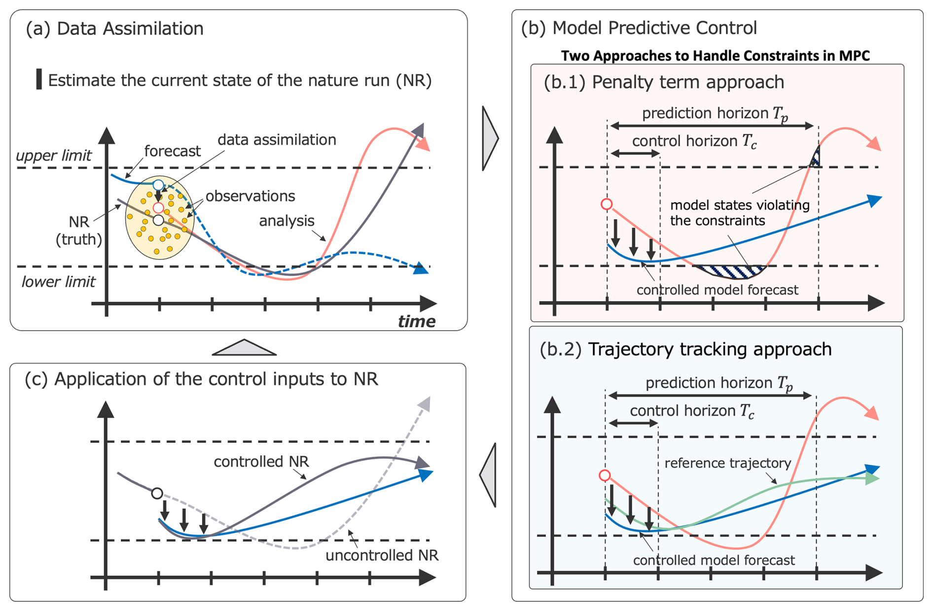
Figure 1 Algorithmic flow of the proposed EnMPC-based CSE for a system with upper and lower limits. (a) State estimation: estimates the current state of the system using data assimilation (filter update). (b) Control input optimization: determines the optimal control inputs using the proposed EnMPC framework based on ensemble forecasts; (b1) penalty term approach and (b2) trajectory-tracking approach. (c) Application of control inputs: applies the optimized control inputs to the NR, integrates the system state forward to the next time step, and returns to the filter update step (a), restarting the CSE cycle.

1. To obtain an accurate estimate of the current state of the system, we first simulate observations from the nature run (NR or the true state of the system). We then perform a conventional ensemble data assimilation using these simulated observations, which corresponds to the filter update (Fig. 1a). This step includes estimating unobserved state variables that are targets for the control. The outcome of this process provides the initial conditions necessary for the subsequent control step.

2. Based on the state estimated in the previous step, we determine the optimal control input using the proposed EnMPC. The ensemble used in the control problem is the analysis ensemble obtained through data assimilation. This ensemble reflects the flow-dependent uncertainty at the initial time and is directly employed for estimating the optimal control inputs. No additional sampling is performed specifically for the control.

   We consider two approaches for control input determination.

   • a.

     Penalty term approach. This approach uses an objective output operator, which acts as a penalty function commonly used in the conventional MPC. Objective outputs are generated when the model prediction violates the predefined constraints, effectively penalizing unsuitable behavior (Fig. 1b1).

   • b.

     Trajectory-tracking approach. In the current study, objective outputs are directly derived from the reference trajectory, making it straightforward to guide the system toward the desired state (Fig. 1b2).

3. The optimal control input determined in the second step is applied to the NR to perform the control, and the state is integrated forward to the next time step. Similarly, we apply the same control input to the ensemble members and predict their states for the next time step. With the updated system state and ensemble predictions, we restart the CSE cycle from the first step (Fig. 1c).

Here, we emphasize that, for state estimation, in the first step (Fig. 1a), we employ conventional ensemble data assimilation methods, corresponding to the filter update. In contrast, the second step (Fig. 1b) utilizes the proposed EnMPC, which is based on an ensemble smoother update, to determine the optimal control inputs. For data assimilation in the first step, we consistently use the ETKF, regardless of which ensemble smoother update method (4DEnVar, EnKS, or PS) is employed in EnMPC in the second step. This uniformity ensures that any differences in performance are solely due to the choice of method in EnMPC in the second step and not influenced by variations in the state estimation in the first step. Lastly, the current study adopts a moving-horizon window of one step. That is, regardless of the length of the prediction horizon used in EnMPC, data assimilation and control input estimation are performed at every time step in each cycle.

4.2 Model description

The current study uses the Lorenz63 (Lorenz, 1963) model for testing the proposed control method. Although relatively simple in structure, the model is widely employed as a test bed for understanding chaotic system behavior. This study aims to demonstrate the effectiveness of EnMPC for control and parameter estimation in such chaotic systems.

The Lorenz63 model is a simplified model of atmospheric convection and is represented by the following set of ordinary differential equations with three state variables:

$$\begin{array}{}\text{(19)}& \left\{\begin{array}{ll}\frac{\mathrm{d}x}{\mathrm{d}t}& =\mathit{\sigma }(y-x),\\ {\displaystyle \frac{\mathrm{d}y}{\mathrm{d}t}}& =x(\mathit{\rho }-z)-y,\\ {\displaystyle \frac{\mathrm{d}z}{\mathrm{d}t}}& =xy-\mathit{\beta }z.\end{array}\right.\end{array}$$

Following Lorenz (1963), we set the system parameters σ=10, ρ=28, and $\mathit{\beta }=\mathrm{8}/\mathrm{3}$. The time step is set to Δt=0.01 (units defined arbitrarily as 1 h; see Lorenz, 1963). The Lorenz63 model is characterized by its chaotic trajectory, which oscillates around two unstable fixed points, $(\pm \sqrt{\mathrm{72}},\pm \sqrt{\mathrm{72}},\mathrm{27}{)}^{\top }$ (Kaiser et al., 2018).

Using the Lorenz63 model, the current study investigates two scenarios for control input estimation: estimating only u_x, as shown in Eq. (20), and estimating all three control variables u_x, u_y, and u_z, as shown in Eq. (21):

$$\begin{array}{}\text{(20)}& \left\{\begin{array}{ll}\frac{\mathrm{d}x}{\mathrm{d}t}& =\mathit{\sigma }(y-x)+u_x,\\ {\displaystyle \frac{\mathrm{d}y}{\mathrm{d}t}}& =x(\mathit{\rho }-z)-y,\\ {\displaystyle \frac{\mathrm{d}z}{\mathrm{d}t}}& =xy-\mathit{\beta }z,\end{array}\right.\end{array}$$

and

$$\begin{array}{}\text{(21)}& \left\{\begin{array}{ll}\frac{\mathrm{d}x}{\mathrm{d}t}& =\mathit{\sigma }(y-x)+u_x,\\ {\displaystyle \frac{\mathrm{d}y}{\mathrm{d}t}}& =x(\mathit{\rho }-z)-y+u_y,\\ {\displaystyle \frac{\mathrm{d}z}{\mathrm{d}t}}& =xy-\mathit{\beta }z+u_z.\end{array}\right.\end{array}$$

The control objective in the current study is to keep the value of x in the model positive, ensuring that the system avoids undesired negative states. Note that the control inputs are applied to the time derivatives of the state variables rather than the states themselves.

4.3 Objective outputs and operators

In the proposed EnMPC framework, we address control problems using two approaches: the penalty term approach and the trajectory-tracking approach. Each approach employs different methods for generating objective outputs y^r and operators H^r. Throughout our experiments, we set the objective output error covariance matrix C^r, which acts as the weighting matrix for the deviations between state variables and control objectives, to C^r=0.01I, where I is the identity matrix. This configuration is based on insights from preliminary experiments and the detailed investigation in Sawada (2024a, b).

4.3.1 Penalty term approach

In the penalty term approach, we generate objective outputs to ensure that variables remain within specified thresholds. We set the objective output value to the threshold and assimilate it into the state space via an objective output operator. Sawada (2024a) employs a similar strategy, designing the control operator to impose penalties when constraints are violated. This approach effectively makes the objective output operator serve the same role as the penalty function commonly used in conventional MPC.

The control objective of the current study is to keep the x value positive in the Lorenz63 model. When we apply the penalty term approach for the objective (as detailed in Sect. 5.1), we use the following objective output operator H^obj:

$$\begin{array}{}\text{(22)}& {\displaystyle }{H}^{\mathrm{r}}\left(x\right)={\displaystyle \frac{\log (\mathrm{1}+\exp (-ax\left)\right)}{a}},\end{array}$$

where a is a positive constant that determines the sharpness of the penalty function. As shown in Fig. 2, when a=100, the function approximates a hinge function that activates the penalty only when x becomes less than zero. To keep the value of x non-negative, we set the objective outputs as y^r=0. We then use an objective output operator H^r to project the model state x into the observation space H^r(x), effectively imposing a penalty when x violates the constraint. A smaller a results in a smoother transition, applying penalties even when x is above the threshold but approaching the threshold, as shown in Fig. 2.

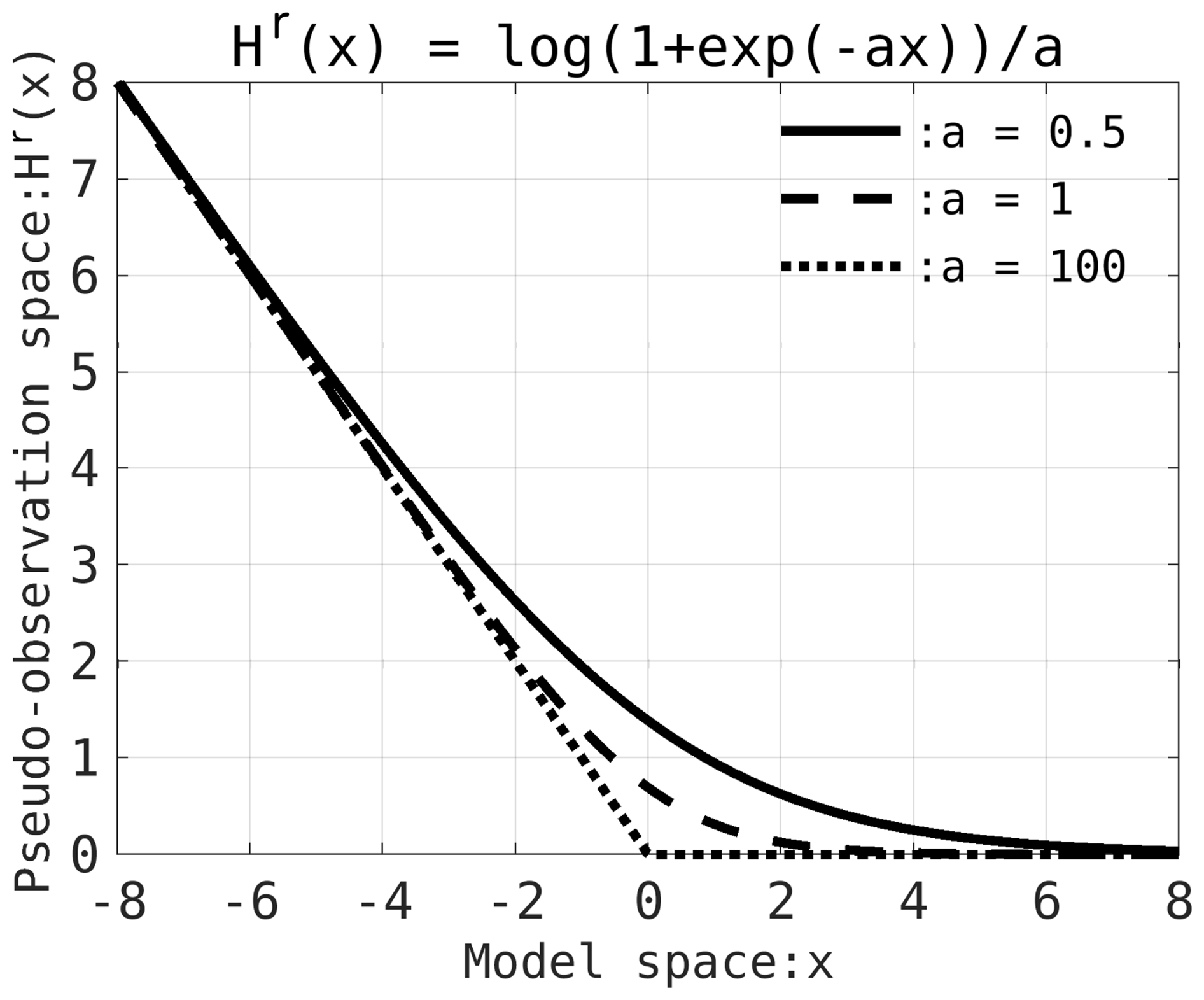
Figure 2 Comparison of the objective output operator $H^{\mathit{r}}\left(x\right)=\log (\mathrm{1}+\exp (-ax\left)\right)/a$ used in this study for different values of the positive constant parameter a. The solid line, dashed line, and dotted line represent the cases where a=0.5, a=1, and a=100, respectively. The horizontal axis represents values in the model space, while the vertical axis represents the values projected into the objective output space using the operator.

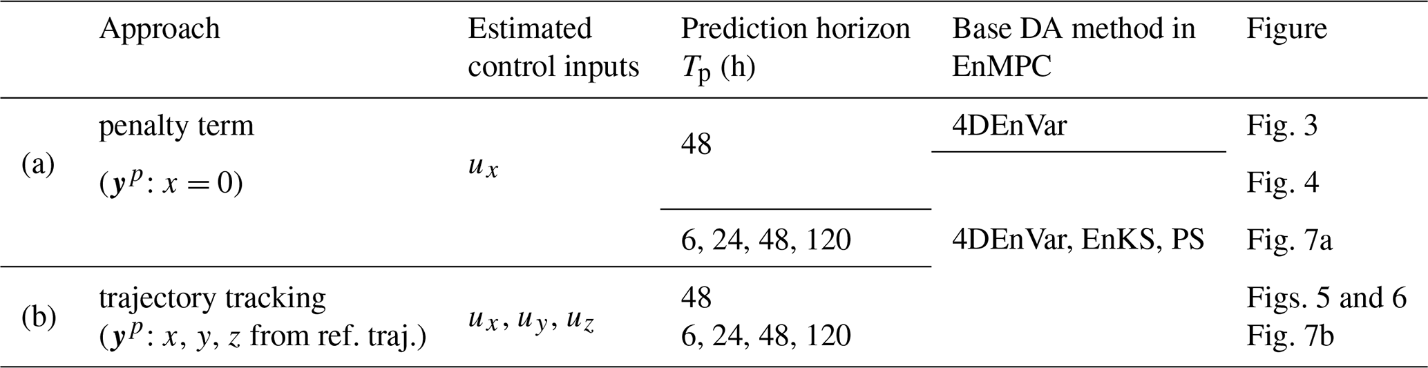
Figure 3 illustrates the impact of changing the parameter a in the objective output operator using the Lorenz63 model. Control input u_x is applied at each time step using Eq. (20), and the prediction horizon T_p is set to 48 steps (=48 h). For this demonstration, we use the 4DEnVar-based EnMPC with 10 ensemble members. The parameters for this experiment are summarized in Table 1a.

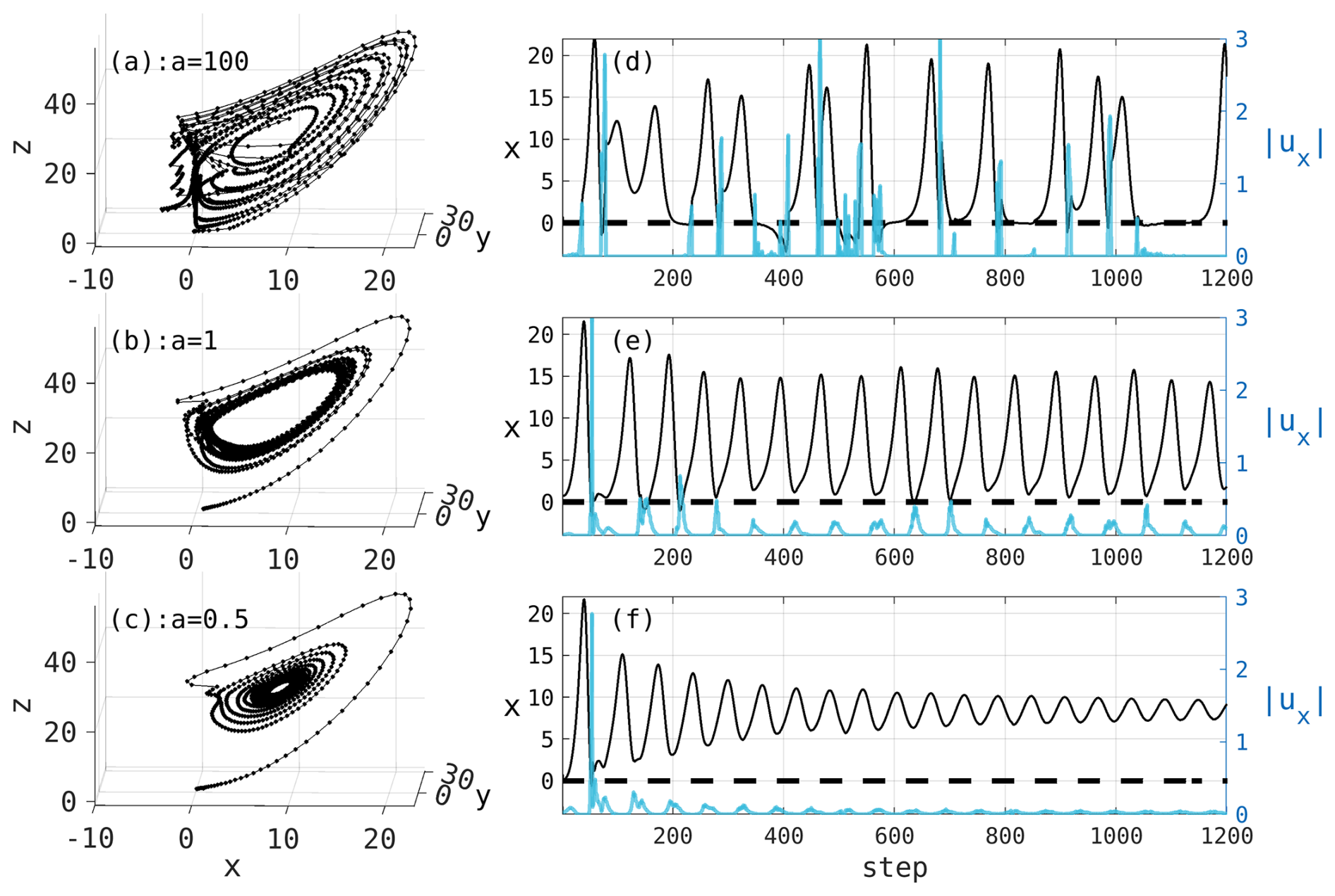
Figure 3 Comparison of results based on different values of a in the objective output operator shown in Fig. 2. The Lorenz63 model is controlled to keep the x value positive, showing the behavior over the first 1200 steps. Panels (a)–(c) show the attractors of the controlled NR for a=100, a=1, and a=0.5, respectively. Panels (d)–(f) show the evolution of x (left axis) in the controlled NR over time, with the blue lines indicating the control inputs $\left|u_x\right|$ (right axis).

Table 1 Experimental setup.

When a=100, the control inputs are relatively large due to delayed activation of the penalty term, resulting in spike-like control behavior (Fig. 3a and d). Decreasing the value of a activates the penalty more gradually, allowing the control to respond earlier, thus preventing x<0 more smoothly (Fig. 3b–c and e–f). These results show that the choice of a is critical and depends on the specific control objectives. When the control objective is to maintain the system state close to the threshold, a larger a may be necessary, leading to larger and abrupt control inputs. On the other hand, when staying further from the threshold is acceptable, a smaller a can reduce the overall control inputs, although the model states may not closely approach the threshold. This highlights the importance of selecting an appropriate objective output operator to balance the desired control objectives with the acceptable magnitude of control inputs.

4.3.2 Trajectory-tracking approach

In the trajectory-tracking approach, the current study first defines a reference trajectory that satisfies the desired constraints. We then control or guide the system to follow this trajectory by assimilating objective outputs. The objective outputs are generated by taking the states of the reference trajectory at each observation time.

For the experiment using the Lorenz63 model (as detailed in Sect. 5.2), we use the trajectory generated by Kawasaki and Kotsuki (2024) as the reference. This trajectory satisfies the constraint x>0 and is obtained using conventional MPC by applying the control inputs u_x, u_y, and u_z to the Lorenz63 model. We generate the objective outputs from the reference every time step for variables x, y, and z. The objective output operator H^r is set to the identity operator in this approach, meaning that the objective outputs directly correspond to the states of the reference trajectory without additional transformations.

5 Experimental results

In this section, we present the experimental results evaluating the performance of the proposed EnMPC using the Lorenz63 model. We compare two approaches, the penalty term approach and the trajectory-tracking approach, for the control problem of restricting the state variable x to positive values. Furthermore, we examine how the choice of methods forming the basis of EnMPC (4DEnVar, EnKS, and PS) impacts its performance. In addition, we compare EnMPC with conventional MPC to assess its computational efficiency and control performance. Note that, for the conventional MPC, we set the weighting matrix for the control input C^u to 0.01 I, which matches the objective output error covariance matrix C^r. We use an ensemble size of 10 for all experiments. All experiments are conducted using MATLAB on a typical laptop.

5.1 Control using the penalty term approach

In the penalty term approach, we restrict x to positive values by imposing penalties on regions where x≤0. Specifically, we utilize an objective output y^r=0 and a control operator $H^{\mathrm{r}}\left(x\right)=\log (\mathrm{1}+\exp (-ax\left)\right)/a$ with a=0.5. In this case, we apply the control only through u_x using Eq. (20).

As shown in Fig. 4a, while x fluctuates between positive and negative values in the NR, all four MPC methods generally restrict x to the x>0 region. This demonstrates that the proposed method successfully solves the MPC problem using ensemble approximations. In addition, the penalty term approach achieves control that takes into account constraint conditions by using the objective output operator.

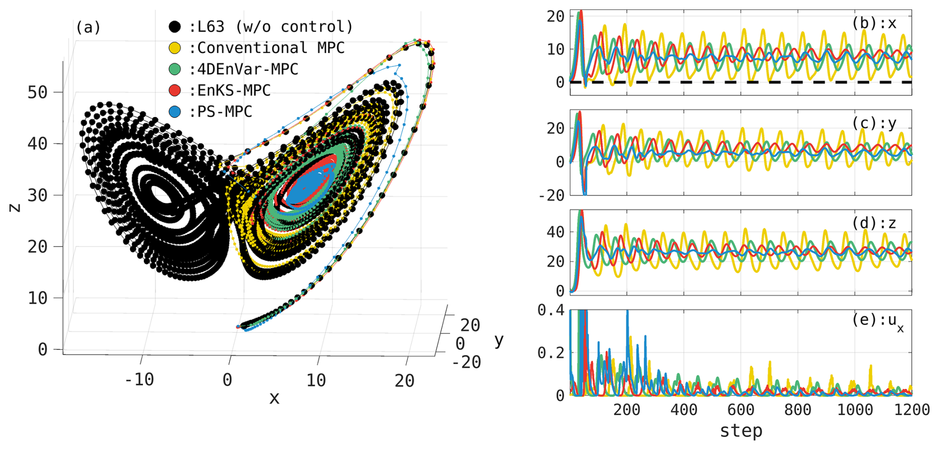
Figure 4 Comparison of results using the conventional MPC and EnMPC with the penalty term approach. (a) The trajectory of the uncontrolled and controlled NR; (b) time series of the values of x, (c) y, and (d) z in the controlled NR; and (e) the estimated control input u_x. The black dots represent the trajectory of the uncontrolled NR, and the yellow dots show controlled NR by the conventional MPC. Green, red, and blue represent the trajectories of the NR controlled by EnMPC based on 4DEnVar, EnKS, and PS, respectively. The dashed line in (b) indicates the control objective, where x>0.

The comparison of control inputs u_x shown in Fig. 4e shows that, during the initial 400 steps, the control input for EnMPC based on PS is larger than those for the other methods (4DEnVar and EnKS). As described in Sect. 2, this is because EnKS-based and 4DEnVar-based EnMPC use ensemble-based linear transformations, which help retain the statistical structure of the original ensemble (Lorenc, 2003; Poterjoy and Zhang, 2015; Houtekamer and Zhang, 2016; Kurosawa and Poterjoy, 2023). Specifically, when the cost function includes a penalty term weighted by the inverse of the ensemble covariance, the solution is guided toward regions of high ensemble density. This acts as a form of regularization, effectively constraining the solution to subspaces covered by the dominant ensemble modes and scaling it according to ensemble uncertainty (Lorenc, 2003; Houtekamer and Zhang, 2016). Compared to approaches that do not explicitly incorporate such statistical information, this often results in smaller and more dynamically consistent control inputs.

In contrast, PS-based EnMPC determines the analysis state through resampling, where particles with higher weights are replicated, while those with lower weights are removed. This can lead to the analysis state being dominated by a few specific particles, potentially causing more abrupt changes in the control input. However, this experiment uses a nonlinear observation operator $H^{\mathrm{r}}\left(x\right)=\log (\mathrm{1}+\exp (-ax\left)\right)/a$ as the penalty function, which posed challenges for EnKS-based and EnVar-based EnMPC as they inherently assume Gaussianity. On the other hand, PS-based EnMPC is more appropriate for handling non-Gaussian structures and is less affected by such assumptions (Poterjoy, 2016; Poterjoy et al., 2019; Kurosawa and Poterjoy, 2021).

Beyond step 400, the success rate of the control approaches nearly 100 % for all MPC methods, and, during this period, the magnitudes of control inputs for the three EnMPC methods show no significant differences. This suggests that the choice of data assimilation method influences the performance, especially during the initial stages.

When comparing conventional MPC and EnMPC, it becomes clear that EnMPC achieves significantly reduced control input magnitudes, which leads to smaller oscillations compared to conventional MPC. This is likely because conventional MPC uses a fixed control weight matrix C^u in Eq. (1), whereas EnMPC estimates it from the analysis ensemble as P^a in Eq. (16).

5.2 Control using the trajectory-tracking approach

The trajectory-tracking approach controls the system state toward a predefined reference trajectory that satisfies x>0. We employ the trajectory data from Kawasaki and Kotsuki (2024) as the reference and consider all three control variables u_x, u_y, and u_z using Eq. (21).

The results demonstrate that the proposed EnMPC can accurately follow the reference trajectory (Fig. 5a). In particular, 4DEnVar-based and EnKS-based EnMPC provide smooth and stable control inputs, while PS-based EnMPC requires larger control inputs (Fig. 5e–g). As mentioned in Sect. 5.1, this is because PS-based EnMPC uses particles to represent the distribution, whereas the other two methods use ensemble-based transformations. In terms of tracking performance, PS-based EnMPC achieves a significantly lower root mean squared error (RMSE) of 0.22 compared to 3.04 and 3.03 for 4DEnVar-based and EnKS-based EnMPC, respectively (Fig. 6). This suggests that the PS-based EnMPC, known for its flexibility in handling nonlinear regimes, can more accurately represent complex behaviors like the reference trajectory. In contrast, EnKS-based and EnVar-based EnMPC struggle to properly incorporate the nonlinearities of the reference trajectory, resulting in larger RMSE values.

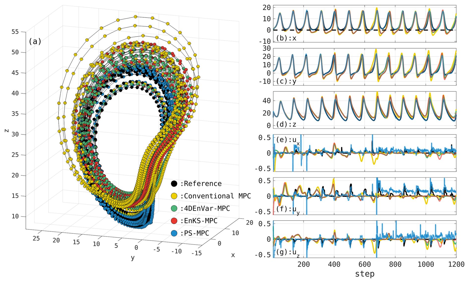
Figure 5 As in Fig. 4, but the optimal control input values are determined to follow a reference trajectory that satisfies the constraints. The black dots represent the reference trajectory.

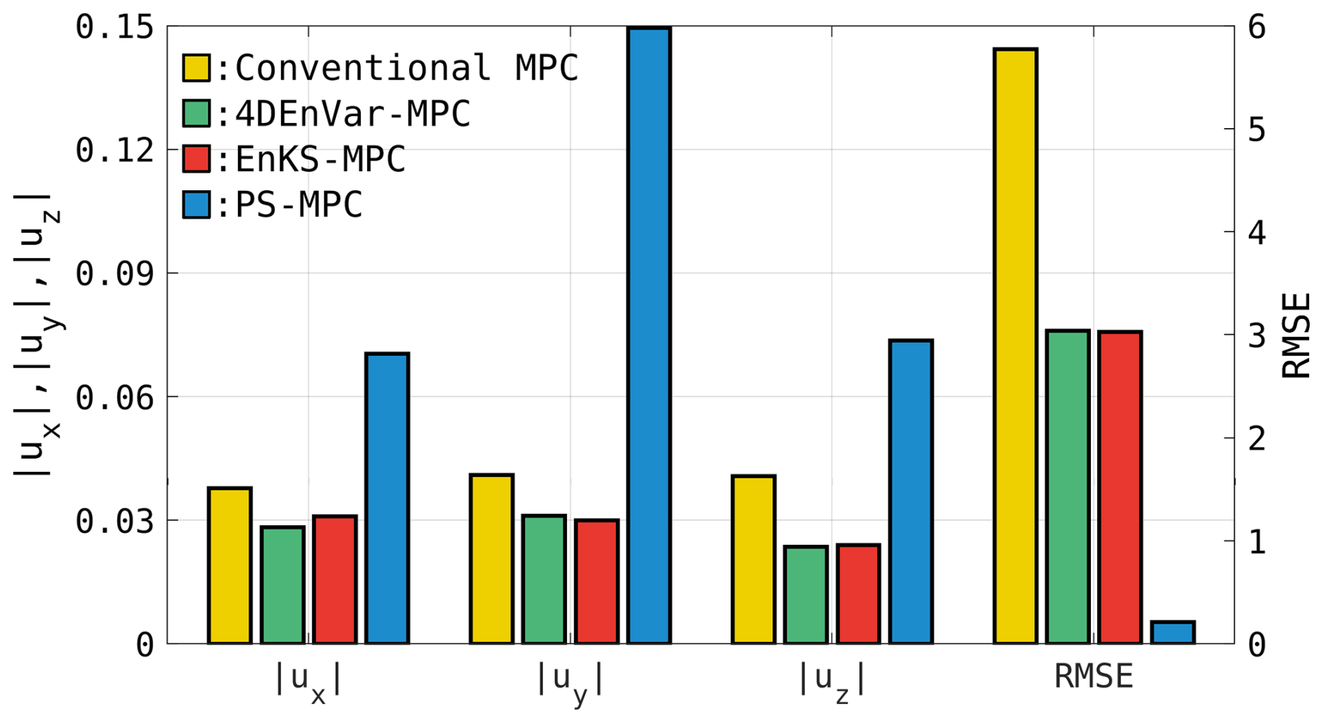
Figure 6 Comparison of the average control input magnitudes ($\left|u_x\right|$, $\left|u_y\right|$, and $\left|u_z\right|$; left axis) and RMSE (right axis) with respect to the reference trajectory, calculated as averages from step 400 to step 2000. Yellow, green, red, and blue bars represent conventional MPC, 4DEnVar-based EnMPC, EnKS-based EnMPC, and PS-based EnMPC, respectively. These values correspond to the results in Fig. 5.

When compared to conventional MPC, all EnMPC methods exhibit significant advantages in both tracking performance and control efficiency. Conventional MPC shows an RMSE of 5.91 (Fig. 6), which is considerably higher than that of any of the EnMPC methods, demonstrating its difficulty in accurately following the reference trajectory. As discussed in Sect. 5.1, this is likely to be due to the fixed control weight matrix C^u in conventional MPC, which limits its flexibility in adapting to the reference trajectory in the prediction horizon.

To enhance the accuracy of the control in both conventional MPC and EnMPC or to reduce the abrupt control inputs in PS-based EnMPC, improving the prediction horizon or increasing ensemble sizes would be effective. These improvements remain an important subject for future research.

5.3 Impact of prediction horizon on computational time and control performance

This section provides a comparison of the computational time required by conventional MPC and various EnMPC methods across different prediction horizons (T_p). We perform the comparison for both the penalty term approach (Fig. 7a) and the trajectory-tracking approach (Fig. 7b). The success rate in Fig. 7a is computed as the proportion of time steps – excluding the initial 200 spin-up steps – during which the value of x remains positive.

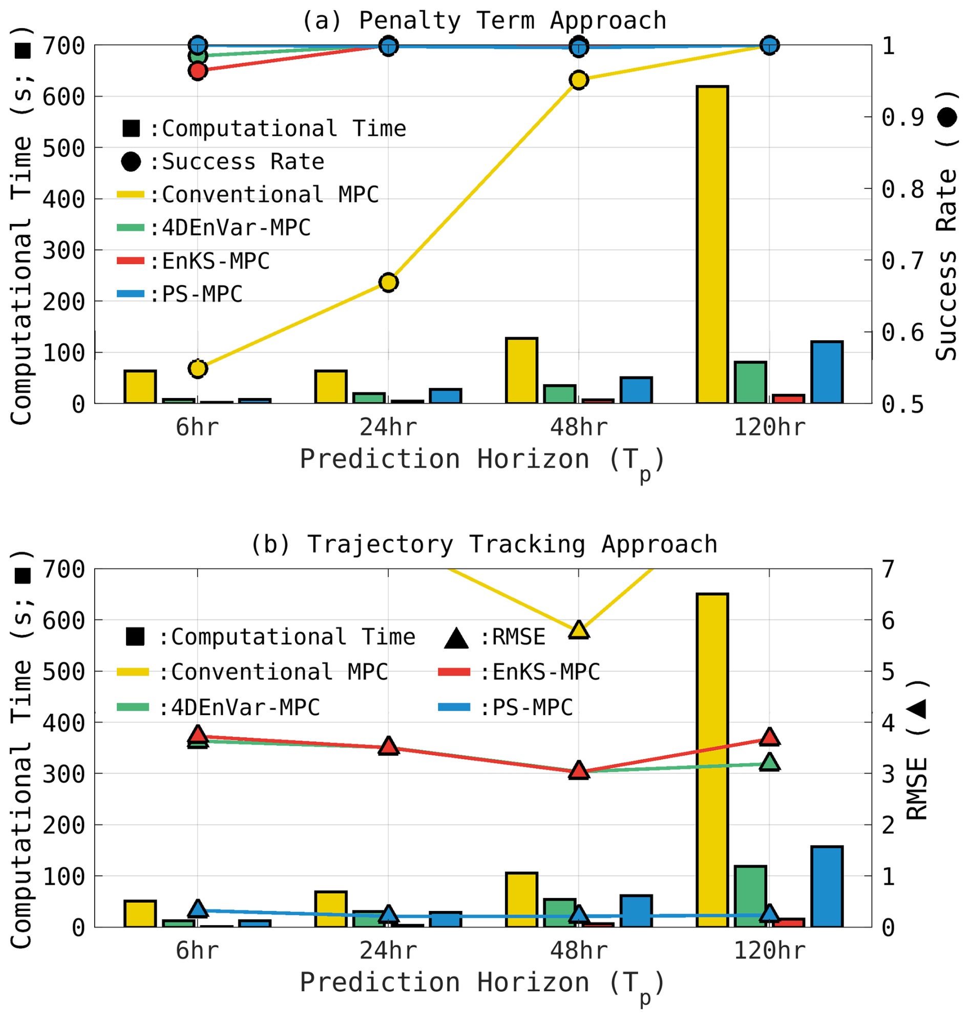
Figure 7 Comparison of computational time and performance metrics (success rate and RMSE) as a function of the prediction horizon (T_p). Panel (a) shows the penalty term approach, depicting computational time (bars, left axis) and success rate (circles, right axis), where a higher success rate indicates more effective control. Panel (b) illustrates the trajectory-tracking approach, highlighting computational time (bars, left axis) and RMSE (triangles, right axis), where a lower RMSE indicates more accurate tracking of the reference trajectory. Yellow, green, red, and blue bars represent conventional MPC, 4DEnVar-based EnMPC, EnKS-based EnMPC, and PS-based EnMPC, respectively. The values for T_p=48 h in panel (a) and (b) correspond to the results presented in Figs. 4 and 5, respectively.

In the penalty term approach (Fig. 7a), EnMPC methods consistently achieve high success rates (approximately 1.0) across all prediction horizons. In contrast, conventional MPC fails to control effectively when the prediction horizon is short (6 and 24 h). In terms of computational time, conventional MPC exhibits a sharp increase as T_p extends, reflecting its computational inefficiency due to the need for full-model evaluations to calculate optimal control inputs. For example, at T_p=120 h, the computational time for conventional MPC is 620 s. On the other hand, the EnMPC methods all show much lower computational times, with the PS-based approach yielding 121 s, the 4DEnVar-based approach yielding 81 s, and the EnKF-based approach being the most computationally efficient at 16 s. This is because the 4DEnVar and PS methods used in the current study require iterations to determine the optimal control inputs, whereas EnKS does not. Exploring alternative data assimilation methods to further reduce computational time remains an important future research topic.

For the trajectory-tracking approach (Fig. 7b), the PS-based EnMPC achieves the lowest RMSE, maintaining high control accuracy across all prediction horizons. This is because PS does not assume Gaussianity and effectively handles the nonlinear regime, making it well-suited for accurately representing complex reference trajectories. In contrast, conventional MPC exhibits significantly higher RMSE values, indicating difficulty in tracking the reference trajectory, regardless of T_p. In terms of computational time, PS-based EnMPC requires slightly higher computational costs compared to other EnMPC methods, but it remains much more efficient than conventional MPC (e.g., at T_p=120 h: conventional MPC = 651 s, 4DEnVar-based = 119 s, EnKF-based = 16 s, PS-based = 158 s). This suggests that PS-based EnMPC is a strong candidate for applications where high control accuracy is prioritized. Note that the relatively higher computational cost of PS-based EnMPC in this study is due to the iterative approach used to prevent particle degeneracy (Poterjoy et al., 2019; Poterjoy, 2022). Alternative PF or PS formulations may reduce computational costs while maintaining performance (Penny and Miyoshi, 2016; van Leeuwen et al., 2019; Kotsuki et al., 2022).

In summary, these results demonstrate that EnMPC outperforms conventional MPC in terms of both computational efficiency and control performance. Particularly for longer prediction horizons, EnMPC effectively limits computational cost increases while maintaining high control accuracy.

6 Conclusion

The current study proposes EnMPC, a nonlinear control framework that combines MPC with ensemble data assimilation. EnMPC reduces computational cost while maintaining accurate control of nonlinear systems by using ensemble approximation. EnMPC assimilates objective outputs in a manner similar to actual observations in data assimilation to reflect constraints or reference trajectories of control problems. This unique approach provides an effective and flexible solution for addressing the challenges posed by complex and high-dimensional systems, such as those in meteorology and weather control.

We introduce two methods within the EnMPC framework: the penalty term approach and the trajectory-tracking approach. The penalty term approach imposes penalties when the system violates constraints, ensuring the system remains within acceptable behavior. In contrast, the trajectory-tracking approach guides the system to follow a pre-defined trajectory that is designed to satisfy the constraints. Both approaches demonstrate their effectiveness in controlling the chaotic dynamics of the Lorenz63 model, showing their potential to manage complex system behavior and their adaptability to diverse control objectives. The choice between these two approaches depends on the specific control problem. Selecting the appropriate method based on its characteristics and objectives is essential and remains a key area for future research.

Our experiments highlight the strengths of EnMPC compared to conventional MPC, particularly in terms of computational efficiency and flexibility. This advantage is primarily due to the fact that conventional MPC relies on the full model for optimization, whereas EnMPC uses ensemble approximations. Additionally, EnMPC determines the weights for control inputs using the analysis error covariance derived from ensemble data assimilation, while conventional MPC uses fixed control weights, limiting its adaptability to varying system dynamics.

A key aspect of our investigation involves exploring the performance of different ensemble data assimilation methods that form the foundation of the EnMPC framework, which highlights the importance of selecting the appropriate ensemble smoother method, such as 4DEnVar, EnKS, and/or the PS. For instance, while 4DEnVar-based and EnKS-based EnMPC provide smooth and efficient control, the flexibility of PS-based EnMPC in handling nonlinear and non-Gaussian dynamics leads to greater accuracy, particularly when tracking nonlinear reference trajectories.

In particular, ensemble methods including PFs can be adapted to higher-dimensional settings by introducing localization techniques, as demonstrated in prior data assimilation studies. While PFs face challenges such as degeneracy in high-dimensional spaces, recent advances in localized and hybrid PF approaches offer promising directions for overcoming these limitations.

Despite its advantages, EnMPC is sensitive to factors such as the objective outputs, prediction horizon, ensemble size, and the choice of data assimilation method. For instance, achieving optimal performance with the penalty term approach requires careful tuning of objective output operators. The sensitivities highlight the need for further investigation and optimization to enhance the effectiveness and applicability of EnMPC.

In conclusion, EnMPC represents a promising framework for controlling chaotic and nonlinear systems. While our current validation is based on the simplified model, future work will explore its applicability to more complex, high-dimensional systems. These include not only operational weather models but also other nonlinear dynamical systems such as ocean circulation models, ecosystem dynamics, and economic or neural systems. Addressing key challenges – such as improving computational efficiency, optimizing parameter selection, and mitigating sampling errors – will be essential for these extensions. EnMPC thus holds potential as a powerful tool for diverse applications in the middle to long term, including but not limited to weather control.