Ionospheric chaos in the solar quiet current due to sudden stratospheric warming events across the European and African sectors

This study examines the ionospheric chaos in the solar quiet current, S_q(H), across European and African sectors during 2009 and 2021 sudden stratospheric warming (SSW) events. The SSW was categorized into precondition, ascending, peak, descending, after-, and no-SSW phases based on the rising stratospheric temperature. 13 magnetometer stations, located within the geographical longitude of 26 to 40° across European and African sectors were considered. The magnetometer data obtained during the periods of SSW were used to derive the solar quiet current time series. This solar quiet current time series was transformed into a complex network using the horizontal visibility graph (HVG) approach, and fuzzy entropy (FuzzyEn) was applied to the resulting node-degree time series to quantify the presence of chaos or orderliness behavior in the ionosphere during SSW. The results revealed that the latitudinal distribution of entropy in the European sector depicts high entropy values, indicating the presence of ionospheric chaos. Consistent low entropy values unveiling the presence of orderliness behavior were found to be prominent in the African sector. This dominance of orderliness behavior during the phases of SSW in the African sector reveals that the SSW effect manifest orderliness behavior on the regional ionosphere of the African sector, while the pronounced features of ionospheric chaos found in the European sector reveal evidence of significant effects of SSW on the regional ionosphere in this sector. Finally, we found that after the peak phase of SSW, the ionospheric chaos is more pronounced.

1 Introduction

The chaotic behavior of the ionosphere dominates due to the complex interaction between the lower- and upper-atmospheric circulation. This complex interaction is influenced by geographical location, solar activity, and atmospheric dynamics. One of the lower-atmospheric events capable of causing global disruptions to the ionosphere is sudden stratospheric warming (SSW). SSW is one of the usual meteorological events, where the stratospheric temperature increases rapidly in the winter polar region due to the rapid growth of quasi-stationary planetary waves from the troposphere (Baldwin et al., 2021; Butler et al., 2015). The connections between the troposphere and stratosphere during SSW introduce upward wave energy propagation that can reshape the plasma density variability in the ionosphere. The dominant mechanisms facilitating the connection of these processes include planetary waves, atmospheric tides, and gravity waves (Goncharenko et al., 2021; Chau et al., 2012; Goncharenko et al., 2010, 2012; Liu et al., 2010). Also, other external sources that could facilitates SSWs are heliospheric plasma sheet (HPS) and magnetosphere interaction. This occur when HPS impinges on the magnetosphere, compressing it and accelerates protons, which in turn generate electromagnetic ion cyclotron (EMIC) waves. These waves interact with relativistic electrons, causing their rapid loss to the atmosphere, potentially affecting the climate mechanism (Tsurutani et al., 2016; Liu et al., 2022).

The SSW effect introduces spatial and temporal variability in the ionospheric plasma density (Yamazaki, 2013, 2014; Klimenko et al., 2018). As a result, the ionosphere exhibits nonlinear dynamical behavior characterized by high sensitivity to minor perturbations originating from the lower and upper atmosphere that could lead to transitions between orderliness and chaotic behavior of ionosphere, rendering its state susceptible to sudden and significant changes.

In the studies of dynamical systems, such as logistic map, chaotic behavior is strongly associated with high entropy measurements, while orderliness behavior is associated with a declining and low entropy measurements (Conejero et al., 2024). This observation forms the basis of this study to quantitatively examine the dynamical behavior of the ionosphere during SSW across European and African sectors. The regional ionosphere of European and African sectors manifests pronounced ionospheric variability in response to SSW events. For example, proximity to the geomagnetic Equator in Africa could lead to different responses compared to higher-latitude regions in Europe. This phenomenon provides a unique opportunity to investigate the complex coupling mechanisms between the stratosphere and ionosphere. Specifically, it enables the study of atmospheric wave propagation and its impact on the ionosphere, which can lead to disruptions in satellite communication and the navigation system in the region.

One of the atmospheric parameters that can reveal the extent of the SSW-induced effects on the regional ionosphere is the solar quiet current, S_q(H). During an SSW event, planetary waves and tidal interactions can generate an electromotive force that drives the ionospheric current system (Yamazaki and Richmond, 2013; Yamazaki and Maute, 2017). These ionospheric currents during geomagnetically quiet periods are referred to as solar quiet currents (S_q). They serve as a key phenomenon that manifests the degree of connection between the lower atmosphere and the ionosphere.

Several studies have already investigated the solar quiet current during an SSW (Yamazaki, 2014; Bolaji et al., 2016a; Yamazaki and Maute, 2017; Yamazaki et al., 2011). For instance, Fejer et al. (2011) found enhanced lunar semidiurnal vertical plasma drift amplitudes during early-morning solar flux warming that are associated with SSW. Maute et al. (2014) observed changes in ionospheric vertical drifts during SSW, attributing them to interactions between specific tides and planetary waves. Yamazaki et al. (2012a) studied the ionospheric current system during the 2002–2003 SSW events over east Asia, finding an additional current system superposed on the normal S_q current system. They attributed this to abnormally large lunar tidal winds, which also produced a counter electrojet (CEJ). Yamazaki et al. (2012b) examined the solar quiet current during an SSW and found significant hemispheric asymmetry: decreased intensity in the Northern Hemisphere and increased intensity in the Southern Hemisphere, accompanied by reduced longitudinal separation between the hemispheric eddies. Yamazaki (2014) studied the solar and lunar ionospheric tidal forces, which are believed to influence ionospheric electrodynamics during SSW. By analyzing the average solar and lunar ionospheric current systems during SSW and non-SSW periods, the author discovered that the intensity of lunar currents increases by roughly 75 % during SSWs, whereas the solar current intensity is only slightly diminished, by approximately 10 %. Bolaji et al. (2016b) investigated the solar quiet current response in Africa during an SSW, categorizing temperature rises into six phases. A counter electrojet formed after peak SSW, and a S_q(H) magnitude decrease between 21.13° N (Fayum, Egypt) and 39.51° S (Durban, South Africa) was observed. Siddiqui et al. (2018) examined the equatorial electrojet (EEJ) during major SSW events and found a significant increase in the amplitude of EEJ semidiurnal lunar tides during SSW. Klimenko et al. (2019) investigated the impact of the 2009 SSW on the tropical lower thermosphere–ionosphere. They found that perturbations in ionospheric conductivity significantly contribute to the electric field response to SSW. Additionally, the phase change of the semidiurnal solar tide (SW2) in neutral winds played a crucial role in shaping the zonal electric field response.

Interestingly, previous studies on solar quiet currents during SSW events did not consider the application of chaos theory. This study aims to bridge this gap by investigating the chaotic behavior of the solar quiet current system in response to SSW effects over the European and African sectors. To examine the ionosphere during 2009 and 2021 SSW events, this study utilizes a robust methodology combining two innovative techniques: the horizontal visibility graph (HVG), rooted in graph theory, to preprocess solar quiet current time series data and fuzzy entropy (FuzzyEn) analysis to reveal the underlying chaotic behavior in the ionosphere during an SSW. The reason why this study considers the combination of HVG and fuzzy entropy techniques is that fuzzy entropy is indeed robust to small-amplitude noise; some subtle features in the solar quiet current time series may still be obscured if we rely on FuzzyEn alone. The HVG transformation helps by emphasizing the “visibility” relations between data points, effectively highlighting structural patterns that may be drowned out in the raw time series. In addition, when FuzzyEn is computed on a node-degree sequence (complex network representation), it often provides clearer differentiation of regimes or subtle changes in the system that might otherwise remain hidden. Thus, combining HVG and FuzzyEn approaches can yield features more robust to measurement noise and more sensitive to underlying structural variations in the solar quiet current.

1.1 Characterization of 2009 and 2021 major SSW events

The 2009 SSW event occurred from January to March. Its rising stratospheric temperature and the corresponding stratospheric zonal mean wind was categorized into six phases during the following periods: SSW precondition phase, SSW ascending phase, SSW peak phase, SSW descending phase, after-SSW phase, and no-SSW phase (Fig. 1). The red color represents the stratospheric mean air temperature (k) at 10 hPa, while the black color is the stratospheric zonal mean wind at 10 hPa.

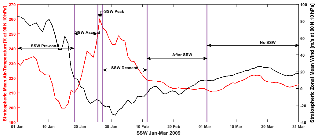
Figure 1 The stratospheric zonal mean air temperature and zonal mean wind occurring from January–March 2009, showing the SSW precondition phase, SSW ascending phase, SSW peak phase, SSW descending phase, after-SSW phase, and no-SSW phase. The stratospheric parameter during the 2009 SSW event is obtained from the National Oceanic and Atmospheric Administration (NOAA).

The SSW precondition phase represents the start of the increase in the stratospheric temperature (1–16 January) shown in Fig. 1, the SSW ascending phase signifies when the stratospheric temperature increases (17–21 January), the SSW peak phase is when the stratospheric temperature reaches its maximum (22–24 January), the SSW descending phase indicates the beginning of the stratospheric temperature decline (25 January–12 February), the after-SSW phase represents when the stratospheric temperature begins to recover to its normal state (13 February–2 March), and the no-SSW phase represents when the stratospheric temperature finally recovers to its normal state (3–31 March). The SSW event was categorized in accordance with the work of Bolaji et al. (2016b).

The stratospheric temperature and its corresponding zonal mean wind for the 2021 SSW event is shown in Fig. 2. The SSW occurred from December 2020 to February 2021 and was also categorized into six phases. The SSW precondition phase spans 1–27 December 2020, the SSW ascending phase is from 28 December 2020 to 2 January 2021, the SSW peak phase ranges from 3–5 January 2021, the SSW descending phase spans 6–14 January 2021, and the after-SSW phase is from 15 January–16 February 2021. Finally, the no-SSW phase emerges from 17–28 February 2021.

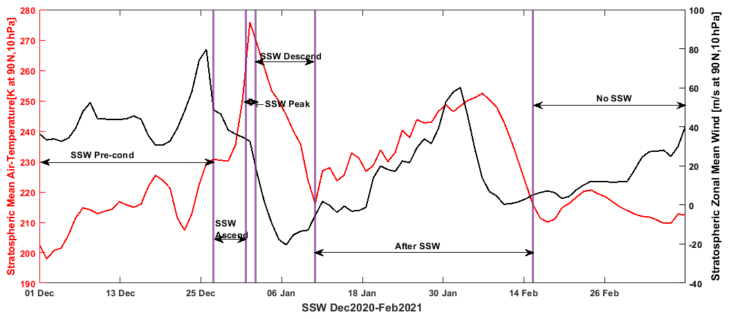
Figure 2 The stratospheric zonal mean air temperature and zonal mean wind from December 2020 until February 2021, revealing the SSW precondition phase, SSW ascending phase, SSW peak phase, SSW descending phase, after-SSW phase, and no-SSW phase. The stratospheric parameter during the 2021 SSW event is obtained from the National Oceanic and Atmospheric Administration (NOAA).

1.2 Global scale of geomagnetic activities during the 2009 and 2021 SSW events

The year 2009 was the beginning of a solar minimum of solar cycle 24, while the year 2021 was the end of solar minimum in solar cycle 24. Generally, solar minimum years are periods where the geomagnetic disturbances mostly record quiet days. This indicates that the years 2009 and 2021 of solar cycle 24 are periods where the geomagnetic disturbances were mostly minimal. The planetary index (K_p) and the solar flux activity during the months of 2009 and 2021 SSW event are shown in Figs. 3 and 4, respectively. During the 2009 SSW event (January–March), the planetary K_p index generally depicts quiet geomagnetic conditions (K_p≤3) for most days, as shown in Fig. 3. However, there were 11 exceptions (3, 19, and 26 January; 4, 14–15, 25, and 28 February; and 13 and 24 March) where K_p index values slightly exceeded 3 that were noticed within the 3 h interval range of K_p, indicating a sudden occurrence of moderate geomagnetic disturbance.

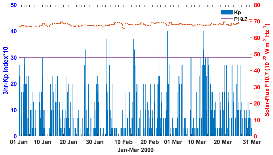
Figure 3 The planetary index K_p (blue bars) and solar flux F_10.7 (red lines) between January and March 2009. The planetary (K_p) and solar flux activity (F_10.7) during 2009 SSW periods is collected from the Space Physics Data Facility, NASA.

The planetary K_p index during the 2021 SSW event (December 2020 to February 2021), as shown in Fig. 4, generally indicated quiet geomagnetic conditions (K_p≤3) for most days, and the solar flux activity was within F_10.7∼100. However, elevated K_p index values (> 3) were observed on 16 specific days (10, 21, and 23 December; 5, 6, 11, 24, 25, and 27 January; and 2, 6, 12, 16, 20, 22, and 23 February). Because of this sudden occurrence of transient geomagnetic disturbance revealed by the K_p index in the aforementioned days during the SSW periods, in our analysis of solar quiet current derivation, we ensure that geomagnetic storm index in minutes (SYM-H) was subtracted from the H component of the magnetic field to minimize the influence of geomagnetic disturbance. However, a comparative analysis of the day-to-day geomagnetic activity in January–March 2009 and December 2020–February 2021 SSW events reveals that most days during these periods manifest K_p index values ≤ 3, indicating minimal geomagnetic activity. This observed space weather feature underscores the uniqueness of the selected SSW events for this study. An investigation into the chaotic behavior of the ionosphere during periods of low geomagnetic activity of an SSW reveals the significant impact of SSW events on ionospheric dynamics within the European and African sectors.

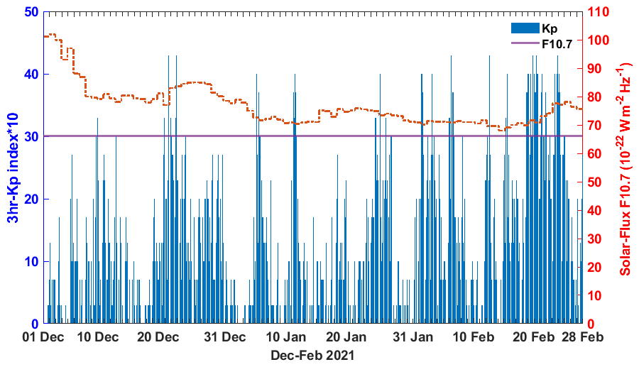
Figure 4 The planetary index K_p (blue bar) and solar flux F_10.7 (red lines) from December 2020–February 2021. The planetary (K_p) and solar flux activity (F_10.7) during 2021 SSW periods is collected from the Space Physics Data Facility, NASA.

2 Data acquisition and method of analysis

The ground-based magnetometer data acquired from the Magnetic Data Acquisition System (MAGDAS) at the International Research Centre for Space and Planetary Environment Science (i-SPES), Fukuoka, Japan (http://magdas2.serc.kyushu-u.ac.jp/, last access: 8 November 2023), is used in this study. The geographical location of the studied areas is shown in Fig. 5.

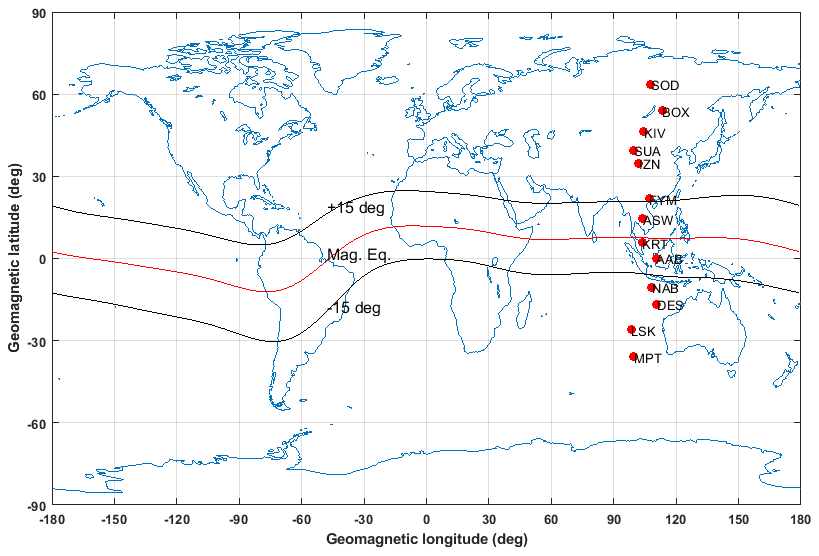
Figure 5 The geomagnetic location of the magnetometer observatories stations investigated across the European and African sectors.

The acquired magnetic data from MAGDAS covers eight magnetometer stations situated in the African sector and distributed within the geographical latitudes of both Northern and Southern Hemisphere, shown in Table 1. The geomagnetic coordinate reference year for the stations listed in Table 1 is 2009.

Table 1 Stations investigated across the European and African sectors.

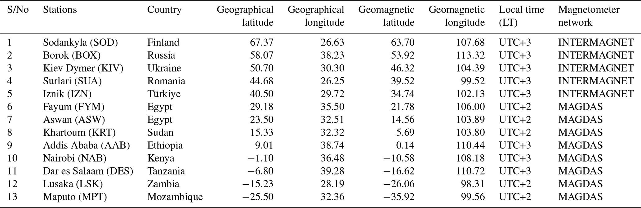
Also, magnetometer stations in Europe were acquired from the International Real-time Magnetic Observatory Network (INTERMAGNET), available online at https://www.intermagnet.org (last access: 27 December 2023). The collection consists of five magnetometer observatory stations across Europe (see Table 1). The magnetometer data were acquired during the periods of the 2009 and 2021 SSW events. Owing to the lack of magnetic data at geographical longitude between 26 and 40° in the African sector during the 2021 SSW, our study of the 2021 SSW was restricted only to the European sector.

The planetary (K_p) index during 2009 and 2021 SSW periods was downloaded from GFZ Indices of Global Geomagnetic Activity (https://www.gfz-potsdam.de/Kp-index/, last access: 12 February 2024), while the solar flux activity (F_10.7) for the 2009 and 2021 SSW periods was collected online from the archive of the Space Physics Data Facility, NASA (https://omniweb.gsfc.nasa.gov/form/dx1.html, last access: 12 February 2024).

The daily mean values of zonal mean air temperature and wind during the periods of 2009 and 2021 SSWs were acquired from the National Oceanic and Atmospheric Administration (NOAA) (https://psl.noaa.gov/data/getpage/, last access: 12 February 2024). The solar quiet current, S_q(H), was derived using the H component of the magnetic field data with a daily resolution (with the time unit in minutes). A magnetic field model (CHAOS-8.1), spanning 1999–2025, was obtained from DTU Space (https://www.space.dtu.dk/english/research/scientific_data_and_models/magnetic_field_models, last access: 17 March 2024) to determine the ionospheric field. CHAOS-8.1 is derived from magnetic field observations by low-Earth-orbiting satellites (Swarm, MSS-1, CSES, CryoSat-2, CHAMP, SAC-C, and Ørsted) and ground observatory measurements.

2.1 Derivation of solar quiet current S_q(H) time series

To derive the day-to-day S_q(H) current time series, magnetic field data from various magnetometer stations across European and African sectors were archived. We focus on acquiring magnetic field data from the magnetometer stations that are situated within the geographical longitude of 26–40°. Some of the acquired magnetic data, especially the stations in the European sector, are provided in the Cartesian (X, Y, Z) coordinate system and were converted to the geomagnetic (H, D, Z) coordinate system using the rotation matrix method (Barton and Tarlowski, 1991). We applied a magnetic field model (CHAOS-8.1) to the acquired magnetic field data to obtain the ionospheric field. The H component of the magnetic field model (CHAOS) was subtracted from the H component of the acquired magnetic data.

$$\begin{array}{}\text{(1)}& \mathrm{\Delta }H=\mathrm{\Delta }{H}_{\mathrm{magnetic}\mathrm{data}}-\mathrm{\Delta }{H}_{\mathrm{model}}\end{array}$$

To minimize the disturbance field arising from the magnetospheric currents (Bolaji et al., 2016b), the values of the geomagnetic storm index in minutes (SYM-H) were subtracted from the H component (ΔH).

$$\begin{array}{}\text{(2)}& \mathrm{\Delta }{H}_{\mathrm{local}}=\mathrm{\Delta }H-(SYM-H\times \cos \left(L\right))\end{array}$$

To estimate the solar quiet current, S_q(H), time series, the average nighttime values (in minutes) of the H component between 12:00 and 01:00 local time (LT) for a particular day, referred to as the baseline values (BLVs), were estimated using Eq. (3).

$$\begin{array}{}\text{(3)}& \mathrm{BLV}={\displaystyle \frac{\mathrm{\Delta }{H}_{\mathrm{24}}+\mathrm{\Delta }{H}_{\mathrm{01}}}{\mathrm{2}}}\end{array}$$

The notation ΔH₂₄ and ΔH₀₁ is the 60 min values of H component at 12:00 and 01:00 LT, respectively, where BLV represents the baseline value. The residual value after subtracting the baseline value from the H component gives rise to the solar quiet current time series.

$$\begin{array}{}\text{(4)}& S_{\mathrm{q}}\left(H\right)=\mathrm{\Delta }{H}_{\mathrm{local}}-\mathrm{BLV},\end{array}$$

where S_q(H) is the solar quiet current considered in minutes. The analysis of the S_q(H) was deduced for all the day-to-day activities of the 2009 SSW (January–March) and 2021 SSW (December 2020–February 2021) periods for all stations under investigation.

2.2 Detrending of solar quiet, S_q(H), current time series by the horizontal visibility graph (HVG)

The time series of the solar quiet current, S_q(H), derived during the periods of the 2009 and 2021 SSW, was subjected to the HVG method, which transforms the series into a complex network. The calculations were performed using the ts2vg Python module, specifically utilizing the HorizontalVG class, which represents one of the types of visibility graphs – namely, the horizontal visibility graph. The input to this process is a time series, which is transformed into a network where each point in the series becomes a node and edges are formed based on the visibility criteria between points (Conejero et al., 2024; Gonçalves et al., 2016; O'Pella, 2019; Luque et al., 2009; Zou et al., 2019). By applying this method, we calculate the degree (number of connections) for each point in the time series, capturing the number of other points it can see in the horizontal visibility graph. The output is a list of degrees for each point, reflecting the local connectivity structure within the time series, which helps reveal patterns, dependencies, and variability within the data. The HVG is mathematically described as follows.

Let us consider a time series of N data points be represented as

$$\begin{array}{}\text{(5)}& [x_i,i=\mathrm{1},\mathrm{2},\mathrm{\dots },N].\end{array}$$

Two nodes, i and j, in the graph are connected if it is possible to trace a horizontal line in the series linking x_i and x_j not intersecting intermediate data height, fulfilling

$$\begin{array}{}\text{(6)}& x_i,x_j>x_n\text{for all}i<n<j.\end{array}$$

2.3 Fuzzy entropy (FuzzyEn)

Fuzzy entropy (FuzzyEn) is a powerful and popular nonlinear tool used to assess the dynamical characteristics of time series data (Ishikawa and Mieno, 1979; Li et al., 2017; Azami et al., 2019; Chen et al., 2007). It provides a quantitative measure of a signal's complexity and chaos. High entropy indicates more irregular (chaotic) dynamics, whereas low entropy suggests a more regular or periodic nature. FuzzyEn was developed to overcome the shortcoming of approximate entropy (ApEn) and sample entropy (SampEn) (Azami et al., 2019; Li et al., 2017; Dass et al., 2019). FuzzyEn uses exponential functions with fuzzy boundaries. It is expressed mathematically as follows. Given a time series, we embed it using a given embedding dimension (m). Then, a new m-dimensional vector (X_m) is formed as follows:

$$\begin{array}{}\text{(7)}& {\mathit{X}}_m\left(i\right)=\left[X_i,X_{i+\mathrm{1}},\mathrm{\dots },X_N\right]-x{\mathrm{0}}_i.\end{array}$$

These vectors represent m consecutive x values, starting with the ith point and with the baseline $x{\mathrm{0}}_i=\frac{\mathrm{1}}{m}{\sum }_{j=\mathrm{0}}^{m-\mathrm{1}}{x}_{i+j}$ removed. Then, the distance between vectors X_m(i) and X_m(j), $d_{i,j,m}$, can be defined as the maximum absolute difference between their scalar components. Given n and r, the degree of similarity (D_i j, m) of the vectors X_m(i) and X_m(j) is calculated using the fuzzy function:

$$\begin{array}{}\text{(8)}& D_{i,j,m}=\mathit{\mu }\left(d_{i,j,m},r\right)=\exp \left({\displaystyle \frac{-(d_{i,j,m}{)}^n}{r}}\right),\end{array}$$

where n and r are the FuzzyEn power and threshold, respectively. The function ϕ_m is defined as

$$\begin{array}{}\text{(9)}& \begin{array}{rl}{\mathit{\varphi }}_m\left(n,r\right)& ={\displaystyle \frac{\mathrm{1}}{N-m}}{\sum }_{i=\mathrm{1}}^{N-m}\\ & \left({\displaystyle \frac{\mathrm{1}}{N-m-\mathrm{1}}}{\sum }_{\begin{array}{l}j=\mathrm{1}\\ j\ne i\end{array}}^{N-m}{D}_{i,j,m}\right).\end{array}\end{array}$$

Repeating the same procedure from Eqs. (7) and (8) for the vector X_m+1(j), i.e., for dimension m+1, the function ϕ_m+1 is obtained. Therefore, FuzzyEn can be estimated as

$$\begin{array}{}\text{(10)}& \mathrm{FuzzyEn}\left(m,n,r,N\right)=\ln {\mathit{\varphi }}_m\left(n,r\right)-\ln {\mathit{\varphi }}_{m+\mathrm{1}}(n,r).\end{array}$$

In this study, we applied the HVG and FuzzyEn to the solar quiet current, S_q(H), to investigate ionospheric chaos during SSW across the European and African sectors. The computational parameters used for FuzzyEn analysis included an embedding dimension (m=1) and a tolerance threshold defined as r₁= 0.2 × SD, where SD represents the standard deviation of the time series X. Additionally, the argument exponent (pre-division) r₂= 3 was applied along with a time delay of τ= 1. The window size used for the analysis was s= 200.

The calculations were performed using Python with the EntropyHub library (EntropyHub, 2024), which provides a reliable and standardized method for calculating FuzzyEn, ensuring that the results can be compared across different studies. EntropyHub integrates many established entropy methods into a single package, available for Python, MATLAB, and Julia users. By utilizing this library, we ensured the consistency and reproducibility of our entropy calculations.

The solar quiet current time series during the SSW periods of 2009 (January–March) and 2021 (December 2020–February 2021) was transformed via the horizontal visibility graph (HVG) to obtain a complex network representation. From this network, we derive a new node-degree time series (maintaining the same length as the original). We then apply a sliding-window approach to calculate the fuzzy entropy on this new node-degree time series. Thus, while the HVG step converts the solar quiet current time series into a graph, the FuzzyEn measure is ultimately computed on the node-degree time series derived from that graph.

3 Observation and results

A sample of solar quiet current S_q(H) on 31 March 2009 at Addis Ababa, Ethiopia, is shown in Fig. 6a–d. Panel (a) represents the time series of the solar quiet current derived in minutes, while the horizontal visibility graph (HVG) step indeed yields a complex network representation, where a node-degree series of the solar quiet current is acquired. Panel (b) presents node-degree series and shows there is some kind of detrending, effectively reflecting the node-degree sequence derived from the solar quiet time series data, which preserves the same length as the original time series. Panel (c) is the FuzzyEn depicting the entropy of the solar quiet current without applying HVG transformation. The results in panel (d) depict the values of fuzzy entropy for the node-degree distribution of this network representation for the solar quiet current. We notice that the solar quiet current time series in panel (a) depicts an enhancement in magnitude during the peak noon periods in its daily variation, while at pre-noon and post-noon periods, a gradual increment and a decrease in the magnitude of the solar quiet current was observed. The results of the fuzzy entropy for the node-degree time series obtained after HVG transformation reveals a gradual decrease in entropy at noon periods, while at pre-noon and post-noon periods, the entropy depicts an increment. The node-degree sequence of the solar quiet current, resulting from the HVG transformation, highlights distinct entropy changes. This approach captures peaks and troughs in the time series of the solar quiet current through horizontal visibility, thereby unveiling subtle fluctuations in the dynamical behavior of the ionospheric current system. When FuzzyEn is low, this typically suggests more orderliness (less chaotic) behavior, whereas higher FuzzyEn values are associated with greater complexity or chaos. From this viewpoint, the HVG and FuzzyEn combination appears to reveal dynamical characteristics of the solar quiet current, including the potential emergence of chaotic behavior during the 2009 (January–March) and 2021 (December 2020–February 2021) SSW events.

d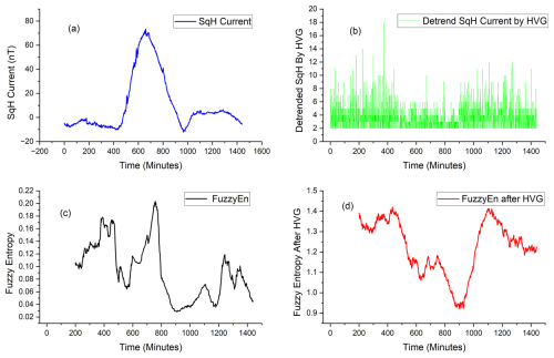

Figure 6 The sample of solar quiet current S_q(H) on 31 March 2009 at Addis Ababa, Ethiopia. (a) The time series of solar quiet current S_q(H) derived in minutes. (b) The detrended time series of the solar quiet current transformed through a horizontal visibility graph (HVG). (c) The changes in fuzzy entropy of the solar quiet current without HVG transformation. (d) The changes in fuzzy entropy of the solar quiet current with HVG transformation.

The day-to-day latitudinal distribution of entropy across the European and African sectors in January 2009 is shown in Fig. 7. The result depicts the entropy changes in color, representation. The yellow color, revealing the ranges of fuzzy entropy values between 1.2 and 1.4, indicates high entropy. This high entropy signifies the presence of ionospheric chaos in the ionospheric current system. The light-blue color ranging from approximately 0.8–1.2 reveals a declining entropy value, which indicates a transition from chaos to orderliness behavior in the ionospheric current system, while the deep-blue color ranging from 0.6–0.8 depicts low entropy values. The low entropy reveals the presence of orderliness behavior in the ionospheric current system. We noticed that in the day-to-day latitudinal distribution of entropy across the stations in the European and African sectors, some days in January 2009 depict the presence of ionospheric chaos at most of the stations, as shown in Fig. 7. High entropy values were observed at stations situated at IZN, SUA, KIV, BOX, and SOD on 1, 4, 8, 10, 14, 18–25, and 28–29 of January 2009. On 25 January, higher entropy values were depicted across all the stations in European and African sectors. This observed feature of high entropy unveils the presence of chaotic behavior in the ionospheric dynamics of the European and African sectors. Low entropy values, signifying orderliness behavior in the dynamics of ionosphere was observed on 2, 3, 5, 7, 9, 11–13, 15–16, 19–20, 23–24, 26–27, and 30–31 January. This observed low entropy is mostly domicile in the African sector. In addition, our analysis revealed that lower entropy values were found on 3, 13, and 15 January spreading across stations in the European and African sectors. This observed feature of low entropy across the European and African sectors reveals that the dynamics of the ionosphere on 13 and 15 January exhibits strong orderliness behavior.

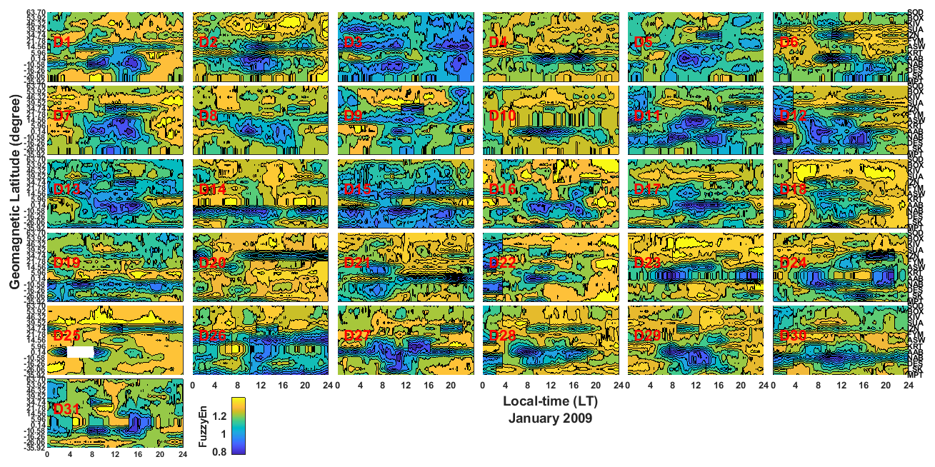
Figure 7 The day-to-day latitudinal distribution of fuzzy entropy across the European and African sectors in January 2009.

We display the contour plots of the day-to-day latitudinal distribution of entropy in February 2009 in Fig. 8. The changes in entropy depicts high values of fuzzy entropy, revealing the presence of ionospheric chaos. This trend of high entropy values was noticed on 1–2, 9–10, and 17 February, signifying that the ionospheric dynamics of the aforementioned days are associated with chaotic behavior. In addition, 1 and 17 February exhibited a higher chaotic behavior that spread across all the stations investigated. This observation further strengthens the evident influence of SSW effects on the ionospheric dynamics on these dates. Notably, low entropy implying the presence of orderliness behavior in the dynamics of the ionosphere was obvious on 4–8, 11–16, and 18–26 February 2009. However, 5 and 14 February exhibited the lowest entropy values, revealing that the state of the ionosphere exhibits strong orderliness behavior.

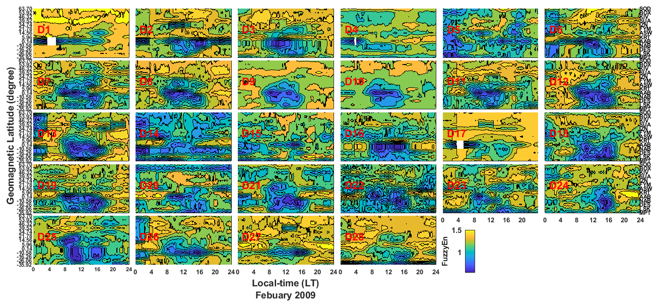
Figure 8 The day-to-day latitudinal distribution of fuzzy entropy across the European and African sectors in February 2009.

The day-to-day latitudinal distribution of entropy across the European and African sectors on March 2009 is shown in Fig. 9. Most of the fuzzy entropy values are associated with low entropy. For instance, 1–6, 8–18, 20–23, 25–28, and 31 March depict low changes in entropy at most of the stations. High entropy values associated with the presence of ionospheric chaos were found on 7 and 29–30 March.

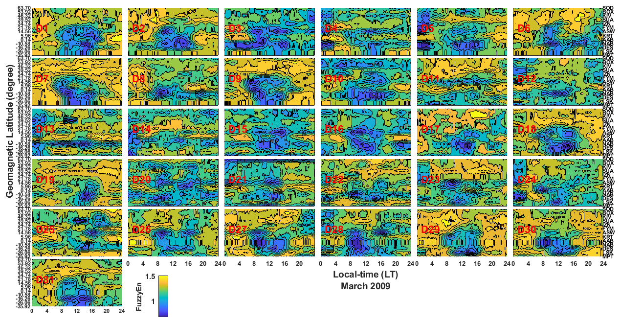
Figure 9 The day-to-day latitudinal distribution of fuzzy entropy across the European and African sectors in March 2009.

In the 2021 SSW event analysis, because of unavailability of magnetic data in the African sector, especially in stations situated within the geographical longitude of 26–40°, our analysis during 2021 SSW was restricted to only the European sector. The result of the day-to-day latitudinal distribution of entropy across the European sector is presented in Fig. 10. We observed that the changes in entropy from 1 to 6 December at the SOD, BOX, and KIV stations reveals consistently low entropy values, indicating that the state of the ionosphere at these stations exhibits consistent orderliness behavior during these periods. However, at SUA and IZN, consistent high entropy values indicating the presence of ionospheric chaos were observed from 1 to 5 December 2020. The day-to-day entropy changes on 7–9 and 11–20 December at SOD, BOX, and KIV depict a consistent high value of fuzzy entropy. Interestingly, SUA and IZN were consistently associated with a low-entropy distribution from 8 to 22 December. This observed consistent feature of low entropy at SUA and IZN signifies that the influence of SSW effects on regional ionosphere of SUA and IZN manifests an orderliness behavior in the underlying dynamics of ionosphere in this region. Furthermore, the possible emergence of ionospheric disturbances at SUA and IZN during those observed days highlights that perturbation due to 2021 SSW effect is minimal. A consistent decline feature from chaotic to orderliness behavior in the ionospheric dynamics was observed also at SOD, BOK, and KIV from 25 to 31 December 2020, while SUA and IZN exhibited some features of ionospheric chaos on 30 and 31 December.

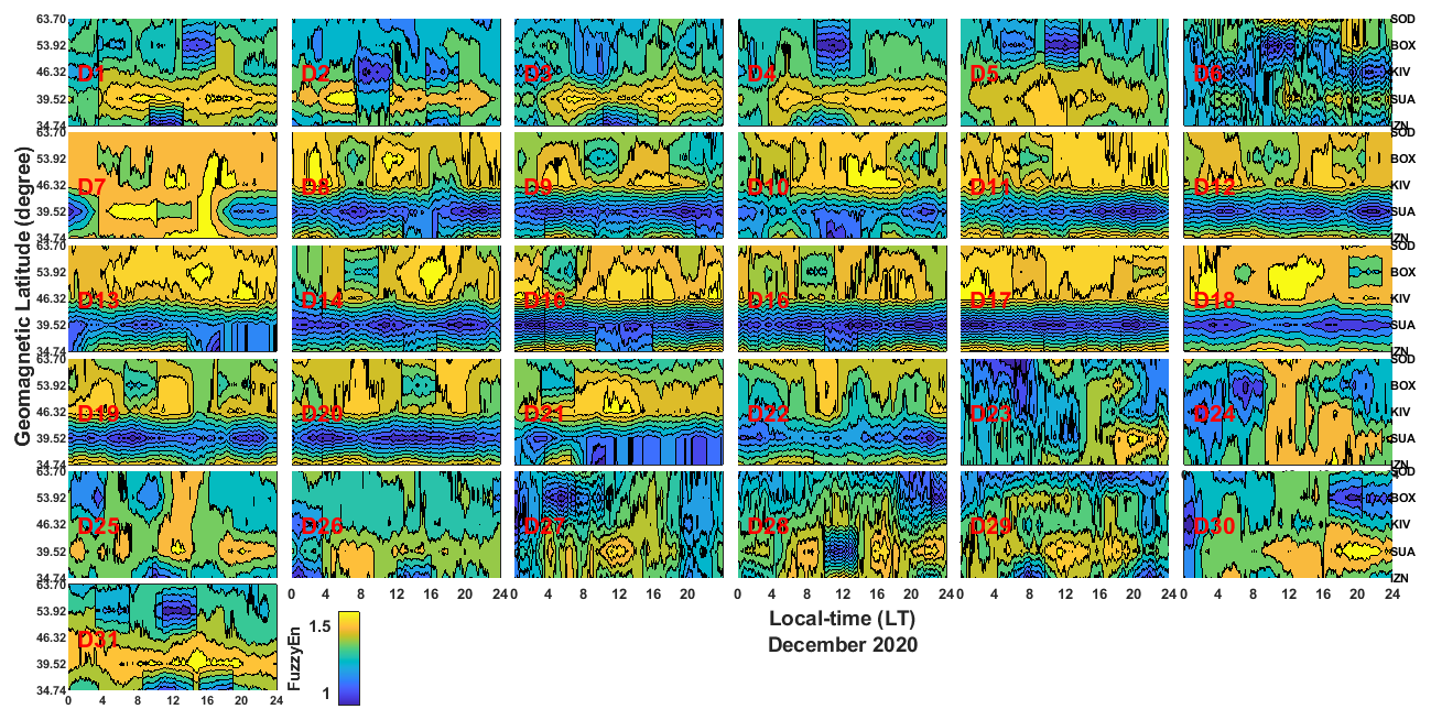
Figure 10 The day-to-day latitudinal distribution of fuzzy entropy across the European sector in December 2020.

For the SSW of January 2021, the day-to-day latitudinal distribution of entropy across the European sector is displayed in Fig. 11. The latitudinal distribution depicts low entropy across the day-to-day observation in January. For instance, 1–6, 8, 9–10, 13, 17, 19–24, 27–29, and 30–31 January reveal low entropy values across the stations investigated in the European sector, implying that the ionosphere in this region exhibits orderliness behavior in its underlying dynamics on most of the days consider in this study. Notably, high entropy, indicating the presence of ionospheric chaos, was observed at SUA and IZN on 4, 7, 10, 12, 13, and 16 January 2021. In Fig. 12, we depict the day-to-day latitudinal distribution of entropy in February 2021 across the European sector. The changes in entropy reveal high entropy, suggesting the presence of ionospheric chaos on 9, 12, 16–18, 21, and also from 24 to 27 February 2021 at SOD, BOX, SUA, and IZN. In contrast, KIV consistently exhibited low values of entropy from 1 to 8 February.

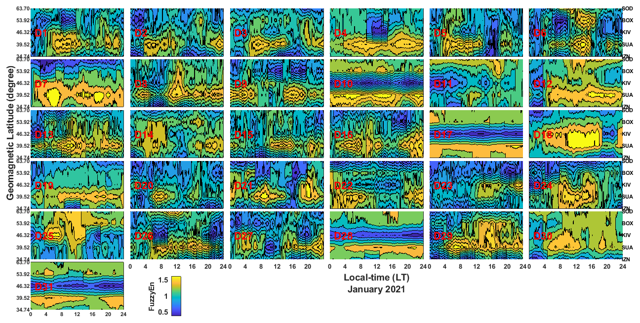
Figure 11 The day-to-day latitudinal distribution of fuzzy entropy across the European sector in January 2021.

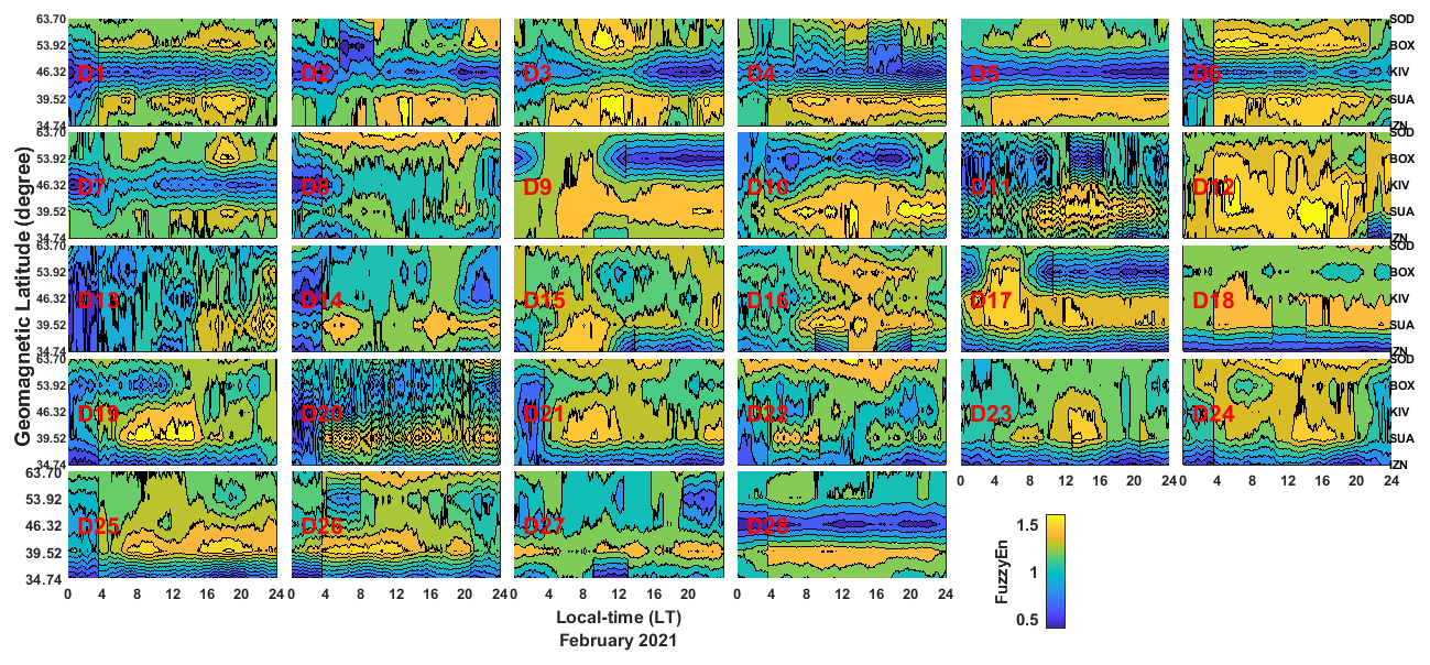
Figure 12 The day-to-day latitudinal distribution of fuzzy entropy across the European sector in February 2021.

3.1 Ionospheric chaos during phases of 2009 SSW

Displayed in Fig. 13 is the latitudinal distribution of entropy across the European and African sectors during different phases of 2009 SSW. The entropy analysis during the precondition phase of an SSW depicts high entropy values across the stations in the European sector, signifying that the precondition phase of 2009 SSW were associated with the emergence of ionospheric chaos. The observed features of high entropy values unveiling pronounced ionospheric chaos are found at SUA, KIV, BOX, and SOD. This observation further reveals that the influence of SSW effects introduces an emergence of ionospheric perturbation in SUA, KIV, BOX, and SOD at the preconditioning phase of the 2009 SSW in the European sector. It is noteworthy that the period from January to March 2009 was strongly associated with minimal activities of geomagnetic disturbance (see Fig. 2a). In the African sector, we noticed that the SSW preconditioning phase is characterized by declining and low entropy values, implying that the regional ionosphere across the African sector reveals a suppression of orderliness behavior in the ionospheric dynamics in the preconditioning phase of the 2009 SSW. Low entropy was seen at AAB, NAB, and DES during the preconditioning phase, signifying that the underlying dynamics of the ionosphere at AAB, NAB, and DES are exhibiting orderliness behavior as the preconditioning phase of the SSW emerges.

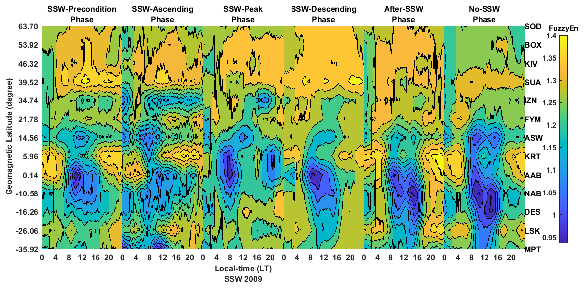
Figure 13 The latitudinal distribution of fuzzy entropy across the European and African sectors during the phases of 2009 SSW.

During the ascending phase of the SSW, we observed also low entropy values at stations in the African sector up to IZN. However, high values of entropy implying the presence of ionospheric chaos were noticed at KIV, BOX, and SOD. The high entropy observed at KIV, BOX, and SOD during the ascending phase signifies that the influence of the SSW effect on the regional ionosphere at KIV, BOX, and SOD is imminent. This suggests that SSW events significantly affect ionospheric dynamics, leading to an increased chaotic pattern across the European sector during the ascending phase of the 2009 SSW. In the African sector, we observed that the region depicts low entropy values during the ascending phase. This further signifies that the regional ionosphere in the African sector demonstrates orderliness behavior in the ascending phase of an SSW.

During the peak phase of SSW 2009, evidence of ionospheric chaos was obvious at SOD, BOX, KIV, and SUA. The changes in fuzzy entropy during this peak phase depicts high values, indicating significant disturbances in the ionosphere in the European sector. The feature of a declining entropy value was noticed to have spread from IZN to DES. However, at around 04:00–10:00 LT, low entropy values were seen at KRT, AAB, and NAB. This observed declining entropy with a brief feature of low entropy at KRT, AAB, and NAB reveals that the regional ionosphere in the African sector during the peak phase of the SSW experiences a suppression of orderliness behavior. The suppression of orderliness behavior as SSW peak phases emerges further, suggesting that the regional ionosphere of the African sector also experiences chaotic behavior. However, the European sector during the peak phase depicts a higher degree of chaotic behavior. We suspect that the emergence of chaotic behavior due to the SSW effect in the African sector results in the suppression of orderliness behavior.

At the descending phase of an SSW, high entropy values associated with the presence of ionospheric chaos were evident at SOD, BOX, KIV, SUA, and IZN. However, FYM, ASW, KRT, DES, LSK, and MPT reveal a declining entropy value, while AAB and NAB at around 08:00–16:00 LT of the descending phase of the SSW depict low entropy values. The observed feature of declining entropy during the descending phase at stations situated in the African sector signifies that the ionospheric dynamics exhibits a suppression in orderliness behavior. This suppression of orderliness further suggests that the SSW effects during the descending phase introduce perturbation into the regional ionosphere of Africa, resulting in the suppression of orderliness behavior.

The after-SSW phase of 2009 also demonstrates a distribution of high values of entropy at SOD, BOX, KIV, SUA, SUA, and FYM. In the stations situated in the African sector, low entropy begins to spreads from AAB to LSK, while ASW, KRT, and MPT depict a declining value of entropy. The observed entropy changes during the after-SSW phase signify that the SSW-induced effect on African regional ionosphere begins to decline. During the no-SSW phase, the degree of entropy associated with ionospheric chaos is suppressed at the following stations: SOD, BOX, KIV, SUA, and IZN, while a steady low entropy value was seen around ASW, KRT, AAB, NAB, DES, LSK, and MPT stations. These steady low entropy features seen during the no-SSW phase reveal that the regional ionosphere of the African sector recovers back to its original dynamics.

3.2 Ionospheric chaos during phases of 2021 SSW

Shown in Fig. 14 is the 2021 SSW latitudinal distribution of entropy across the European sector at precondition, ascending, peak, descending, after-SSW, and no-SSW phases. The precondition phase at SOD, BOX, and KIV depicts high values of entropy signifying that ionospheric chaos is dominant during this period, while a declining and low entropy change was observed at IZN and SUA. The ascending, peak, descending, and after-SSW phases exhibit a consistent low entropy value in their latitudinal distribution, suggesting orderliness behavior in the ionosphere at SOD, BOX, and KIV. In contrast, at SUA, a consistent increase in entropy was evident. This consistent increase in entropy at SUA during all the phases of the SSW implies that the ionospheric dynamics are consistently exhibiting chaotic behavior due to the influence of the SSW.

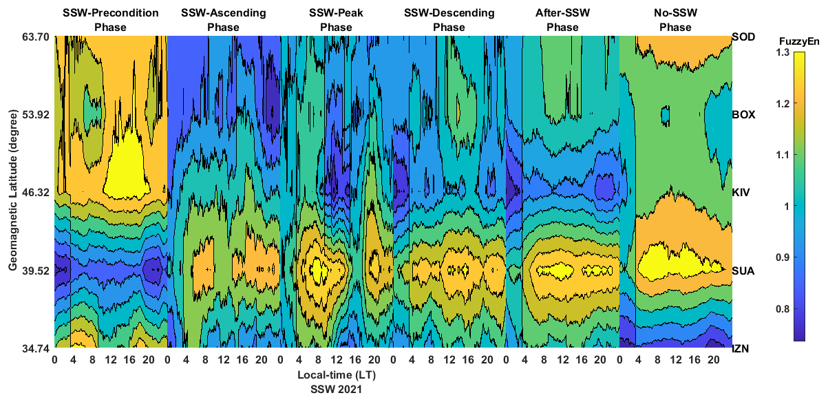
Figure 14 The latitudinal distribution of fuzzy entropy across the European sector during the phases of 2021 SSW.

4 Discussion of results

The results unveil the dynamical characteristics in the solar quiet current, S_q(H), system during the 2009 and 2021 SSW events. Employing the horizontal visibility graph (HVG) and fuzzy entropy analysis, this study quantifies the chaotic and orderliness behavior exhibited by the ionospheric current system during SSW events across the European and African sectors. Ionospheric chaos is found to be most pronounced at European sector stations, particularly at SUA, KIV, BOX, and SOD, demonstrating a higher degree of complexity and unpredictability in the ionospheric dynamics at these locations. A notable dynamical feature of the ionospheric current system within the African sector was the consistent low entropy values observed at AAB, NAB, and DES, indicating the presence of orderliness behavior. In addition, our analysis revealed a transition from chaotic to orderliness behavior in the African sector as the stratospheric warming intensified. This transition was accompanied by a decline in entropy values. For instance, during the preconditioning phase of the 2009 SSW, our results showed a decline in entropy values, signifying a shift towards orderliness behavior. Specifically, FYM, ASW, KRT, DES, LSK, and MPT exhibited declining entropy values, while AAB and NAB showed low entropy values around 09:00–11:00 LT. This decline in entropy during the preconditioning phase suggests that the SSW effects introduce perturbation to the regional ionosphere of the African sector, leading to a suppression of chaotic behavior and transit to orderliness behavior in the African sector. The European sector stations, comprising SOD, BOX, KIV, SUA, and IZN, exhibited elevated entropy values, signifying the presence of pronounced ionospheric chaos in the preconditioning phase. During the ascending phase of the 2009 SSW, our analysis revealed that the European sector stations (SOD, BOX, KIV, SUA, and IZN) consistently exhibited high entropy values, indicating the presence of chaotic behavior. This pronounced ionospheric chaos suggests that the SSW-induced effects on the regional ionosphere of the European sector are particularly significant. By comparison, the African sector exhibited more variable entropy measures, fluctuating between declining and low entropy values. Notably, African stations, comprised of FYM, ASW, KRT, AAB, NAB, DES, LSK, and MPT, showed low entropy values between 08:00 and 12:00 LT, while declining entropy values were observed at other local times. This divergence suggests that the ionosphere in the African sector is becoming more synchronized to orderliness behavior as the stratospheric temperature rises.

At the peak phase of the 2009 SSW, our findings reveal an extended feature of converging orderliness behavior in the African sector. Notably, declining entropy values were observed at FYM, ASW, KRT, DES, LSK, and MPT, while low entropy values were evident at AAB and NAB. This converging orderliness behavior in the African sector during the SSW peak phase suggests that an external perturbation, induced by SSW effects, is influencing the regional ionosphere. This perturbation appears to suppress the chaotic behavior of the ionospheric current system in the African sector. Meanwhile, stations in the European sector, including SOD, BOX, KIV, and SUA, continued to exhibit chaotic behavior in their regional ionospheric dynamics. The descending phase of the 2009 SSW reveals a gradual recovery to orderliness behavior in the African sector. Low entropy values were evident, indicating a return to orderliness dynamics in the regional ionosphere. The recovery was characterized by low entropy values at KRT, AAB, NAB, and DES, while other African sector stations exhibited declining entropy values. This observed entropy distribution during the SSW's descending phase suggests that the African sector's regional ionosphere is reverting to orderliness behavior. Conversely, European sector stations, including IZN, SUA, KIV, BOX, and SOD, consistently displayed chaotic behavior.

During the after-SSW phase, a notable decline in entropy was observed at FYM, ASW, KRT, LSK, and MPT, implying a transition towards orderliness behavior at these stations. Additionally, low entropy values were recorded from AAB to DES, signifying that the ionosphere at AAB, NAB, and DES exhibited orderliness behavior. On the other hand, the European sector, including SOD, BOX, KIV, SUA, and IZN, continued to exhibit high entropy values suggesting a persistent ionospheric chaos. At the no-SSW phase, a notable expansion and spread of low entropy values were observed across all stations in the African sector. This entropy distribution pattern indicates that the regional ionosphere has fully recovered and the dynamics have reverted to orderliness behavior.

In the 2021 SSW, entropy analysis revealed distinct patterns of ionospheric chaos and orderliness across different stations. Initially, chaos increased at KIV, BOX, and SOD during the preconditioning phase, while SUA and IZN exhibited orderly behavior. In contrast, SOD, BOX, and KIV showed orderly behavior during the ascending, peak, and descending phases. However, chaos re-emerged at these stations during the after-SSW and no-SSW phases. Notably, SUA exhibited prominent chaotic behavior throughout the ascending, peak, descending, after, and no-SSW phases, highlighting the significant influence of an SSW on ionospheric dynamics in certain regions of the European sector.

These findings of ionospheric chaos in most of the stations situated in the European sector reveal the evidence of the fact that the 2009 SSW effect indeed significantly influenced the ionospheric dynamics in the European sector. Interestingly, during the 2009 SSW periods, the daily geomagnetic activities were mostly characterized by a planetary index of K_p≤3. However, we notice some certain days during the SSW periods – namely, SSW 2009 (3, 19, and 26 January; 4, 14–15, 25, and 28 February; and 13 and 24 March) and SSW 2021 (10, 21, and 23 December; 5, 6, 11, 24, 25, and 27 January; 2, 6, 12, 16, 20, 22, and 23 February) – where there was a transient increase in the K_p values exceeding 3 within the 3 h intervals of the K_p index. Notably, these transient emergence of K_p index exceeding 3 within a few hours during SSW periods have a tendency of inducing a mild geomagnetic disturbance during the SSW period but may not be strong enough to be a dominant factor to influence ionospheric instability during SSW. The reason is that SSW events occur on a longer timescale, i.e., number of days, compared to the emergence of sudden geomagnetic disturbance within a few hours. The contributing influence of an SSW is more significant than the transient disturbance of geomagnetic activities, while we acknowledge that there is some transient geomagnetic disturbance revealed by the K_p index during SSW periods. To address these possible geomagnetic disturbances indicated by the K_p index and all our daily solar quiet current derivation analysis during the SSW periods, we implement the subtraction of the geomagnetic storm index in minutes (SYM-H) from the H component of the magnetic field to minimize the influence of geomagnetic disturbances. Therefore, the finding that ionospheric chaos is dominant in most stations located in the European sector provides additional evidence of the SSW's effect on the regional ionosphere in European sector. The presence of ionospheric chaos unveils the formation of large disturbances in the European sector owing to the impact of disruption on communication and navigation signals during SSW. We suspect that this observation of ionospheric chaos may be attributed to the enhancement of the solar and lunar migrating tides during SSWs, which influence the generation of electric fields through the E-region dynamo mechanism (Goncharenko et al., 2021; Pedatella et al., 2014; Siddiqui et al., 2018). Another contributing factor to the emergence of ionospheric chaos could be the heliospheric plasma sheet's interaction with the Earth's magnetosphere, which lead to significant magnetospheric processes like relativistic electron dropout (RED) and EMIC wave generation. These processes have downstream effects on the lower atmospheric activities, potentially influencing the weather pattern and climate through energy deposition and ionization changes (Tsurutani et al., 2016; Salminen et al., 2020).

The latitudinal distribution of entropy showed a transition from chaotic to orderliness behavior in the African sector during the peak, descending, and after-SSW phases, highlighting the impact of SSW on the regional ionosphere of the African sector, which leads to the suppression of orderliness behavior. This observed orderliness behavior in the African sector's ionosphere cannot be attributed to the equatorial electrojet (EEJ) because EEJ is typically confined to the magnetic equation (±3°). The result of our analysis reveals that the observed orderliness behavior extends beyond the equatorial boundary. We suspect that the observed suppression and consistency in orderliness behavior reflects that there is modification in the equatorial ionization anomaly (EIA) structure of the African sector due to the forcing effect from SSW and other external sources like the heliospheric plasma sheet (HPS), magnetospheric processes (REDs, EMIC waves, etc.), and their impacts on the lower atmosphere (via disturbance chains). The extension of orderliness behavior, associated with low entropy values, spans from Addis Ababa (AAB) to Fayum (FYM) and Maputo (MPT), indicating a significant alteration in the EIA structure driven by SSW influences. In our forthcoming research, we focus extensively on this orderliness behavior within the ionospheric current system, particularly in the African equatorial region.

5 Conclusion

This study unveils the contributing influence of SSWs on the regional ionosphere across Europe and Africa by examining ionospheric chaos in the solar quiet current during the SSW events of 2009 and 2021. These SSW events occurred during the solar minimum years of solar cycle 24. The SSW was categorized according to the rising stratospheric temperature into six phases – namely, precondition, ascending, peak, descending, after-, and no-SSW phases. The study covers 13 magnetometer stations across the European and African sectors located within the geographical longitude of 26 to 40° E. Magnetometer data obtained during the periods of SSW were used to derive the time series of the solar quiet current, S_q(H). These solar quiet current time series were transformed into a network representation through the horizontal visibility graph (HVG) approach and analyzed by fuzzy entropy to quantify the presence of ionospheric chaos during the periods of SSW. We found that the latitudinal distribution of entropy depicts high entropy, indicating the presence of ionospheric chaos in most of the stations situated within the European sector compared to stations in the African sector. A consistent low-entropy distribution unveiling the presence of orderliness behavior was found to be prominent in the African sector. This prevailing evidence of orderliness behavior in the African sector during SSW signifies that the contribution influence of the SSW to the regional ionosphere of the African sector manifests an orderliness behavior in its underlying dynamics. While the pronounced features of ionospheric chaos associated with high entropy values were found in the European sector. This ionospheric chaos unveils the evidence of significant effects of SSWs on the regional ionosphere in Europe. Finally, we found that after the peak phase of an SSW, the ionospheric chaos is more pronounced.