Multifractality of climate networks

Geophysical fields are extremely variable over a wide range of space–time scales. More specifically, they are intermittent in the sense that the strongest fluctuations are increasingly concentrated in sparser and sparser fractions of the space–time domain. Multifractals have been developed to analyze and simulate intermittency across scales, while climate networks can detect and characterize extreme-event synchronization. In contrast to multifractal analysis, climate networks are usually generated at a given observation scale despite displaying complex structures over larger scales and being likely to exhibit similar complexity at smaller scales.

In this letter, we present how to overcome this dichotomy of approaches by analyzing in detail the effects of increasing the observation scale for climate networks as allowed by empirical data; i.e., how do they upscale? This must be understood as a preliminary step to be able to downscale them, including for practical applications such as urban geosciences that require the analysis and simulation of intermittent fields at a very high resolution. This is one of the reasons why we are using precipitation to illustrate our multifractal climate network approach.

1 Introduction

Climate networks (Tsonis and Roebber, 2004; Donges et al., 2009) have been extensively used to study long-range dependence and/or synchronization (teleconnections) between the different spatial locations of various geophysical fields using different statistical methods such as cross-correlation (Tsonis and Roebber, 2004; Donges et al., 2009), event synchronization (Malik et al., 2012; Boers et al., 2019), and mutual information (Hlinka et al., 2013; Donges et al., 2009). However, geophysical processes are highly intermittent and vary in terms of intensity, emerging from complex nonlinear interactions across different space–time scales. Networks are typically constructed at the available data resolution and do not account for possible inter- and/or intra-scale interactions. Recent advances in this direction have combined a wavelet-based approach to tentatively account for synchronizations at different temporal scales (Agarwal et al., 2017; Kurths et al., 2019). In contrast, multifractals (Schertzer and Lovejoy, 1987; Schertzer et al., 1997; Schertzer and Lovejoy, 1991; Lovejoy et al., 2010) provide a natural framework to analyze and simulate extremely varying and intermittent geophysical and environmental fields over various scales. The core idea is to regard these complex systems as a cascade of structures (Richardson, 1922; Yaglom, 1966; Mandelbrot, 1974) across a wide range of scales, thus generating long-range nonlinear interactions between them. Here, we propose a substantial extension of the climate network approach to multiple scales in a systematic way, accounting for the intermittency and anisotropy in space and time as highlighted by multifractals, which are able to capture the dynamical behaviors of long-range interactions.

2 Data and methods

Although our multifractal climate network approach is quite general, we will introduce it and illustrate it with the Tropical Rainfall Measuring Mission (TRMM) satellite and the gauge-combined gridded precipitation dataset 3B42-v7 (Huffman et al., 2007, 2016). Specifically, a subset of the dataset over the South Asian subcontinent (3.875–38.875° N, 63.125–97.125° E) is used to analyze the extensively researched Indian summer monsoon (ISM), which is large enough to include some range of teleconnections while remaining computationally feasible. Data were sampled from June to September (122 d), which are typically associated with monsoon activity, for the total available time period of 22 years (1998–2019). The selected dataset has a high spatial resolution of 0.25° × 0.25° (roughly 20 000 grid points), and daily aggregates of 3 h high-resolution data are used to avoid the effects of synchronization and/or dependence on networks as induced by the diurnal cycle.

2.1 Multifractal analysis of precipitation

Cascades and multifractals originate from turbulence and physically correspond to the concentration of the turbulent energy flux along the cascade within smaller and smaller fractions of the space–time embedding space. The large multiplicity of interactions can generate universal properties, which are defined by only a few relevant parameters that are, furthermore, physically meaningful (Schertzer and Lovejoy, 1987; Schertzer et al., 1997). The resulting universal multifractal (UM) framework has often been used to analyze the precipitation component of the weather and climate (Lovejoy and Schertzer, 2013). In order to analyze the rain rate R, the data are systematically coarse-grained in space and/or time to decrease the resolution. Let L denote the largest scale, and let ℓ denote the degraded resolution; then, the scale ratio $\mathit{\lambda }=L/\mathrm{\ell }$ is the (dimensionless) resolution. The scale ratios in space and time can be denoted separately by, respectively, λ_s and λ_t when both are degraded to different resolutions. They are related by ${\mathit{\lambda }}_{\mathrm{t}}\approx {{\mathit{\lambda }}_{\mathrm{s}}}^{\mathrm{2}/\mathrm{3}}$ to account for the anisotropy between horizontal space and time (Schertzer and Lovejoy, 1987, 1989, 1991), and this is typically applied to 2D+1 space–time fields.

Let φ_λ be the underlying cascading field conserved at all scales; i.e 〈φ_λ〉=constant. Then the scaling parameter H characterizes the deviation of the rain rate R_λ (at resolution λ) from conservation:

$$\begin{array}{}\text{(1)}& \mathrm{\Delta }{R}_{\mathit{\lambda }}\approx {\mathit{\phi }}_{\mathit{\lambda }}{\mathit{\lambda }}^{-H}\Rightarrow \langle \left|\mathrm{\Delta }{R}_{\mathit{\lambda }}\right|\rangle \approx {\mathit{\lambda }}^{-H},\end{array}$$

where the sign ≈ denotes an asymptotic equivalence for large resolutions (λ≫1), i.e., with prefactors ≠1 and possibly being coupled with an equality in the probability distribution when random variables are involved. The normalized moments of φ_λ scale with the moment scaling exponent K(q):

$$\begin{array}{}\text{(2)}& {\displaystyle \frac{\langle {\mathit{\phi }}_{\mathit{\lambda }}^q\rangle }{\langle {\mathit{\phi }}_{\mathrm{1}}{\rangle }^q}}={\mathit{\lambda }}^{K\left(q\right)}.\end{array}$$

Similarly, the exceedance probability distribution of φ_λ scales with the codimension function c(γ):

$$\begin{array}{}\text{(3)}& \mathrm{Pr}\left({\displaystyle \frac{{\mathit{\phi }}_{\mathit{\lambda }}}{\langle {\mathit{\phi }}_{\mathit{\lambda }}\rangle }}\ge {\mathit{\lambda }}^{\mathit{\gamma }}\right)\approx {\mathit{\lambda }}^{-c\left(\mathit{\gamma }\right)},\end{array}$$

where $\mathit{\gamma }=\log ({\mathit{\phi }}_{\mathit{\lambda }}/\langle {\mathit{\phi }}_{\mathit{\lambda }}\rangle )/\log \mathit{\lambda }$ is the scale-invariant singularity. Both the moment and probability exponent functions are related by means of the following Legendre transforms (Parisi and Frisch, 1985):

$$\begin{array}{}\text{(4)}& K\left(q\right)=\underset{\mathit{\gamma }}{max}(q\mathit{\gamma }-c(\mathit{\gamma }\left)\right),c\left(\mathit{\gamma }\right)=\underset{q}{max}(q\mathit{\gamma }-K(q\left)\right).\end{array}$$

Under the UM framework, both K(q) and c(γ) of conservative multifractal fields depend only on the parameters α and C₁:

$$\begin{array}{}\text{(5)}& {\displaystyle }K\left(q\right)& {\displaystyle }=\left\{\begin{array}{ll}\frac{C_{\mathrm{1}}}{\mathit{\alpha }-\mathrm{1}}(q^{\mathit{\alpha }}-q),& \mathit{\alpha }\ne \mathrm{1}\\ C_{\mathrm{1}}q\log \left(q\right),& \mathit{\alpha }=\mathrm{1}\end{array}\right.,\text{(6)}& {\displaystyle }c\left(\mathit{\gamma }\right)& {\displaystyle }=\left\{\begin{array}{ll}{C}_{\mathrm{1}}{\left(\frac{\mathit{\gamma }}{C_{\mathrm{1}}{\mathit{\alpha }}^{\prime }}+\frac{\mathrm{1}}{\mathit{\alpha }}\right)}^{{\mathit{\alpha }}^{\prime }},& \mathit{\alpha }\ne \mathrm{1}(\text{with }\mathrm{1}/\mathit{\alpha }+\mathrm{1}/{\mathit{\alpha }}^{\prime }=\mathrm{1})\\ C_{\mathrm{1}}\exp \left(\frac{\mathit{\gamma }}{C_{\mathrm{1}}}-\mathrm{1}\right),& \mathit{\alpha }=\mathrm{1}\end{array}\right.,\end{array}$$

where $\mathrm{0}\le \mathit{\alpha }\le \mathrm{2}$ measures the degree of multifractality, with α=0 for monofractal fields and α>1 for the class of multifractal processes having unbound extreme singularities, and $\mathrm{0}\le C_{\mathrm{1}}\le d$ is the codimension of the mean field (d is the dimension of the embedding space). Figure 1 plots the estimated K(q) curve using single trace moments (TM) (Schertzer and Lovejoy, 1987; Lavallée et al., 1992) of the conserved field at different scales in space and time (see Eq. 2). Equation (5) then yields the values of α and C₁ from K(q). H can be estimated similarly using the first-order structure function (see Eq. 1) and also using the relation $\mathit{\beta }=\mathrm{2}H+\mathrm{1}-K\left(\mathrm{2}\right)$ between the spectral exponent β and the second-order moment exponent K(2), as shown in Fig. 1.

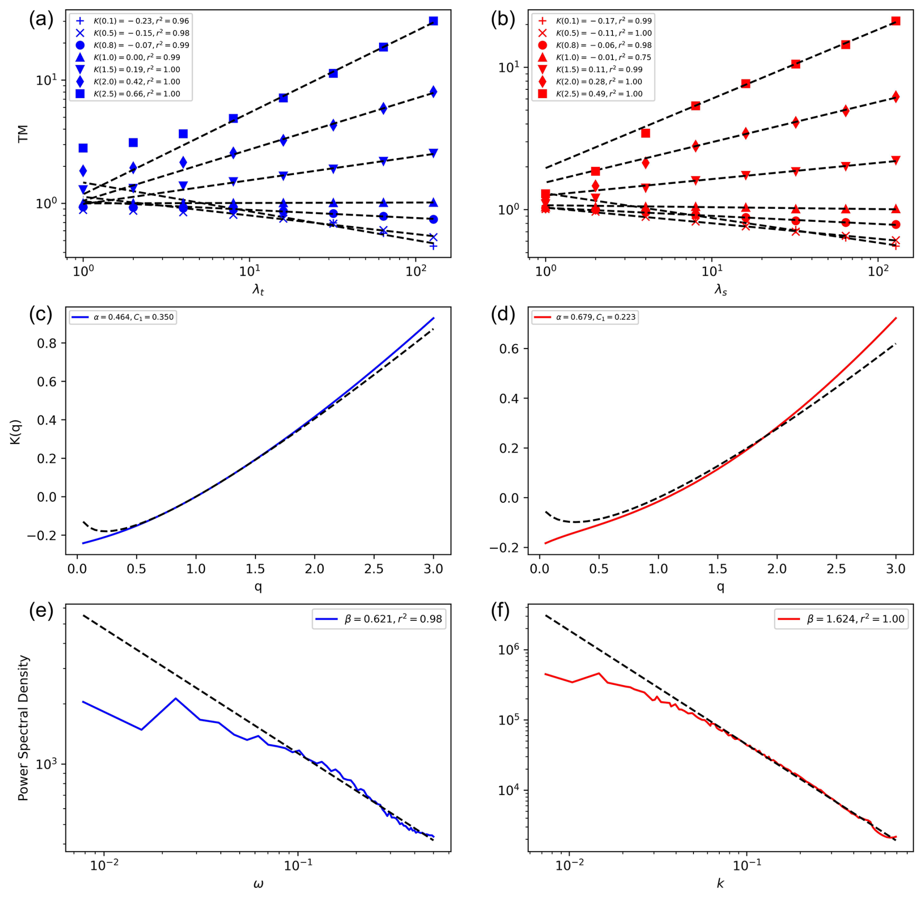
Figure 1 A set of graphs computing the UM parameters for time and space in the left and right columns, respectively. Trace moment (TM) plots are shown in the first row, with scale break at 440 km in space and 16 d in time. The second row plots the moment-scaling exponent K(q) obtained from the TM in the first row. Parameters α and C₁ calculated from K(q) are also shown, along with the corresponding theoretical K(q) curves (dotted line). Power spectra shown in the third row, used to estimate H from the spectral slope β, also indicate the deviation in scaling around 460 km in space and 10 d in time. The break around 16 d can be attributed to the synoptic maximum in time. On the other hand, the break around 440–460 km is difficult to explain but could be attributed to the spatial scale of the synoptic Indian summer monsoon (ISM) activity (estimated in Malik et al., 2012) since it disappears when samples from the whole year are analyzed.

2.2 Precipitation climate networks using time-delayed mutual information

Climate networks are constructed between time series R_i and R_j at different geographical locations called nodes or vertices ($i,j\in V$) by connecting pairs of them with links (denoted i∼j) if a given measure of similarity $\mathbf{S}(R_i,R_j)\ge \mathrm{0}$ of the pair is significant. Unweighted CNs can be constructed from the strongest similarities by thresholding the similarity matrix S:

$$\begin{array}{}\text{(7)}& A_{i,j}=\mathrm{\Theta }(S_{i,j}-\mathit{\theta })-{\mathit{\delta }}_{i,j}=\left\{\begin{array}{ll}\mathrm{1},& S_{i,j}\ge \mathit{\theta },i\ne j\\ \mathrm{0},& \text{otherwise}\end{array}\right.,\end{array}$$

where A is used to denote the adjacency matrix of a network, θ is some threshold of S, δ(x) is the Kronecker delta to remove self-links i∼i, and Θ(x) is the Heaviside function. The links of a network can be directed, possibly implying a direction of causality between two connected time series. However, we will be focusing on undirected networks here and, consequently, on symmetric similarity and adjacency matrices. Network centrality measures such as the degree (${\text{deg}}_i={\sum }_j{A}_{i,j}$), which gives the number of links connecting a given node, are used to study a network's properties.

Time-delayed mutual information (TDMI) (Hlaváčková-Schindler et al., 2007; Hlinka et al., 2013; Haas et al., 2023) has been used here to estimate the general dependence between two time series. Let R_λ(x,t) denote precipitation time series at the position vector x, time t, and resolution λ; then, TDMI is calculated as follows:

$$\begin{array}{}\text{(8)}& \begin{array}{rl}& I\left(R_{\mathit{\lambda }}(\mathit{x},t),R_{\mathit{\lambda }}(\mathit{y},t+\mathit{\tau })\right)=\iint p\left(R_{\mathit{\lambda }}(\mathit{x},t),R_{\mathit{\lambda }}(\mathit{y},t+\mathit{\tau })\right)\\ & \log \left({\displaystyle \frac{p\left(R_{\mathit{\lambda }}(\mathit{x},t),R_{\mathit{\lambda }}(\mathit{y},t+\mathit{\tau })\right)}{p\left(R_{\mathit{\lambda }}(\mathit{x},t)\right)p\left(R_{\mathit{\lambda }}(\mathit{y},t+\mathit{\tau })\right)}}\right)\\ & \mathrm{d}{R}_{\mathit{\lambda }}(\mathit{x},t)\mathrm{d}{R}_{\mathit{\lambda }}(\mathit{y},t+\mathit{\tau }),\end{array}\end{array}$$

where p(R_λ(x,t)) and $p\left(R_{\mathit{\lambda }}(\mathit{x},t)R_{\mathit{\lambda }}(\mathit{y},t+\mathit{\tau })\right)$ are the marginal and joint distributions, respectively. TDMI can also be used by thresholding the rain to account for the dependence between extreme rain events. The TDMI-based similarities between two time series R_λ(x,t) and $R_{\mathit{\lambda }}(\mathit{y},t+\mathit{\tau })$ are then given by

$$\begin{array}{}\text{(9)}& \begin{array}{rl}{\mathbf{S}}_{\mathit{\lambda }}(\mathit{x},\mathit{y})& ={\displaystyle \frac{I_{\mathit{\lambda }}(\mathit{x},\mathit{y})}{max\left(I_{\mathit{\lambda }}(\mathit{x},\mathit{x}),I_{\mathit{\lambda }}(\mathit{y},\mathit{y})\right)}},\text{ where }{I}_{\mathit{\lambda }}(\mathit{x},\mathit{y})\\ & =\underset{\mathit{\delta }(\mathit{x},\mathit{y})<\mathit{\tau }\le {\mathit{\tau }}_{\mathit{\lambda }}}{max}I\left(R_{\mathit{\lambda }}(\mathit{x},t),R_{\mathit{\lambda }}(\mathit{y},t+\mathit{\tau })\right).\end{array}\end{array}$$

The delay at which the dependence is maximized between two time series is called the correlation delay (τ(x,y)), which is a function of the position vectors. A maximal delay τ_λ is set while computing the similarity between any two pairs of time series to limit the creation of false links from unreasonably large τ(x,y). The denominator proposed above acts as a normalizing factor which accounts for the self-information (auto-correlation) between time series. More detailed information on the TDMI properties and its implementation can be found in the Supplement.

3 Climate networks at multiple scales

3.1 Coarse-field networks (CFNs)

As pointed out in the Introduction, the change of scale for CNs can have at least two meanings:

• i.

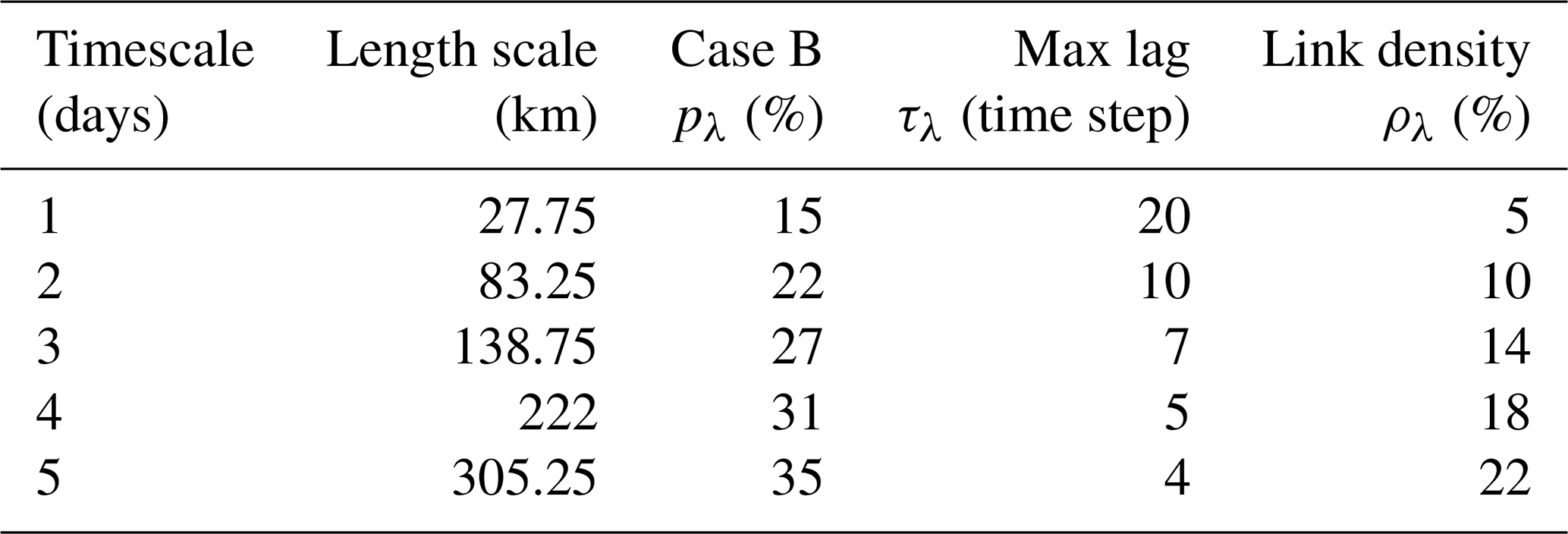
  It can correspond to coarse graining of the rainfall data in space and time using the scale ratios from Sect. 2.1 and the obtainment of networks at various larger scales, calculated in this letter for up to five different scales (see Table 1).

• ii.

  This can also be done the other way around, i.e., computing the climate network at a given scale and then degrading its resolution.

Multifractal climate networks (MCNs) will be used to denote both these definitions. In this subsection, we proceed with the first definition of MCNs, called coarse-field networks (CFNs). They are constructed over a range of scales where the UM parameters remain unchanged (up to the scale break in Fig. 1) and are parameterized by p_λ,θ_λ, and τ_λ, which depend on the data resolution λ.

TDMI-based CFNs are constructed here for two case scenarios: (A) using similarity measures from the whole range of precipitation values and (B) using extreme precipitation events above a certain threshold rainfall value (in fact, a fixed singularity γ). The threshold rain value required for case B can be calculated from the multifractal relation in Eq. (3):

$$\begin{array}{}\text{(10)}& p_{\mathit{\lambda }}=\mathrm{Pr}\left(R_{\mathit{\lambda }}\ge {\mathit{\lambda }}^{\mathit{\gamma }}\right)\approx {\mathit{\lambda }}^{-c\left(\mathit{\gamma }\right)}.\end{array}$$

The corresponding parameter p_λ, which only applies to case B since case A does not require thresholding, was fixed at the largest resolution (p_Λ=0.15) and calculated for the rest of the scales using Eq. (10) by keeping constant the singularity γ (see Table 1 for p_λ values).

Table 1 MCN parameter values used for the computation of CNs at five different scales are shown below. The p_λ values for case A are omitted from this table since case A would equate to taking the complete range of rainfall values for each scale. Length scales in the second column correspond to grid lengths at the Equator.

The adjacency matrix A is obtained by thresholding the similarity matrix S_λ with some threshold parameter θ_λ (see Eq. (7)). This θ_λ directly influences the network structure and its properties, such as degree, link distribution, and clustering coefficient, by controlling the density of links, denoted by ρ_λ. If S_λ is assumed to be a multifractal measure then an equation similar to Eq. (10) is obtained, relating ρ_λ at different scales to the threshold singularity γ_S:

$$\begin{array}{}\text{(11)}& {\mathit{\rho }}_{\mathit{\lambda }}=\mathrm{Pr}\left({\mathbf{S}}_{\mathit{\lambda }}\ge {\mathit{\theta }}_{\mathit{\lambda }}\right)={\mathit{\lambda }}^{-c_S\left({\mathit{\gamma }}_S\right)};{\mathit{\theta }}_{\mathit{\lambda }}={\mathit{\lambda }}^{{\mathit{\gamma }}_S}.\end{array}$$

Finally, the τ_λ free parameter sets the maximal delay (lag) up to which the strength of dependence between two given time series is calculated. This maximal correlation timescale is usually significantly larger than the average lifetime of rain events at a given resolution, which makes it difficult to estimate at different scales. The CFN computations for τ_Λ>40 d were found to significantly change the spatial pattern of node degrees, whereas the results remained consistent when varied between 6 and 20 d. Therefore, τ_Λ was fixed to 20 d at scale Λ. For λ<Λ, τ_λ is lowered to keep the effective maximal delay at all scales nearly constant at 20 d; i.e., ${\mathit{\tau }}_{\mathit{\lambda }}={\mathit{\tau }}_{\mathrm{\Lambda }}{\mathit{\lambda }}_{\mathrm{t}}^{-\mathrm{1}}$ (see Table 1).

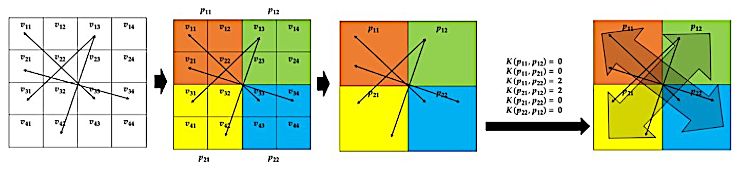
Figure 2 Scaled climate network (SCN) schematic: smaller nodes are grouped together, shown here in different colors, with linked nodes being replaced by linked groups. The grouping of the node set directly corresponds to the upscaling of the field in space.

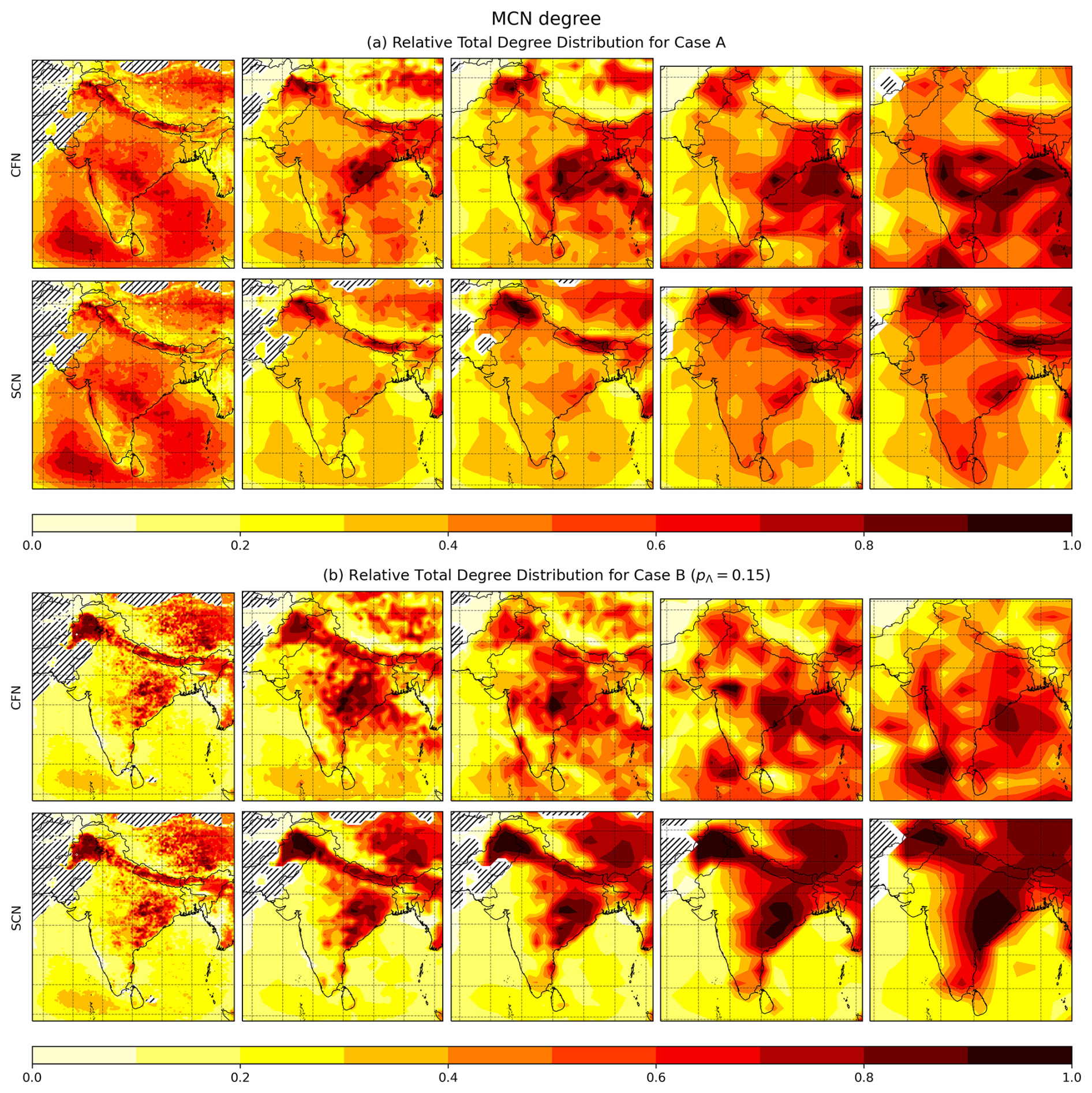
Figure 3 Relative degrees for both approaches, namely coarse-field networks (CFNs, top row) and scaled climate networks (SCNs) (bottom row), at different scales λ are plotted for two cases. (a) Case A: full range of the rain rate. (b) Case B: p_Λ=0.15 thresholded time series (see Table 1 for all parameter values). The resolution in space decreases from left to right. The distribution of CFN hubs (high-degree nodes) in space differs significantly with decreasing resolution compared to the SCN hubs, which are more stable and appear to be independent of it and are more prominent in (b). The dashed regions were not included in the analysis due to a lack of samples as a result of scanty rainfall (< 15 % rainy days during the period of study).

3.2 Scaled climate networks (SCNs)

To analyze the effect of a change of scale on CNs and their properties (e.g., their degrees), we introduce a pair of operators:

• U_λ for upscaling or coarse graining by a scale ratio λ (not always explicitly stated, for the sake of simplicity)

• C for constructing a climate network from a given dataset.

They have a more or less immediate meaning when applied to a given field F, and we have first considered the composed operator C⋅U applied to the TRMM rain field (see Sect. 3.1 on CFNs). We have also evoked the “other way around”, i.e., the composed operator U⋅C, which will be detailed below in relation to scaled climate networks (SCNs), with the difficulty being that U needs to be generalized to be applied to a network instead of a field. In fact, U should coarse grain both components of a network, i.e., nodes and links, while fields have only the former component, and U is then restricted (and defined) to only act on this unique component.

As an introductory example, we consider the U upscaling operator for unweighted CNs. It seems straightforward to impose the following rather simple rule (Fig. 2 for illustration): two upscaled nodes I and J are linked (i.e., the upscaled adjacency matrix satisfies $A_{I,J}=\mathrm{1}$) if, and only if, they contain more than a given number θ_λ of linked pairs of nodes {i,j} belonging to either of the scaled nodes (e.g., $i\in I,j\in J$). A priori, for such SCNs, this threshold number θ_λ scales with the scale ratio λ of the performed upscaling, similarly to Eq. (11). Please note that, here, the physical meaning of θ_λ does not correspond to its usage in Eq. (11) but was kept only to signify the similar functionality of the parameters, as in Eq. (7).

Figure 3 plots the relative degrees (normalized to 0–1 range) computed for the selected scales by first constructing the network from the field F_λ at these different scales to obtain CU_λ(F_Λ), described as a CFN in Sect. 3.1, and then proceeding in the reverse order to obtain U_λC(F_Λ) (described as an SCN). The network operator C acting on F_λ has resolution-dependent parameters, and the λ notation has been reserved for the parameters alone for the sake of simplicity. Both these approaches are plotted for cases A and B in Sect. 3.1, with CFN and SCN plots in the top and bottom rows, respectively. Moving from left to right, the hubs (high-degree nodes) over northern Pakistan are diminished (have a reduced degree) at larger scales, and, simultaneously, new hubs emerge in parts of central India. This further emphasizes the need for a multiscale approach to CNs for an improved understanding of the climate dynamics at different scales. Differences in the network structures between these two approaches are very noticeable from both the figures, even for such a small range of scales. Local structural differences can be tentatively quantified with the Jaccard distance (Donnat and Holmes, 2018) defined below (where $\left|A\right|$ denotes the cardinality of the set A):

$$\begin{array}{}\text{(12)}& \begin{array}{rl}{d}_{\text{Jac}}& =\mathrm{1}-{\displaystyle \frac{\sum \left(\right[C{U}_{\mathit{\lambda }}{F}_{\mathrm{\Lambda }}\cap U_{\mathit{\lambda }}C{F}_{\mathrm{\Lambda }}\left]\right)}{\sum \left(\right[C{U}_{\mathit{\lambda }}{F}_{\mathrm{\Lambda }}\cup U_{\mathit{\lambda }}C{F}_{\mathrm{\Lambda }}\left]\right)}}\\ & ={\displaystyle \frac{\sum \left|\right[C,U_{\mathit{\lambda }}\left]F_{\mathrm{\Lambda }}\right|}{\sum \left(\right[C{U}_{\mathit{\lambda }}{F}_{\mathrm{\Lambda }}\cup U_{\mathit{\lambda }}C{F}_{\mathrm{\Lambda }}\left]\right)}}.\end{array}\end{array}$$

This provides the relative number of common links between both ways of upscaling with respect to the total number of links and is therefore a measure of their similarity. The second equality of Eq. (12) shows that d_Jac is also a metric of the relative non-commutativity of the operators C and U_λ.

The Jaccard distance d_Jac between the CFN and SCN is plotted versus the logarithm of the non-dimensionalized resolution ℓ_s in Fig. 4 for cases A and B. It increases significantly with upscaling (i.e., decreasing resolution λ_s). The overall increase to d_Jac≈60 %–70 % indicates that the local network properties have changed drastically for both cases, although the increase for case A is significantly lower (≈10 %) than for case B, i.e., taking into account all the fluctuations and not only the extremes, as for case B. The SCNs exhibit scale invariance in the spatial distribution of the degree in contrast to CFN degree patterns, which change with scale. This supports the limited commutativity of the network constructor C with the upscaling operators U_λC≠CU_λ for large upscaling, as has already been pointed out above.

Figure 4 Scale-by-scale network dissimilarity between coarse-field networks (CFNs) and scaled climate networks (SCNs) displayed by the plots of the Jaccard distance: $d_{\text{Jac}}\in [\mathrm{0},\mathrm{1}]$ vs. log ₁₀ℓ_s (cases A (blue) and B (red)).

4 Conclusions

This letter was devoted to analyzing the multifractality of climate networks, while their scale dependence is too often ignored. This was achieved by first analyzing the space–time multifractal properties of a test field, which was also analyzed in the framework of climate networks. This enabled us to study the upscaling of climate networks. We first highlighted that there is not a single definition of an upscaling of climate networks due to a relative non-commutativity of two elementary operators, namely constructing a network from a given dataset and coarse graining it. This was first shown in relation to the degree of the networks, and then we highlighted the importance of the Jaccard distance as a theoretical and practical metric of the relative non-commutation.

The above results are fairly general, but the choice of monsoon rainfall data as a test field was motivated by many interests, ranging from the social to the scientific. A common major interest is that of huge extremes, which are of overwhelming importance for understanding and modeling the water cycle. Scale-dependent parameters were formulated, allowing for the systematic inference of network structures at larger scales. Our results confirm not only their scale dependence but also a significant sensitivity to the type of scale change, with the identification of new regions of interest emerging at larger scales in the case of coarse-field networks previously undetected in single-scale network studies. We were able to capture the dynamics of processes with the potential inference of precipitation pathways dominating these scales. On the other hand, the scaled climate networks appear to be static and, thus, unable to identify any new regions.

To summarize, we showed the effectiveness and desirability of analyzing climate data using a multiscaling approach. This approach could easily be extended to weighted sparse and dense networks. Also, the formalism developed so far is limited to links between nodes at a given scale. Inter-scale links could be beneficial in further understanding cross-scale dynamics for better simulations of climatic processes whilst preserving their spatial correlations and improved downscaling of networks and fields.