the Creative Commons Attribution 4.0 License.
the Creative Commons Attribution 4.0 License.
 | 21 Feb 2024
Extraction of periodic signals in Global Navigation Satellite System (GNSS) vertical coordinate time series using the adaptive ensemble empirical modal decomposition method
Weiwei Li
Jing Guo
Empirical modal decomposition (EMD) is an efficient tool for extracting a signal from stationary or non-stationary time series and is enhanced in stability and robustness by ensemble empirical mode decomposition (EEMD). Adaptive EEMD further improves computational efficiency through adaptability in the white noise amplitude and set average number. However, its effectiveness in the periodic signal extraction in Global Navigation Satellite System (GNSS) coordinate time series regarding the inevitable missing data and offset issues has not been comprehensively validated. In order to thoroughly investigate their impacts, we simulated 5 years of daily time series data with different missing data percentages or a different number of offsets and conducted them 300 times for each simulation. The results show that high accuracy could reach the overall random missing rate below 15 % and avoid consecutive misses exceeding 30 d. Meanwhile, offsets should be corrected in advance regardless of their magnitudes. The analysis of the vertical components of 13 stations within the Australian Global Sea Level Observing System (GLOSS) monitoring network demonstrates the advantage of adaptive EEMD in revealing the time-varying characteristics of periodic signals. From the perspectives of correlation coefficients (CCs), root mean square error (RMSE), power spectral density indices (κ) and signal-to-noise ratio (SNR), the means for adaptive EEMD are 0.36, 0.81, −0.18 and 0.48, respectively, while for least squares (LS), they are 0.27, 0.86, −0.50 and 0.23. Meanwhile, a significance test of the residuals further substantiates the effectiveness in periodic signal extraction, which shows that there is no annual signal remaining. Also, the longer the series, the higher the accuracy of the reasonable extracted periodic signal concluded via the significance test. Moreover, driving factors are more effectively facilitated by the time-varying periodic characteristics compared with the constant periodic signal derived by LS. Overall, the application of adaptive EEMD could achieve high accuracy in analyzing GNSS time series, but it should be based on properly dealing with missing data and offsets.
- Article
(7455 KB) - Full-text XML
- BibTeX
- EndNote


With the development of the GNSS (Global Navigation Satellite System) and the International GNSS Service (IGS), many countries have established GNSS networks, such as the worldwide IGS, SAPOS (the satellite positioning service of the German National Survey) in Germany, GEONET (the GNSS Earth Observation Network system) in Japan and CMONOC (the Crustal Movement Observation Network of China) in China. Also, there is a GNSS data center named SONEL (Système d'Observation du Niveau des Eaux Littorales), which serves the Global Sea Level Observing System (GLOSS). These GNSS networks are widely applied in geodesic and geodynamic studies (Gülal et al., 2013; Scaramuzza et al., 2017). GNSS coordinate time series are a crucial type of geophysical data. They can be used not only to obtain accurate positions and velocities of stations (Johnson et al., 2021; Zhou et al., 2022), but also to better study Earth's dynamic processes such as crustal movement (Calais et al., 2023), post-ice rebound and sea level change (Din et al., 2019), inversion mass change (Willen et al., 2022) and other applications (Dong et al., 2002; Munekane, 2021; Costantino et al., 2023). These coordinate time series are generally comprised of a periodic signal, trends and noise. The periodic signals are caused by a complex interplay of the Earth's own physical properties and environmental factors, which is particularly obvious in the elevation direction (Dong et al., 2002; Ray et al., 2008; Wang et al., 2018). The trend terms are composed of long-term trends and transient trends. For the transient trend, this mainly includes the effects of earthquakes and tides. The 26 December 2004 Sumatra earthquake (Mw 9.2–9.3) caused an after-slip of larger than 10 mm within minutes as far away as India (Blewitt et al., 2006). It is usually modeled with logarithmic or exponential functions (Hetland and Hager, 2006; Nishimura, 2014; Tobita, 2016). Moreover, modulations in plate motion are compatible with the solar year, the period of the lunar perigee and the lunar nodes, which clearly the influence of lunar and solar tidal forces on the plate motion (Zaccagnino et al., 2020). Also, this motion by oscillating tides can be shown by the deep tremors (Ide and Tanaka, 2014). Since our focus is the long-term trend, we mainly investigate the impact of periodic signals on it. Therefore, accurately extracting periodic signals from GNSS coordinate time series is crucial (Van Dam et al., 2001; Sorin et al., 2021). However, the periodic signals estimated by the traditional least squares (LS) method did not agree well with the actual periodic variations (Bennett, 2008; Li, 2020). Therefore, some scholars aimed at more suitable periodic signal extraction methods. The Kalman filtering, assuming signals randomly, is contrary to the real GNSS time series containing power-law noise (Davis et al., 2012). Also, the high sensitivity of F-test detection to noise may lead to the incorrect determination of the presence of periodic signals (Li and Shen, 2014). The principal component analysis (PCA) method found that most GNSS stations around the world have a nonlinear periodic pattern, with annual and semi-annual terms dominating (Shen et al., 2014). These studies verified the existence of time-varying periodic signals in GNSS time series and separated the signals according to different methods.
Moreover, empirical mode decomposition (EMD) introduced by Huang et al. (1998) initially focused on the analysis of signals that are a mixture of harmonic oscillations with different periods. EMD requires the construction of the upper and lower envelopes based on the local extrema, by which approximating curves are drawn using cubic splines (Kopsinis and McLaughlin, 2008). Because of this, it works unstably once local extrema are poorly defined, e.g., when the data contain relatively long plateaus of constant values or short-lived waves of small amplitudes and short periods (Huang et al., 2009). Adding white noise to the original data could create auxiliary local extrema, which regularizes the determination of the intrinsic mode function (IMF) sequence, together with the subsequent averaging, sharply reduces the influence of white noise due to its independence (Wu and Huang, 2009). This is a feature of ensemble empirical mode decomposition (EEMD). However, the selection of empirical white noise magnitude and set average number may vary from person to person. Due to the adaptivity in the two variables, this paper employs an adaptive ensemble empirical mode decomposition (EEMD) method in the GNSS coordinate time series analysis. The adaptive EEMD has significant advantages in terms of noise immunity, avoidance of local extremes, stability of IMFs adaptivity and consistency (Liu et al., 2023). It is suitable for signal components of different scales and frequencies, which improves the stability and reliability of decomposition. Nevertheless, it has high requirements for data completeness (Agnieszka and Dawid, 2022). In addition, offsets which usually occur in GNSS coordinate time series have not yet been comprehensively included in the application of adaptive EEMD.
To obtain the absolute sea level from the tide gauges, their vertical trend should be removed, which can be measured by GNSS stations nearby the tide gauges. The GNSS stations belong to the SONEL aim of providing high-precision continuous monitoring. However, the trend is affected by the periodic signals contained in the GNSS time series (Bos et al., 2010; Klos et al., 2018). Therefore, it is of paramount significance to get a periodic signal of high accuracy. This paper applies adaptive EEMD to the periodicity assessment of 13 Australian stations in SONEL. Section 2 describes the principles in detail, Sect. 3 verifies their effectiveness in synthetic time series, and 300 simulations were conducted for each of the experiments in the focused missing data and offset issues. The practical analysis for the selected 13 stations located in Australia is carried out in Sect. 4, and the conclusions are summarized in the last one.
Due to the uncertain quantity of IMFs, there may be issues of frequency overlap and mode mixing among different IMFs, which can affect the decomposition and analysis of EMD signals (Huang et al., 1999). The employed EEMD method effectively mitigates the impact of mode mixing phenomena, enhancing the precision and robustness of signal decomposition (Agnieszka and Dawid, 2022). This method consists in adding white noise to the original signal and uses the uniform distribution of Gaussian noise to alter the distribution of extreme points, ensuring signal continuity within each frequency band. Subsequently, the components of the multiple decomposed IMFs are averaged to mitigate the impact of random noise (Huang et al., 1998). The specific steps are as follows (Peng et al., 2018; Liu et al., 2023).
-
Step 1: add the same length Gaussian white noise sequence to the data x(t) multiple times.
u is the magnitude of the added white noise, and ai(t) is the white noise added for the ith time, where , and m is the set average number.
-
Step 2: decompose the signal Xi(t) with noise to obtain the IMF components by EMD.
ci,j is the jth IMF of EMD with white noise added for the ith time, and ri,n is the remainder after decomposition.
-
Step 3: calculate the mean value of the corresponding IMF component obtained from each decomposition to get the final IMF component of EEMD.
IMFj(t) is the jth IMF component obtained after EEMD of the decomposed signal.
We can see that those two variables (added white noise magnitude u and set average number m) in Step 1 are crucial and directly affect the EEMD. For too large white noise, this can mask the real signal. For tiny white noise, its modal effect is not obvious. The larger the set average number, the smaller the decomposition error. However, this leads to a reduction in computational efficiency. Therefore, it is key to balancing both white noise amplitude and set average number, which represents the adaptivity in EEMD (Liu et al., 2023). The adaptive EEMD method can avoid setting variables manually and greatly improves decomposition efficiency and accuracy. However, the adaptive EEMD still suffers from boundary effects, which refers to the problem of unstable or distorted decomposition due to the lack of extreme points at the end. In this paper, it is mitigated by the extreme value extension method (Wu and Qu, 2008).
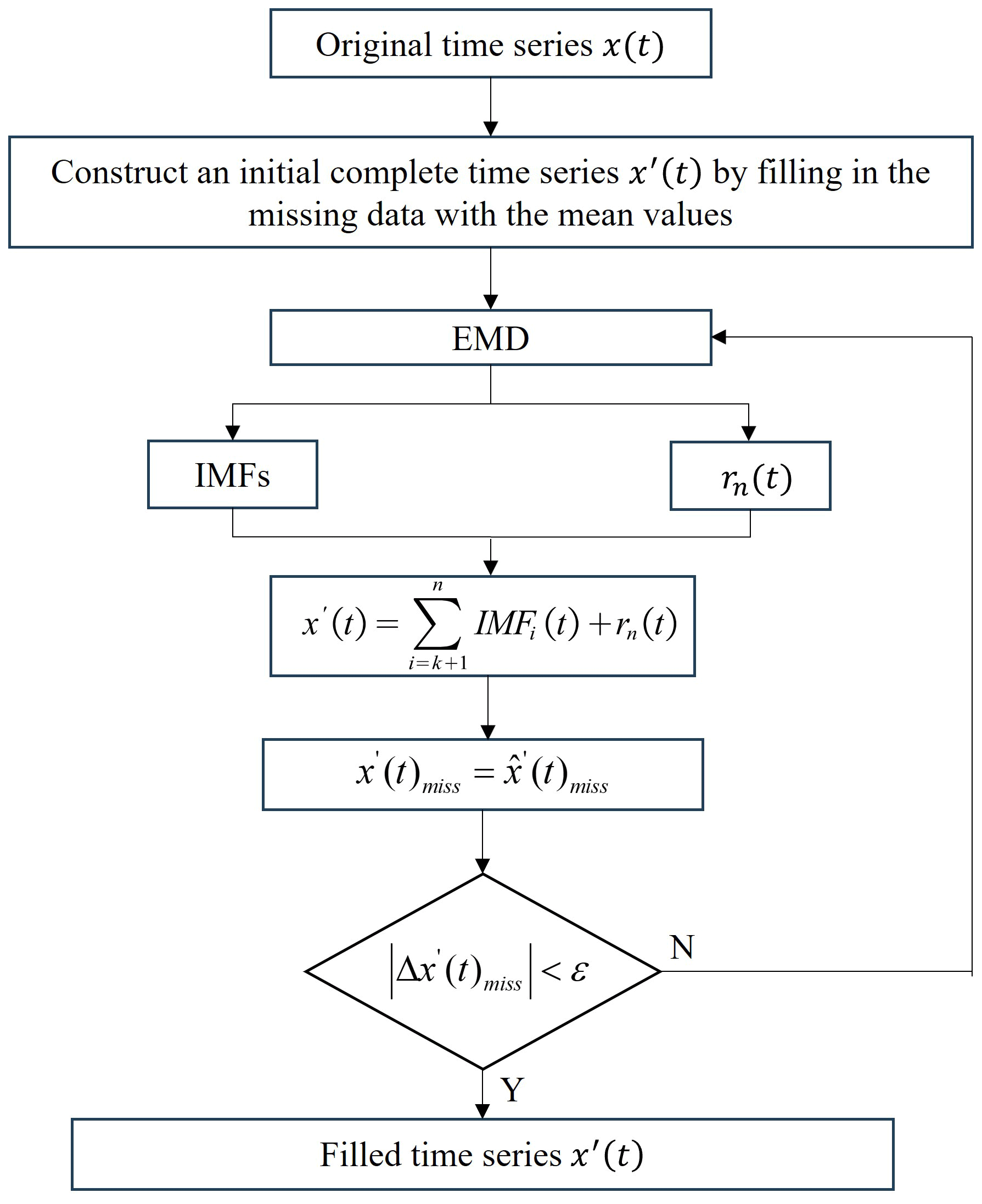
While preprocessing is also essential for adaptive EEMD application, which involves the selection of good continuity and sufficient data, outlier removal, offset detection and missing data filling. Here, the robust interquartile range (IQR) method is used for outlier removal (He et al., 2017), and iterative empirical mode decomposition (IEMD) is utilized for missing data filling (Qiu et al., 2022). The specific IEMD algorithm is seen in Fig. 1. All the missing data are firstly filled with the mean of the observed data to construct an initial complete time series x′(t). Subsequently, traditional EMD decomposes x′(t) into a series of IMF components with frequency from high to low and one residual term. Generally, the boundary IMF index k is determined by the correlation coefficient between the IMF component and the time series x′(t) (Wang et al., 2023), at which it reaches the minimum value for the first time. Then the signals are reconstructed by summing the IMF components after the boundary IMF component and the residual term. The missing data are updated by the corresponding part of the reconstructed signals . When the difference in the missing data |Δx′(t)miss| between two iterations is smaller than ε, the iterative process is terminated, resulting in the final complete time series. Otherwise, the iteration continues. ε represents a threshold (0.005 in this paper) to terminate the iteration process.
With the complete data, the periodic signals can be extracted using the adaptive EEMD method. Firstly, the time series are decomposed into multiple IMFs and corresponding residuals. Secondly, the high-frequency and low-frequency IMFs are determined by the energy value method (Cheng et al., 2006). Thirdly, Lomb spectral analysis is applied to the low-frequency IMFs to identify the periodic signals (Ray et al., 2008). Finally, the IMFs containing periodic signals are selected and combined. Meanwhile, classic LS is employed for comparison. Generally, the function model includes annual, semi-annual, the first to sixth draconitic-year periodic signals (Ray et al., 2008), offsets and after-slips. The after-slip term is typically expressed in the form of logarithmic or exponential functions (Hetland and Hager, 2006; Nishimura, 2014; Tobita, 2016), and in this paper, we adopt an exponential decay function model. Specifically, the functional model can be expressed as
t is the observation time, a is the initial position constant, b is the linear trend, ci and di are the coefficients of the periodic signal (c1 and d1 represent the annual periodic coefficients, while c2 and d2 represent the semi-annual periodic coefficients and others are draconitic-year periodic coefficients), fi is the frequency, ei is the offset magnitude, tj is the moment of offset occurrence, H is the Heaviside function, gz is the after-slip magnitude, tz is the seismic event occurrence time, τz is the relaxation time and n(t) is the noise term.
Last but not least, the assessment of the signal reliability is crucial, which can be measured from different perspectives. Generally, it is measured by correlation coefficients (CCs), root mean square error (RMSE), mean absolute error (MAE), power spectral density index (κ) and signal-to-noise (SNR) (Bos et al., 2008; Chen et al., 2020; Ran et al., 2022). Their specific calculation formulas are as follows:
Xi and Yi are the true signal and prediction signal at the ith sampling point, respectively. and are the means of the two signals. N is the length of the signal. P(f) is the power spectral density of the signal, f is the frequency, P0 and f0 are constants representing the amplitude and reference frequency and κ is the power spectral density index obtained through linear fitting. However, in the practical analysis of stations, there is no true signal present. Therefore, Xi and Yi represent the values at the ith sampling point for the post-processed vertical components (outliers removed, missing data filled and offset corrected) and the extracted periodic signal, respectively. P(f) denotes the power spectral density of the residual signal (Xi−Yi). Due to the true signal known in the simulated experiments, the extracted signal was evaluated using the RMSE and MAE. For the real data analysis, the CC, RMSE, κ and SNR were employed. Specifically, the higher the CC of the extracted periodic signal and the original time series, the more accurate the extraction. A smaller RMSE indicates a more accurate extraction of the periodic signal. The κ of the residuals is used to evaluate the noise characteristics and indirectly reflects the accuracy of the extracted signal, of which the lower absolute values imply more accurate extraction. Similarly, the larger the SNR, the better the periodic model established.
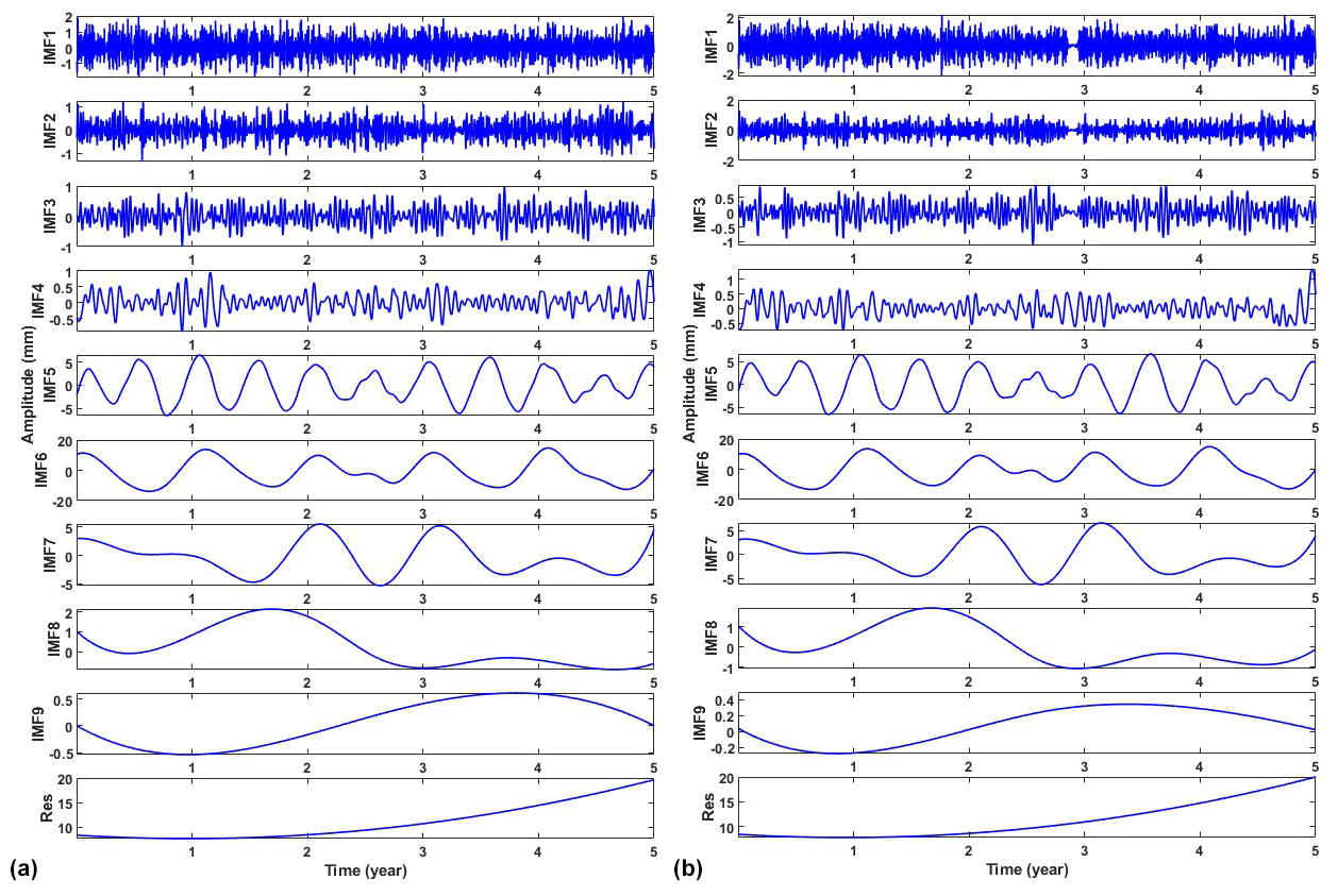
Figure 3Decomposition of filled series with adaptive EEMD: (a) random missing 15 % and (b) consecutive missing 30 d.
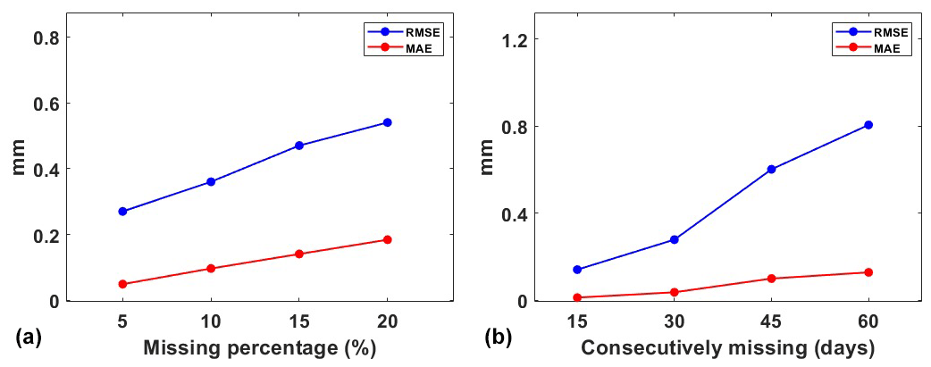
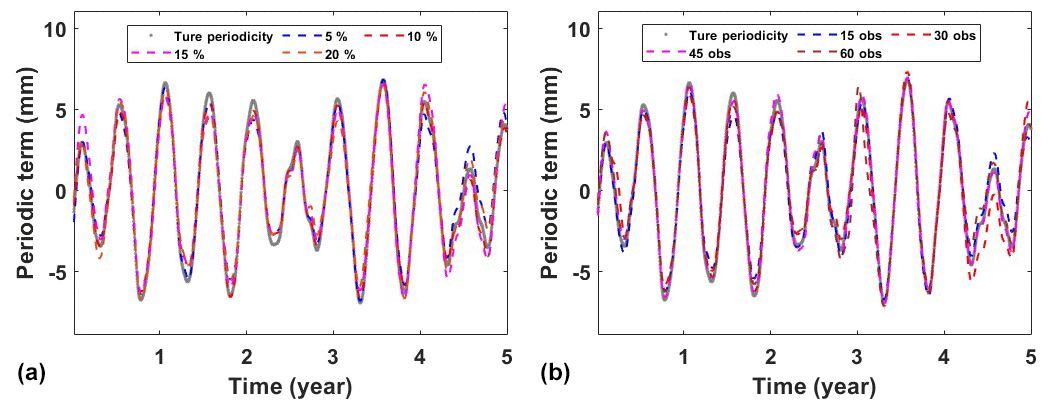
Figure 4The obtained periodic signal and the real periodic signal of (a) randomly missing and (b) consecutively missing.
To test and validate the performance of the adaptive EEMD method, simulation experiments are carried out. In a simplified scenario, only annual and semi-annual periods are simulated as follows.
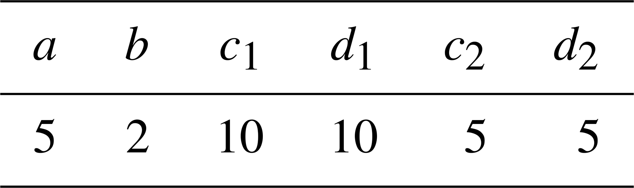
Specifically, the 5-year data x(t) are simulated and are generated with the parameters in Table 1. To be more realistic, not only white noise but also power-law noises are included (Eq. 11). The magnitudes of white noise p(t) and power-law noise q(t) are 0.6 mm and 2 mm−0.6. This means that the power-law spectral index here is −0.60.
Since the missing data and offset are the general cases, these are mainly investigated in this section.
Table 1The simulated parameters in synthetic time series (mm).
3.1 Impact of missing data on adaptive EEMD
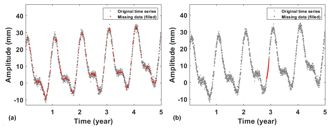
GNSS provides critical daily position time series for geodetic and geophysical studies. However, due to unforeseeable factors such as receiver malfunctions, human errors or deteriorating environmental conditions, the occurrence of missing data is inevitable (Bao et al., 2021). The IEMD method described in Sect. 2 is used in data filling due to its advantages of being efficient and accurate. However, its performance could be influenced by the percentage of missing data. Since there are no true data in the missing epochs, it is impossible to evaluate the performance. Therefore, the missing data in the simulations are artificial deletion from the original data. In practice, data missing may occur randomly or consecutively (Shen et al., 2014). To be more realistic, randomly missing and consecutively missing cases are simulated by deleting data from the original data. For randomly missing, we removed 5 %, 10 %, 15 % and 20 % from the original time series data, while for the simulations of consecutive missing we randomly deleted data for 15, 30, 45 and 60 consecutive days. Here, we present an example with a missing rate of 15 % and a consecutive 30 d missing (Fig. 2). We can see that data marked in red are filled by IEMD, which preserves the same variation of the original time series. The decomposition of the filled data using adaptive EEMD is shown in Fig. 3. From the IMFs, it is easy to identify the simulated annual (IMF6) and semi-annual (IMF5) signals. Figure 4 demonstrates the obtained periodic signal with the real periodic signal. As expected, the results indicate that, with the increase in the percentage of missing data, the extracted periodic signal gradually deviates from the true values. In order to obtain more reliable statistical results, each simulation is carried out 300 times. The mean RMSEs and MAEs of each simulation are presented in Fig. 5. As depicted in the figure, it can be observed that, with the increase in the missing data, both RMSE and MAE gradually increase, which indicates that the stability of the filling results is decreasing and may lead to larger errors. Especially when the random missing data rate reaches 15 %, RMSE and MAE show rapid increases at 0.11 and 0.05, respectively, when consecutively missing data points are between 30 and 45 and the increase in RMSE and MAE is more pronounced, at 0.32 and 0.06, respectively. Therefore, to ensure the accuracy and reliability of adaptive EEMD, the overall random missing rate should be less than 15 %, and the consecutive missing epochs should be less than 30 d.
3.2 Impact of offset on adaptive EEMD
The offsets caused by satellite orbit changes, receiver hardware or software problems, data processing algorithm improvements, and other unknown factors are common in GNSS time series (Gazeaux et al., 2013). For the known offsets, in data preprocessing, the magnitudes of offsets are estimated according to the epochs of earthquake or instrument replacement, and then the known offsets are corrected. However, for the unknown factors, it is difficult to detect the offset time due to the outliers and noises included. While the percentage due to unknown factors can be up to 20 %, its influence cannot be ignored (Griffiths and Ray, 2016). Therefore, it is urgent to identify and correct the offset. Although there are many methods to detect the offset (Wang and Herring, 2019; Tehranchi et al., 2020), neither is 100 % effective. To verify whether the offset correction is essential or not, tests (with and without offset correction) are carried out. Traditionally, manual visual inspection is combined with the STARS method for offset detection, and the LS method is used for offset correction (Rodionov, 2004; Cai, 2020). Since the number and magnitude are the two factors of offsets, these are variables in the simulations. Specifically, the offset number ranges from 2 to 8, with an interval of 2. The simulated offset magnitudes are 0.5σ, 1.0σ, 1.5σ, 2.0σ and 2.5σ mm (Su et al., 2023), with a standard deviation (σ) of the simulated time series (σ=12.70 mm). Also, the simulations are repeated 300 times. Since our focus is the extraction of periodic signals, the effect of simulated offsets on the periodic signals is analyzed. Accordingly, the RMSE and MAE between the periodic signals obtained using the adaptive EEMD method with and without offset correction and the real periodic signal are shown in Fig. 6.
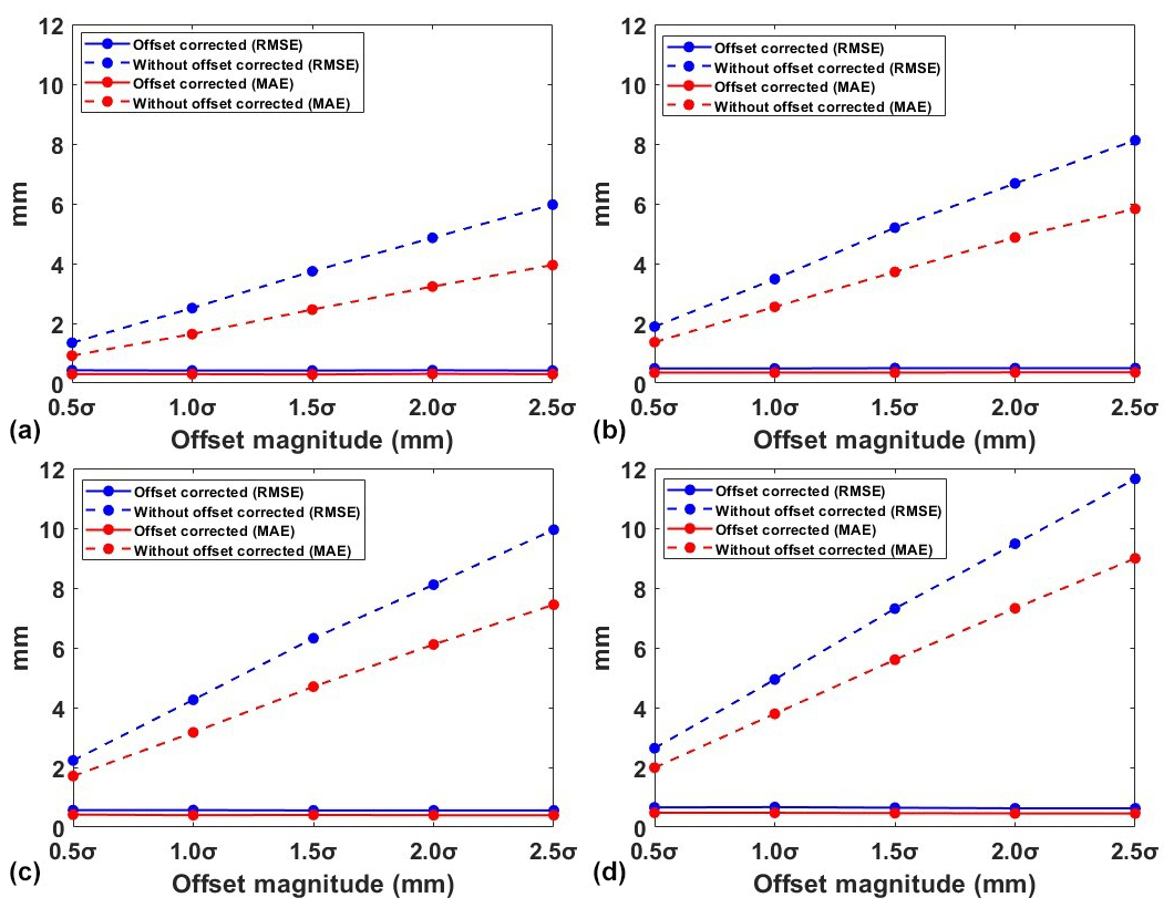
Figure 6Periodic signal RMSE and MAE with and without offset correction of different number and magnitude offsets: (a) two offsets, (b) four offsets, (c) six offsets and (d) eight offsets.
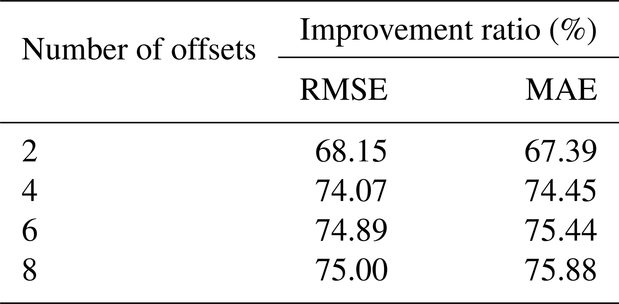
It is found that, with no correction beforehand, RMSE and MAE rapidly increase as the magnitude and the number of offsets increase. With the offset corrected, both RMSE and MAE reveal a substantial decrease. This indicates that, in adaptive EEMD application, the presence of offsets significantly leads to the reduction in the accuracy of periodic signal extraction. Further, the improvement ratio of the offset correction to without correction is shown in Table 2. We can see that, even when the offset magnitude is 0.5σ and the offset number is 2, the ratios for RMSE and MAE are 68.15 % and 67.39 %, respectively. Meanwhile, as the offset number increases, the improvement ratios for RMSE and MAE gradually rise. This indicates the necessity for offset correction even under conditions of small magnitudes. However, these findings are based on all the offsets detected as accurate, although, in reality, this is hard to realize. Thus, we recommend performing offset correction for the adaptive EEMD application in the GNSS coordinate time series analysis.
Table 2The improvement ratios of RMSE and MAE with an offset magnitude of 0.5σ.
4.1 Data sources
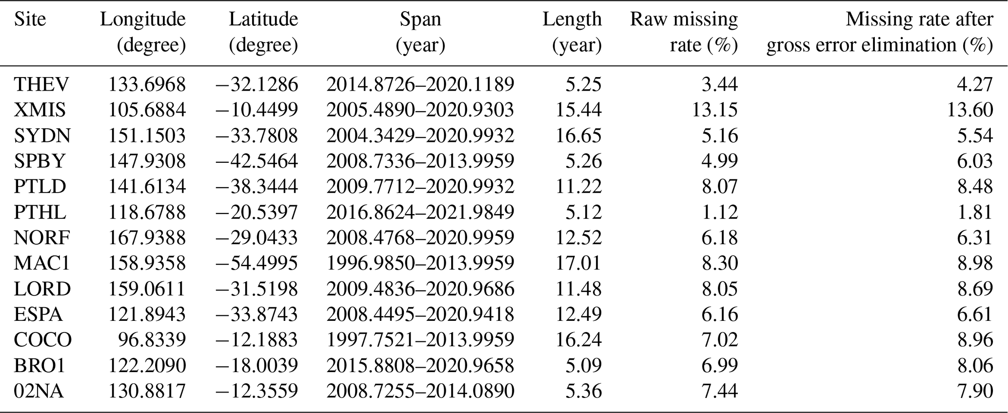
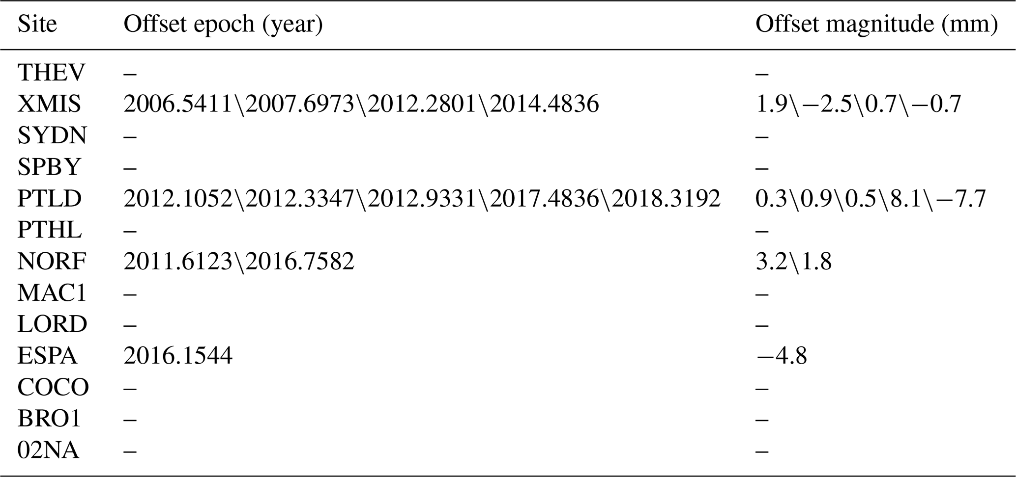
Thirteen GNSS stations located in the Australian region are selected for the study, and their locations are shown in Fig. 7. The vertical components for these selected stations can be downloaded from the SONEL website (https://www.sonel.org/spip.php?page=cgps&lang=en, last access: May 2023). Table 3 provides essential station information, including longitude and latitude coordinates, the time span, the raw missing rate (%) and the missing rate after gross error elimination (%), among which the longest time span is the MAC1 station and the shortest one is the BRO1 station. Additionally, the XMIS station exhibits the highest missing rate after outlier removal, which reaches 13.60 %. The known offset epochs and magnitudes available from the SONEL website, together with the offset that occurred on 12 August 2011 at the NORF station detected with the STARS method along with its magnitude estimated by LS, are shown in Table 4.
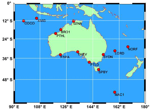
Figure 7Location of the 13 selected GNSS stations in Australia.
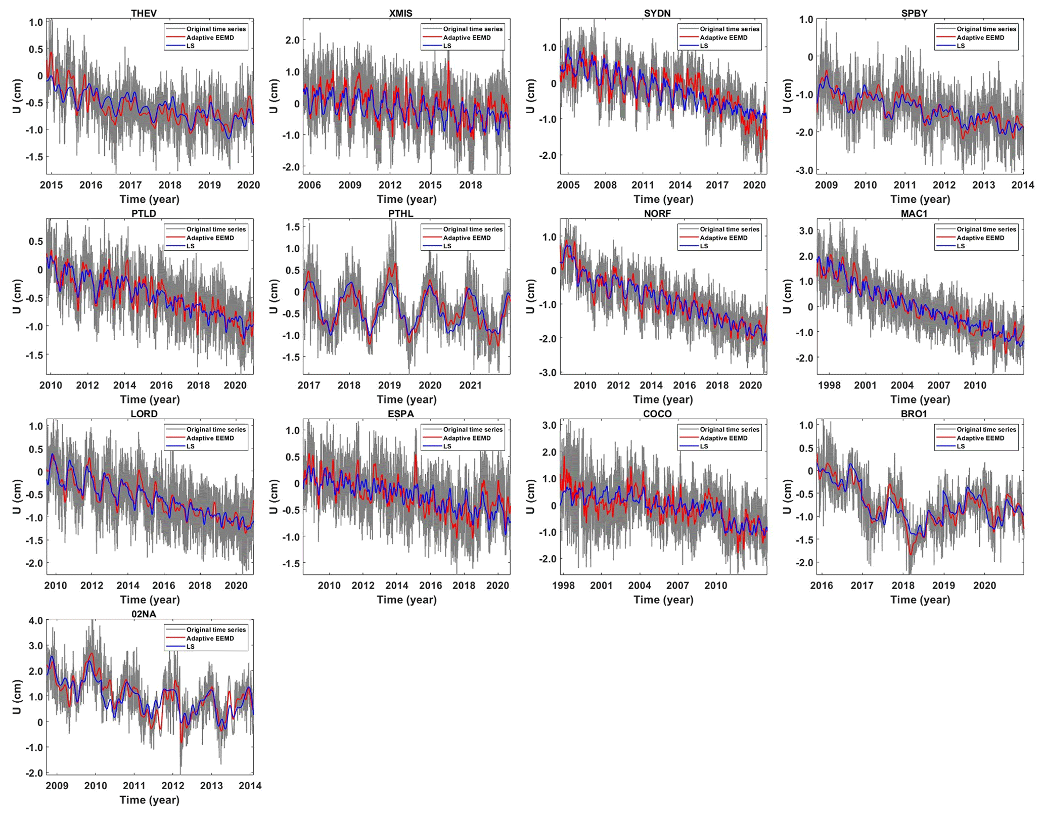
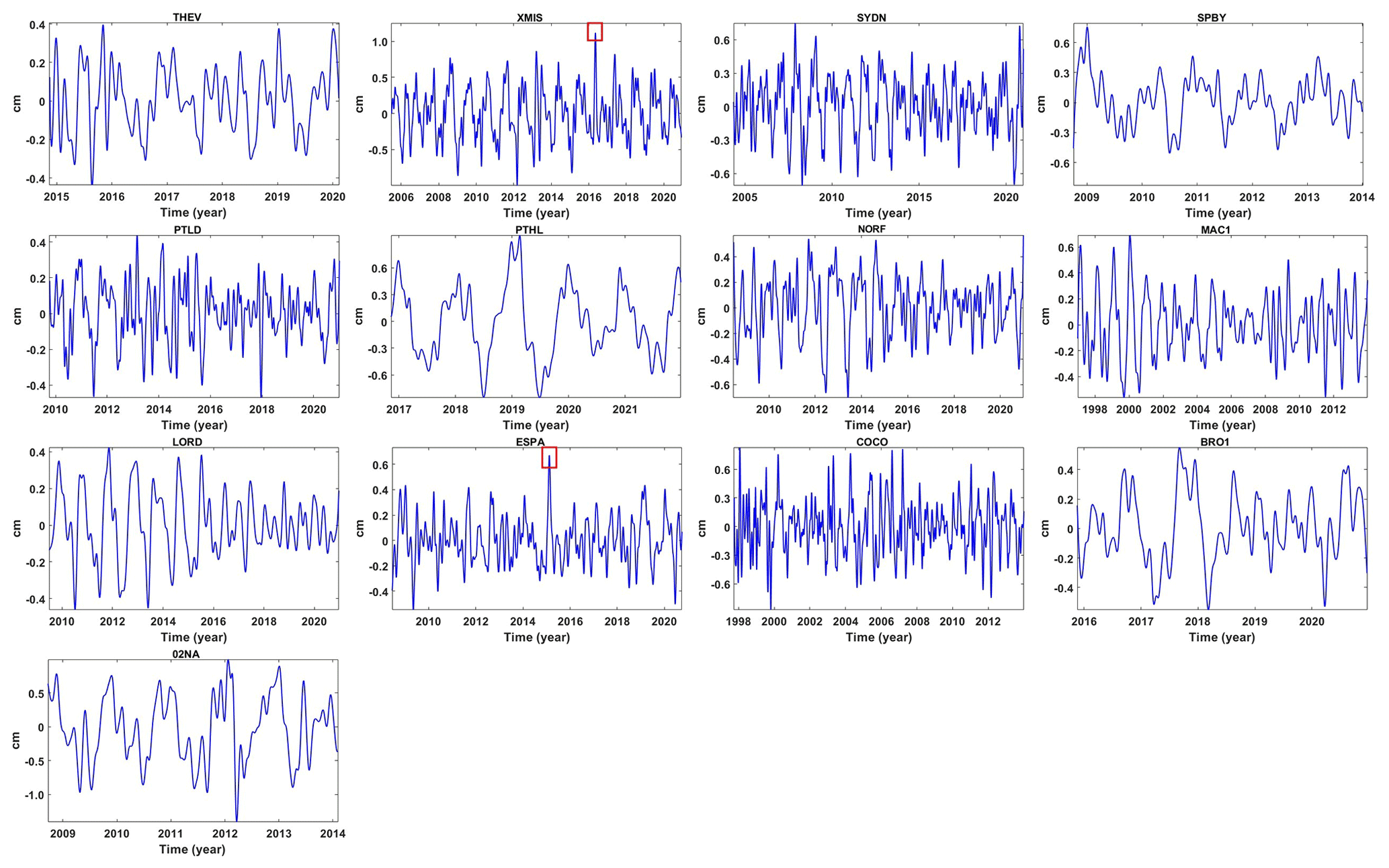
Figure 8Signals derived by the adaptive EEMD and LS of the vertical components at 13 stations.
4.2 Data processing and analysis
In this section, we carry out a comparative analysis of the periodic signal in the vertical component of the 13 selected GNSS stations derived by the adaptive EEMD method and the LS method. Figure 8 presents the post-processed vertical components (outliers removed, missing data filled and the offset corrected) and the extracted signal. It is apparent that the signal extracted is significantly different, from which the adaptive EEMD method shows its advantage in time-varying signal extraction. For example, the signals of XMIS and ESPA demonstrate an apparent peak signal in 2016 and 2015. To further evaluate its performance, comprehensive assessment indicators are displayed in Fig. 9. It is observed that, the higher the CC (Fig. 9a), the lower the RMSE (Fig. 9b), the lower the absolute of κ (Fig. 9c) and the higher the SNR (Fig. 9d) of the adaptive EEMD, which shows its outstanding advantage over LS.
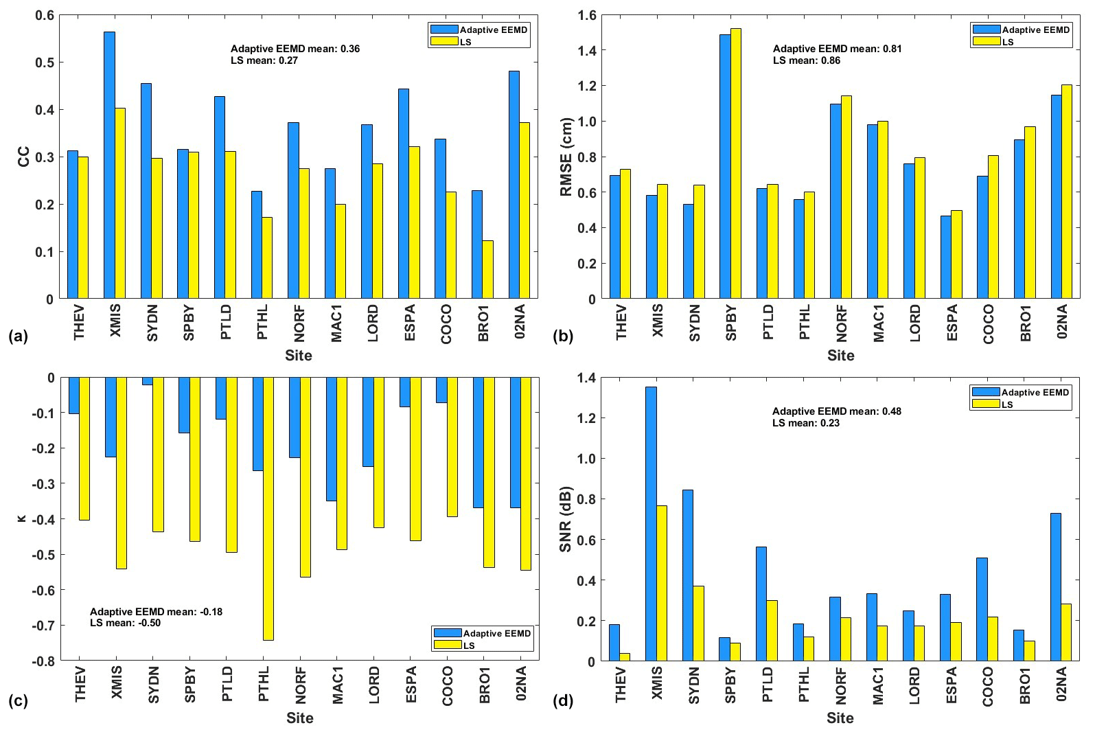
Figure 9Reliability indicators for periodic model assessment: (a) CC, (b) RMSE, (c) κ and (d) SNR.
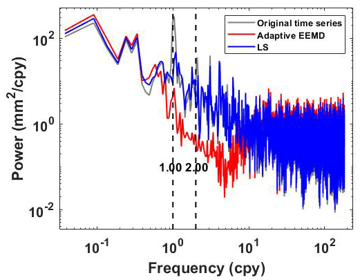
In addition, power spectral stacking analysis is performed on residuals obtained from 13 stations. From Fig. 10 we can see that residuals derived by adaptive EEMD have the lower power of the frequency band in periodic signals than LS. However, it is also noted that the residual signal using the adaptive EEMD method still shows an annual peak. To confirm the significance of this signal within the residual signals, a power spectral significance test is conducted (Horne and Baliunas, 1986; Press et al., 2010), as shown in Fig. 11. The false alarm probability, which is used to estimate the significance of peaks in the power spectrum, indicates the probability of being a result of true signals as opposed to a random noise distribution. Generally, lower values (< 0.01) indicate higher probability. The results indicate that the 1.00 cpy signal is not significant in the residuals. In contrast, the residual signal using the LS method still shows a significant presence of the 1.00 cpy signal. This further highlights the superiority of the adaptive EEMD method in extracting periodic signals.
Moreover, the length of the time series in EEMD application is an important factor to consider, which is essential for investigating the impact on periodic signal extraction. Thus, the aforementioned 13 stations are categorized into two groups based on data length: stations with time series exceeding 10 years (mean time series length of 14.13 years) and stations with time series shorter than 10 years (mean time series length of 5.21 years). Also, significance tests are conducted on stacked residual signals for these two groups of stations. As illustrated in Figs. 12–13, the results demonstrate that, the longer the time series, the better the performance of both methods in extracting periodic signals. Furthermore, the adaptive EEMD method outperforms in both scenarios, which is no matter for data longer or shorter than 10 years.
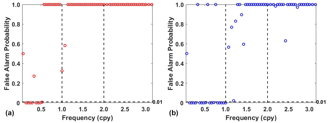
Figure 11Significance test of the residual signal derived from (a) adaptive EEMD and (b) LS.
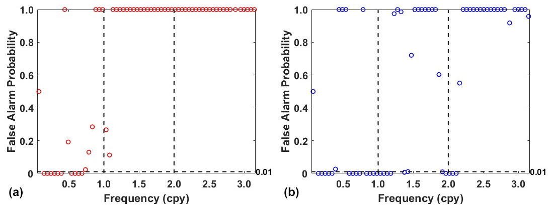
Figure 12Significance test of the residual signal derived from (a) adaptive EEMD and (b) LS for stations with data lower than 10 years.
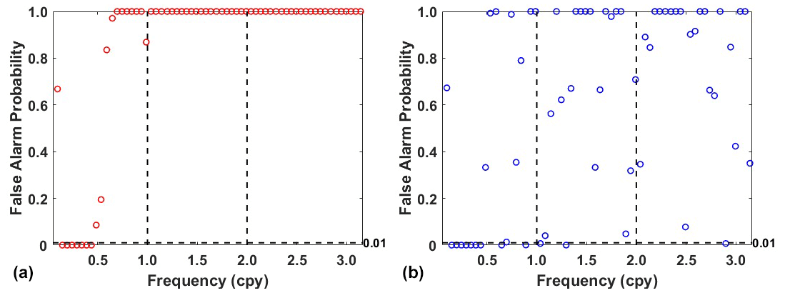
Figure 13Significance test of the residual signal derived from (a) adaptive EEMD and (b) LS for stations with data more than 10 years.
4.3 Discussion
Figure 14 displays all the periodic signals of the 13 stations in the vertical direction. It is evident that all the stations exhibit significant periodic patterns but with varying amplitudes. This may be significantly influenced by geophysical phenomena (Abraha et al., 2017). It is noteworthy that an anomalous peak is observed in the periodic signal of the XMIS station on 2 May 2016 (approximately 2016.35 years) characterized by an approximately twice-larger amplitude than its mean amplitude (which is approximately 0.5 cm). Similar phenomena are also observed at the ESPA station on 10 February 2015 (approximately 2015.11 years). To find a rational explanation, detailed analysis is conducted and utilized hydrological loading data from the EOST Loading Service (http://loading.u-strasbg.fr/listdata.php?dirn=_dicf, last access: July 2023), which possesses a spatial resolution of and a time resolution of 3 h. Additionally, the daily rainfall time series provided by the Australian Bureau of Meteorology (http://www.bom.gov.au/climate/, last access: July 2023) is adopted. Rainfall anomalies are defined as the difference between the daily rainfall and its mean value. The accumulated rainfall anomalies are obtained by summing the daily anomalies with the preceding days' anomalies (Singh et al., 2021). All the possible factors of the two example stations are demonstrated in Fig. 15.
We can see that the extremely low rainfall in the second half of 2015 led to the minimum accumulated rainfall anomaly at the XMIS station on 7 May 2016. The increasing hydrological loading responded to the low rainfall but with a time lag reaching its maximum. According to the reports from the Australian Bureau of Meteorology, the presence of a strong El Niño phenomenon in 2016 (Kennedy et al., 2017) caused the spread of moist water vapor across the Australian continent. The hydrological loading decreased, which was affected by the rainfall directly. Meanwhile, the hydrological loading shows the visible annual features. The CC of 0.50 between hydrological loading data (detrended) and periodic signals for the year 2016 indicates that hydrological loading is one of the primary factors contributing to periodic changes. In addition, the ESPA station also exhibits a similar phenomenon around February 2015, with extremely low rainfall during the first 3 months of the year. This leads to a gradual decrease in accumulated rainfall anomalies, reaching its minimum on 29 March 2015. Hydrological loading during the same period reaches its current peak. The CC between the hydrological loading data (detrended) and the 2015 periodic signal is 0.57. This further emphasizes the significance of hydrological loading variations in relation to periodic changes. In summary, the primary characteristics of periodic variations are induced by hydrological loading, and other factors may also affect the periodic signals to some extent, which provides a direction for future research to explore in depth.
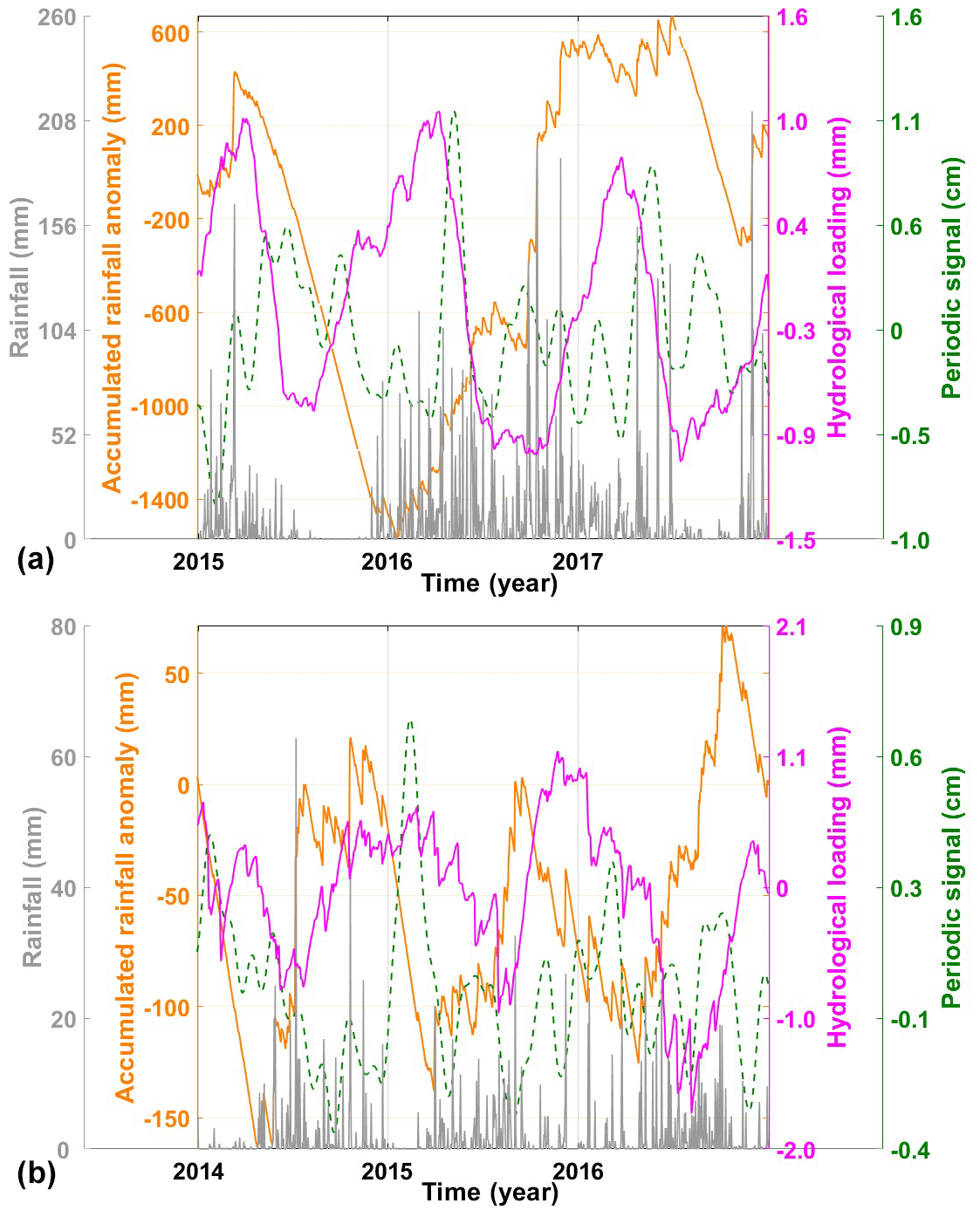
Figure 15Abnormal periodic signal analysis at (a) the XMIS station (2015–2017) and (b) the ESPA station (2014–2016).
This paper employed the adaptive EEMD method for more efficient and accurate extraction of periodic signals. The simulations are conducted focusing on the inevitable missing data and offset issues. The results revealed that, with the missing data filled with the IEMD method, the adaptive EEMD method exhibits efficiency in signal extraction. As expected, when the percentage of missing data increases, the extracted periodic signals may gradually deviate from the true values. Specifically, for the missing random data, when the missing rate reaches 15 %, RMSE and MAE show rapid increases at 0.11 and 0.05, respectively. For the missing consecutive data, when missing lasts for 1 month, the increases in RMSE and MAE also reach their maximum values at 0.32 and 0.06, respectively. Therefore, it is recommended that high accuracy could reach the overall random missing rate below 15 % and avoid consecutive missing epochs exceeding 30 d when dealing with GNSS coordinate time series. Regarding the offset, it is apparent that correction beforehand is essential since RMSE and MAE are markedly reduced. This also means that the offset detection and correction cannot be ignored for the adaptive EEMD application. For the processing vertical component from 13 GNSS stations in Australia, adaptive EEMD shows its advantage over LS. The mean values for CC, RMSE, κ and SNR for the adaptive EEMD are 0.36, 0.81, −0.18 and 0.48, respectively, while the mean values for LS are 0.27, 0.86, −0.50 and 0.23. Moreover, significance tests are conducted on the residuals, which further confirms that annual signals still exist in the residuals for LS but not for the EEMD. The periodic signals of the 13 investigated GNSS stations reflect the time-varying characteristics. It is found that there are significant variations of the XMIS in 2016 and ESPA in 2015. Their CC with hydrological loading are 0.50 and 0.57, respectively, indicating that hydrological loading is one primary factor contributing to the periodic variations.
In conclusion, this research highlights the advantages of the adaptive EEMD method for periodic signal extraction no matter the synthetic or real GNSS coordinate time series analysis. The handling of the missing data and offset is firstly comprehensively investigated, which provides a helpful solution to preprocessing EEMD. Furthermore, it reveals the time-varying characteristics of the periodic signal, which is favorable in the subsequent trend analysis of the GNSS stations in the SONEL network. Without doubt, the adaptive EEMD can also be applied not only to the GNSS coordinate time series, but also other geophysical data.
The Australian region GNSS station data used in this study are all available from the SONEL website (https://www.sonel.org/spip.php?page=cgps&lang=en, SONEL, 2023). The hydrological loading data are available from the EOST Loading Service (http://loading.u-strasbg.fr/listdata.php?dirn=dicf, EOST Loading Service, 2023). Additionally, the daily rainfall time series can be obtained from the official website of the Australian Bureau of Meteorology (http://www.bom.gov.au/climate/data/index.shtml?bookmark=136, Australian Burcau of Meteorology, 2023).
WL: conceptualization, methodology, investigation, formal analysis, writing – original draft, funding acquisition. JG: data curation, formal analysis, writing – original draft.
The contact author has declared that neither of the authors has any competing interests.
Publisher's note: Copernicus Publications remains neutral with regard to jurisdictional claims made in the text, published maps, institutional affiliations, or any other geographical representation in this paper. While Copernicus Publications makes every effort to include appropriate place names, the final responsibility lies with the authors.
This research was funded by the National Natural Science Foundation of China (grant no. 41904011), Laoshan Laboratory (grant nos. LSKJ202205104 and LSKJ202205104_03) and the Shandong Provincial Natural Science Foundation (grant no. ZR2019QD003).
This research has been supported by the Laoshan Laboratory (grant nos. LSKJ202205104 and LSKJ202205104_03).
This paper was edited by Norbert Marwan and reviewed by two anonymous referees.
Agnieszka, W. and Dawid, K.: Modeling seasonal oscillations in GNSS time series with Complementary Ensemble Empirical Mode Decomposition, GPS Solut., 26, 101, https://doi.org/10.1007/s10291-022-01288-2, 2022.
Abraha, K. E., Teferle, F. N., Hunegnaw, A., and Dach, R.: GNSS related periodic signals in coordinate time-series from Precise Point Positioning, Geophys. J. Int., 208, 1449–1464, https://doi.org/10.1093/gji/ggw467, 2017.
Australian Burcau of Meteorology: http://www.bom.gov.au/climate/data/index.shtml?bookmark=136, last access: July 2023.
Bao, Z., Chang, G., Zhang, L., Chen, G., and Zhang, S.: Filling missing values of multi-station GNSS coordinate time series based on matrix completion, Measurement, 183, 109862, https://doi.org/10.1016/J.MEASUREMENT.2021.109862, 2021.
Bennett, R. A.: Instantaneous deformation from continuous GPS: Contributions from quasi-periodic loads, Geophys. J. Int., 174, 1052–1064, https://doi.org/10.1111/j.1365-246X.2008.03846.x, 2008.
Blewitt, G., Kreemer, C., Hammond, W. C., Plag, H. P., Stein, S., and Okal, E.: Rapid determination of earthquake magnitude using GPS for tsunami warning systems, Geophys. Res. Lett., 33, L11309, https://doi.org/10.1029/2006GL026145, 2006.
Bos, M. S., Fernandes, R. M. S., Williams, S. D. P., and Bastos, L.: Fast error analysis of continuous GPS observations, J. Geodesy, 82, 157–166, https://doi.org/10.1007/s00190-007-0165-x, 2008.
Bos, M. S., Bastos, L., and Fernandes, R. M. S.: The influence of seasonal signals on the estimation of the tectonic motion in short continuous GPS time-series, J. Geodyn., 49, 205–209, https://doi.org/10.1016/j.jog.2009.10.005, 2010.
Cai, F.: Study on global distribution laws and partial mechanisms of nonlinear variations of GNSS stations' coordinates, M.S. thesis, Strategic Support Force Information Engineering University, https://doi.org/10.27188/d.cnki.gzjxu.2020.000068, 2020 (in Chinese).
Calais, E., Gonzalez, O. F., Arango-Arias, E. D., Moreno, B., Palau, R., Cutie, M., Diez, E., Montenegro, C., Rodriguez Roche, E., Garcia, J., Castellanos, E., and Symithe, S.: Current deformation along the northern Caribbean plate boundary from GNSS measurements in Cuba, Tectonophysics, 868, 230068, https://doi.org/10.1016/j.tecto.2023.230068, 2023.
Chen, B., Bian, J., Ding, K., Wu, H., and Li, H.: Extracting seasonal signals in GNSS coordinate time series via weighted nuclear norm minimization, Remote. Sens.-Basel, 12, 2027, https://doi.org/10.3390/rs12122027, 2020.
Cheng, J., Yu, D., and Yu, Y.: Research on the intrinsic mode function (IMF) criterion in EMD method, Mech. Syst. Signal. Pr., 20, 817–824, https://doi.org/10.1016/j.ymssp.2005.09.011, 2006.
Costantino, G., Giffard-Roisin, S., Radiguet, M., Dalla Mura, M., Marsan, D., and Socquet, A.: Multi-station deep learning on geodetic time series detects slow slip events in Cascadia, Commun. Earth Environ., 4, 435, https://doi.org/10.1038/s43247-023-01107-7, 2023.
Davis, J. L., Wernicke, B. P., and Tamisiea, M. E.: On seasonal signals in geodetic time series, J. Geophys. Res., 117, B01403, https://doi.org/10.1029/2011JB008690, 2012.
Din, A. H. M., Zulkifli, N. A., Hamden, M. H., and Wan Aris, W. A.: Sea level trend over Malaysian seas from multi-mission satellite altimetry and vertical land motion corrected tidal data, Adv. Space. Res., 63, 3452–3472, https://doi.org/10.1016/j.asr.2019.02.022, 2019.
Dong, D., Fang, P., Bock, Y., Cheng, M. K., and Miyazaki, S.: Anatomy of apparent seasonal variations from GPS-derived site position time series, J. Geophys. Res., 107, ETG 9-1–ETG 9-16, https://doi.org/10.1029/2001JB000573, 2002.
EOST Loading Service: http://loading.u-strasbg.fr/listdata.php?dirn=dicf, last access: May 2023.
Gazeaux, J., Williams, S., King, M., Bos, M., Dach, R., Deo, M., Moore, A. W., Ostini, L., Petrie, E., Roggero, M., Teferle, F. N., Olivares, G., and Webb, F. H.: Detecting offsets in GPS time series: First results from the detection of offsets in GPS experiment, J. Geoghys. Res.-Sol. Ea., 118, 2397–2407, https://doi.org/10.1002/jgrb.50152, 2013.
Griffiths, J. and Ray, J.: Impacts of GNSS position offsets on global frame stability, Geophys. J. Int., 204, 480–487, https://doi.org/10.1093/gji/ggv455, 2016.
Gülal, E., Erdoğan, H., and Tiryakioğlu, İ.: Research on the stability analysis of GNSS reference stations network by time series analysis, Digit. Signal. Process., 23, 1945–1957, https://doi.org/10.1016/j.dsp.2013.06.014, 2013.
He, X., Montillet, J. P., Fernandes, R., Bos, M., Yu, K., Hua, X. and Jiang, W.: Review of current GPS methodologies for producing accurate time series and their error sources, J. Geodyn., 106, 12–29, https://doi.org/10.1016/j.jog.2017.01.004, 2017.
Hetland, E. A. and Hager, B. H.: The effects of rheological layering on post-seismic deformation, Geophys. J. Int., 166, 277–292, https://doi.org/10.1111/j.1365-246X.2006.02974.x, 2006.
Horne, J. H. and Baliunas, S. L.: A prescription for period analysis of unevenly sampled time series, Astrophys. J., 302, 757–763, 1986.
Huang, N. E., Shen, Z., Long, S. R., Wu, M. C., Shih, H. H., Zheng, Q., Yen, N-C. Tung, C. C. and Liu, H. H.: The empirical mode decomposition and the Hilbert spectrum for nonlinear and non-stationary time series analysis, P. Roy. Soc. Lond. Ser. A-Math., 454, 903–995, https://doi.org/10.1098/rspa.1998.0193, 1998.
Huang, N. E., Shen, Z., and Long, S. R.: A new view of nonlinear water waves: the Hilbert spectrum, Annu. Rev. Fluid. Mech., 31, 417–457, https://doi.org/10.1146/annurev.fluid.31.1.417, 1999.
Huang, Y., Schmitt, F. G., Lu, Z., and Liu, Y.: Analysis of daily river flow fluctuations using empirical mode decomposition and arbitrary order Hilbert spectral analysis, J. Hydrol., 373, 103–111, https://doi.org/10.1016/j.jhydrol.2009.04.015, 2009.
Ide, S. and Tanaka, Y.: Controls on plate motion by oscillating tidal stress: Evidence from deep tremors in western Japan, Geophys. Res. Lett., 41, 3842–3850, https://doi.org/10.1002/2014GL060035, 2014.
Johnson, C. W., Lau, N., and Borsa, A.: An assessment of global positioning system velocity uncertainty in California, Earth Space Sci., 8, e2020EA001345, https://doi.org/10.1029/2020EA001345, 2021.
Kennedy, J., Dunn, R., McCarthy, M., Titchner, H., and Morice, C.: Global and regional climate in 2016, Weather, 72, 219–225, https://doi.org/10.1002/wea.3042, 2017.
Klos, A., Olivares, G., Teferle, F. N., Hunegnaw, A., and Bogusz, J.: On the combined effect of periodic signals and colored noise on velocity uncertainties, GPS Solut., 22, 1, https://doi.org/10.1007/s10291-017-0674-x, 2018.
Kopsinis, Y. and McLaughlin, S.: Improved EMD using doubly-iterative sifting and high order spline interpolation, Eurasip. J. Adv. Sig. Pr., 2008, 128293, https://doi.org/10.1155/2008/128293, 2008.
Li, W.: Data adaptive analysis on vertical surface deformation derived from daily ITSG-Grace2018 model, Sensors, 20, 4477, https://doi.org/10.3390/s20164477, 2020.
Li, W. and Shen, Y.: Detection and analysis of velocity and amplitude changes in GNSS coordinate sequences, Journal of Tongji University, 42, 604–610, https://doi.org/10.3969/j.issn.0253-374x.2014.04.017, 2014 (in Chinese).
Liu, X., Chen, W., and Mao, A.: An adaptive optimization EEMD method and its application in bearing fault detection, ResearchSquare [preprint], https://doi.org/10.21203/rs.3.rs-2615109/v1, 28 February 2023.
Munekane, H.: Modeling long-term volcanic deformation at Kusatsu-Shirane and Asama volcanoes, Japan, using the GNSS coordinate time series, Earth. Planets Space, 73, 192, https://doi.org/10.1186/s40623-021-01512-2, 2021.
Nishimura, T.: Pre-, co-, and post-seismic deformation of the 2011 Tohoku-oki earthquake and its implication to a paradox in short-term and long-term deformation, J. Disaster Res., 9, 294–302, https://doi.org/10.20965/jdr.2014.p0294, 2014.
Peng, W., Dai, W. J., Santerre, R., Cai, C. S., and Kuang, C. L.: GNSS vertical coordinate time series analysis using single-channel independent component analysis method, Phys. Eng. Sci., 454, 903–995, https://doi.org/10.1007/s00024-016-1309-9, 2018.
Press, W. H., Teukolsky, S. A., Vetterling, W. T., and Flannery, B. P.: Numerical Recipes: The Art of Scientific Computing, 3rd Edn., Cambridge University Press, ISBN 9780521880688, 2010.
Qiu, X., Wang, F., Zhou, Y., and Zhou, S.: Iteration empirical mode decomposition method for filling the missing data of GNSS position time series, Acta. Geodyn. Geomater., 19, 271–279, https://doi.org/10.13168/AGG.2022.0012, 2022.
Rodionov, N. S.: A sequential algorithm for testing climate regime shifts, Geophys. Res. Lett., 31, L09204, https://doi.org/10.1029/2004GL019448, 2004.
Ran, J., Bian, J., Chen, G., Zhang, Y., and Liu, W.: A truncated nuclear norm regularization model for signal extraction from GNSS coordinate time series, Adv. Space Res., 70, 336–349, https://doi.org/10.1016/j.asr.2022.04.040, 2022.
Ray, J., Altamimi, Z., Collilieux, X., and Van Dam, T.: Anomalous harmonics in the spectra of GPS position estimates, GPS Solut., 12, 55–64, https://doi.org/10.1007/s10291-007-0067-7, 2008.
Scaramuzza, S., Dach, R., Beutler, G., Arnold, D., Sušnik, A., and Jäggi, A.: Dependency of geodynamic parameters on the GNSS constellation, J. Geodesy, 92, 93–104, https://doi.org/10.1007/s00190-017-1047-5, 2017.
Shen, Y., Li, W., Xu, G., and Li, B.: Spatiotemporal filtering of regional GNSS network's position time series with missing data using principle component analysis, J. Geodesy, 88, 1–12, https://doi.org/10.1007/s00190-013-0663-y, 2014.
Singh, A., Reager, J. T., and Behrangi, A.: Estimation of hydrological drought recovery based on precipitation and Gravity Recovery and Climate Experiment (GRACE) water storage deficit, Hydrol. Earth Syst. Sci., 25, 511–526, https://doi.org/10.5194/hess-25-511-2021, 2021.
SONEL: https://www.sonel.org/spip.php?page=cgps&lang=en, last access: May 2023.
Sorin, N., NorbertSzabolcs, S., Ahmed, E., Michal, A., Zinovy, M., Ilie, N. E., Jacek, K., and Kamil, M.: Implication between geophysical events and the variation of seasonal signal determined in GNSS position time series, Remote. Sens.-Basel, 13, 3478–3478, https://doi.org/10.3390/RS13173478, 2021.
Su, L., Zhai, H., Wang, Q., and Tian, X.: Detecting offsets in GPS coordinate time series based on SSA method, Journal of Geodesy and Geodynamics, 43, 464–466, https://doi.org/10.14075/j.jgg.2023.05.005, 2023 (in Chinese).
Tehranchi, R., Moghtased-Azar, K., and Safari, A.: A new statistical test based on the WR for detecting offsets in GPS experiment, Earth Space Sci., 7, e2019EA000810, https://doi.org/10.1029/2019EA000810, 2020.
Tobita, M.: Combined logarithmic and exponential function model for fitting postseismic GNSS time series after 2011 Tohoku-Oki earthquake, Earth. Planets Space, 68, 1–12, 2016.
Van Dam, T., Wahr, J., Milly, P. C. D., Shmakin, A. B., Blewitt, G., Lavallée, D., and Larson, K. M.: Crustal displacements due to continental water loading, Geophys. Res. Lett., 28, 651–654, https://doi.org/10.1029/2000GL012120, 2001.
Wang, J., Ding, K., Sun, H., Zhang, G., and Chen, X.: Noise reduction and periodic signal extraction for GNSS height data in the study of vertical deformation, Geodesy and Geodynamics, 14, 573–581, https://doi.org/10.1016/j.geog.2023.07.002, 2023.
Wang, K., Jiang, W., Chen, H., An, X., Zhou, X., Yuan, P., and Chen, Q.: Analysis of seasonal signal in GPS short-baseline time series, Pure. Appl. Geophys., 175, 3485–3509, https://doi.org/10.1007/s00024-018-1871-4, 2018.
Wang, L. and Herring, T.: Impact of estimating position offsets on the uncertainties of GNSS site velocity estimates, J. Geophys. Res.-Sol. Ea., 124, 13452–13467, https://doi.org/10.1029/2019JB017705, 2019.
Willen, M. O., Horwath, M., Groh, A., Helm, V., Uebbing, B., and Kusche, J.: Feasibility of a global inversion for spatially resolved glacial isostatic adjustment and ice sheet mass changes proven in simulation experiments, J. Geodesy, 96, 75, https://doi.org/10.1007/S00190-022-01651-8, 2022.
Wu, F. and Qu, L.: An improved method for restraining the end effect in empirical mode decomposition and its applications to the fault diagnosis of large rotating machinery, J. Sound. Vib., 314, 586–602, https://doi.org/10.1016/j.jsv.2008.01.020, 2008.
Wu, Z. and Huang, N. E.: Ensemble empirical mode decomposition: a noise-assisted data analysis method, Advances in Adaptive Data Analysis, 1, 1–41, https://doi.org/10.1142/S1793536909000047, 2009.
Zaccagnino, D., Vespe, F., and Doglioni, C.: Tidal modulation of plate motions, Earth-Sci. Rev., 205, 103179, https://doi.org/10.1016/j.earscirev.2020.103179, 2020.
Zhou, X., Yang, Y., Chen, Q., Fan, W., and Ma, Y.: A robust trend estimator for GNSS time series in the presence of complex periodicity and its evaluation on multi-source products of IGS and IGMAS, GPS Solut., 26, 103, https://doi.org/10.1007/s10291-022-01271-x, 2022.