the Creative Commons Attribution 4.0 License.
the Creative Commons Attribution 4.0 License.
 | 26 Jun 2024
A quest for precipitation attractors in weather radar archives
Loris Foresti
Bernat Puigdomènech Treserras
Daniele Nerini
Aitor Atencia
Marco Gabella
Ioannis V. Sideris
Urs Germann
Isztar Zawadzki
Archives of composite weather radar images represent an invaluable resource to study the predictability of precipitation. In this paper, we compare two distinct approaches to construct empirical low-dimensional attractors from radar precipitation fields. In the first approach, the phase space variables of the attractor are defined using the domain-scale statistics of precipitation fields, such as the mean precipitation, fraction of rain, and spatial and temporal correlations. The second type of attractor considers the spatial distribution of precipitation and is built by principal component analysis (PCA). For both attractors, we investigate the density of trajectories in phase space, growth of errors from analogue states, and fractal properties. To represent different scales and climatic and orographic conditions, the analyses are done using multi-year radar archives over the continental United States ( km2, 21 years) and the Swiss Alpine region ( km2, 6 years).
- Article
(16140 KB) - Full-text XML
- BibTeX
- EndNote


Precipitation is challenging to forecast. The difficulty is due to its large space–time variability (e.g. Lovejoy and Schertzer, 2013), the many non-linear processes involved (e.g. Houze, 2014), and the resulting chaotic behaviour of the atmosphere (e.g. Lorenz, 1963), among others.
As a result, a rapid loss of precipitation predictability is observed for both extrapolation-based nowcasting and numerical weather prediction (NPW)-based forecasting (e.g. Surcel et al., 2015). Such limits to predictability drive the need for more accurate estimates of forecast uncertainty to enable informed decision-making.
Lorenz (1996) defines two types of predictability:
-
intrinsic predictability: “the extent to which prediction is possible if an optimum procedure is used”;
-
practical predictability: “the extent to which we are able to predict by the best-known procedures”.
The goal of forecasting is to design models whose practical predictability is as close as possible to the intrinsic predictability while representing the remaining uncertainty.
Studies on atmospheric predictability are either model-based or observation-based: see a review in Lorenz (1996) and Germann et al. (2006b). Modelling studies use either idealized systems of equations (e.g. Lorenz, 1963) or NWP models (e.g. Palmer and Hagedorn, 2006). One disadvantage of such methods is related to the strong assumptions about how precipitation processes are represented in the models.
Observation-based predictability studies comprise statistical extrapolation methods (e.g. Germann et al., 2006b) and naturally occurring analogues (e.g. Lorenz, 1969). Common challenges are related to the presence of measurement uncertainty, the assumption of attractor smoothness (e.g. Takens, 1981) and the limited size of archives (e.g. Toth, 1991; Van Den Dool, 1994), which only allows analogues of “mediocre” quality to be found (Lorenz, 1969). Precipitation brings further challenges due to its truncated non-Gaussian distribution and intermittent and multifractal properties (Schertzer and Lovejoy, 1987; Lovejoy and Schertzer, 2013).
Atencia and Zawadzki (2017) used the Lorenz63 system to compare the growth of errors (spread) from analogue states with the one obtained from standard perturbation techniques used in NWP ensemble forecasting. They showed that analogues display a similar initial error growth but contain more information throughout the forecast. Therefore, despite the limitations of observation-based studies, analogues have good potential to complement predictability studies.
Inspired by Atencia et al. (2013), this study aims to construct low-dimensional attractors from weather radar archives to shed new light on the intrinsic predictability of precipitation. We compare two distinct approaches to construct the attractor. The first is a deductive approach based on prior knowledge, where the phase space variables are defined based on domain expertise and (forecast) application requirements. The second is an inductive approach, where the phase space variables are extracted from the data without prior assumptions (except those required by principal component analysis, PCA). This research has an exploratory character and focuses on what worked and did not work in our quest for the precipitation attractor. The careful reader will notice that the methodology of the Swiss and US attractors is not 100 % consistent. Indeed, most of the research started independently and only converged into this paper at a later stage. Less successful experiments in one attractor were not replicated onto the other, where we preferred to explore more promising directions. Consequently, the results of the paper will not be interpreted in quantitative and absolute terms, but rather in qualitative terms. The investigation of the qualitative differences between the two attractors, in both the methodology and the results, triggered fruitful discussions.
In this paper, we want to answer the following questions.
-
What do we learn about the predictability of precipitation from weather radar archives?
-
How do we define the phase space of the attractor?
-
What is the typical growth of errors from analogues?
-
How does predictability depend on scale?
-
In which way is the attractor relevant for short-term precipitation forecasting and stochastic simulation?
The paper is structured as follows. Section 2 describes the two radar archives and the conceptual framework. Section 3 defines the attractor based on domain-scale statistics and presents analyses of its properties. The same is done in Sect. 4 using principal component analysis. Section 5 concludes the paper and discusses future perspectives. Statistical techniques are detailed in the Appendix.
2.1 Archives of composite radar images
The US and Swiss radar datasets are described in Table 1. The US data are produced by the operational S-band Weather Surveillance Radar-1988 Doppler network (WSR-88D) covering the continental United States (CONUS). The archive spans a 21-year period from 1996 to 2016 and was obtained by interpolating four different radar composite products to a common 4 km resolution grid. Radar products comprise the maximum echo from any radar (1996–2007) as well as more advanced products removing ground clutter and blending of multiple radars; see more details in Atencia and Zawadzki (2015) and Fabry et al. (2017). For computational reasons, the temporal resolution was reduced from 5 to 15 min and a smaller domain of 4096×4096 km2 was extracted (see Fig. 1). When needed, data were upscaled by averaging the rain rate in linear units using the Marshall–Palmer Z–R relationship Z=300R1.5. Note that radar visibility on the Rocky Mountains is rather limited by the large inter-radar distances, which is the reason why the domain is cut (see Appendix F).
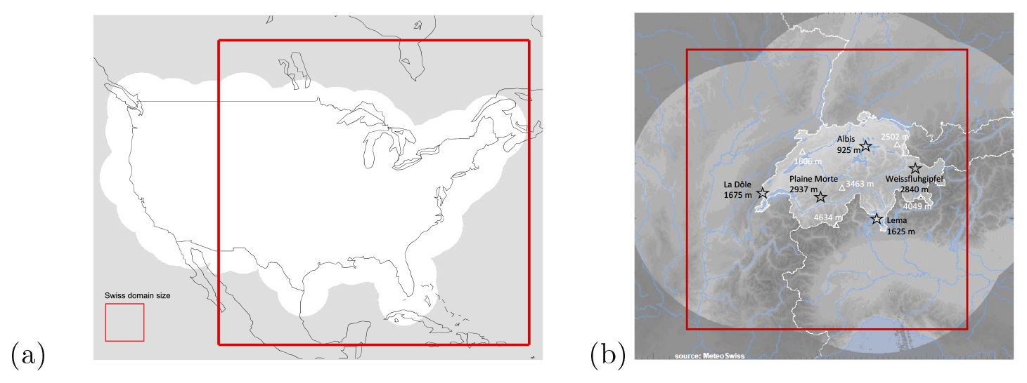
Figure 1(a) Continental US analysis domain of 4096×4096 km2 (white background indicates the radar composite coverage). (b) Swiss analysis domain of 512×512 km2 (the lighter grey background indicates the radar composite coverage, the black text the location and height of weather radars, and the white text the location and height of important mountain peaks). The US domain surface is 64 times larger than the Swiss domain.
Table 1Characteristics of the Swiss and US radar datasets. * Number of images with wet area ratio ≥ 5 %.
The Swiss data comprise the quantitative precipitation estimation (QPE) product, which integrates measurements from three Doppler C-band weather radars (Germann et al., 2006a). The archive covers a 6-year period from 2005 to 2010 and has a spatial resolution of 1 km and a temporal resolution of 5 min. The domain was reduced to a square 512 km grid centred over Switzerland (see Fig. 3a). The radar network was upgraded to dual polarization in 2011 and equipped with two new radars in 2014 and 2016 to improve the coverage in the inner Alpine valleys (e.g. Germann et al., 2022). To avoid temporal inhomogeneity in the archive introduced by the switch to the new radar generation, in this study we did not include data after 2011.
Radar-based QPE is inevitably affected by uncertainty due to e.g. the Z–R relationship, variability of the vertical profile of reflectivity, signal attenuation and residual clutter (e.g. Villarini and Krajewski, 2010). However, these uncertainties are not expected to substantially alter the main findings of this paper, as we concluded in a related paper using Swiss radar data (Foresti et al., 2018).
2.2 Is the radar archive large enough?
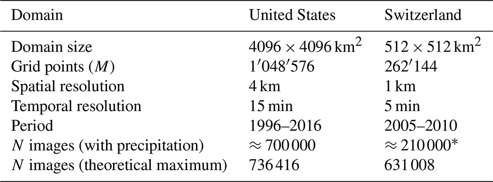
Inspired by Van Den Dool (1994), in Fig. 2 we estimated the minimum size of the radar archive needed to obtain sufficiently good analogues. We used the US dataset and targeted a spatial resolution of 4 km. The method analyses the dependence between the archive size and the smallest scaling distance r between real analogues, which is detected as a “crossing” point in the log–log plot of r vs. the correlation integral Cr (see Appendix D). More precisely, it consists of the following steps:
-
calculating the correlation dimension log–log plot for increasing archive sizes (Fig. 2a);
-
detecting the “crossing” points, i.e. the smallest scaling distance between real analogues for increasing archive sizes (squares in Fig. 2a);
-
selecting the largest correlation dimension (corresponding to the largest archive) and extrapolating the linear fit to obtain the correlation integral Cr associated with the desired resolution of r=4 km, i.e. (≈ radar observation error) (Fig. 2b); and
-
plotting the archive size vs. the Cr values of the crossing points and extrapolating the resulting fit to the desired to obtain the required archive size (Fig. 2c).
The point of crossing is detected on the log (r)−log (Cr) curve (Fig. 2a). It represents the point of maximum curvature between the steep scaling region in the middle of the curve and the flat region on its left (small radii). The flattening at small scales is due to the temporal correlation of the data, i.e. the consequence of estimating Cr on temporally correlated points (trajectories) rather than independent points (successive radar images are not real independent analogues). In contrast, the flattening on the right of the curve (large radii) occurs when the radii become larger than the subspace occupied by the attractor.
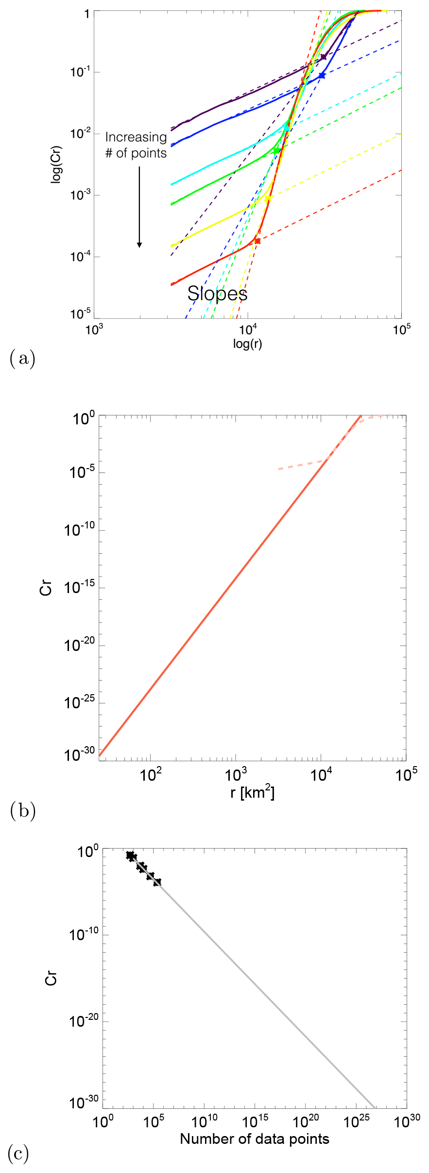
Figure 2Estimation of the theoretical size of the archive needed to find good radar analogues at 4 km resolution in the US. (a) Estimation of the correlation dimension and the point of crossing for increasing archive sizes (purple to red colours). (b) Estimation of the correlation dimension associated with a distance r=4. (c) Estimation of the archive size needed to reach C4 km from the points of crossing.
According to this analysis, for the number of points required to find good analogues is 3.41×1026, which corresponds to 9.73×10²¹ years. This result is based on the degrees of freedom of the image, which correspond to the number of pixels. Consequently, the only way of finding “good” analogues from the radar datasets is to reduce the degrees of freedom by defining a lower-dimensional phase space, which is the main objective of this paper.
2.3 From a high-dimensional dataset to a low-dimensional attractor
An archive of radar rainfall fields can be structured as a temporal sequence of images into a 2D array of size N×M:
where x1,2 is the rain rate at time index 1 and pixel index 2, N is the number of radar rainfall fields, and M is the number of grid points within a field. That is, each row is a flattened radar image. Hence, a sequence of rainfall fields represents a trajectory in an M-dimensional phase space, where for the Swiss domain and for the US domain.
A common approach to studying non-linear dynamical systems is to look at the evolution of trajectories in the phase space of governing variables (e.g. Lorenz, 1963; Abarbanel, 1997; Kantz and Schreiber, 2004). In this paper, the governing variables of the precipitation system are assumed to be the domain-scale statistics or principal components extracted from the high-dimensional radar archive.
The attractor represents the subspace attracting the trajectories of atmospheric states, in our case radar precipitation fields, starting from any initial condition within the phase space. Chaotic systems, i.e. systems with sensitive dependence on initial conditions, never cross the same trajectory again and generate “strange” attractors, which have a non-integer intrinsic dimension (fractal dimension). The Lorenz system and the atmosphere are two examples of strange attractors. The strange attractor of this study is the ensemble of possible states and trajectories derived from weather radar images that are consistent with the precipitation climatology of a given region.
2.4 Measuring error growth
As time passes, divergence between two initially close states in phase space increases, which is generally referred to as error growth (or spread growth). Idealized chaotic systems show three distinct regions of error growth: (1) an exponential growth at the start, (2) a power law growth, and (3) a region of saturation (loss of predictability); see for example Nicolis et al. (1995) and Atencia and Zawadzki (2017).
The established way of estimating the initial growth of errors, and therefore inferring the predictability of the system, is to compute Lyapunov exponents (e.g. Abarbanel, 1997; Kantz and Schreiber, 2004). Lyapunov exponents measure the rate of exponential error growth assuming an infinitesimally small initial error and an infinite lead time, while the maximum Lyapunov exponent is a measure of chaos strength (e.g. Lichtenberg and Lieberman, 1992). Unfortunately, such conditions are only met in idealized systems of equations (e.g. De Cruz et al., 2018). Such conditions are never observed with atmospheric measurements, whose analogue states have too high initial errors and measurement noise. Therefore, in this paper we looked for practical alternatives to Lyapunov exponents. Depending on the experiment, we computed as a function of lead time the
-
standard deviation (σ) of analogues around their mean
and
-
half the difference between the 84th and 16th percentiles of the distribution of analogue states:
which is analogous to s1 for a Gaussian distribution.
The analyses of the US attractor used only Eq. (2), while the ones of the Swiss attractor used both Eqs. (2) and (3). For simplicity, we refer to them as spread or error. The spread was further normalized by the sample climatological spread computed over the whole archive, so that saturation is reached around the value of 1 (comparable to selecting random analogues). The techniques to retrieve two (or more) close states are briefly described in the corresponding sections presenting the results.
2.5 Fractal properties of the attractor
Fractal properties of the attractor can give useful insights into its intrinsic dimensionality. In this paper, we combined the time-delay embedding and Grassberger–Procaccia correlation dimension methods (Grassberger and Procaccia, 1983).
The approach works by iteratively increasing the dimensionality of embedding space D (by time delay) until the estimated fractal dimension f (by Grassberger–Procaccia) converges to a finite value. When this point is reached, the attractor is completely unfolded, which may be evidence of a system driven by low-dimensional chaotic dynamics (and thus characterized by predictability). In contrast, the inability to converge towards a finite dimension would indicate the presence of unpredictable stochastic processes. Appendices C and D describe the time-delay and Grassberger–Procaccia methods and provide some references describing their known limitations.
3.1 Extracting phase space variables
There are many summary spatial and temporal statistics that can be extracted from precipitation fields and used as phase space variables, which we refer to here as domain-scale statistics. Keeping in mind that the attractor will be used for precipitation nowcasting or forecasting, we aim to extract variables that are relevant for those specific tasks. Several probabilistic precipitation nowcasting systems generate an ensemble nowcast by adding spatially and temporally correlated random perturbations to a deterministic extrapolation (e.g. Pegram and Clothier, 2001; Bowler et al., 2006; Berenguer et al., 2011; Atencia and Zawadzki, 2014; Nerini et al., 2017; Pulkkinen et al., 2019; Sideris et al., 2020). Such stochastic methods typically need to reproduce the following properties of precipitation fields.
-
The Fourier transform of the field (power spectrum), which is used to generate stochastic precipitation fields with a given spatial autocorrelation (e.g. Schertzer and Lovejoy, 1987; Pegram and Clothier, 2001)
-
The fraction of precipitation, which imposes the correct amount of zero precipitation (intermittency) on the spatially correlated field
-
The mean precipitation, which re-scales the non-zero values to reproduce the observed precipitation distribution
-
The temporal autocorrelation of precipitation fields, which is used by auto-regressive processes to make precipitation fields evolve over time
Note that it is also possible to condition the stochastic precipitation fields to the spatially localized fraction of precipitation, mean precipitation and Fourier transform (e.g. Nerini et al., 2017; Sideris et al., 2020).
A radially averaged 1D power spectrum (RAPS) can be derived from the 2D Fourier power spectrum (see Appendix A). The RAPS is one simple approach to check whether the precipitation field exhibits scale invariance within a given range of spatial scales, which is manifested in a power law relationship between the logarithm of the scale (spatial frequency) and the logarithm of the power spectrum:
where P is the Fourier power spectral density, k is the spatial frequency, and β is the slope of the power law, called the scaling exponent or spectral slope. β can be derived by ordinary least squares from the log–log plot of frequency against power. The Fourier transform can only account for the scaling of the second moment (variance), known as simple scaling. Multifractal approaches can handle the scaling of higher-order moments together with the intermittency of the field within a unified framework (e.g. Lovejoy and Schertzer, 2013).
Because rainfall rates often follow a log-normal distribution, it is more convenient to perform the Fourier transform on the reflectivity (Z) or rainfall rate (R) transformed in multiplicative units, i.e. and , respectively, where Z0=1 mm6 m−3 and R0=1 mm h−1. In addition, before performing the Fourier transform, we recommend setting all values below a chosen minimum threshold to the minimum threshold itself (e.g. mm−1, ∀i). This operation removes weak precipitation signals and smooths the resulting sharp corners of the rain–no-rain transition, which reduces the overestimation of power at high frequencies β (e.g. Nerini et al., 2017).
Several summary, spatial and temporal statistics were derived for the Swiss and US attractors, for instance:
-
WAR: wet area ratio (Pegram and Clothier, 2001). Percentage of wet (rainy) pixels over the radar composite domain (≥ 0.1 mm h−1).
-
Area coverage: number of wet pixels over the radar composite domain. This is similar to WAR.
-
IMF: image mean flux (Pegram and Clothier, 2001). Unconditional mean precipitation over the radar composite domain (including zeros). Note that this variable is correlated with WAR.
-
MM: marginal mean precipitation. Conditional mean precipitation (only wet pixels). Also referred to as conditional IMF. It can be computed in rain rate (mm h−1) or in linear reflectivity units Z.
-
β1 and β2: slopes of the spatial 1D RAPS. Two values are needed since spectra often show a scale break (e.g. Gires et al., 2011; Seed et al., 2013).
-
e: anisotropy of the precipitation field, as measured by the eccentricity of the spatial autocorrelation function. The latter is derived as , where am and aM are the minor and major axes of the fitted ellipse (derived by eigenvalue decomposition of the spatial covariance matrix).
-
Decorrelation time of precipitation fields, defined as the time when the temporal correlation falls below the value . The temporal correlation is derived by correlating precipitation fields at increasing time lags (e.g. Germann et al., 2006b).
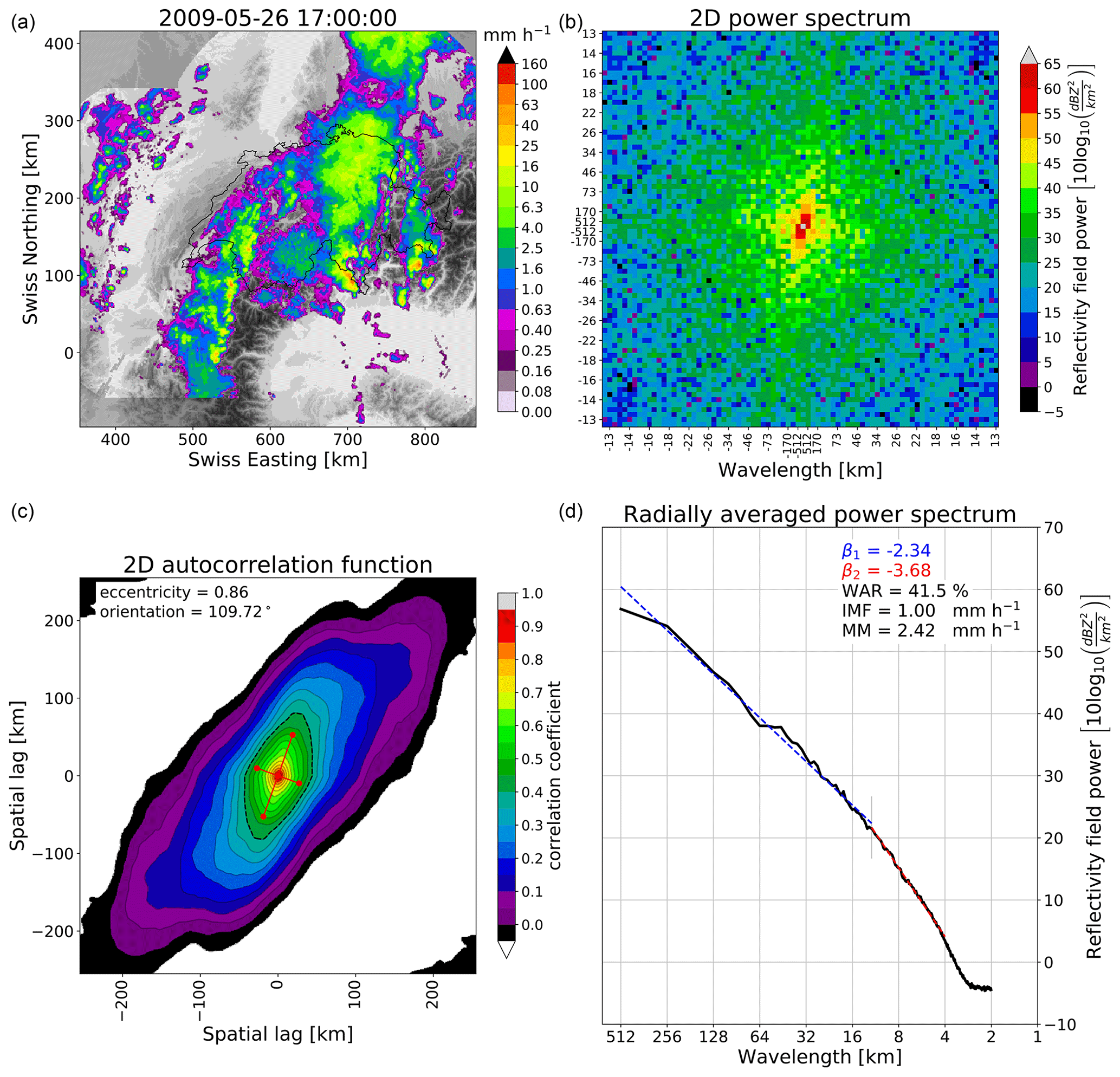
Figure 3Fourier analysis of the radar rainfall field at 17:00 UTC on 16 April 2016 in Switzerland. (a) Radar rainfall field overlaid on the digital elevation model (DEM). (b) Two-dimensional Fourier power spectrum rotated by 90° (zoom for wavelengths larger than 13 km). (c) Spatial autocorrelation function. (d) Radially averaged 1D power spectrum in a log–log plot, together with the estimated spectral slopes β1, β2, WAR, IMF and MM statistics. See other examples in Nerini et al. (2017).
Figure 3 shows an example of a composite radar rainfall field at 17:00 UTC on 17 April 2016 in Switzerland, with the corresponding 2D power spectrum, 1D RAPS and 2D autocorrelation function (computed by inverse fast Fourier transform (FFT) of the 2D spectrum; see Appendix A). The RAPS exhibits the typical power law scaling behaviour of precipitation fields. The scaling break occurs around the 20 km wavelength, in agreement with other studies (Seed, 2003; Seed et al., 2013).
3.2 Phase space trajectories
Figure 4 represents the density of points (trajectories) of a 4D US precipitation attractor that was constructed using the following phase space variables: decorrelation time, eccentricity, area coverage and marginal mean. These variables were selected to be independent of each other, although we can still notice some interesting dependencies between variables, for example the increase in decorrelation time with increasing rainfall area (top left) and increasing eccentricity (top centre). This may indicate that precipitation fields that are less widespread and more isotropic, for example isolated convective cells, are less predictable (according to the decorrelation time), while more organized frontal precipitation with large-scale anisotropy is more predictable. The density plot of decorrelation time vs. marginal mean also has a peculiar shape. The decorrelation time increases until MM ≈ 23 dBZ but then starts decreasing. This could be attributed again to the lower predictability of isolated intense convective cells compared to stratiform precipitation. Moreover, the larger variance of convective precipitation reduces the decorrelation time.
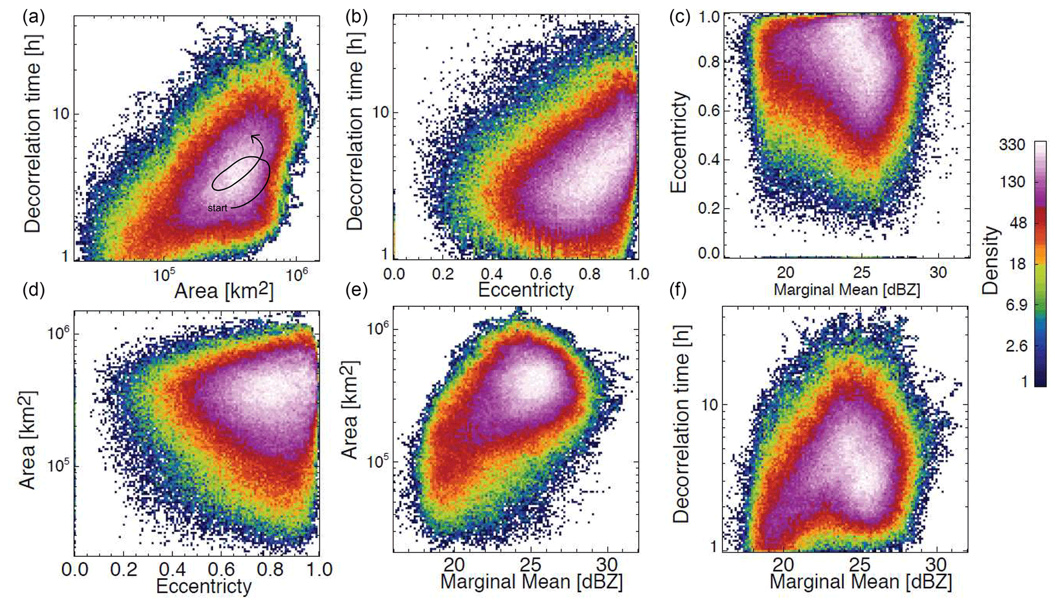
Figure 4US precipitation attractor. It is represented by 2D histograms (counts) using as phase space variables the marginal mean precipitation (MM), area coverage, decorrelation time, and eccentricity of composite radar precipitation fields. For illustrative purposes, panel (a) includes a dummy trajectory representing a sequence of radar fields within the attractor.
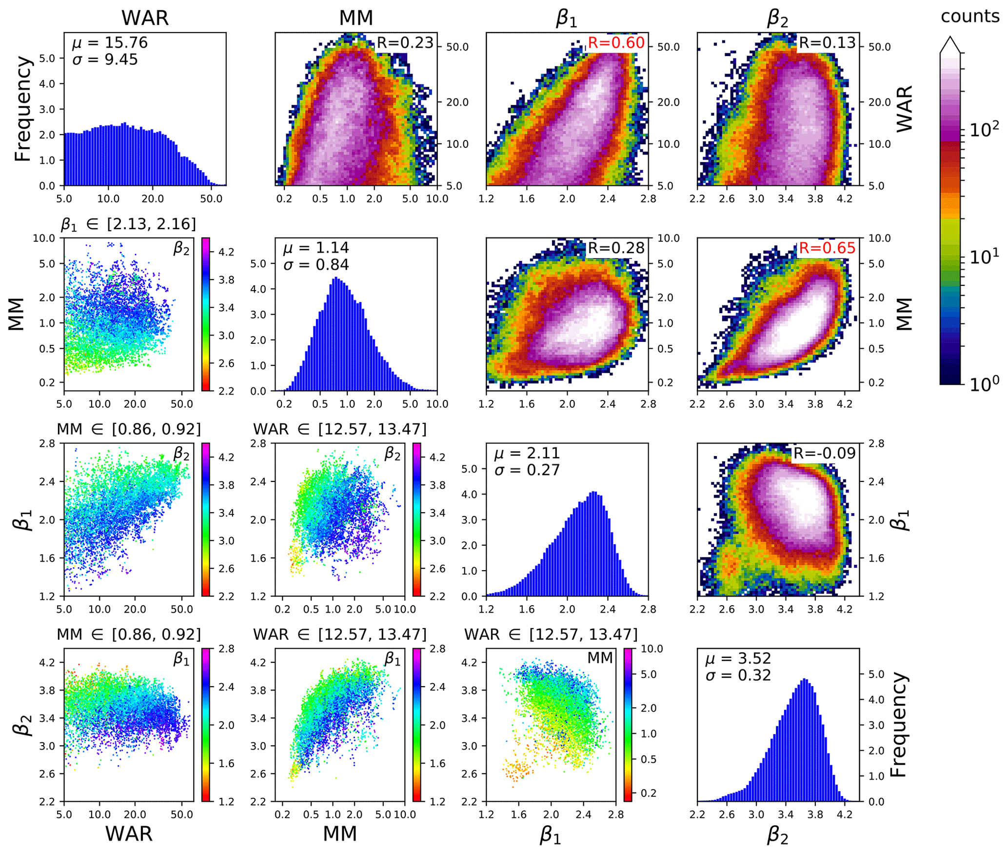
Figure 5Swiss 4D precipitation attractor. The phase space variables are the marginal mean precipitation, the wet area ratio, and the two spectral slopes of the RAPS (β1, β2). MM and WAR are shown on the log scale to account for the asymmetry of the distribution.
Figure 5 visualizes a Swiss 4D precipitation attractor embedded in the phase space composed of WAR, MM, β1 and β2. These variables are different from the ones used in the US because in Switzerland we were developing a nowcasting system depending on those four variables, while in Canada we were doing a more general-purpose study. The attractor is constructed using all the rainfall fields from 2005 to 2010 that have a WAR ≥ 5 % and where the fitting of the spectral slopes is of good quality, i.e. when the correlation coefficient of the linear regression is above 0.95 (for both β1 and β2). These criteria are met by 209 715 rainfall fields (33 % of the total number of images). The figure panels are organized in a 4×4 matrix, where each row (column) represents one phase space variable.
The four plots on the diagonal show the univariate histograms of the four variables and the corresponding summary statistics (mean and standard deviation).
The subplots in the upper triangular part of the matrix show the 2D histograms describing the density of points for all combinations of phase space variables (same as Fig. 4). In the upper right part of each subplot, there is the correlation coefficient between the two variables. Interesting correlations can be noticed between WAR vs. β1 and MM vs. β2. The first reveals that increasing the rainfall fraction over the radar domain increases the power at large spatial scales. The second highlights the convective cases (high MM), which increase the power at wavelengths of ≈ 10–20 km and thus the value of β2. In the context of spatial scaling analysis, the density plot of β1 vs. β2 is quite interesting as it summarizes the average scaling behaviour of Alpine radar rainfall fields over many years, i.e. and . Such findings are relevant in the context of stochastic rainfall simulation since β determines the type of approach needed, which depends on whether β is below or above the dimension of the field (β>2): see e.g. Menabde (1998).
The subplots in the lower triangular part of the matrix are a simplified representation of surfaces of section (e.g. Sideris, 2006), also known as Poincaré maps (e.g. Lichtenberg and Lieberman, 1992). In practice, they represent a cross section through the attractor. They are obtained by plotting only the points whose values fall in an interval around the 50th percentile of a given variable. For example, the subplot in row 2 and column 1 in Fig. 5 only shows the points in the interval 2.13–2.16 for β1. The x axis and y axis are the variables WAR and MM, respectively. Finally, the points are coloured according to the remaining fourth variable (β2). This type of representation helps analyse the dependencies between variables in the 4D space, e.g. the clear increase in β2 when increasing MM (row 3, column 2) or the increase in β2 with decreasing β1 (row 3, column 1), which was not visible from the density plot (row 3, column 4).
These graphical illustrations represent a first useful insight into the attractor. For example, it is possible to distinguish between the stratiform and convective precipitation systems using combinations of phase space variables, in particular the eccentricity, spectral slopes and decorrelation time.
3.3 Scaling properties
The domain-scale precipitation attractor provides additional insight into the origin of the spatial scaling break in the Fourier power spectrum. The scaling break was already noticed by previous studies, e.g. Gires et al. (2011) and Seed et al. (2013). The results of the latter provide hints that the scaling break is related to the presence of convective precipitation.
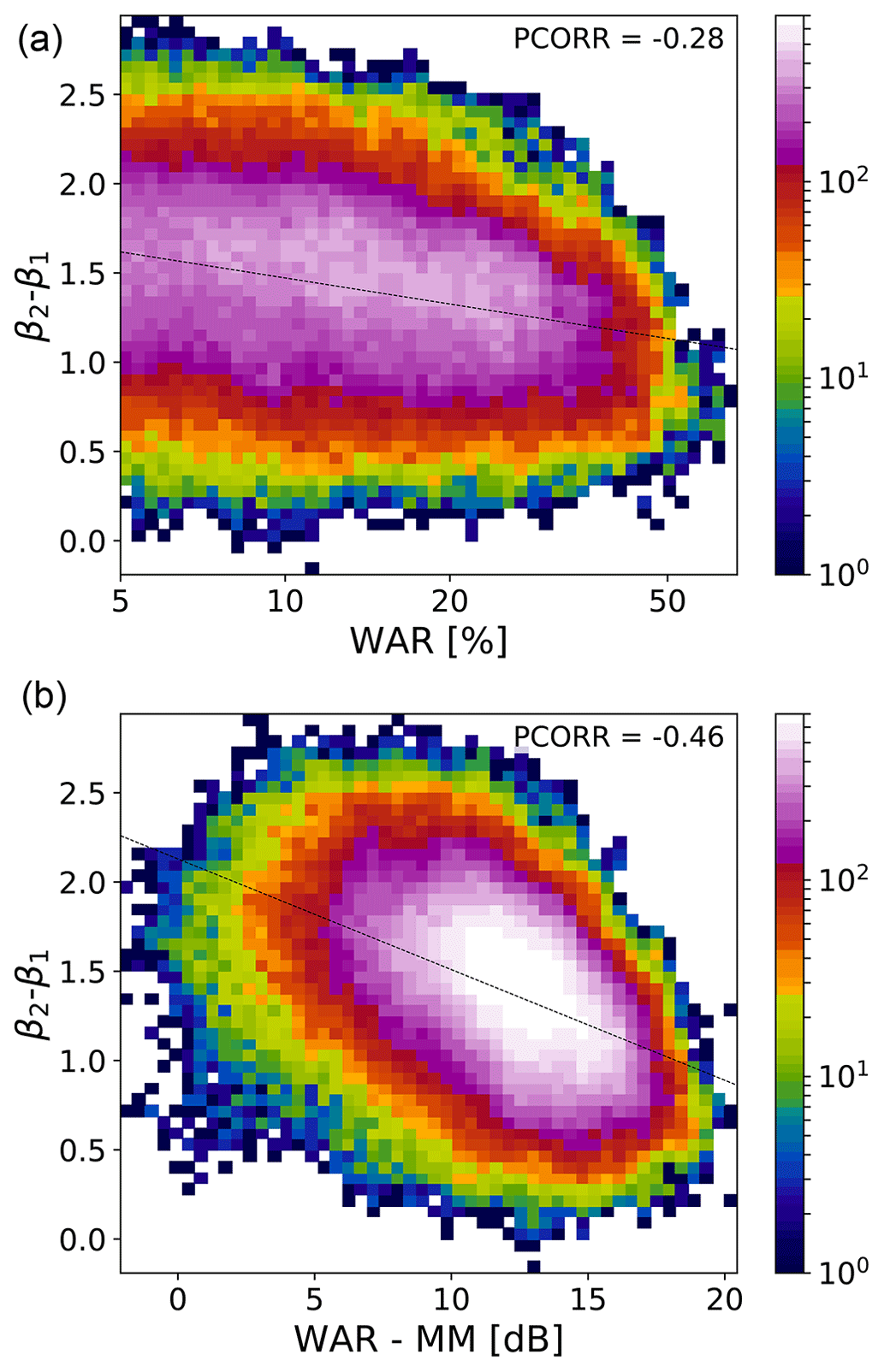
Figure 6Analysis of scaling break magnitude (β2−β1) w.r.t. the (normalized) rainfall fraction. Two-dimensional histogram of (a) β2−β1 vs. WAR (%, log scale) and (b) β2−β1 vs. WAR-MM (dB). If , there is no scaling break.
Figure 6 shows the relationship between the magnitude of the scaling break, defined as β2−β1, with the rainfall fraction (WAR). Figure 6a shows that the scaling break magnitude tends to decrease for increasing WAR values. This dependence is enhanced further when normalizing the WAR by the MM, which leads to a correlation of almost −0.5 (Fig. 6b). The variable WAR−MM(dB) is an effective way of describing whether the precipitation field is more of a stratiform or convective type. The scaling break is more pronounced when intense precipitation is concentrated in a few areas (small WAR and high MM). In contrast, widespread low-intensity precipitation (high WAR and low MM) reduces the magnitude of the scaling break.
This brief analysis sheds new light on the origin of the scaling break in power spectra of precipitation fields, which is helpful for designing stochastic models (e.g. Seed et al., 2013). For instance, one single spectral slope would be sufficient to simulate stratiform precipitation fields, while two spectral slopes are necessary to simulate convective precipitation fields. This also means that convective precipitation fields exhibit a weaker scaling behaviour than large-scale stratiform precipitation systems. It is not surprising then that nowcasting of thunderstorms is done by cell-tracking techniques rather than scaling approaches.
3.4 Fractal properties
To estimate the fractal dimension of the attractor, we applied the time-delay embedding technique and correlation dimension method to each time series of phase space variables.
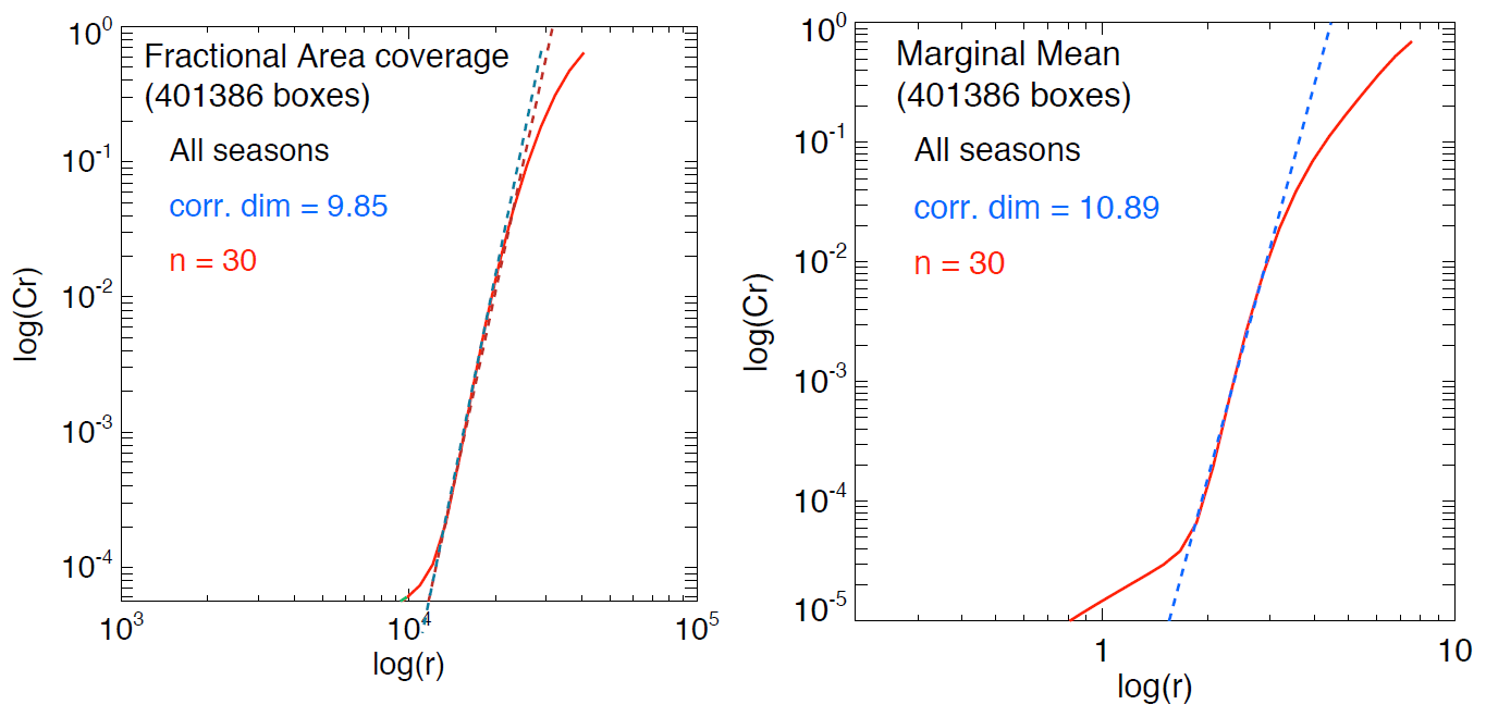
Figure 7Correlation dimension estimation using the Grassberger–Procaccia algorithm and time-delay embedding on the variables fractional area coverage and marginal mean on the US attractor. log (r) is the logarithm of the radius containing the points, while log (Cr) is the corresponding (normalized) correlation integral, i.e. the average number of points found within that radius.
Figure 7 shows the estimated fractal dimension of the US precipitation attractor for the fractional area coverage and the marginal mean time series. For an embedding space of D=30 variables, the correlation dimensions stabilize to f=9.85 for the fractional area and f=10.89 for the marginal mean. However, due to known limitations of the Grassberger–Procaccia algorithm, we cannot claim that such finite correlation dimensions are evidence of a low-dimensional chaotic system (see the references in Appendix D).
Instead of re-doing the same analysis with the Swiss attractor, in Sect. 4.6 we will exploit the PCA framework to estimate scale-dependent fractal dimensions, which can be compared in relative terms rather than interpreted in absolute terms.
3.5 Growth of errors
Once the phase space is defined, we can study the intrinsic predictability of states starting from close initial conditions, the so-called analogues. We retrieved the analogues by dividing each variable of the attractor into 10 intervals (from minimum to maximum values). More precisely, a 1D attractor has 10 intervals, a 2D attractor 100 squares, a 3D attractor 1000 cubes, a 4D attractor 10 000 hypercubes, and so on. The points that fall within the same hypercube are considered analogues. Cubes with less than 20 analogues were discarded.
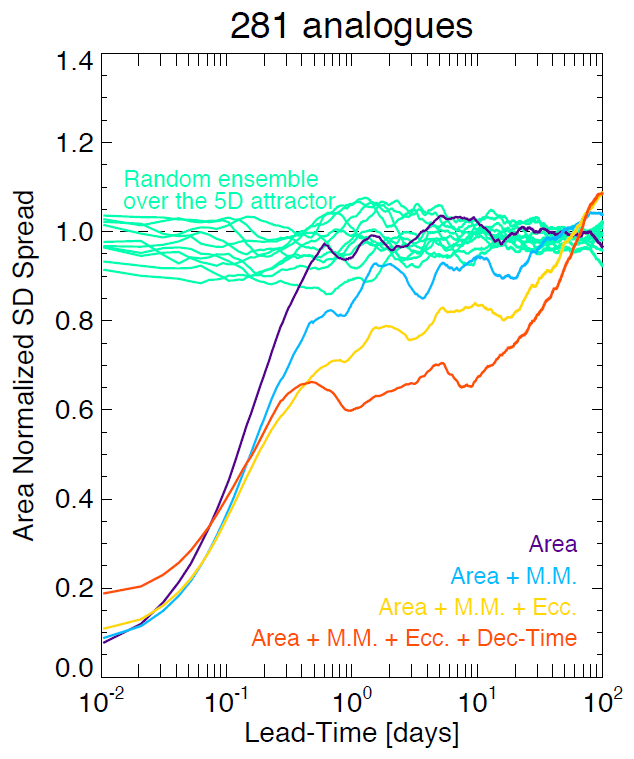
Figure 8Average standard deviation of analogues in the US attractor as a function of lead time for phase spaces of increasing dimensionality. The x axis is logarithmic, while the y axis is linear to highlight the longer-range predictability. The spread is computed according to Eq. (2).
Figure 8 shows the average growth of the standard deviation of retrieved analogues (spread) on the US attractor. The analyses are done by incrementally adding phase space variables starting from the rainfall area. The error growth (spread) is characterized by the following stages:
-
≈ 0–1 h: initial slow exponential growth (nowcasting range);
-
≈ 1–6 h: fast power law growth (from nowcasting to short range);
-
≈ 6 h–20 d: slow growth again (from short range to medium range); and
-
20 d: saturation stage (loss of predictability).
The reason for the slow error growth at 0–1 h is mostly unknown. It might be related to some radar data processing steps, in particular those that introduce smoothness in the precipitation field, which leads to overestimation of the predictability at the smallest scales. The rapid error growth at 1–6 h is attributed to the low predictability of precipitation growth and decay, especially in convective systems. The slower error growth at 6 h–20 d can be explained by the more predictable translation of synoptic-scale features across the continental US. Note that saturation already occurs after ≈ 6 h when using the variable area alone. Adding phase space variables improves predictability in three ways: (1) by reducing the rate of error growth in the first 2–3 h, (2) by reducing the spread in the range ≈ 6 h–20 d, and (3) by extending the saturation stage by several days. However, the 4D attractor has a larger initial error (≈0.2), which reflects the difficulty in finding states that are similar in all variables simultaneously. Despite the initial disadvantage, the 4D attractor shows better medium- and long-range predictability.
These promising results show that there is unexpected intrinsic predictability of precipitation if the appropriate phase space variables are chosen. Given the substantial improvement of predictability in the range ≈ 6 h–20 d, it would also be interesting to study whether analogues can help extend the range of NWP models (e.g. by blending probabilities).
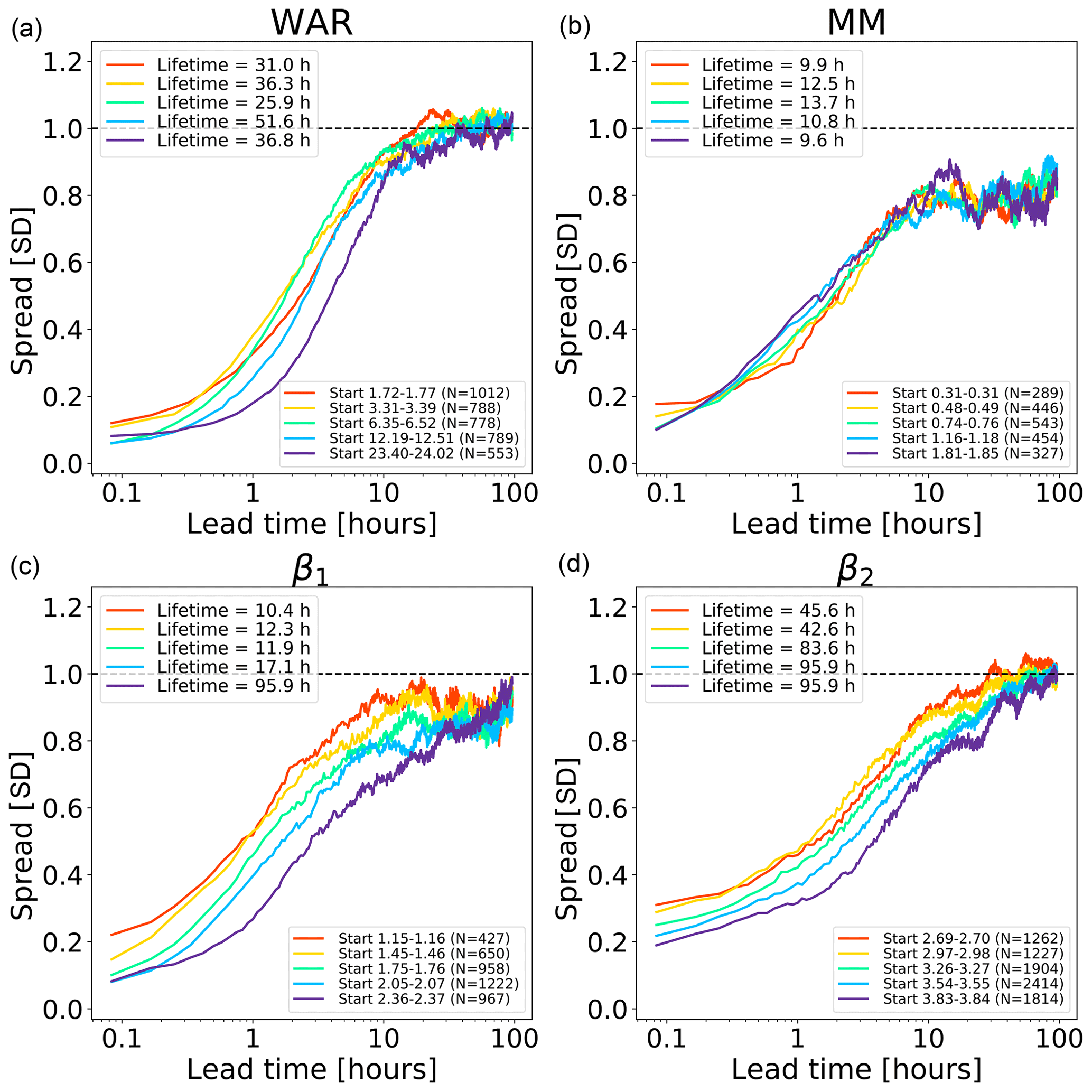
Figure 9Error growth of an ensemble of analogues starting from different initial conditions on the Swiss attractor. The upper end of the x axis corresponds to a lead time of 96 h (4 d). The number of analogues N is shown in the figure legends. The x axis is logarithmic, while the y axis is linear to highlight the longer-range predictability. The spread is computed according to Eq. (2).
Another interesting experiment is to analyse the local variability of predictability within the attractor. This could inform about the dependence of intrinsic predictability on initial location within the attractor (e.g. Li and Ding, 2011).
In order to simplify the task, here we only consider 1D trajectories, i.e. time series of individual phase space variables, hereafter extracted from the Swiss attractor. The small interval defining the initial conditions is selected by regularly spaced values between the 20th and 90th quantiles of each phase space variable. At each quantile, we select all the analogues that are within a small neighbourhood and that are at least 1 h from each other (to reduce dependence among analogues).
Figure 9 shows the growth of spread of an ensemble of analogue time series starting under close initial conditions. The reported lifetime characterizes the lead time after which the spread reaches saturation. It is estimated by fitting a non-parametric kernel ridge regression to the data points and by taking the value at which the first derivative approaches zero. Such estimations are only approximate as they depend on the convergence criterion chosen. Depending on the phase space variable and the initial conditions, we obtain different lifetime estimations, which reflects the predictability dependence on the initial conditions. The saturation times vary between 10 h and more than 90 h, which are shorter than those obtained in the US (Fig. 8). The shorter predictability over the Alpine region is mainly attributed to the smaller domain size (64 times smaller than the US), where it is not possible to observe the full precipitation extent and lifecycle of extra-tropical cyclones. By comparing Figs. 8 and 9, we notice that the regions of fast error growth in the range 1–6 h correspond quite well, although the Swiss attractor shows a less clear breaking point at around 6 h compared to the US.
Most curves in the Swiss attractor miss the initial slow error growth observed in the US attractor (Fig. 8). They also start from quite different initial values, depending on the variable chosen. For example, β2 has rather high initial errors, which indicates that it has a larger intrinsic variability (noise). Despite the larger initial error, β2 seems to take longer than β1 to saturate (from several hours to days, depending on the chosen saturation thresholds). Despite flattening considerably after 5–6 h, the MM does not reach saturation completely.
These findings provide some useful information on the predictability that could be obtained by extrapolation nowcasts. In fact, the smaller size of the Swiss domain (as compared with the US) imposes a shorter limit of predictability, which could only be extended by enlarging the domain or by forecasting the evolution of domain-scale statistics.
Appendix E shows various experiments to analyse the sensitivity of predictability estimations to the scaling of the time and error axes as well as the use of different spread metrics.
4.1 Extracting phase space variables
Domain-scale statistics are unable to describe the spatial distribution of precipitation, unless they are computed locally (e.g. Sideris et al., 2020). A possible solution is to use PCA. PCA is a method of compressing the information contained in a dataset of correlated variables, which has been extensively used in atmospheric and climate science (e.g. Lorenz, 1956; Richman, 1986; Jolliffe, 2002; Schiemann et al., 2010; Foresti et al., 2015; Nerini et al., 2019). The procedure consists of finding an orthogonal transformation that linearly combines the variables to form a set of uncorrelated variables sorted by explained variance, which are called principal components.
The variables of the precipitation data matrix (Eq. 1) are strongly correlated since each column represents a time series of precipitation for 1 pixel of the radar image. The so-called S-mode PCA exploits the spatial dependence to compress the information contained in the radar archive into a small set of principal components, which are used here as phase space variables. The lower-dimensional phase space is obtained by projecting the data matrix as follows:
where UM,D is the truncated matrix of eigenvectors (projection matrix), XN,M is the original data matrix (Eq. 1), and YN,D is the (truncated) matrix of principal component scores (projected matrix), which contains the coordinates of radar images in the phase space. For more details on the PCA implementation, we refer to Appendix B.
Due to the too large size of the US dataset, the radar fields were upscaled to a resolution of 64×64 km2 pixels using a Haar wavelet transform before applying PCA. This pre-processing step only marginally affects the search for analogues as we are interested in similarity at synoptic scales. We did not attempt to upscale the Swiss radar domain to the resolution of 64×64 km2 pixels as this would have given an 8×8 radar image, too small to provide a meaningful comparison to the US dataset.
4.2 Plotting phase space variables
Figure 10 shows the fields of eigenvectors computed from the US radar archive (1996–2016). The first eigenvector (ϵ 0) explains only 4.8 % of the total variance and is characterized by positive values in the middle of the domain. It was found that the first principal component (PC), associated with the first eigenvector, is strongly correlated with the field IMF (e.g. Foresti et al., 2015). Radar images with precipitation located in this region will also have correspondingly high PC0 scores. All other eigenvectors can be interpreted in a similar way. For instance, the second (ϵ 1) and third (ϵ 2) eigenvectors discriminate precipitation patterns in the west–east and north–south directions, respectively. Therefore, a precipitation system moving from west to east will show an increase in PC0 followed by an increase in PC1. Finally, eigenvectors exhibit a characteristic sorting by spatial scale.
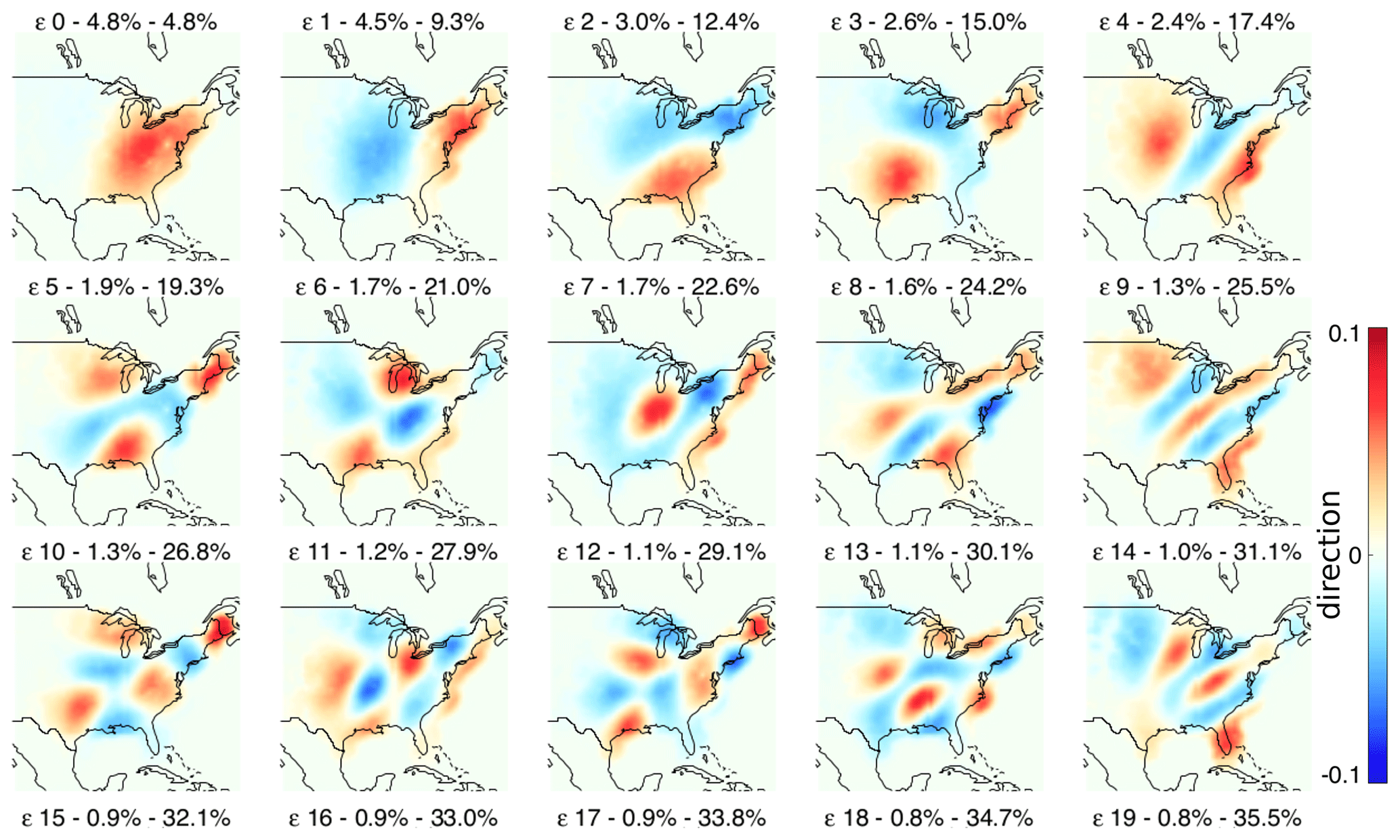
Figure 10Eigenvectors (loadings) extracted by PCA from the US radar archive.
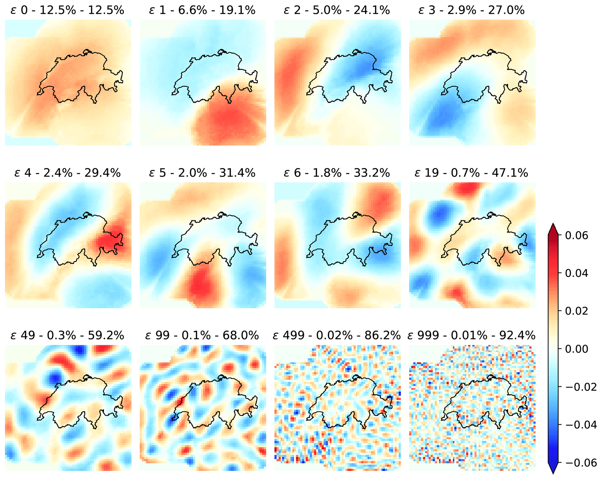
Figure 11Eigenvectors (loadings) extracted by PCA from the Swiss radar archive.
Figure 11 shows the eigenvectors of the Swiss radar dataset (2005–2010), which also shows the characteristic sorting by the spatial scale. The domain is much smaller compared with the US, but similar patterns can be observed, for example the tendency of the first eigenvector to have high values in the middle of the domain and the dipole shape of the second and third eigenvectors oriented in the north–south and east–west directions.
These shapes not only highlight the most common precipitation regimes but are also influenced by the rectangular shape of the domain and the orthogonality constraints of PCA. These dipole effects are known in the literature as Buell patterns and can complicate the meteorological interpretation of principal components (e.g. Richman, 1986).
In an attempt to improve their interpretation, we implemented a varimax rotation of the principal components (e.g. Richman, 1986), which were truncated at different thresholds of the cumulative explained variance (before rotation). The rotated eigenvectors highlighted some parts of the domain (with values close to zero elsewhere) and lost the sorting by the spatial scale. As we did not find these results informative, they were not included in the paper.
Figure 11 also shows a few eigenvector fields for higher PC numbers (50, 100, 500 and 1000). After 500 components the eigenvectors become more noisy and describe very small-scale precipitation features. Note that even after 500 eigenvectors there is still almost 15 % unexplained variance.
PCA explains more variance with fewer components in the Swiss dataset. For instance, with 20 components the cumulative explained variances are 47.1 % and 35.5 % for the Swiss and US domains, respectively. This can be attributed to the smaller Swiss dataset but also to the more frequent orographic precipitation events related to the presence of the Alps, which determines more predictable spatial patterns on the upwind and downwind sides of the Alpine chain.
A common pattern for both Swiss and US attractors is that PCA decomposes the dataset into a set of eigenvectors that represent decreasing spatial scales, similarly to what is obtained with a Fourier-based cascade decomposition of precipitation fields (Seed, 2003; Seed et al., 2013). This phenomenon is detailed further in the next section.
4.3 PCA vs. Fourier analysis
The sinusoidal patterns of eigenvector fields are an outcome of the Toeplitz-like nature of the covariance matrix of spatially correlated fields, whose eigenvectors represent sines and cosines of increasing frequencies. More precisely, for a stationary process the sinusoidal basis functions of the Fourier transform form a valid principal component basis, where the variance of each component represents the power spectrum (e.g. Simoncelli and Olshausen, 2001).
PCA derives the basis functions by decomposing an empirical covariance matrix. This may explain why in atmospheric science the principal components are referred to as empirical orthogonal functions (EOFs Lorenz, 1956; Richman, 1986). Instead, Fourier analysis assumes the orthogonal basis to be composed of sines and cosines, which is imposed prior to the analysis. Such assumptions simplify the use of Fourier analysis, which can also be applied to a single radar image. Instead, PCA needs an archive of radar images to derive the orthogonal basis. We find here again the inductive vs. deductive dichotomy as in the definition of the phase space variables.
The similarity between PCA and Fourier decomposition creates interesting links to the cascade decomposition used in the Short-Term Ensemble Prediction System (STEPS Seed, 2003; Bowler et al., 2006). In STEPS, the FFT is used to decompose and simulate precipitation fields within a multiplicative cascade framework, where each level represents precipitation features at different spatial scales.
Inspired by the relation to the cascade decomposition, Nerini et al. (2019) used PCA to blend radar ensemble nowcasts with NWP ensembles in a reduced space. An interesting future development arising from these findings could be to stochastically simulate precipitation fields in the space of principal components, for example by extending the method of Link et al. (2019).
4.4 Phase space trajectories
Figure 12 shows the trajectories of US radar composite images in the space of the first PCs. For this experiment, PCA was only applied to 23 manually selected similar events to better understand its inner workings. The selection included well-organized precipitation systems moving across the continental US from west to east.
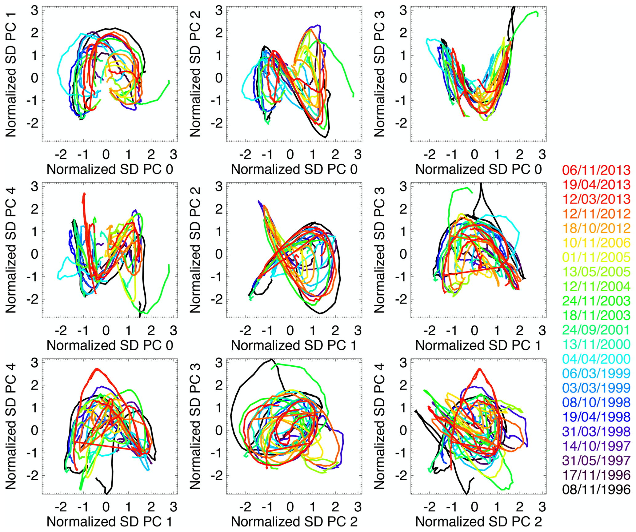
Figure 12Trajectories of similar radar image sequences over the US in the space of standardized principal components. The dates of the 23 similar precipitation events are displayed on the right.
An interesting observation is that PC trajectories define quasi-regular trajectories, which result from the translation of precipitation systems from west to east. The most regular and illustrative PC shapes are found in the three sub-panels located as follows (row, column): (1,2), (1,3) and (2,2). The one at (1,2) has a faint resemblance to the Lorenz attractor, which is only a fortunate coincidence.
This behaviour is not surprising: as explained in Sect. 4.2, the second (west–east) and third (north–south) principal components describe the general location of the precipitation system within the domain. The faster the precipitation system moves e.g. from west to east, the faster the trajectory is along the second principal component.
4.5 Scaling properties
The sorting of eigenvectors by spatial scale observed in Sect. 4.2 is corroborated by plotting the explained and cumulative variance vs. the ordinal principal component number in log–log scale, as shown in Fig. 13. Indeed, the explained variance draws a clear straight line (power law), similar to those obtained from Fourier-based scaling analyses (see e.g. Fig. 3).
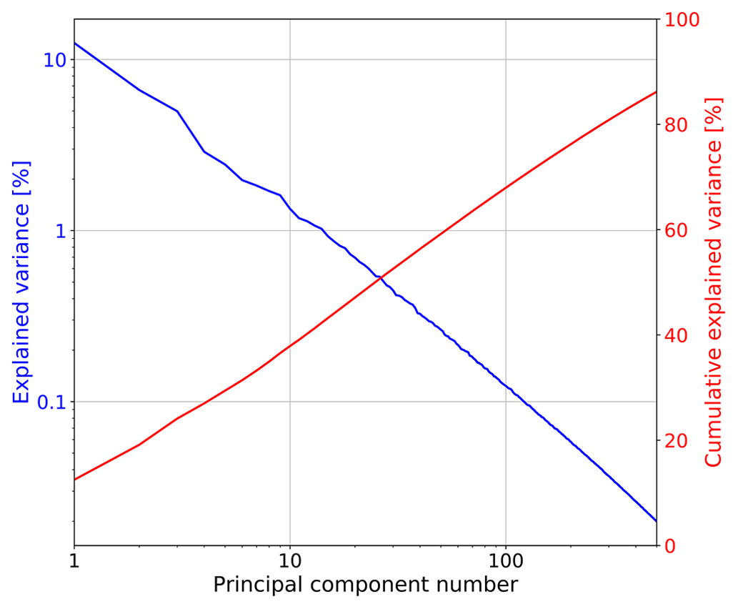
Figure 13Explained variance and cumulative explained variance vs. the principal component number from the Swiss PCA.
The slow increase in cumulative explained variance does not allow us to define a clear cutoff level to truncate the principal components. These results do not leave a lot of optimism concerning the definition of a low-dimensional attractor for precipitation based on PCA. Instead, they point towards a stochastic approach for precipitation analysis and simulation.
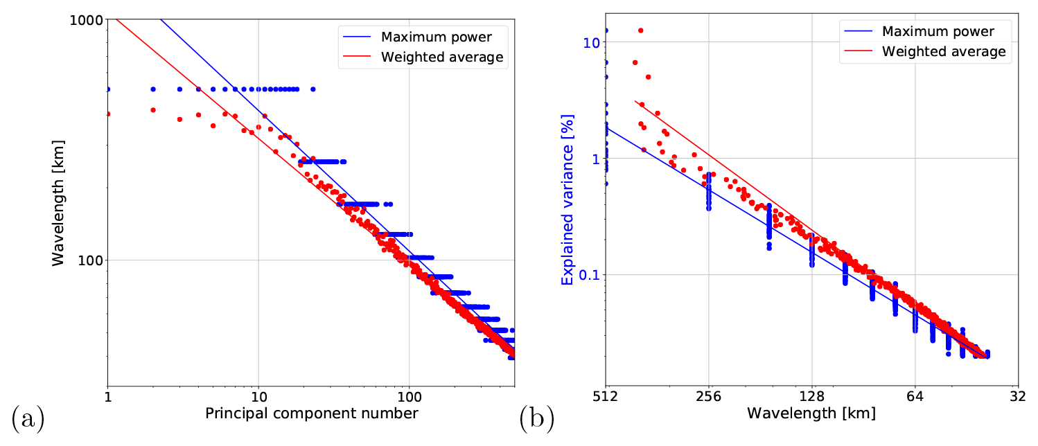
Figure 14Derivation of spatial wavelength from PC number. (a) Wavelength vs. PC number. (b) Explained variance vs. wavelength (spatial frequency), which can be interpreted as a Fourier power spectrum.
One way of establishing an empirical relation to Fourier-based scaling analysis is to convert the ordinal PC numbers of Fig. 13 into the corresponding spatial scales γ, which are represented by spatial wavelengths . For this task, we developed the following methodology (see Fig. 14).
- 1.
Compute the 2D Fourier spectra of the eigenvector fields (e.g. of Fig. 11).
- 2.
Derive the 1D RAPS from the 2D spectra.
- 3.
Estimate the most representative wavelength λ from each 1D spectrum. We tested two methods:
- a.
the maximum power method, which returns the wavelength with maximum power; and
- b.
the weighted average method, which computes an average of wavelengths weighted by power.
- a.
- 4.
Plot the obtained wavelength against PC number in log–log scale (Fig. 14a).
- 5.
Replace the PC number with the corresponding wavelength and plot it against the explained variance from Fig. 13 (Fig. 14b).
Figure 14 demonstrates the existence of a power law relationship between the wavelength and both the PC number and explained variance. The results obtained with the maximum power and weighted average methods are quite similar, despite some deviations above the 300 km wavelength (due to wavelengths larger than the domain size).
These findings point out that there is no universal relationship that maps the ordinal PC number to the spatial scale, as the latter depends on the covariance matrix of a given dataset. However, the method proposed above offers a simple and effective way of revealing the spatial scale represented by a given eigenvector.
4.6 Fractal properties
Figure 15 shows an experiment to separate the predictable and unpredictable precipitation scales using the Swiss attractor. The assumption is that the time series of PCs representing large-scale features converge to a lower correlation dimension than the ones representing the more “stochastic” small scales. Note that a similar experiment was also done by Alberti et al. (2023) using multivariate empirical-mode decomposition on the Lorenz system.
Figure 15a shows the temporal autocorrelation functions (ACFs) of a selection of principal component time series. Rather than computing a single ACF for the whole time series (6 years of PC values), we computed it for each precipitation event (separated by a sufficiently long period without precipitation). This step was needed because the (long) periods without precipitation were artificially increasing the temporal autocorrelation. As expected, there is a decrease in the decorrelation time for increasing PCs. The very high correlations in the first hour, especially visible for PC1, could be related to the slow error growth in the 0–1 h range already observed in the US attractor (see Fig. 8). However, they might also be explained by artifacts introduced by PCA, which artificially increase the smoothness of time series.
The first minimum of the ACF was used as time delay τ by the time-delay embedding method to estimate the associated correlation dimension of each PC time series (see Fig. 15b). The results show that all the time series converge towards a finite correlation dimension, which grows from 2 to 4–5 when going from the 1st to 100th PCs. Only the last PC does not converge. These results highlight the expected underestimation of the correlation dimension of the Grassberger–Procaccia method (Schertzer et al., 2001).
A major difficulty that we encountered in applying time-delay embedding is related to the short duration of precipitation events compared with the time delay τ. In fact, if we consider a normal precipitation event lasting 24 h (over the Swiss domain) and τ=4 h, the maximum dimensionality of the embedding space is . Adding more variables will only include radar images with no precipitation in the time series and form a fixed point in the attractor, which adversely affects the estimation of the fractal dimension. This constraint is clearly visible in Fig. 15c, which shows the number of samples available to compute the correlation dimension as a function of the embedding dimension and PC number. One way to reduce this effect is by choosing larger domains to increase the probability of there being precipitation somewhere.
Finally, even though the fractal dimension estimates in this paper cannot be interpreted in absolute terms, they can be interpreted in relative terms. That is, lower PCs exhibit stronger chaotic behaviour than larger PCs, which have a more stochastic behaviour.
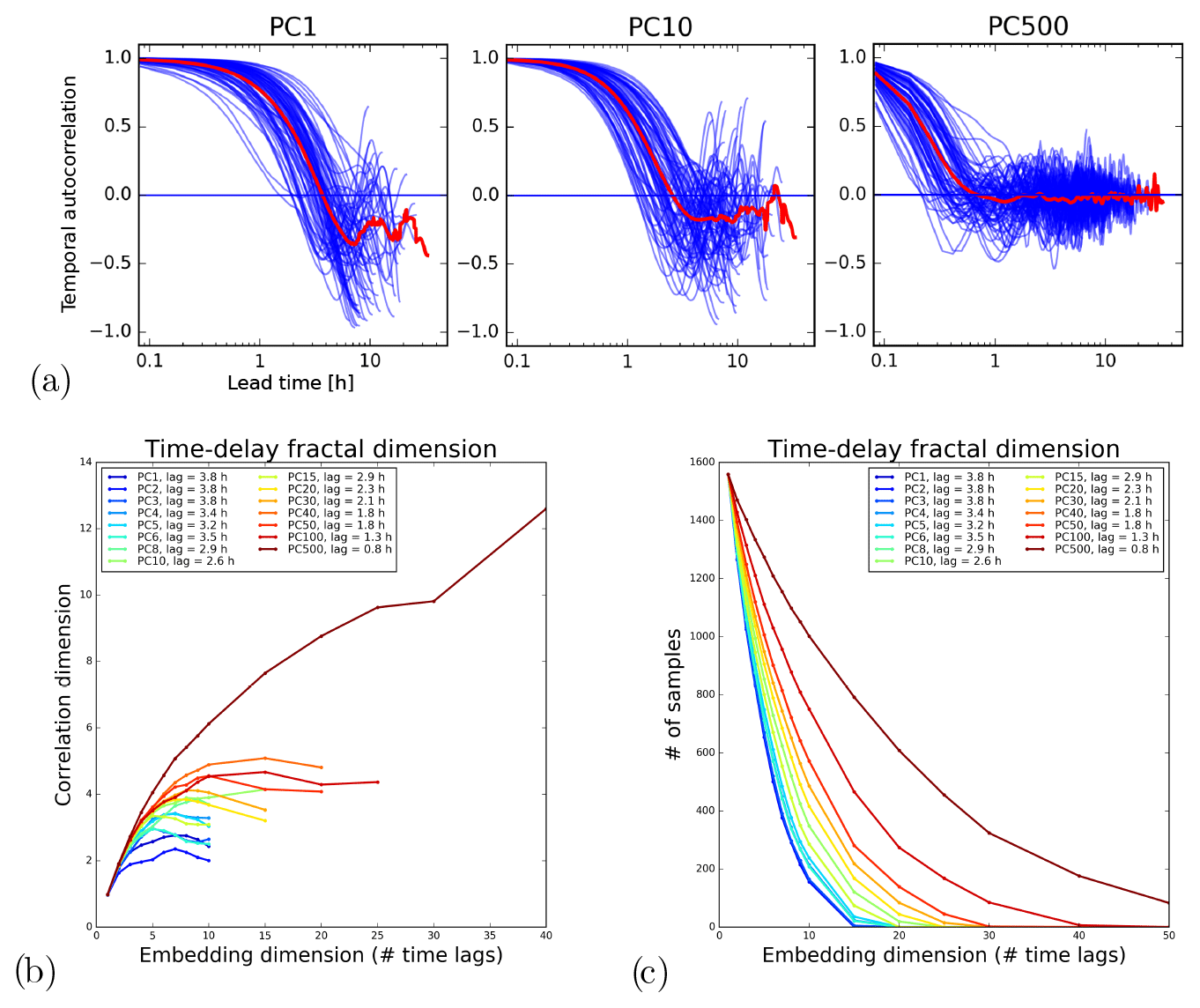
Figure 15Correlation dimension analysis of principal component time series on the Swiss attractor. (a) Temporal autocorrelation functions of the PC time series for different precipitation events (blue) and the average ACF (red). (b) Correlation dimension vs. embedding dimension for different PCs. (c) Number of samples available for the estimation.
4.7 Growth of errors
Figure 16 shows the forecast accuracy obtained by analogues for different PCA configurations and normalization of data. Each PCA configuration comprises a combination of Wavx, PCAx and rotation parameters.
-
Wav1: before PCA, subtract the mean from data columns.
-
Wav2: before PCA, subtract the mean and divide the data columns by standard deviation.
-
PCA1: after PCA, use raw PC scores.
-
PCA2: after PCA, subtract the mean and divide the PC scores by their standard deviation.
-
PCA3: after PCA, weight each PC score by the explained variance.
-
Rotation (varimax): yes/no.
-
Random: random selection of analogues.
The forecast quality of analogues was measured by three continuous verification scores, i.e. mean absolute deviation (MAD), root-mean-square error (RMSE), Pearson's correlation, one categorical score (critical success index, CSI) and two probabilistic scores, i.e. the area under the ROC curve and the Brier score at the 1 dBZ threshold. The verification was done using 50 precipitation events in the US. For each of the 50 events, 25 analogues were selected based on the smallest Euclidean distance in PC space and forcing them to be at least 16 h from each other (for temporal independence). A 90 % threshold of the cumulative explained variance was used to define the dimensionality of the phase space.
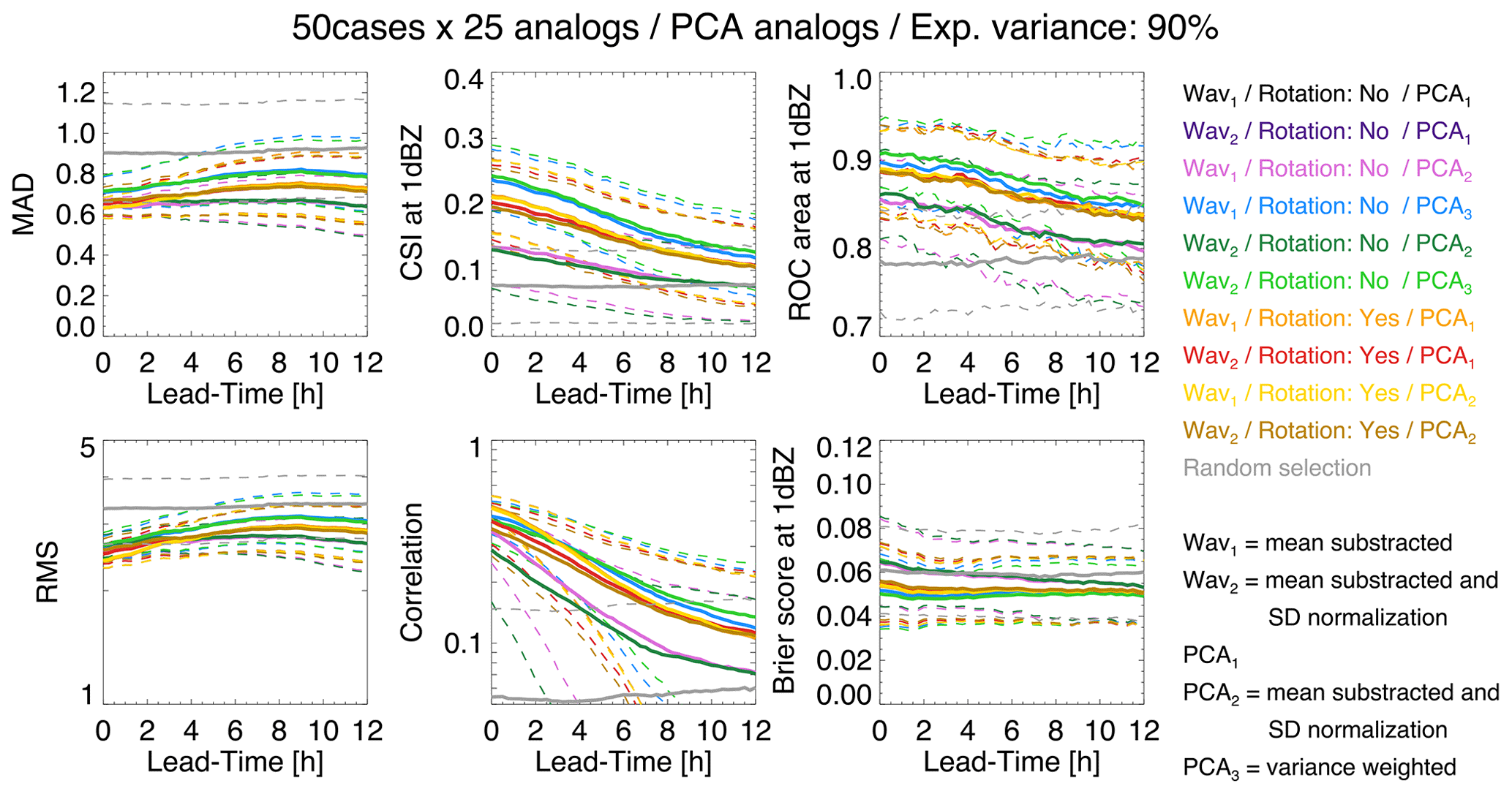
Figure 16Testing different PCA settings for retrieving analogues in the US. The dashed lines show the 25th and 75th percentile values of the score distribution.
According to MAD, RMSE and correlation, the best configuration is Wav1, Rotation (yes) and PCA2. Instead, according to CSI, ROC and Brier score, the best configurations are Wav2, Rotation (no) and PCA3 but also Wav1, Rotation (no) and PCA3. In summary, it seems that rotating eigenvectors degrades the categorical scores but improves the continuous scores, i.e. the ability to predict more intense precipitation. Weighting the PCs by the explained variance improves the categorical scores at the 1 dBZ threshold, i.e. the ability to separate wet and dry areas. It is not yet clear how these conclusions generalize to different climatic regions.
This analysis highlights that, once the attractor is defined, it is not that simple to retrieve analogue states. That is, practical implementation choices have an impact on the predictability estimations. Note that the low skill already at the start of the forecast (correlation ≈ 0.3–0.6 and CSI ≈ 0.15–0.25) is likely the result of verifying the forecast at the pixel resolution, while the retrieved analogues are only similar at large scales (see Sect. 2.2). Neighbourhood verification with the fraction skill score would give higher scores (Roberts and Lean, 2008).
Similar to Foresti et al. (2015), we also searched analogues by minimizing the Euclidean distance of the last two (instead of one) points in the PC space. Results were not surprising: the skill at the short lead times degraded and the one at the longer lead times improved, but only slightly.
This paper explored a framework to construct empirical low-dimensional precipitation attractors from multi-year archives of composite radar precipitation fields. The attractors were used to learn about the intrinsic predictability and various properties of precipitation fields. Data covering the Swiss Alps (2005–2010, 512×512 km2 domain) and the continental US (1996–2016, 4096×4096 km2 domain) were used.
We tested two approaches to defining the attractor. The first approach uses as phase space variables selected domain-scale statistics of precipitation fields that are relevant for nowcasting applications, for example the precipitation fraction, mean precipitation and slopes of the Fourier power spectrum, which characterize the spatial autocorrelation. The second approach derives the phase space in a more objective way by principal component analysis, which also considers the location of precipitation.
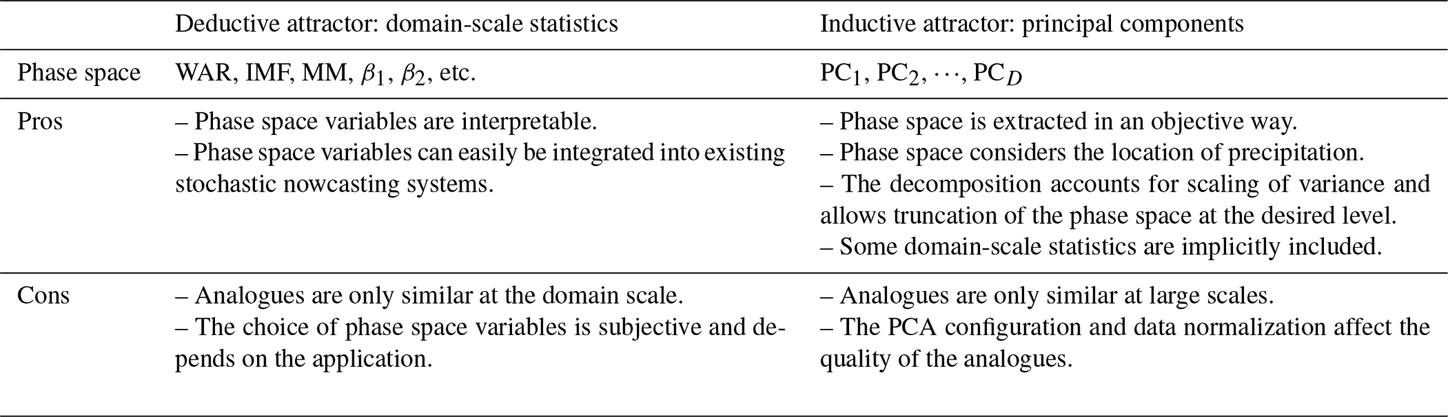
After defining the phase space variables, we studied the fractal properties and error growth from analogues within both attractors. The pros and cons of the two types of attractors are summarized in Table 2. The main conclusions are the following.
-
We could not find a unique objective way of defining the phase space of the attractor. That is, one is free to construct the attractor depending on the objective of the study or specific application.
-
Graphical representation of the attractor as the density of points in various combinations of phase space variables provides useful insight into data dependencies and precipitation regimes (e.g. stratiform vs. convective).
-
The magnitude of the scaling break in radially averaged power spectra of radar precipitation fields, previously observed by Gires et al. (2011) and Seed et al. (2013), is much more pronounced with isolated convective precipitation than stratiform precipitation.
-
Error growth from analogues retrieved by using domain-scale statistics starts slowly (0–1 h, reason mostly unknown), continues quickly (1–6 h, unpredictable convective precipitation growth and decay), and slows down again before predictability is lost to a large extent (6 h–20 d, more predictable synoptic scales).
-
The rate of error growth depends on the phase space used and the initial location within the attractor.
-
If the appropriate phase space variables are chosen, there is unexpectedly long intrinsic predictability of precipitation (several days), as shown with the US dataset.
-
Predictability of domain-scale statistics is longer in the US than CH, which is attributed mostly to the larger domain but also to the longer dataset.
-
By considering the spatial distribution of precipitation, PCA represents a useful framework for analysis, combination and simulation of precipitation fields.
-
Fourier analysis can be used to derive the spatial scales corresponding to eigenvector fields extracted by PCA.
-
The explained variance by PCA scales with both the ordinal PC number and corresponding spatial scale, which has a clear connection to Fourier-based decomposition of precipitation fields (e.g. Seed, 2003; Bowler et al., 2006).
-
Fractal analysis of the principal component time series reveals that low PCs have a stronger chaotic contribution than high PCs, which have a stronger stochastic component.
Table 2Advantages and disadvantages of the two types of attractors.
The application of tools used in chaos theory, such as time-delay embedding and the correlation dimension method, is complicated by the precipitation intermittency, finite event duration, non-Gaussian distribution and multifractal properties. These difficulties are also reflected in the analysis of derived phase space variables (MM, WAR, PCs, etc.). In addition, the validity of theorems and assumptions from chaos theory is pushed beyond their limits because precipitation is the result not only of dynamical processes, but also of (stochastic) microphysical processes. It is important to mention that the current study did not have the ambition to demonstrate that the precipitation attractor is of (finite) low dimensionality (see the discussion in Appendix D), but only to gain additional insight by testing different approaches.
Future perspectives comprise both improvements of the methodology and more practical applications. The methodology can be improved for example by exploring other phase space variables (e.g. orientation of anisotropy and precipitation translation speed), by using faster analogue retrieval methods (e.g. Franch et al., 2019), or by using more robust methods for estimating fractal dimensions (e.g. Golay and Kanevski, 2015; Camastra and Staiano, 2016; Pons et al., 2023). The size of the dataset could also be extended, although the main conclusions are not expected to change. The concept of an attractor could also have potential for automatic weather radar data quality control, where the interesting patterns are the outliers that deviate from the attractor.
Concerning possible applications, it is not yet clear how to exploit the gathered knowledge to improve precipitation forecasting in practice. For instance, both NWP forecasting and stochastic nowcasting methods are known to underestimate the forecast uncertainty. That is, the ensembles are under-dispersive. One possibility would be to drive stochastic simulations with the large-scale features given by analogues. Another possibility could be to seamlessly blend forecast probabilities derived from extrapolation nowcasts, NWP models and analogues.
Finally, a completely different methodology, which has attracted the attention of the atmospheric science community for quite some time, relies on the training of machine learning algorithms to optimally extract the localized predictable patterns from the data (Foresti et al., 2018, 2019). It could be insightful to use the methodology presented in this paper to understand what exactly was learned by machine learning algorithms in terms of predictability.
The discrete 2D power spectrum is defined as the squared norm of the complex Fourier transform:
where M is the number of image pixels, Z the precipitation field, the mean precipitation of the field, ℱ the fast Fourier transform operator, and (kx,ky) the wave numbers (corresponding to spatial frequencies). The 2D spectrum informs about the distribution of variance with spatial frequency and is a useful tool to analyse and model the spatial structure of rainfall fields (e.g. Seed, 2003; Nerini et al., 2017).
The spatial autocorrelation function (ACF) is obtained via the Wiener–Khinchin theorem as the inverse Fourier transform of the power spectrum under the assumption of stationarity (e.g. Nerini et al., 2017; Jameson et al., 2018):
where Var{Z} is the precipitation field variance. Since the autocorrelation and the spectrum form a Fourier transform pair, they both convey the same information, the former in physical space and the latter in the space of frequencies.
By assuming isotropy, from the 2D power spectrum we can derive a radially averaged 1D spectrum (RAPS):
where is the set of wave numbers for which . The same can be done for the 2D spatial autocorrelation.
Let XN,M be the archive of N radar images with M pixels. The PCA methodology consists of the following steps.
-
Set the value of pixels outside the radar domain to zero precipitation.
-
(Optionally) apply a logarithmic transformation to all precipitation values (use dBR or dBZ units; see Sect. 3.1).
-
Centre the data matrix XN,M by the column means, i.e. .
-
Compute the covariance matrix to estimate the linear dependence of variables, i.e. .
-
Diagonalize CM,M by eigenvalue decomposition (EVD), i.e. C=UVUT, where UM,M is the orthogonal matrix of eigenvectors (each column is one vector) and VM,M is the diagonal matrix of eigenvalues vi.
-
(Optionally) rotate the eigenvectors to enhance interpretation (e.g. Richman, 1986), e.g. using varimax.
-
Project the original data matrix into the space spanned by eigenvectors, i.e. .
Eigenvectors are sorted by decreasing amount of explained variance, which can be truncated such that D≪M.
An alternative way of performing PCA is by singular value decomposition (SVD) of the data matrix (e.g. Jolliffe, 2002). SVD factorization of the centred data matrix is obtained as
where L is the matrix of left singular vectors, R the matrix of right singular vectors, and S the diagonal matrix of singular values si. The eigenvalues can be calculated from the singular values as .
Since SVD does not require the computation of the covariance matrix, it has larger numerical stability than EVD. However, SVD is slower than EVD if N≫M. In such a case, one can perform a reduced SVD to avoid storing the large matrix LN,N. Finally, the projected data matrix is computed as .
For the Swiss archive, we used the SVD-based PCA decomposition available in the Python library sklearn (Pedregosa et al., 2011). For the US archive, we used the classical covariance-based PCA decomposition written in IDL.
An important concept for studying non-linear dynamical systems is the time-delay embedding theorem (Takens, 1981). Takens' theorem defines the conditions for which the dynamics of a smooth attractor can be reconstructed from a time series of observations of a single state space variable. Note that the assumption of smoothness may not apply beyond a certain data noise level (e.g. Schertzer et al., 2001).
Takens' theorem is applied by lagging multiple times the time series of a state space variable:
where xt is the original time series, xt−τ is the time series delayed by τ, and D is the dimensionality of the embedding space. In this paper, we have chosen τ to be equal to the first minimum of the temporal autocorrelation function.
The correlation dimension method, known as the Grassberger–Procaccia algorithm, estimates the fractal dimension of an attractor by counting the number of points that are contained in a D-dimensional sphere of increasing radius r, i.e. the correlation integral (Grassberger, 1986):
where H is the Heaviside function. The counting is performed for each point of the attractor. A log–log plot of C(r) vs. r gives an estimation of the fractal dimension:
where c is an offset and f is the fractal dimension (see Fig. D1 for an example using US data). In a 2D embedding space, randomly distributed points would give f≈2, while points along a straight line would give f≈1. In this paper, the terms fractal and correlation dimension are used interchangeably as measures of the intrinsic dimensionality of a dataset.
The Grassberger–Procaccia algorithm is known to underestimate the fractal dimension, which was the subject of controversial discussions questioning claims about the existence of low-dimensional attractors of atmospheric and hydrological processes (see e.g. Grassberger, 1986; Lorenz, 1991; Koutsoyiannis and Pachakis, 1996; Sivakumar et al., 2001a; Schertzer et al., 2001; Sivakumar et al., 2001b; Koutsoyiannis, 2006). As a consequence, new techniques are being developed to overcome its limitations (e.g. Golay and Kanevski, 2015; Camastra and Staiano, 2016).
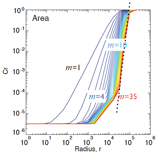
Figure D1Example estimation of the correlation dimension by finding the maximum slope in a log–log plot of the correlation integral C(r) vs. the search radius r. This example uses time-delay embedding on the time series of the radar precipitation area on the US domain.
Figures E1, E2 and E3 show various combinations of axis scaling and spread metrics that highlight the sensitivity of predictability estimations. Comments are in the respective captions.
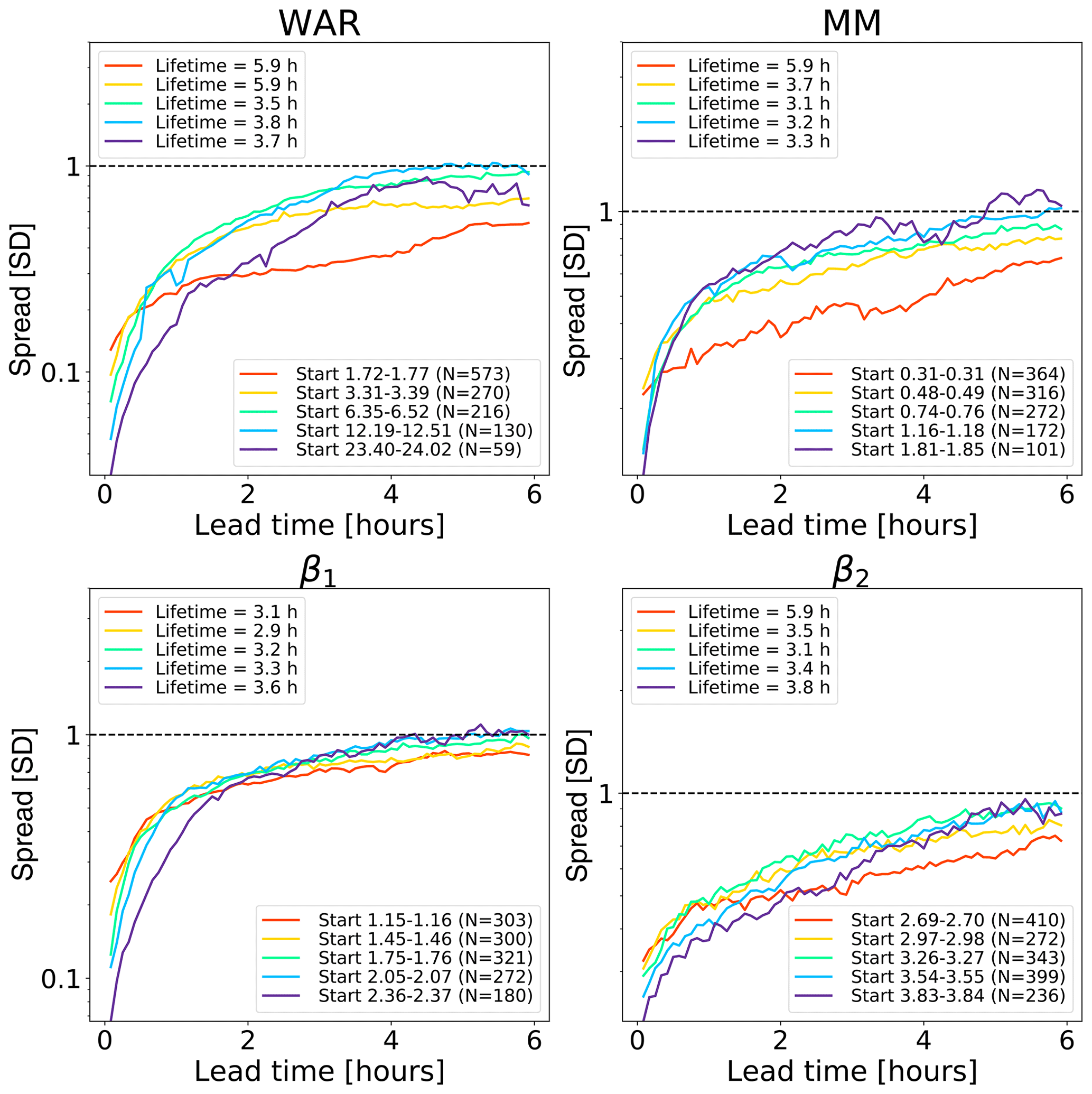
Figure E1Error growth of an ensemble of analogues starting from different initial conditions on the Swiss attractor. The x axis is linear, while the y axis is logarithmic, which is the standard way of analysing the initial error growth. The spread is computed according to Eq. (2). Most variables and initial conditions show a rapid growth of errors in the first 30–60 min. However, this initial growth is not linear enough to claim that error growth is exponential (in a linear time vs. linear error plot).
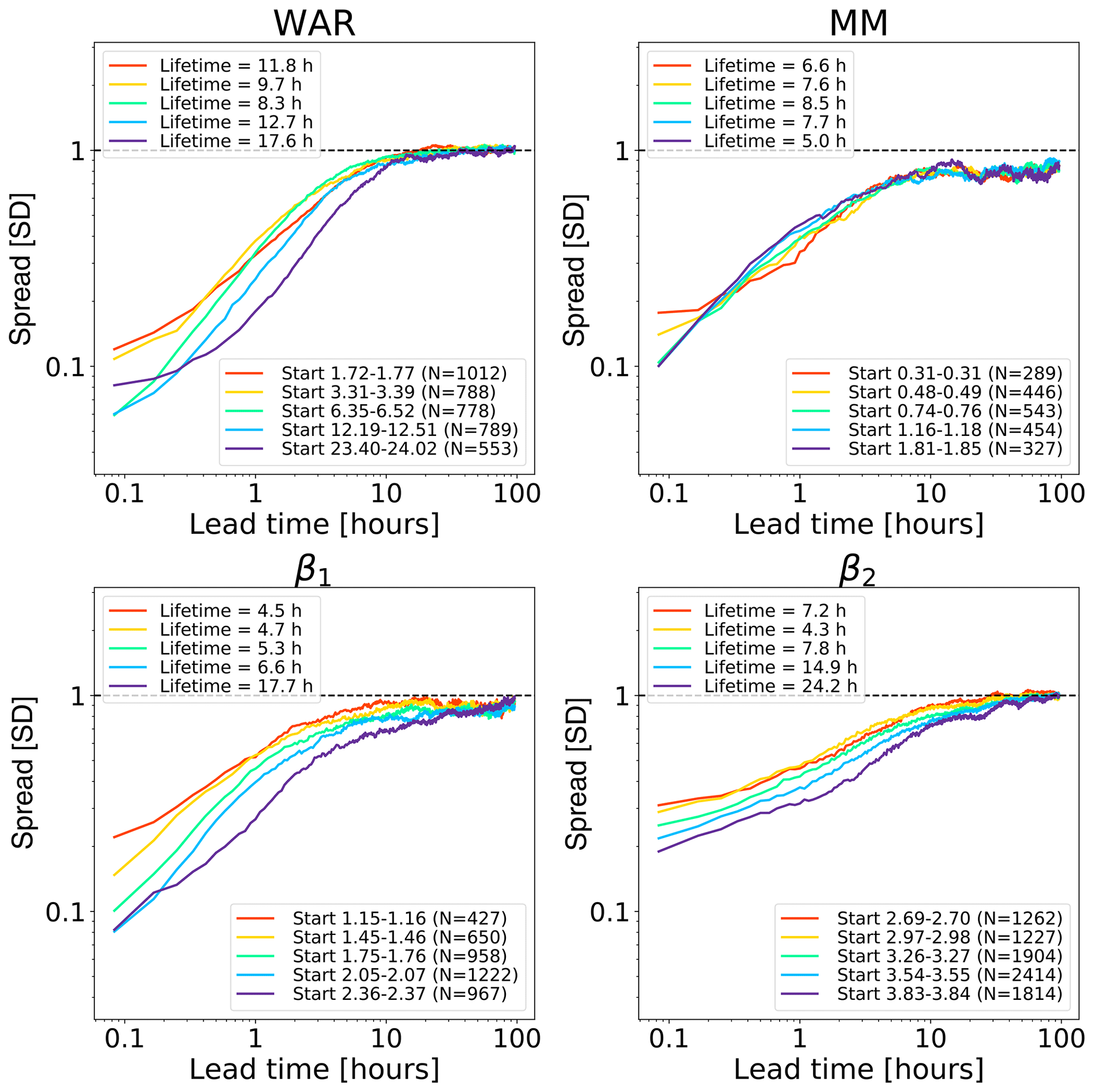
Figure E2Error growth of an ensemble of analogues starting from different initial conditions on the Swiss attractor. Both axes are logarithmic. The spread is computed according to Eq. (2). Compared to Fig. 9, the lifetime estimations are substantially shorter because the first derivatives of the kernel regression fit converge earlier (see Sect. 3.5).
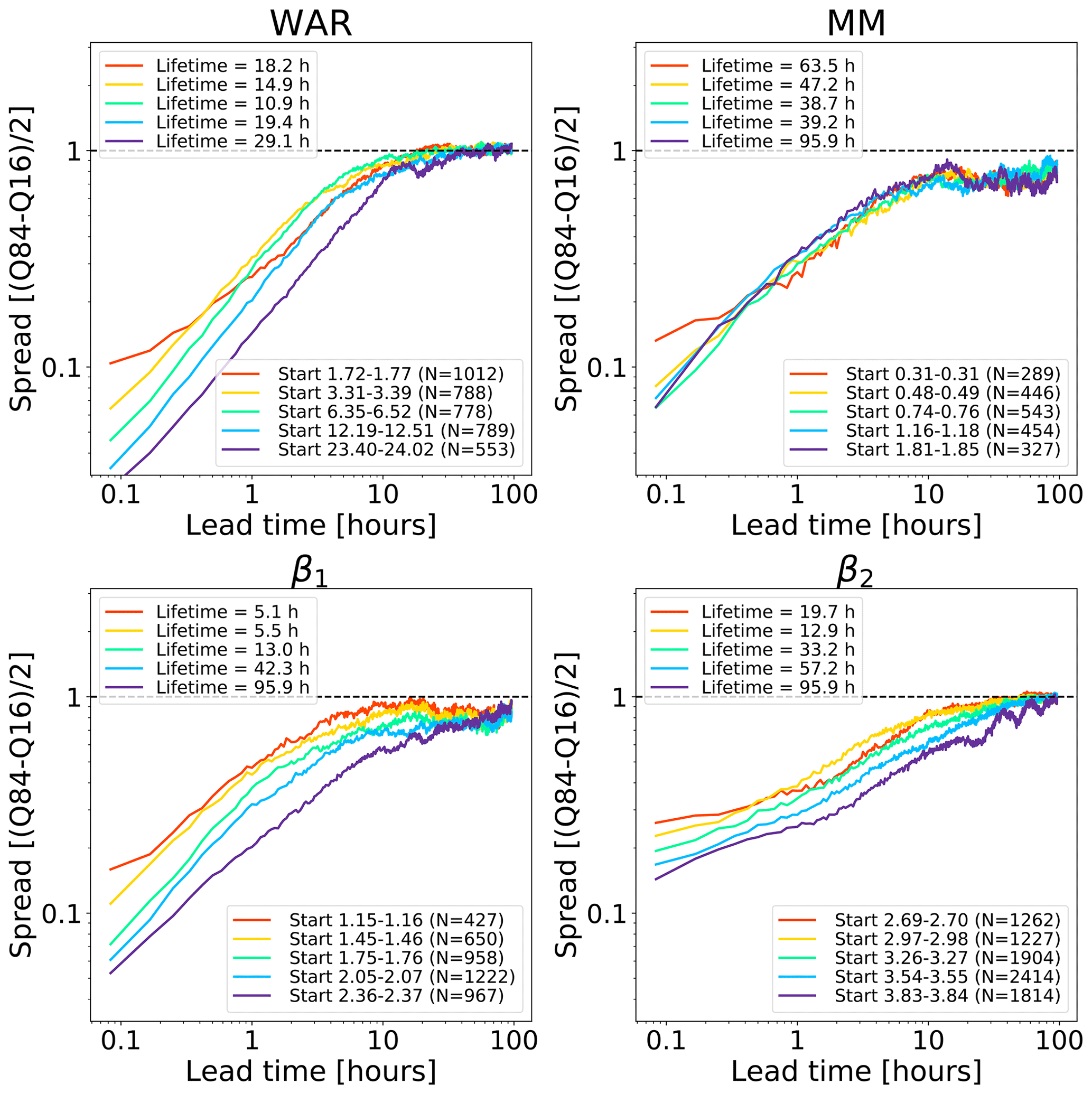
Figure E3Error growth of an ensemble of analogues starting from different initial conditions on the Swiss attractor. Both axes are logarithmic. The spread is computed according to Eq. (3). Compared to using the standard deviation (Fig. E2), the robust measure of spread gives straighter lines in the first 5–10 h, especially for the phase space variables WAR and β1.
Figure F1 shows the full coverage of the radar composite domain in the US.
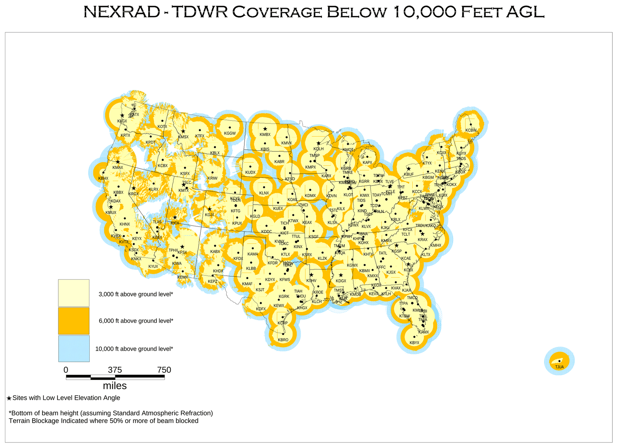
Figure F1Weather radar coverage in the continental US. Downloaded from https://www.roc.noaa.gov/WSR88D/Maps.aspx on 3 September 2023.
The code was developed in Python at MeteoSwiss and in IDL at McGill University and is not publicly available.
The US radar composite dataset compiled at McGill University is unfortunately not available. The Swiss composite radar dataset is also not currently available for free, but it will be made available in the future as part of the Open Government Data law. More information can be found here: https://github.com/MeteoSwiss/publication-opendata/ (Federal Office of Meteorology and Climatology MeteoSwiss and OGD@MeteoSwiss project team, 2024).
LF performed the analyses using the Swiss radar dataset and wrote the paper. BPT and AA performed the analyses using the US radar dataset. DN supported the implementation and interpretation of the results. MG, IS and UG supported the study with numerous discussions about radar precipitation, nowcasting and chaos theory. IZ originated the idea of the precipitation attractor and supervised the study with unparalleled enthusiasm and creativity for as long as he could.
The contact author has declared that none of the authors has any competing interests.
Publisher’s note: Copernicus Publications remains neutral with regard to jurisdictional claims made in the text, published maps, institutional affiliations, or any other geographical representation in this paper. While Copernicus Publications makes every effort to include appropriate place names, the final responsibility lies with the authors.
This study was supported by the Swiss National Science Foundation Ambizione project Precipitation attractor from radar and satellite data archives and implications for seamless very short-term forecasting (grant no. PZ00P2_161316). We are grateful to Alan Seed for the scientific discussions. Lea Beusch is thanked for reviewing an earlier version of the paper.
This research has been supported by the Swiss National Science Foundation SNSF (grant no. PZ00P2_161316).
This paper was edited by Stéphane Vannitsem and reviewed by two anonymous referees.
Abarbanel, H.: Analysis of Observed Chaotic Data, Springer, https://doi.org/10.1007/978-1-4612-0763-4, 1997. a, b
Alberti, T., Faranda, D., Lucarini, V., Donner, R. V., Dubrulle, B., and Daviaud, F.: Scale dependence of fractal dimension in deterministic and stochastic Lorenz-63 systems, Chaos, 33, 023144, https://doi.org/10.1063/5.0106053, 2023. a
Atencia, A. and Zawadzki, I.: A comparison of two techniques for generating nowcasting ensembles. Part I: Lagrangian ensemble technique, Mon. Weather Rev., 142, 4036–4052, 2014. a
Atencia, A. and Zawadzki, I.: A comparison of two techniques for generating nowcasting ensembles. Part II: Analogs selection and comparison of techniques, Mon. Weather Rev., 143, 2890–2908, 2015. a
Atencia, A. and Zawadzki, I.: Analogues on the Lorenz attractor and ensemble spread, Mon. Weather Rev., 145, 1381–1400, 2017. a, b
Atencia, A., Zawadzki, I., and Fabry, F.: Rainfall attractors and predictability, in: 36th Conference on Radar Meteorology, 16–20 September, Breckenridge, Colorado, https://ams.confex.com/ams/36Radar/webprogram/Paper228759.html (last access: 21 June 2024), 2013. a
Berenguer, M., Sempere-Torres, D., and Pegram, G. G.: SBMcast: An ensemble nowcasting technique to assess the uncertainty in rainfall forecasts by Lagrangian extrapolation, J. Hydrol., 404, 226–240, 2011. a
Bowler, N. E., Pierce, C. E., and Seed, A.: STEPS: A probabilistic precipitation forecasting scheme which merges an extrapolation nowcast with downscaled NWP, Q. J. Roy. Meteor. Soc., 132, 2127–2155, 2006. a, b, c
Camastra, F. and Staiano, A.: Intrinsic dimension estimation: Advances and open problems, Inform. Sci., 328, 26–41, 2016. a, b
De Cruz, L., Schubert, S., Demaeyer, J., Lucarini, V., and Vannitsem, S.: Exploring the Lyapunov instability properties of high-dimensional atmospheric and climate models, Nonlin. Processes Geophys., 25, 387–412, https://doi.org/10.5194/npg-25-387-2018, 2018. a
Fabry, F., Meunier, V., Treserras, B., Cournoyer, A., and Nelson, B.: On the climatological use of radar data mosaics: possibilities and challenges, B. Am. Meteorol. Soc., 98, 2135–2148, 2017. a
Federal Office of Meteorology and Climatology MeteoSwiss and OGD@MeteoSwiss project team: Open Government Data (OGD) provision, Github, https://github.com/MeteoSwiss/publication-opendata/, last access: 21 June 2024. a
Foresti, L., Panziera, L., Mandapaka, P. V., Germann, U., and Seed, A.: Retrieval of analogue radar images for ensemble nowcasting of orographic rainfall, Meteorol. Appl., 22, 141–155, 2015. a, b, c
Foresti, L., Sideris, I. V., Panziera, L., Nerini, D., and Germann, U.: A 10-year radar-based analysis of orographic precipitation growth and decay patterns over the Swiss Alpine region, Q. J. Roy. Meteor. Soc., 144, 2277–2301, https://doi.org/10.1002/qj.3364, 2018. a, b
Foresti, L., Sideris, I. V., Nerini, D., Beusch, L., and Germann, U.: Using a 10-year radar archive for nowcasting precipitation growth and decay – a probabilistic machine learning approach, Weather Forecast., 34, 1547–1569, https://doi.org/10.1175/WAF-D-18-0206.1, 2019. a
Franch, G., Jurman, G., Coviello, L., Pendesini, M., and Furlanello, C.: MASS-UMAP: Fast and Accurate Analog Ensemble Search in Weather Radar Archives, Remote Sens., 11, 2922, https://doi.org/10.3390/rs11242922, 2019. a
Germann, U., Galli, G., Boscacci, M., and Bolliger, M.: Radar precipitation measurement in a mountainous region, Q. J. Roy. Meteor. Soc., 132, 1669–1692, 2006a. a
Germann, U., Zawadzki, I., and Turner, B.: Predictability of Precipitation from Continental Radar Images. Part IV: Limits to Prediction, J. Atmos. Sci., 63, 2092–2108, https://doi.org/10.1175/JAS3735.1, 2006b. a, b, c
Germann, U., Boscacci, M., Clementi, L., Gabella, M., Hering, A., Sartori, M., Sideris, I. V., and Calpini, B.: Weather Radar in Complex Orography, Remote Sens., 14, 503, https://doi.org/10.3390/rs14030503, 2022. a
Gires, A., Tchiguirinskaia, I., Schertzer, D., and Lovejoy, S.: Multifractal and spatio-temporal analysis of the rainfall output of the Meso-NH model and radar data, Hydrolog. Sci. J., 56, 380–396, https://doi.org/10.1080/02626667.2011.564174, 2011. a, b, c
Golay, J. and Kanevski, M.: A new estimator of intrinsic dimension based on the multipoint Morisita index, Pattern Recogn., 48, 4070–4081, 2015. a, b
Grassberger, P.: Do climatic attractors exist?, Letters to Nature, 323, 609–611, 1986. a, b
Grassberger, P. and Procaccia, I.: Measuring the strangeness of strange attractors, Phys. D, 9, 189–208, 1983. a
Houze, R.: Cloud Dynamics, Academic Press, ISBN 9780123742667, 2014. a
Jameson, A., Larsen, M., and Kostinski, A.: On the Detection of Statistical Heterogeneity in Rain Measurements, J. Atmos. Ocean. Tech., 35, 1399–1413, 2018. a
Jolliffe, I.: Principal Component Analysis, 2nd Edn., Springer, https://doi.org/10.1007/978-1-4757-1904-8, 2002. a, b
Kantz, H. and Schreiber, T.: Nonlinear Time Series Analysis, 2nd Edn., Cambridge University Press, https://doi.org/10.1017/CBO9780511755798, 2004. a, b
Koutsoyiannis, D.: On the quest of chaotic attractors in hydrological processes, Hydrolog. Sci., 51, 1065–1091, 2006. a
Koutsoyiannis, D. and Pachakis, D.: Deterministic chaos versus stochasticity in analysis and modeling of point rainfall series, J. Geophys. Res.-Atmos., 101, 26441–26451, 1996. a
Li, J. and Ding, R.: Temporal-spatial distribution of atmospheric predictability limit by local dynamical analogues, Mon. Weather Rev., 139, 3265–3283, 2011. a
Lichtenberg, A. J. and Lieberman, M. A.: Regular and Chaotic Dynamics, no. 38 in Applied Mathematical Sciences, Springer-Verlag, New York, NY, 2nd Edn., https://doi.org/10.1007/978-1-4757-2184-3, 1992. a, b
Link, R., Snyder, A., Lynch, C., Hartin, C., Kravitz, B., and Bond-Lamberty, B.: Fldgen v1.0: an emulator with internal variability and space–time correlation for Earth system models, Geosci. Model Dev., 12, 1477–1489, https://doi.org/10.5194/gmd-12-1477-2019, 2019. a
Lorenz, E. N.: Empirical orthogonal functions and statistical weather prediction, Tech. Rep. Scientific Report No. 1, Statistical Forecasting Project, Air Force Research Laboratories, Office of Aerospace Research, USAF, Bedford, MA, 1956. a, b
Lorenz, E. N.: Deterministic nonperiodic flow, J. Atmos. Sci., 20, 130–141, 1963. a, b, c
Lorenz, E. N.: Atmospheric predictability as revealed by naturally occurring analogues, J. Atmos. Sci., 26, 636–646, 1969. a, b
Lorenz, E. N.: Dimensions of weather and climate attractors, Letters to Nature, 353, 241–244, 1991. a
Lorenz, E. N.: Predictability – a problem partly solved, in: Proc. Seminar on Predictability, Volume 1. European Centre for Medium-Range Weather Forecast, Shinfield Park, Reading, Berkshire, United Kingdom, https://doi.org/10.1017/CBO9780511617652.004, 1996. a, b
Lovejoy, S. and Schertzer, D.: The Weather and Climate: Emergent Laws and Multifractal Cascades, Cambridge University Press, https://doi.org/10.1017/CBO9781139093811, 2013. a, b, c
Menabde, M.: Bounded lognormal cascades as quasi-multiaffine random processes, Nonlin. Processes Geophys., 5, 63–68, https://doi.org/10.5194/npg-5-63-1998, 1998. a
Nerini, D., Besic, N., Sideris, I., Germann, U., and Foresti, L.: A non-stationary stochastic ensemble generator for radar rainfall fields based on the short-space Fourier transform, Hydrol. Earth Syst. Sci., 21, 2777–2797, https://doi.org/10.5194/hess-21-2777-2017, 2017. a, b, c, d, e, f
Nerini, D., Foresti, L., Leuenberger, D., Robert, S., and Germann, U.: A reduced-space ensemble Kalman filter approach for flow-dependent integration of radar extrapolation nowcasts and NWP precipitation ensembles, Mon. Weather Rev., 147, 987–1006, https://doi.org/10.1175/MWR-D-18-0258.1, 2019. a, b
Nicolis, C., Vannitsem, S., and Royer, J.-F.: Short-range predictability of the atmosphere: Mechanisms for superexponential error growth, Q. Roy. Meteor. Soc., 121, 705–722, 1995. a
Palmer, T. and Hagedorn, R. (Eds.): Predictability of Weather and Climate, Cambridge University Press, https://doi.org/10.1017/CBO9780511617652, 2006. a
Pedregosa, F., Varoquaux, G., Gramfort, A., Michel, V., Thirion, B., Grisel, O., Blondel, M., Prettenhofer, P., Weiss, R., Dubourg, V., Vanderplas, J., Passos, A., Cournapeau, D., Brucher, M., Perrot, M., and Duchesnay, E.: Scikit-learn: Machine Learning in Python, J. Mach. Learn. Res., 12, 2825–2830, 2011. a
Pegram, G. G. S. and Clothier, A. N.: High resolution space-time modelling of rainfall: The “String of Beads” model, J. Hydrol., 241, 26–41, 2001. a, b, c, d
Pons, F., Messori, G., and Faranda, D.: Statistical performance of local attractor dimension estimators in non-Axiom A dynamical systems, Chaos, 33, 073143, https://doi.org/10.1063/5.0152370, 2023. a
Pulkkinen, S., Nerini, D., Pérez Hortal, A. A., Velasco-Forero, C., Seed, A., Germann, U., and Foresti, L.: Pysteps: an open-source Python library for probabilistic precipitation nowcasting (v1.0), Geosci. Model Dev., 12, 4185–4219, https://doi.org/10.5194/gmd-12-4185-2019, 2019. a
Richman, M. B.: Review article: Rotation of principal components, J. Climatol., 6, 293–335, 1986. a, b, c, d, e
Roberts, N. M. and Lean, H. W.: Scale-Selective Verification of Rainfall Accumulations from High-Resolution Forecasts of Convective Events, Mon. Weather Rev., 136, 78–97, https://doi.org/10.1175/2007MWR2123.1, 2008. a
Schertzer, D. and Lovejoy, S.: Physical modeling and analysis of rain and clouds by anisotropic scaling multiplicative processes, J. Geophys. Res., 92, 9693–9714, 1987. a, b
Schertzer, D., Tchiguirinskaia, I., Lovejoy, S., Hubert, P., Bendjoudi, H., and Larchevêque, M.: Which chaos in the rainfall–runoff process? Disussion of “Evidence of chaos in the rainfall-runoff process”, Hydrolog. Sci. J., 47, 139–148, 2001. a, b, c
Schiemann, R., Liniger, M., and Frei, C.: Reduced space optimal interpolation of daily rain gauge precipitation in Switzerland, J. Geophys. Res., 115, D14109, https://doi.org/10.1029/2009JD013047, 2010. a
Seed, A.: A dynamic and spatial scaling approach to advection forecasting, J. Appl. Meteorol., 42, 381–388, 2003. a, b, c, d, e
Seed, A., Pierce, C. E., and Norman, K.: Formulation and evaluation of a scale decomposition-based stochastic precipitation nowcast scheme, Water Resour. Res., 49, 6624–6641, 2013. a, b, c, d, e, f
Sideris, I.: Measure of orbital stickiness and chaos strength, Phys. Rev. E, 73, 066217, https://doi.org/10.1103/PhysRevE.73.066217, 2006. a
Sideris, I. V., Foresti, L., Nerini, D., and Germann, U.: NowPrecip: localized precipitation nowcasting in the complex terrain of Switzerland, Q. J. Roy. Meteor. Soc., 146, 1768–1800, https://doi.org/10.1002/qj.3766, 2020. a, b, c
Simoncelli, E. and Olshausen, B.: Natural image statistics and neural representation, Annu. Rev. Neurosci., 4, 1193–2216, 2001. a
Sivakumar, B., Berndtsson, R., Olsson, J., and Jinno, K.: Reply to “Which chaos in the rainfall-runoff process”, Hydrolog. Sci. J., 47, 149–158, 2001a. a
Sivakumar, B., Berndtsson, R., Olsson, J., and Jinno, K.: Evidence of chaos in the rainfall-runoff process, Hydrolog. Sci. J., 46, 131–145, 2001b. a
Surcel, M., Zawadzki, I., and Yau, M. K.: A study on the scale dependence of the predictability of precipitation patterns, J. Atmos. Sci., 72, 216–235, 2015. a
Takens, F.: Detecting strange attractors in turbulence, in: Dynamical Systems and Turbulence, Lecture Notes in Mathematics, Springer, vol. 898, 366–381, ISBN 978-3-540-38945-3, 1981. a, b
Toth, Z.: Estimation of atmospheric predictability by circulation analogues, Mon. Weather Rev., 119, 65–72, 1991. a
Van Den Dool, H. M.: Searching for analogs: how long must we wait?, Tellus A, 46, 314–324, 1994. a, b
Villarini, G. and Krajewski, W.: Review of the Different Sources of Uncertainty in Single Polarization Radar-Based Estimates of Rainfall, Surv. Geophys., 31, 107–129, https://doi.org/10.1007/s10712-009-9079-x, 2010. a
- Abstract
- Introduction
- Data and conceptual framework
- Precipitation attractors based on domain-scale statistics
- Precipitation attractors based on principal component analysis
- Conclusions
- Appendix A: Fourier analysis of precipitation fields
- Appendix B: Principal component analysis
- Appendix C: Time-delay embedding
- Appendix D: Correlation dimension method
- Appendix E: Axis-scaling effect on error growth
- Appendix F: CONUS coverage
- Code availability
- Data availability
- Author contributions
- Competing interests
- Disclaimer
- Acknowledgements
- Financial support
- Review statement
- References