the Creative Commons Attribution 4.0 License.
the Creative Commons Attribution 4.0 License.
 | 17 Jan 2024
Aggregation of slightly buoyant microplastics in 3D vortex flows
Lawrence J. Pratt
Michael Dotzel
Although the movement and aggregation of microplastics at the ocean surface have been well studied, less is known about the subsurface. Within the Maxey–Riley framework governing the movement of small, rigid spheres with high drag in fluid, the aggregation of buoyant particles is encouraged in vorticity-dominated regions. We explore this process in an idealized model that is qualitatively reminiscent of a 3D eddy with an azimuthal and overturning circulation. In the axially symmetric state, buoyant spherical particles that do not accumulate at the top boundary are attracted to a loop consisting of periodic orbits. Such a loop exists when drag on the particle is sufficiently strong. For small, slightly buoyant particles, this loop is located close to the periodic fluid parcel trajectory. If the symmetric flow is perturbed by a symmetry-breaking disturbance, additional attractors for small, rigid, slightly buoyant particles may arise near periodic orbits of fluid parcels within the resonance zones created by the disturbance. Disturbances with periodic or quasiperiodic time dependence may produce even more attractors, with a shape and location that recurs periodically. However, not all such loops attract, and rigid particles released in the vicinity of one loop may instead be attracted to a nearby attractor. Examples are presented along with mappings of the respective basins of attraction.
- Article
(6442 KB) - Full-text XML
-
Supplement
(531 KB) - BibTeX
- EndNote


Marine microplastic pollution has been a rising concern for the ocean environmental and for human health. Microplastics (scales <5 mm) and nanoplastics (scales <1 µm) have been found in the tissues of marine animals, some of which are consumed by humans (Landrigan et al., 2023). This comes at a time when the global production of plastics is projected to increase. Observations of marine microplastics have conventionally been carried out using net tows and have mostly occurred at or near the sea surface (van Sebille et al., 2015). However, the density of many types of microplastic particles, including high-density polyethylene, is sufficiently close to that of seawater that suspension within the water column for long periods of time is feasible. For the near-surface microplastics, Kukulka et al. (2012) and Kooi et al. (2016) present observational evidence for the fast decay in concentrations with depth over the top 5–20 m of the water column, with the vertical penetration of plastic particles dependent on the wind speed. Pabortsava and Lampitt (2020), on the other hand, show observational evidence for much deeper, sub-mixed-layer subsurface peaks for three common types of microplastics in the Atlantic Ocean. Processes such as biofouling and biogeochemical degradation or photodegradation might increase the density of the plastic particles and eventually lead to the sinking of microplastics from the surface into the deeper part of the water column (Kaiser et al., 2017; Kreczak et al., 2021; Kvale et al., 2020). Consumption by biomass with the subsequent downward vertical transport is another vehicle for redistributing microplastics from the surface down. For example, Choy et al. (2019) suggest that this mechanism, specifically consumption by pelagic red crabs and giant larvaceans, was responsible for the subsurface peaks in plastic particles concentrations observed at depths near 250 m in Monterey Bay. Thus, microplastics have been found well beneath the ocean surface, but less is known regarding their spatiotemporal and size/density distributions (Shamskhany et al., 2021).
A potentially important aspect of the movement of plastics and microplastics is aggregation, a process that occurs at the surface over large scales near the centers of the five major subtropical gyres and has been attributed to Ekman drift, windage, and inertia (Beron-Vera, 2021). Many early models concentrated on the ocean surface, but Wichmann et al. (2019) highlighted the importance of resolving the full 3D circulation. If aggregation also occurs below the surface, well beneath the direct influence of Ekman layers, the dynamics is likely to be different. Indeed, modeling results by Wichmann et al. (2019), based on a framework created by Lange and van Sebille (2017) and Delandmeter and van Sebille (2019), suggest that the large-scale accumulation associated with the garbage patches disappears below 60 m depth.
To avoid confusion, we will refer to infinitesimal fluid elements as “fluid parcels” and to rigid plastic particles of finite size as “rigid particles”. Typically, the position xp(t) of a rigid particle is tracked according to the following:
where u is the fluid velocity and dxb is an extra displacement due to the non-fluid nature of the rigid particle. The user can introduce custom schemes for calculating contributions to dxb due to factors such as windage and inertia (e.g., Beron-Vera et al., 2016), turbulent diffusion (e.g., Kukulka et al., 2012), and wave-induced Stokes drift (Onink et al., 2019). Eulerian schemes in which plastic particles are treated as concentrations are rare, but Mountford and Morales Maqueda (2019) developed an Eulerian model in which concentrations are advected by the fluid and are subject to parameterized turbulence as well as sinking or rising according to a simple law involving buoyancy and friction. In a similar fashion, Kvale et al. (2020) proposed an Eulerian model for the biological uptake and the resulting redistribution of microplastics.
An alternative approach would be to use the Maxey–Riley equation (discussed below) to solve for the rigid-particle velocity, v, and then use the latter to compute the trajectory of that rigid particle, i.e., . This equation would account for the non-fluid-following effects in a deductive way; however, the resulting sixth-order system (for the three components of velocity and position) would be computationally challenging. To better understand the implications of this approach while avoiding the computational burden and complexity, we will analyze the movement and aggregation of rigid particles using a Maxey–Riley framework in connection with an idealized, analytically prescribed, 3D vortex flow that qualitatively resembles the geometry of the circulation in an ocean eddy but is not a solution to any dynamical oceanographic equations of motion. As shown by Pratt et al. (2014) and Rypina et al. (2015), kinematic models that reproduce the correct geometry are able to also reproduce the important Lagrangian features of the flow. Even in our simple flow, aggregation is nontrivial, often with multiple attractors present and lack of attraction in some circumstances. Thus, we wanted to thoroughly explore this simple example before investigating more realistic oceanic flows. We note that other idealized studies have been carried out in connection with 2D wave fields and vortex flows (e.g., DiBenedetto et al., 2018; DiBenedetto and Ouellette, 2018; Kelly et al., 2021).
Aggregation can be attributed to the presence of an attractor: here, an object with a dimension less than 3 that is set up by the fluid circulation patterns and towards which rigid-particle trajectories attract. As long as the fluid is incompressible, fluid parcels will not experience attraction and will not aggregate, but plastic particles may do so. Note also that, because each attractor is generally associated with its corresponding basin of attraction, if rigid particles are introduced outside of the basin of attraction, they will not be attracted and will not aggregate towards this attractor.
In order to reach a better understanding of what leads to attraction and attractors in 3D flows, we explore a simple canonical example in geophysical fluid dynamics, namely the flow in a rotating cylinder. This flow resembles some of the characteristics of ocean eddies, including a horizontal swirl and an overturning component in the vertical, but is much less complex than any realistic oceanic eddy. Specifically, we use a simple analytically prescribed phenomenological velocity introduced by Rypina et al. (2015). The Lagrangian properties of this circulation have been previously studied (Fountain et al., 2000; Pratt et al., 2014; Rypina et al., 2015), allowing us to begin to investigate inertial rigid particles from an established base of knowledge. A prior theory (Haller and Sapsis, 2008) governing the movement of rigid particles with high drag indicates that accumulation is favored for slightly buoyant particles in flows dominated by vorticity, and this also motivates our choice of background flow. Identification of the attractors that can arise in this flow field, evaluating their reach and domains of attraction, and clarifying the circumstances that lead to their formation are the primary objectives of this work. Although motivated by the problem of marine microplastics, this study is, for now, mainly a curiosity-driven research that aims to develop a basic understanding of the mechanisms that might lead to aggregation of rigid particles in 3D flows. The hope is that, with such basic understanding in hand, one could later start investigating aggregation phenomena in more complex and more realistic ocean mesoscale and submesoscale eddying flows.
The physics of the motion of a small, rigid sphere that moves with velocity v(t) through a fluid with pre-existing velocity distribution u(x,t) has been the subject of investigation by Stokes (1851), Basset (1988), Boussinesq (1903), Faxén (1922), Oseen (1927), Tchen (1947), and many others, and it was put in a unifying framework by Maxey and Riley (1983). More recent theoretical extensions include Beron-Vera et al. (2019) and Beron-Vera (2021). We will use a form of the Maxey–Riley equation that has been extended to include constant frame rotation with angular velocity Ω∗:
The frame rotation was introduced into the nonrotating Maxey–Riley equation by replacing
where subscript “s” denotes stationary frame and subscript “r” represents rotating frame. Alternatively, transformation into a rotating frame can be done following the variational method of Ripa (1987). The subscripts “r” are then dropped in Eq. (1) and all subsequent equations, as all variables are in the rotating frame. For nonspherical, rigid particles, adjustments to the coefficients within the Maxey–Riley equations can be made to account for elliptical shapes (see, e.g., DiBenedetto et al., 2018; DiBenedetto and Ouellette, 2018, and references therein) but at the cost of adding a third vector equation for the orientation of the ellipsoid. However, real microplastics often have complex tangled-filament-like shapes which are poorly represented by an ellipsoid, and no corrections for tangled filaments are currently available.
In Eq. (1), which is a statement of Newton's second law for the rigid particle, the right-hand side represents (in order) the effects of inertia, added mass, drag, buoyancy, the Coriolis acceleration associated with the added mass, the Coriolis acceleration associated with the fluid motion, the Coriolis acceleration associated with the particle mass, and centrifugal acceleration. A similar equation has previously been derived by Beron-Vera et al. (2019), although the centrifugal acceleration does not appear there explicitly, having been combined with the acceleration due to gravity in order to define an effective gravity and corresponding geopotential. Coordinates are then imagined to be aligned with geopotential surfaces, although standard spherical or Cartesian coordinates are usually used in practice (Vallis, 2006). Our explicit retention of the centrifugal acceleration will later allow absolute vorticity to arise naturally as a quantity of central importance. We have omitted the lift force, the Basset history force, and the Faxén corrections (Gatignol, 1983). Faxén corrections account for the variation in the flow across the rigid particle and are proportional to a2Δu. For a particle size that is much smaller than the typical length scale of the flow, these corrections are small and typically neglected (Haller and Sapsis, 2008; Beron-Vera et al., 2019). The history term, which is an integral along a particle path, accounts for the boundary layer effects that a particle leaves behind. It is typically ignored under the assumption that the chances of other particles crossing that localized boundary layer before it decays are small (Beron-Vera et al., 2019; see also Langlois et al., 2015; Daitche and Tél, 2011, for more info on the influence of the history term on the behavior of rigid particles). Finally, the lift force arises when a particle rotates in a horizontally sheared flow. As shown in Beron-Vera et al. (2019), the inclusion of the lift force leads to the next-order correction in the slow-manifold approximation and, thus, can also be neglected for small . In Eq. (1), ρp and ρf are densities of the rigid particle and the fluid, respectively; d is the particle radius; ν is viscosity of the fluid; g is the gravity vector; and is the fluid material derivative, evaluated for undisturbed fluid velocity at the position of the center of the rigid particle. The position x(t) of a particle is determined by
and together Eqs. (1) and (2) compose a coupled, sixth-order system for the computation of the particle position and velocity as functions of time.
If the velocities and lengths are nondimensionalized using characteristic scales U and L for the background fluid flow and is used as a timescale, then Eq. (2) remains formally unchanged while the nondimensional form of Eq. (1) is as follows:
where ; ; ; and is the Stokes number, the ratio of the adjustment timescale of a particle (due to drag) to the timescale of the background flow. For , viscous drag is the dominant force acting on the particle, implying that a particle with an initial velocity differing by an amount from the local fluid velocity will be rapidly accelerated over a timescale to a velocity proximal to that of the fluid. Thereafter, the particle will undergo a slow evolution in which the weaker forces due to inertia, added mass, and buoyancy cause slight departures from the movement of the fluid itself.
The limit constitutes a singular perturbation of Eq. (3), a problem that can be addressed using an approach due to Fenichel (1979) that was originally formally developed for a steady background flow but that has been extended by Haller and Sapsis (2008) to include a time-varying background flow. In either case, it can be shown that, following the initial viscous adjustment, the particle position and velocity tend toward a subspace or “slow manifold” on which the particle velocity is determined directly by the fluid velocity through an “inertial” equation, here extended to include frame rotation:
This result is the same as that obtained by Beron-Vera et al. (2019), provided that their gravity vector is interpreted as our gr. The same authors also present more general cases, including those with the lift force and on the sphere. In the Supplement, we present a simple derivation of Eq. (4) based on a multiscale expansion. It provides a quick, although less rigorous, alternative to the Fenichel approach.
A chief advantage of the slow-manifold reduction is that the sixth-order system given by Eqs. (2) and (3), in which particle velocity needs to be solved for, is reduced to a third-order system given by Eqs. (2) and (4), where the particle velocity is explicitly written as a function of fluid velocity and flow and particle parameters (and thus is known). The bracketed expression in Eq. (4), which determines the velocity of the rigid particle relative to the fluid, is nothing more than , where τij is the stress tensor for the fluid. Thus, the relative velocity of a rigid particle on the slow manifold is in the same direction as the net force that would act on a fluid parcel occupying the same space. Ordinarily, for a fluid parcel, that force would equate to an acceleration; however, on the slow timescale, the relative particle velocity points in the same direction as the net fluid force and its magnitude is proportional to . As the aggregation of rigid particles requires departures of the particle velocity from the (divergence-free) velocity field of the fluid, one can expect that aggregation will occur more slowly if d and are small or if ν is large. At the same time, the existence of attractors internal to the fluid may depend on being small. For example, a large density difference may mean that rigid particles simply sink to the bottom or rise to the surface (and are thus attracted to attractors external to the fluid interior).
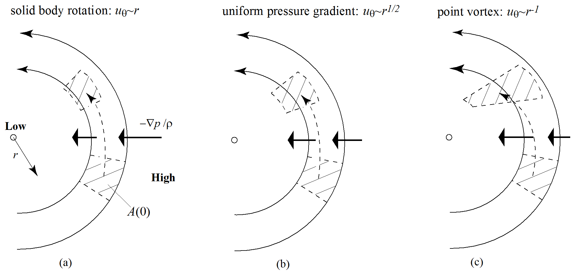
Figure 1Three types of 2D eddies with zero frame rotation and for which gravity is imagined to be zero: solid-body rotation (a), constant pressure gradient (b), and point vortex (c). In each case, the crosshatched area represents a concentration of rigid particles with area A(t).
As pointed out by Haller and Sapsis (2008) (see also Beron-Vera et al., 2019), we can consider a continuous concentration of rigid particles with similar properties and with smoothly varying velocity given by Eq. (4). The aggregation of such a concentration would appear to require that the divergence of that velocity be negative (although an apparent counterexample is given in Fig. 1c, presented later). Following Haller and Sapsis (2008), consider the evolution of a material volume of rigid particles. The time rate of change in this volume is
where for an incompressible fluid. Shrinking V to an infinitesimal size allows the right-hand side to be approximated by V times the local value in the integrand, and the result may be integrated in time, yielding the following:
Here, is the 3D Okubo–Weiss parameter (Okubo, 1970; Weiss, 1991), where ζr represents the relative vorticity vector for the fluid, is the strain tensor, and |S| is its Frobenius norm. The final step in Eq. (6) follows from introduction of the absolute vorticity vector
and the corresponding function . This result could have been anticipated from the fact that the vorticity and the absolute vorticity are the same in the rest frame.
We note that for a volume V of any size,
Here, nj denotes the components of the outward unit vector normal to the bounding surface AV. The first equality in Eq. (8) is a modest modification of Eq. (31) from Haller and Sapsis (2008), and, as mentioned above, one could probably have guessed that our more general result could be obtained by replacing Q with Qa. The remainder of the equation expresses volume changes in terms of the fluid stresses. Thus, for buoyant particles, a volume V(t) of any size will contract if the force normal to AV due to the fluid stresses, integrated around AV, is inward. In many cases, including quasigeostrophic eddies and gyres, internal waves, and the surface gravity waves considered by DiBenedetto et al. (2018) and DiBenedetto and Ouellette (2018) and all inviscid flows, the stress tensor is dominated by pressure, i.e., , so the tendency to aggregate is determined entirely by the pressure field.
In general, Qa can change sign along a particle trajectory, making it hard to predict whether the surrounding volume shrinks or expands with time. If a buoyant particle is trapped in a region in which Qa is predominately positive, then this region is a good candidate for aggregation. Persistent ocean eddies and other vortical structures are possibilities, not only because vorticity tends to dominate over strain there but also because such features have the ability to trap fluid for long periods of time. For dense particles, contraction occurs in areas dominated by strain, and it has been shown that aggregation of heavy particles can occur in strain-dominated filaments that arise in particle-laden turbulent flows, although the considered particle-to-fluid density differences tend to be quite large (see Brandt and Coletti, 2022, for a review). In our study, we will focus on vortex flows reminiscent of ocean eddies and on lower-dimensional objects within such flows that can act as attractors for buoyant particles.
A simple example of aggregation is given by Haller and Sapsis (2008), who argue that the elliptical center of a steady, non-divergent 2D eddy, with 0, acts as an attractor for buoyant particles. Here, Qa (now =Qr) is ostensibly positive near the elliptical center of the eddy, corresponding to contraction of the phase space (which, in our case, coincides with the physical space) of the rigid-particle motion. As the central fixed point of the velocity field of the eddy is also a fixed point of the slow-manifold particle velocity (Eq. 4), buoyant particles initiated about the center should migrate towards the center. If the eddy is inviscid and its streamlines are circular, then the pressure and azimuthal velocity are related by the cyclostrophic balance , so that 2, and for an eddy in solid-body rotation ( 2. As suggested in Fig. 1a, a small concentration of rigid particles indicated by the crosshatched area shrinks as it moves towards the center of the eddy. The contraction is partially due to the geometric effect of movement towards smaller radius (term but also due to the fact that the pressure gradient decreases to zero as the center is approached and, thus, the inner edge of the path moves more slowly inward than the outer part (term ). In the case of solid-body rotation, the two terms contribute equally. A second example (Fig. 1b) is of an eddy with an azimuthal velocity given by . Here, and 2, so the contraction of the patch is entirely due to the geometric effect of its movement towards a smaller radius. The most curious case is that of a point vortex: , for which 2. Here, the vorticity is zero away from the eddy center and the velocity field is dominated by strain. The pressure gradient increases as the center of the vortex is approached, meaning that the inner part of the patch moves towards the center more rapidly than the outer portion (Fig. 1c) and this tendency (quantified by the factor ) surpasses the tendency towards geometrical contraction (quantified by the factor ). Thus, the area of the patch expands as rigid particles are drawn towards the center of the vortex. Note, however, that a patch surrounding the center of the vortex can only shrink. This behavior is made possible by the singularity at the center, and, although this feature is artificial, point vortices are often used in idealized models of fluid flow and will act as sinks or “black holes” for buoyant particles even though 2Qr<0.
The sign of Qa is clearly not the whole story and does not encompass the effects of boundaries. For example, consider the fate of heavy (ρf<ρp) particles in the eddy shown in Fig. 1. The particles will migrate outward in each case, and no interior attraction will occur unless the eddy is surrounded by a boundary, which would then act as an attractor.
In the next section, we will consider a more general, 3D, eddy-like circulation: one that has both vertical and horizontal components of vorticity, time dependence, and a variety of vortical structures that act as candidates for attraction. Our model is based on the incompressible flow in a rotating cylinder (Greenspan, 1986), which has been studied in many configurations by numerous authors as a model of ocean circulation (Hart and Kittelman, 1996; Pedlosky and Spall, 2005), ocean eddies (Pratt et al., 2014; Rypina et al., 2015), or industrial processes and engineering applications (Lopez and Marques, 2010, and references therein), and can be easily set up in the laboratory setting (Fountain et al., 2000; Lackey and Sotiropoulos, 2006). In its original configuration, the cylinder rotates about a vertical axis at a constant (positive) angular velocity (Ω=Ωk), and the lid, which is in contact with the fluid, rotates with a slightly greater angular speed. The differential rotation sets up an azimuthal circulation in the horizontal and an overturning circulation in the vertical. (Overturning is observed in ocean eddies as well, and Ledwell et al., 2008, present an example.) The steady, axially symmetric state of the rotating cylinder flow that is established will be our first object of investigation. A steady but asymmetrically perturbed variant can be established by moving the axis of rotation of the lid away from the axis of rotation of the cylinder, and this offset can also be varied in order to induce time dependence. Fountain et al. (2000) set a similar situation up in a laboratory cylinder using a submerged impeller that can be tilted, rather than the differentially rotating lid that can be shifted, to establish an asymmetric disturbance flow. The authors discussed the Lagrangian characteristics of the undisturbed flow and demonstrated the existence of secondary vortical structures generated when the flow is perturbed. Pratt et al. (2014) reproduced similar structures using a primitive equation simulation and explored the rich assembly of chaotic regions and non-chaotic vortical structures as functions of the Ekman and Rossby numbers of the flow. The time-dependent version of the rotating cylinder flow and a theory describing the resulting vortical structures were discussed by Rypina et al. (2015), who based their examples on a phenomenological model that reproduced many of the qualitative features of the numerically obtained velocity field. In dimensionless Cartesian coordinates, the model velocity field is given by the following:
where and ro is the cylinder radius. The velocity field consists of a steady, axially symmetric flow of strength a with an overturning circulation of strength b. To this symmetric state, one can add an asymmetric, possibly unsteady and depth dependent, perturbation of amplitude ε (not to be confused with the Stokes number . The perturbation is quantified by an offset parameter yo that introduces axial asymmetry in the velocity field, a frequency σ, and an amplitude β for linear depth dependence and an amplitude γ for the time dependence. For the case of axially symmetric, steady flow (ε=0), the horizontal velocity field, in cylindrical coordinates, becomes
and
where θ is the azimuthal angle. Table 1 lists the parameter values used for each numerical experiment.
Table 1Dimensionless parameter values for numerical experiments. Fixed parameters in the kinematic model (Eq. 9a–c) are c=0.69 and in all cases. Parameters that appear in the nondimensional Maxey–Riley equation (Eq. 3) are also nondimensional, with L, U, and as length, velocity, and timescales, respectively. Fixed parameter values based on L=1 m and U=1 m s−1 include , , , , , and . Note that . In dimensional units, our parameters correspond to a 1 mm (or 0.5 mm in some simulations) particle in a rotating cylinder with a diameter of 1 m.
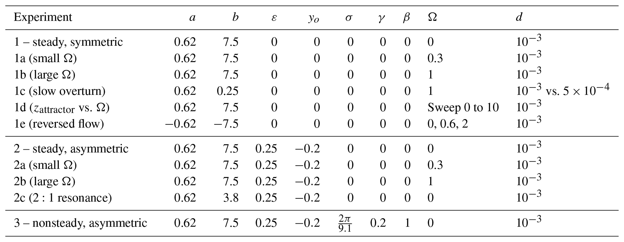
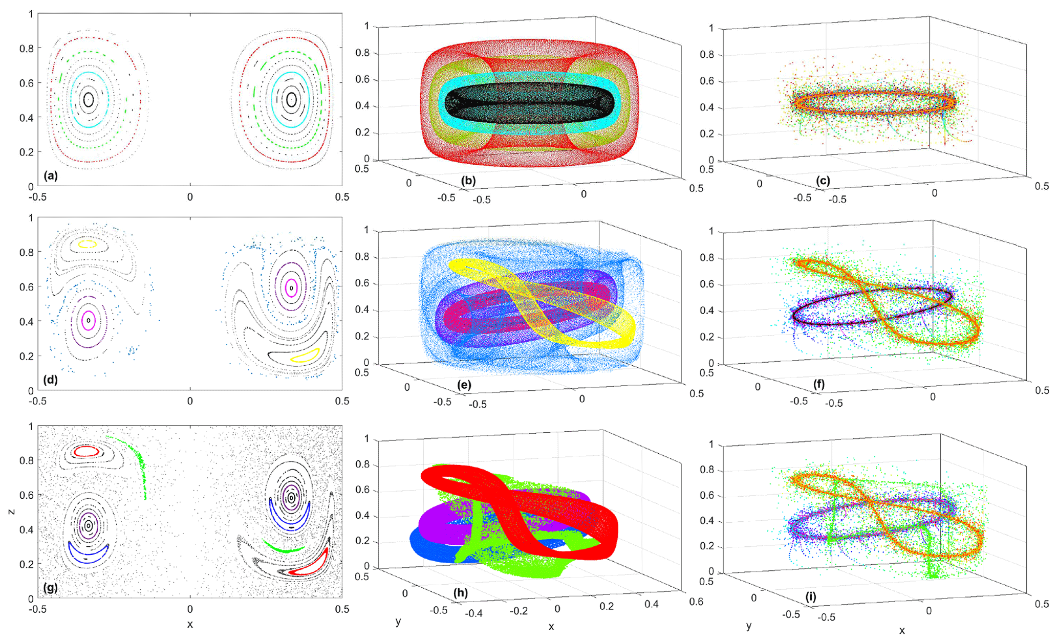
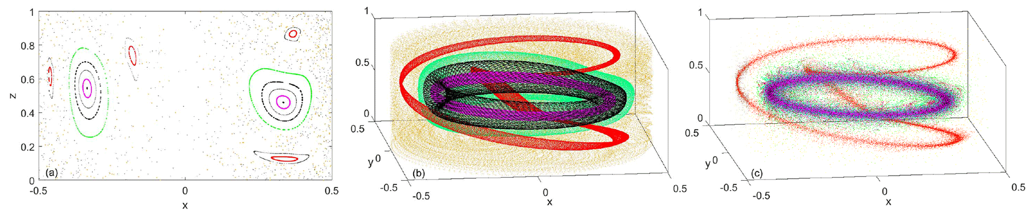
Figure 2(a, d, g) Poincaré section; (b, e, h) fluid parcel trajectories in 3D; (c, f, i) buoyant particle trajectories in 3D for a steady, symmetric fluid flow (a–c); buoyant particle trajectories in 3D for a steady, asymmetric flow (d–f); and buoyant particle trajectories in 3D for a nonsteady, asymmetric flow (g–i). Parameter setting are listed under Experiments 1, 2, and 3 in Table 1. Colors in panels in the left column match the corresponding panels in the middle column, but the colors in the panels in the right column indicate time after particle release. Note the attraction of buoyant particles to a single attractor at mid-depth in panel (c), to two attractors in panel (f), and to three attractors in panel (i). Particles are released along a vertical line x=0.334, y=0, and with an initial velocity equal to that of the co-located fluid parcels.
We now review the main features of the Lagrangian circulation in the rotating cylinder flow. In the steady, symmetric configuration, each fluid trajectory is confined to the surface of a torus as it winds around the cylinder. The typical torus is associated with quasiperiodic trajectories, and any such trajectory, followed for a sufficient length of time so that it completes many overturning and azimuthal rotations around the cylinder, will sketch out the torus in 3D. Figure 2b contains several examples of such tori, and Fig. 2a shows the corresponding Poincaré map, made by marking the crossing points of trajectories with a vertical slice through the cylinder. After a large number of crossings, each quasiperiodic trajectory traces out the cross-section of the torus on which it lives. The tori are nested within each another, with a single, horizontal, periodic trajectory located at the center of the nest. Certain tori contain periodic trajectories, and these will show up as a finite number of dots on the Poincaré map. Because of this geometry, the motion of fluid parcels is most naturally described in terms of action–angle–angle variables, where the action (I) acts a label for a particular torus and is constant following each trajectory, while the two angle variables ( and ϕ) define the location of a parcel on the torus. Here, is an azimuthal angle that differs from the above cylindrical coordinate θ in how its origin is defined, while the “poloidal” angle ϕ wraps around the cross-section of each torus. The coordinates are non-orthogonal but are defined in such a way that the angular velocities, and Ωϕ, are also constant following a trajectory. The explicit transformations to the action–angle–angle variables are given in Mezic and Wiggins (1994).
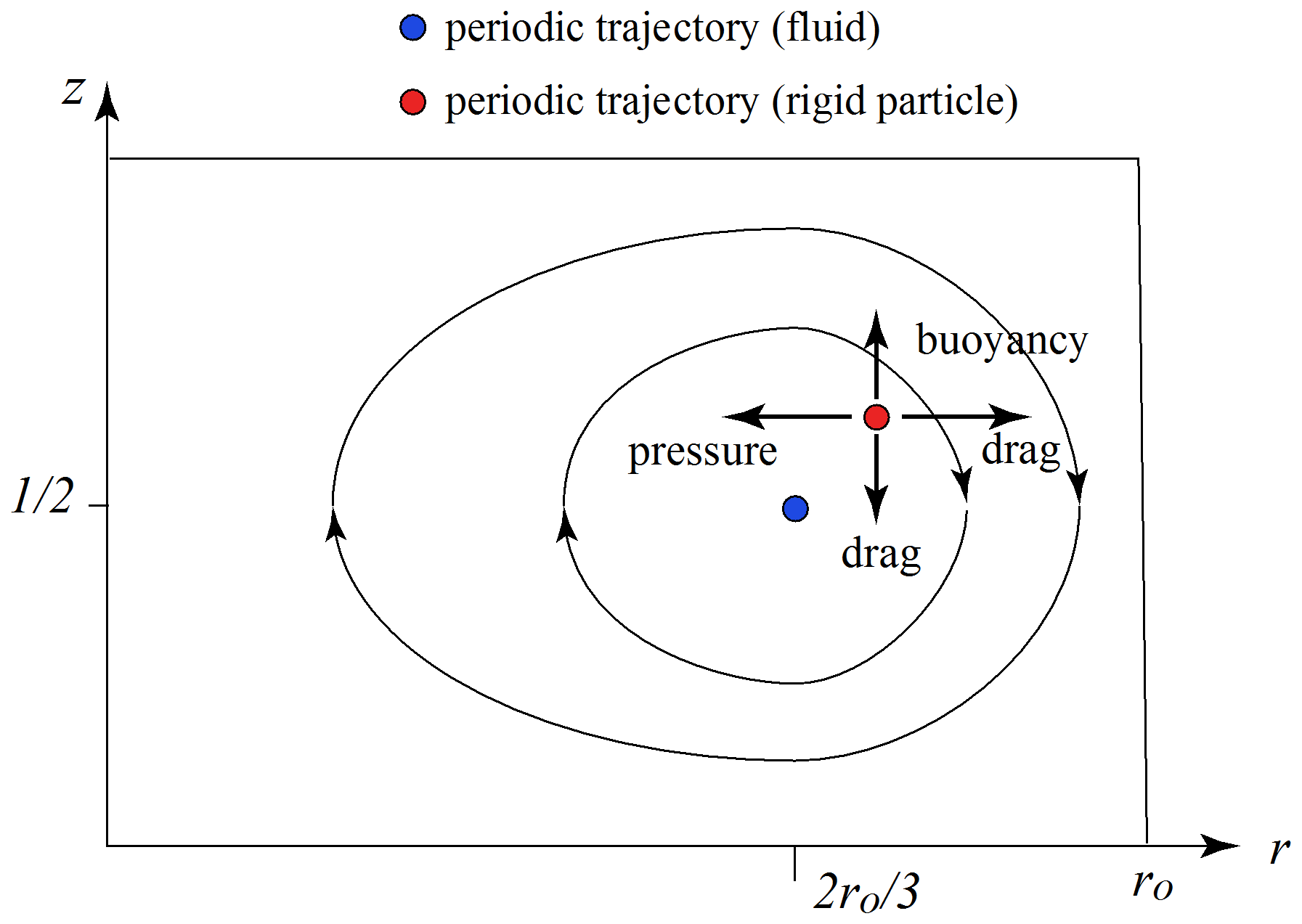
Figure 3Sketch showing the position in a vertical section of the periodic orbit (red dot) of the rigid particle relative to the periodic orbit (blue dot) of the fluid flow. The viewer sees one-half of a vertical slide though the cylinder, with the azimuthal flow directed away from the viewer and the cylinder center at the left edge.
When the symmetric rotating cylinder flow is perturbed by a small, steady, symmetry-breaking perturbation, as controlled by the parameters ε and yo in Eq. (9), the tori that are populated by periodic orbits potentially become resonant and break up, resulting in chaotic motion of fluid parcels in the vicinity (Fig. 2d–i). Tori with quasiperiodic orbits deform but stay intact. Examples are discussed by Fountain et al. (2000) and Pratt et al. (2014), and the latter publication found that chaos generally dominates in a large region that includes the central axis of the cylinder and extends around the boundaries of the cylinder. Away from this region, the space is occupied by tori that have survived the perturbation, and these are sandwiched between tori that have broken up and created braided regions of chaos. The breakup of a torus also gives rise to new tori that appear as islands in the Poincaré maps (Fig. 3d, g), and these contain non-chaotic trajectories. The number of islands can be predicted by a theory that decomposes the symmetry-breaking perturbation into Fourier modes, written in the () coordinates, with wave numbers n and m in the and ϕ directions, respectively. If the angular velocities and Ωϕ characterizing the trajectories on a particular torus satisfy the resonance condition for some n and m, equivalent to the trajectories on that torus being periodic, then that torus will break up and a new set of invariant tori (islands) will form. Running through the center of the islands will be a periodic trajectory that will execute n azimuthal cycles to every m poloidal (overturning) cycles. In the case shown in Fig. 3a, , so the periodic trajectory circles the cylinder horizontally once for each overturning cycle: a so-called 1:1 resonance.
If the symmetry-breaking perturbation is quasiperiodic in time, with underlying frequencies σi, the resonance condition for the breakup of a torus becomes , where li represents integers (Rypina et al., 2015). Unlike the resonance condition for the steady perturbation, which is only satisfied on tori foliated by periodic trajectories, this new resonant condition may be satisfied on tori that have quasiperiodic orbits, and the resonant islands that form will have a shape and location that vary in time. An example (Fig. 2g, h) of the case of a resonance with a single-frequency (i.e., temporally periodic) perturbation shows a number of resonant islands. These features vary in time, recovering their shape and location periodically, and the snapshots shown are obtained by strobing the trajectories in 3D and at the forcing frequency. The green and blue islands in Fig. 2h have resulted from the breakup of tori with quasiperiodic trajectories, and the center of the island corresponds to a closed material curve that is populated with quasiperiodic trajectories.
Note that the resonance condition above and our results in general are applicable to quasiperiodic disturbances with finite number of frequencies, rather than only periodic disturbances. (We only show numerical simulations for the temporally periodic case for simplicity.) Because any broad-spectrum function can be arbitrary closely represented by a quasiperiodic function with a finite number of frequencies, this could be applicable to some oceanic flows, especially those with pronounced peaks in the spectrum. However, for flows with a truly broadband spectrum, this approach is probably poorly applicable and/or at least impractical because of the very large number of discrete frequencies needed. This is similar in its utility/applicability to other Kolmogorov–Arnold–Moser-based and resonance-based arguments used in prior papers by many authors; see, for example, Rypina et al. (2007) and Beron-Vera et al. (2008, 2010).
Aggregation of rigid particles will occur in the presence of an attractor, an object with a dimension <3 to which particles tend asymptotically in time. We are most interested in attractors that occur in the interior of the rotating cylinder and that are set up by the background circulation, as opposed to the physical boundaries of cylinder. We will see that a closed material contour consisting of periodic orbits near the core of the nested tori in the steady, symmetric case act as an attractor for slightly buoyant particles and that similar material contours consisting of periodic or quasiperiodic orbits near the centers of the resonant islands in the asymmetric cases can play the same role. We will explore three cases in increasing complexity, beginning with steady flows with axial symmetry and proceeding to steady, asymmetric flows and finally unsteady, asymmetric flows.
The search for attractors is motivated by the hypothesis that, for cases of strong drag (where the rigid-particle velocity lies close to the fluid velocity), a periodic orbit for the rigid-particle motion will exist in the vicinity of a periodic trajectory for the fluid parcel motion and that, if Qa>0 in a region surrounding the latter, it should attract buoyant particles. For the time-dependent case, we extend the search to included closed loops that contain recirculating rigid particles and that vary periodically in time.
3.1 Steady, axially symmetric 3D flows
The fluid velocity field for this case is given by Eqs. (9c) and (10), and these indicate that the location of the horizontal, periodic fluid parcel trajectory living at the center of the nested tori is given by and . It is natural to ask whether a periodic trajectory for rigid particles also exists nearby. In the slow-manifold approximation, the steady radial, azimuthal, and vertical particle velocities are obtained by writing Eq. (4) in cylindrical coordinates, leading to the following:
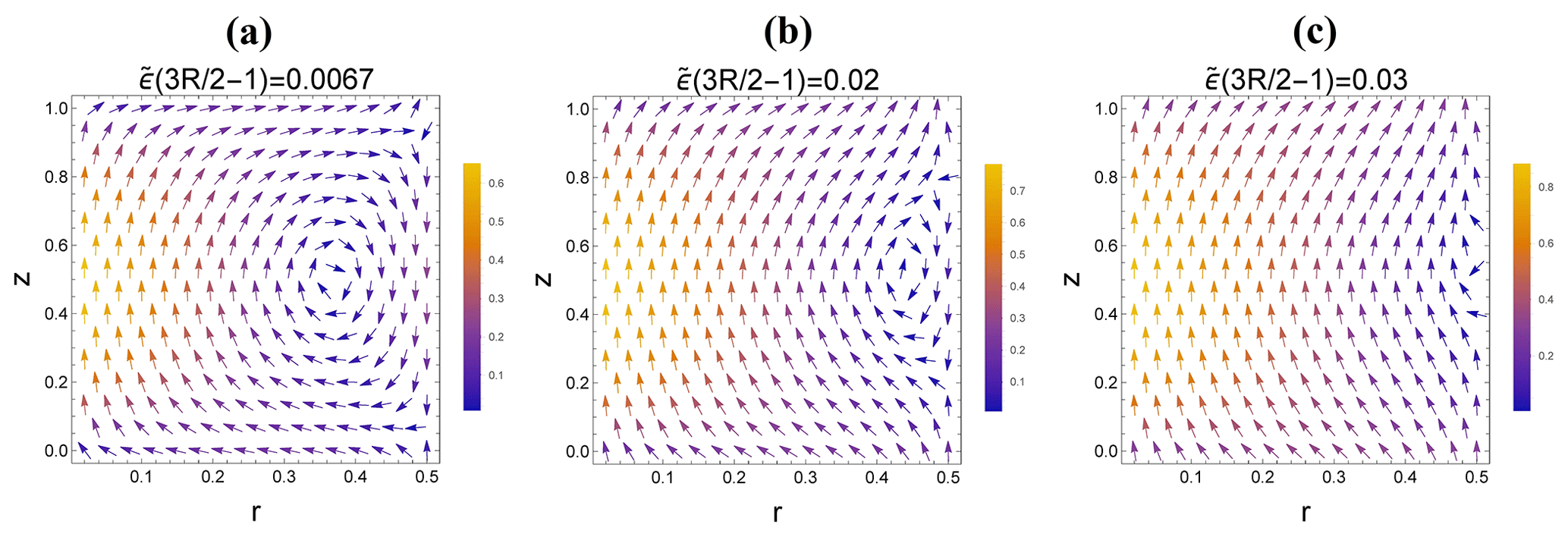
Figure 4The slow-manifold radial and vertical velocity components for the rigid particles, plotted in the r–z plane for (a) , (b) , and (c) . Other parameters are as listed for Experiment 1a in Table 1.
3.1.1 Position of attracting periodic orbit – approximate analytical expression on a slow manifold
Searching for points r=rc and z=zc for which and which lie in proximity to the horizontal trajectory of the flow, we introduce the following:
Substituting the above expressions into the right-hand sides of Eq. (11a, c) and setting both to zero results, after neglecting the terms, in the following:
and
For the parameters a>0 and b>0, circulation is cyclonic with upwelling in the center of the cylinder, and for buoyant particles, so the corrections are positive and the periodic particle orbit lies at a larger radius and elevation than the periodic fluid orbit. Note also from Eq. (11b) that the azimuthal velocity component of the rigid particle on the periodic orbit is equal to that of the fluid.
An explanatory sketch (Fig. 3) shows the position of the periodic orbit of the rigid particle relative to that of the periodic orbit of the fluid. As the rigid particle is buoyant, it can maintain its level z only if it is situated in a region where the vertical fluid velocity is <0, here to the right of the periodic orbit of the fluid flow. Also, the horizontal pressure gradients associated with the centripetal acceleration associated with the frame rotation (term Ω2r), the Coriolis acceleration (term 2Ωu(θ)), and the centripetal acceleration due to the azimuthal velocity are all positive for this flow, so that low pressure exists at r=0 and the rigid particle is forced horizontally inward. To remain stationary, the particle must sit in a region where the radial velocity of the fluid is outward. In this manner, the periodic trajectory exists at a location where the forces of inertia, buoyancy, and added mass can be countered by the drag due to the background flow. If we fix all other parameters and increase Ω through positive values, the term multiplying in Eq. (12b) will become dominated by the Ω2 term, will grow without bound, and the periodic trajectory may cease to exist. At the same time, a periodic orbit for the rigid particle can always be found close to that of the fluid, regardless of the magnitudes of the parameters Ω, a, b, etc., provided that the relative particle size (and thus and/or the relative density difference (and thus is made sufficiently small.
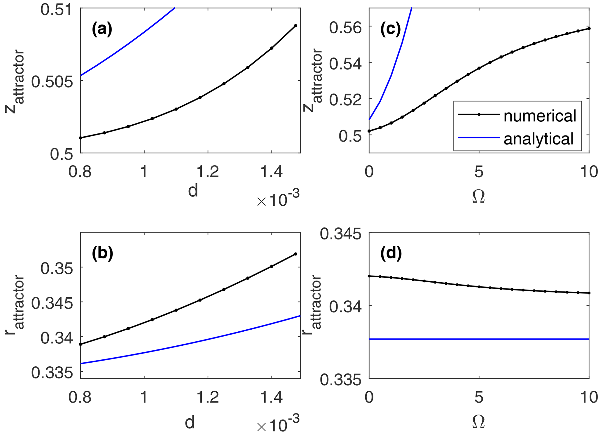
Figure 5For the steady, symmetric rotating cylinder flow, the coordinates of the periodic orbit that acts as an attractor for buoyant particles are shown as a function of particle diameter (a, b) and frame rotation (c, d). Flow parameters are listed in Table 1 and correspond to Experiment 1 for panels (a) and (b) and to Experiment 1d for panels (c) and (d).
3.1.2 Position of attracting periodic orbit – conditions for the loss of periodic orbit
We have suggested that periodic orbits for rigid particles are encouraged when the ; in the case of Run 1, this value is 0.0066. A cross-sectional plot of the radial and vertical components of the slow-manifold particle velocity in a vertical section through the cylinder (Fig. 4a) shows that the periodic orbit lies at r=0.369 and z=0.504 (as compared to the values of rc=0.338 and zc=0.502 predicted by Eq. 12). (The convergence of the surrounding velocity field is too weak to be seen in the graphic.) If is raised to the moderately small value of 0.02, the position of the periodic trajectory migrates towards a larger radius (Fig. 4b), with the reason for this being that the greater buoyancy (larger value of or smaller drag (larger ) requires a larger downward fluid velocity for equilibrium. As the maximum downward fluid velocity occurs at the outer cylinder wall (see Eq. 9c), the position of the periodic orbit continues to migrate outward and is lost (Fig. 4c) when exceeds a value close to 0.03.
3.1.3 Position of periodic orbit in numerical simulations
The slow-manifold reduction yields to the prediction (Eq. 12) of the position of the attracting material contour, or loop, for slightly buoyant particles. We can compare this prediction to what is observed in numerical simulations using the Maxey–Riley equations (Eqs. 1, 2) over a range of particle sizes d (and thus and frame rotations Ω. As shown in Fig. 5, qualitative agreement with the slow-manifold prediction, and the sketch in Fig. 3, holds for a very small d (when is small). Here, the attractor in Fig. 5 is located close to the central periodic fluid parcel trajectory that lives at mid-depth, z=0.5 and . As d (and ) increases, the attractor moves increasingly up and outward, and, although the theory captures the trends, quantitative agreement with the numerical results worsens. Also, when frame rotation Ω is increased (Fig. 5c), the attractor responds by shifting up from mid-depth, again in qualitative but not quantitative agreement with the slow-manifold prediction in Eq. (12b).
3.1.4 Geometry of rigid-particle trajectories and evidence of attraction in numerical simulations
If in the neighborhood of the periodic rigid-particle trajectory Qa >0, the phase space for buoyant particles will contract and the periodic trajectory becomes a candidate for an attractor of such particles. An example of the attraction towards the periodic orbit is shown in Fig. 2c, where a set of slightly buoyant particles have been initialized over the volume of the cylinder, and Eqs. (1) and (2) have been integrated forward in time to determine their subsequent trajectories. Each trajectory is shown using a unique color. It can be seen that the particles aggregate within a ring-like structure of decreasing thickness in the general vicinity of the periodic orbit of the fluid flow.
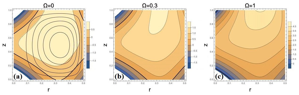
Figure 6(a) The Qa function for the steady, axisymmetric cylinder flow with the same parameter settings (see Experiment 1a) as for Fig. 3a–c and plotted in x–z along with the streamlines of the overturning circulation. The thick, rigid curve corresponds to Qa=0. Panel (b) shows the same parameter settings except that Ω has been raised from 0 to 0.3 (Rossby number ≅1). In panel (c), Ω=1.0 (Rossby number ≅0.2).
3.1.5 Basin of attraction – relationship to Qa
To map out the basin of attraction for the particle periodic orbit, we first consider the region over which phase space contraction for the buoyant particles (i.e., Qa>0) occurs. This region is shown in Fig. 6a for the current example, along with the streamlines of the fluid overturning stream function. Much of the fluid flow recirculates entirely within the region of positive Qa, whereas some of the outer streamlines cross the boundary (thick contour) between positive and negative Qa. If it were the case that rigid particles exactly followed streamlines of the fluid overturning circulation, then net contraction or expansion of phase space along a rigid-particle trajectory would depend on the sign of the time-integrated value of Qa along streamlines. The Qa=0 contour, shown by a bold contour in each frame of Fig. 6, might then approximately delineate the basin of attraction for buoyant, rigid particles. In the slow-manifold approximation, where rigid-particle velocities lie close to the fluid velocities, the Qa=0 contour might continue to do so.
To test this conjecture, we locate the basin of attraction in the numerical simulations by releasing buoyant particles at various locations in the cross-section and , integrating the subsequent trajectories over many overturning cycles, and recording the position (xfinal and zfinal) of each particle where it crosses the same plane the final time (i.e., recording final crossing with the Poincaré section). We use the variable-step fourth-order Runge–Kutta integration scheme, which we implemented in MATLAB via the built-in “ode45” function. In our simulations, the relative and absolute tolerances are set to the value of 10−9 to integrate particle trajectories (Eqs. 2, 3) (our results were not sensitive to the further decrease in tolerance values). As the flow (Eq. 9a, b, c) is prescribed analytically and has no normal flow component at the perimeter and top and bottom of the cylinder, no interpolation scheme is needed and no extra boundary conditions are enforced during the integration. Integration of a trajectory is stopped when a particle gets within one particle radius of the cylinder walls or top/bottom. The values of zfinal as a function of initial particle position are mapped in Fig. 7a, where the large green area corresponding to zfinal≅0.5 indicates the region from which particles are attracted. Only particles initiated near the central axis of the cylinder and close to the cylinder boundaries lie outside this region, and these rise to the surface of the cylinder, contact the upper lid, and are no longer followed. It can be seen that the green area in Fig. 7a has an oval shape that somewhat resembles the overturning streamlines at small x in the central part of the cylinder, but it extends to near the top, bottom, and outer cylinder boundaries at larger x. Thus, the Qa=0 contour provides a rough indication of the size and shape of the basin of attraction, although it misses some important details.
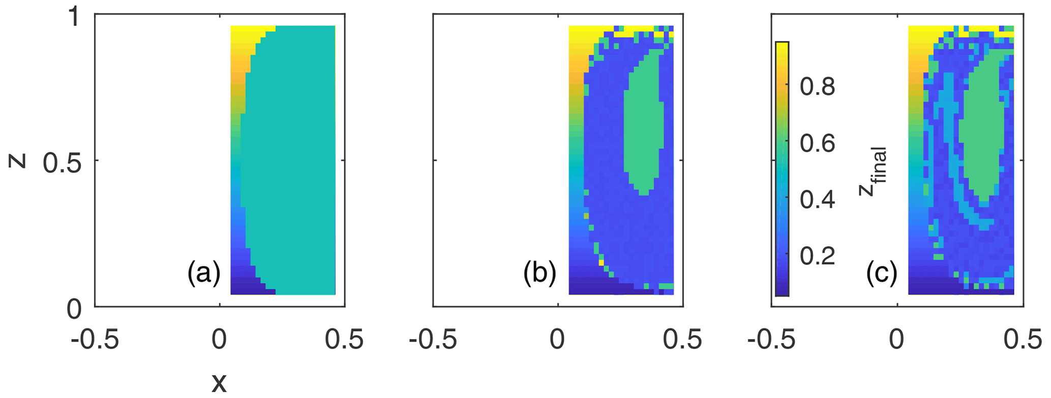
Figure 7Domain of attraction for the attractors in (a) steady, symmetric (Experiment 1 in Table 1); (b) steady, asymmetric (Experiment 2 in Table 1); and (c) temporally periodic, asymmetric rotating cylinder flow (Experiment 3 in Table 1). (These are the same three experiments that were used to produce Fig. 2.) The color indicates the height (i.e., value of the z coordinate) of the final crossing of a trajectory with the Poincaré section, as a function of the particle's release location. Thus, particles attracted to the same attractor correspond to the same color.
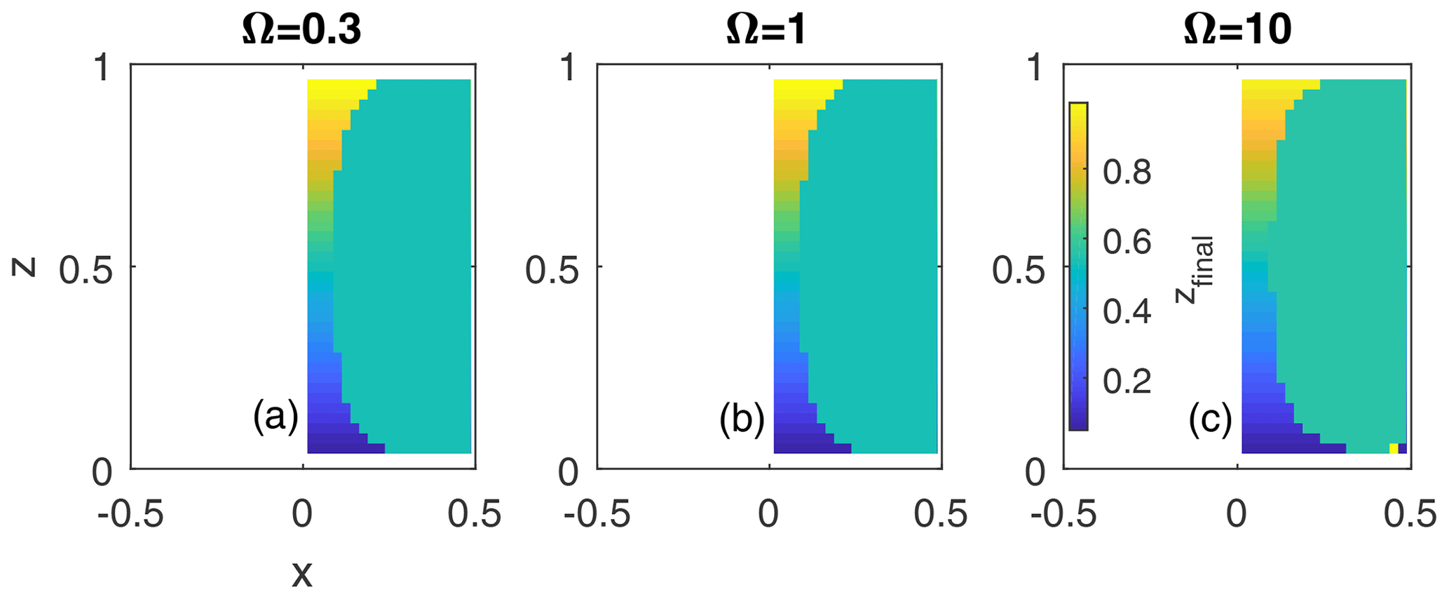
3.1.6 Basin of attraction – dependence on Ω
We have seen that the location of the periodic orbit that acts as an attractor for buoyant particles shifts up and out in response to increasing frame rotation Ω (Fig. 5c). In Fig. 8, we indicate the corresponding changes in the extent of the basin of attraction with respect to changing Ω by recomputing Fig. 8a with Ω=0.3, 1, and 10, respectively. The two smaller Ω values (0.3 and 1) correspond roughly to Rossby numbers of about 1 and 0.2, i.e., are representative of the ocean submesoscale and mesoscale flows. The Qa functions for these cases are plotted in Fig. 6b and c, respectively. Most submesoscale eddies are going to tend to have of about the same magnitude as Ω (except on the Earth's Equator) and mesoscale eddies will have . The results in Fig. 8 suggest that, while the basin of attraction does shrink slightly with increasing Ω, this dependence is weak. The main difference between the three numerical runs in Fig. 8 is in the associated attraction time, which gets significantly shorter for larger values of Ω. This is explored in more detail below.
3.1.7 Attraction time
It follows from Eq. (6) that the attraction time towards the periodic orbit should scale as , where with . Thus, for ζr≥0, as in most of our numerical runs (except Experiment 1e), attraction time decreases with increasing Ω for positive Ω≥0. For negative ζr, which corresponds to the reversed direction of the flow in our simulations (Experiment 1e), an increase in Ω will initially slow the attraction by decreasing the magnitude of ζa all the way to 0, at which point the periodic orbit will lose its attraction properties, but will then speed up the attraction as Ω is further increased. This trend is confirmed numerically in Fig. 9, where, for the flow parameters corresponding to the “reversed flow” run in Table 1 (Experiment 1e, with ζr<0), we release a sample trajectory within the basin of attraction and plot its z coordinate as it winds around the can and eventually approaches the attracting periodic orbit. As anticipated, the attraction time initially increases as Ω is increased from to 0.6 but then decreases as Ω is further increased to 2.
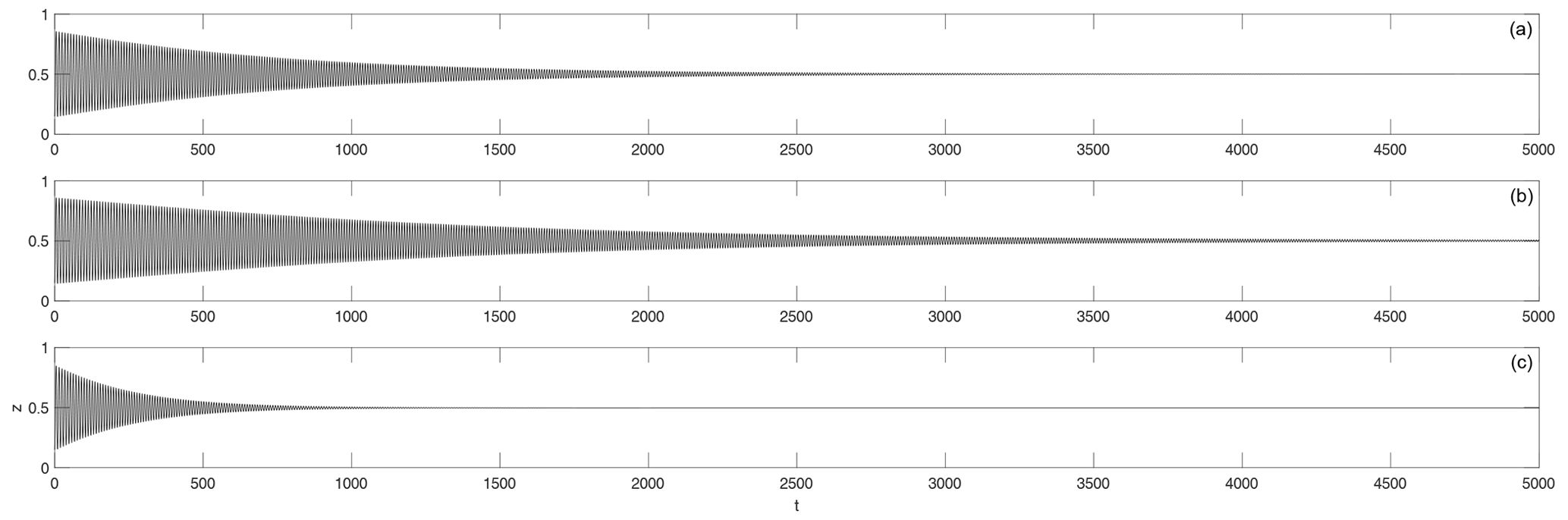
Figure 9For the “reversed flow” experiment (Experiment 1e in Table 1), the z position of a sample particle trajectory is shown as function of time for three values of Ω: 0 (a), 0.6 (b), and 2 (c). Time t is in dimensionless units (but as our scaling coefficient for time is equal to 1 s, the numbers on the x axis can also be read as dimensional time in seconds).
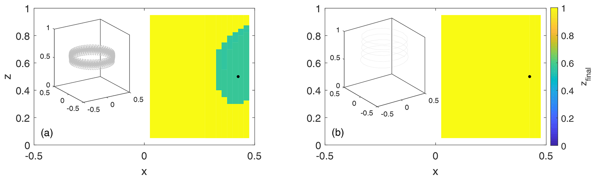
Figure 10For the “slow overturn” Experiment 1c from Table 1, the color indicates the final z coordinate of a particle's trajectory at the end of the integration time as a function of the particle's release location for two values of d: (a) and (b) 10−3. Yellow corresponds to particles rising up to the top, whereas green indicates the basin of attraction of the subsurface attracting periodic orbit. The insets on the left-hand side of each frame show a sample trajectory whose release location is indicated by the black dot.
3.1.8 Disappearance of the subsurface attractor when becomes too large
Finally, to illustrate the disappearance of the subsurface attractor when becomes too large, we contrast two numerical simulations with the same flow parameters (corresponding to the “slow overturn” run 1c in Table 1) but different particle diameters, vs. (in Fig. 10). For larger d, the subsurface periodic orbit for rigid particles is no longer present within the can, leading to all particles rising up to the surface (Fig. 10b). For smaller d, the periodic orbit is still present and acts as an attractor for buoyant, rigid particles over a significant portion of the can (green region in Fig. 10a). We note that this run would be more qualitatively similar to the oceanic mesoscale or submesoscale eddies, where the overturning component of circulation is weak in comparison to the horizontal swirl.
3.2 Steady, non-symmetrically perturbed case
We now consider a case in which the axial symmetry of the steady flow has been broken, here via a change in the perturbation amplitude parameter ε from 0 to 0.25 and via a change in the offset parameter yo from 0 to −0.2 in Eq. (9a, b). The fluid velocity field now contains something like a stationary, “mode-1” azimuthal wave in the horizontal velocity field.
The resulting Lagrangian structure (Fig. 2d, e) has a sea of chaos that covers the near-axial and outer regions of the cylinder, where no unbroken tori survive. Within this chaotic sea is a region containing a nest of unbroken tori that surround a central periodic orbit. This orbit has evolved from the central periodic orbit of the symmetry case and is now tilted. Within the nest of unbroken tori there exist resonant layers, in which new tori have arisen, and the most prominent is the “island” that is centered near x=0.4 and z=0.2 in the right half (and near and z=0.8 in the left half) of Fig. (2d). We further note that this center lies within the region of positive Qa (Fig. 6b). The island corresponds to the yellow tori in Fig. 3e and is produced by a 1:1 resonance, so that the periodic trajectory running through its center executes one complete azimuthal cycle and one overturning cycle before connecting back onto itself. Thus, in this steady, asymmetric configuration, we now have two periodic orbits of the fluid flow: the central slightly tilted periodic orbit near mid-depth (that evolved from the central horizontal periodic orbit of the axisymmetric flow) and a new periodic orbit running through the center of the resonant island (resulting from the breakup of the resonant torus satisfying .
We speculate that, for sufficiently small , a periodic orbit for the rigid-particle motion exists in the vicinity of each of the two periodic orbits of the fluid flow. This conjecture is difficult to prove due to a complex geometry, leading to centrifugal forces that act in different directions at different locations along the particle path. For now, we simply search for the supposed attractors by releasing particles and following their trajectories.
As shown in Fig. 2f, separate attractors arise in the vicinity of two periodic orbits. The first appears as a ring-like structure (purple core) lying near the center of the original nested tori and the second is a similar feature with a red core near the center of the resonant island. The two are chained together, and each has its own basin of attraction (Fig. 7b): the first consisting of a roughly elliptical patch (inner green region) in the x–z plane, which corresponds of a slice through a tube-like structure in 3D, and the second consisting of an annular (blue) region that surrounds the green region and that occupies a relatively larger volume.
In order to check that the attraction of slightly buoyant, rigid particles towards periodic orbits located near the centers of the resonant islands in the perturbed flow is not limited to the case of the 1:1 resonance, we adjusted the background flow parameter b in Eq. (9), which is responsible for the overturning strength, in an additional simulation (Fig. 11, experiment 2c in Table 1) to create a 2:1 resonance instead of a 1:1 resonance, as in the original run. In this case, the resonant torus breaks down giving rise to a two-island chain on the corresponding Poincaré section (Fig. 11a), and the fluid periodic orbit that goes through the centers of both islands completes two full cycles in azimuth and one complete cycle in vertical before connecting onto itself. Also, as in the original run, a second slightly tilted periodic orbit still exists near mid-depth of the can. When buoyant particles are released into this flow, two attractors arise, corresponding to the two periodic orbits of rigid particles: one near mid-depth (purple core in Fig. 11c) and another in red near the center of the 2:1 resonant island.
3.2.1 Shift in the position of the periodic orbit associated with a resonant island as a function of flow and particle parameters as well as frame rotation
The position of the attracting periodic orbit for rigid particles that is located within the resonant islands (referred to as the resonant periodic orbit hereafter) in the asymmetrically perturbed flow depends on the perturbation strength (via ε), the flow and particle parameters (via ), and the frame rotation Ω. Specifically, this resonant periodic orbit for the rigid particles will shift away from the corresponding periodic trajectory of the fluid flow as and Ω are increased. The same is true for the slightly tilted central attracting periodic orbit near mid-depth. This is qualitatively similar to the shifting of the central periodic orbit up and out from z=0.5, r=0.34 in the axisymmetric flow in response to changing and Ω, which we explored in detail in the previous section, both analytically (Eq. 12) and numerically (Figs. 3–5).
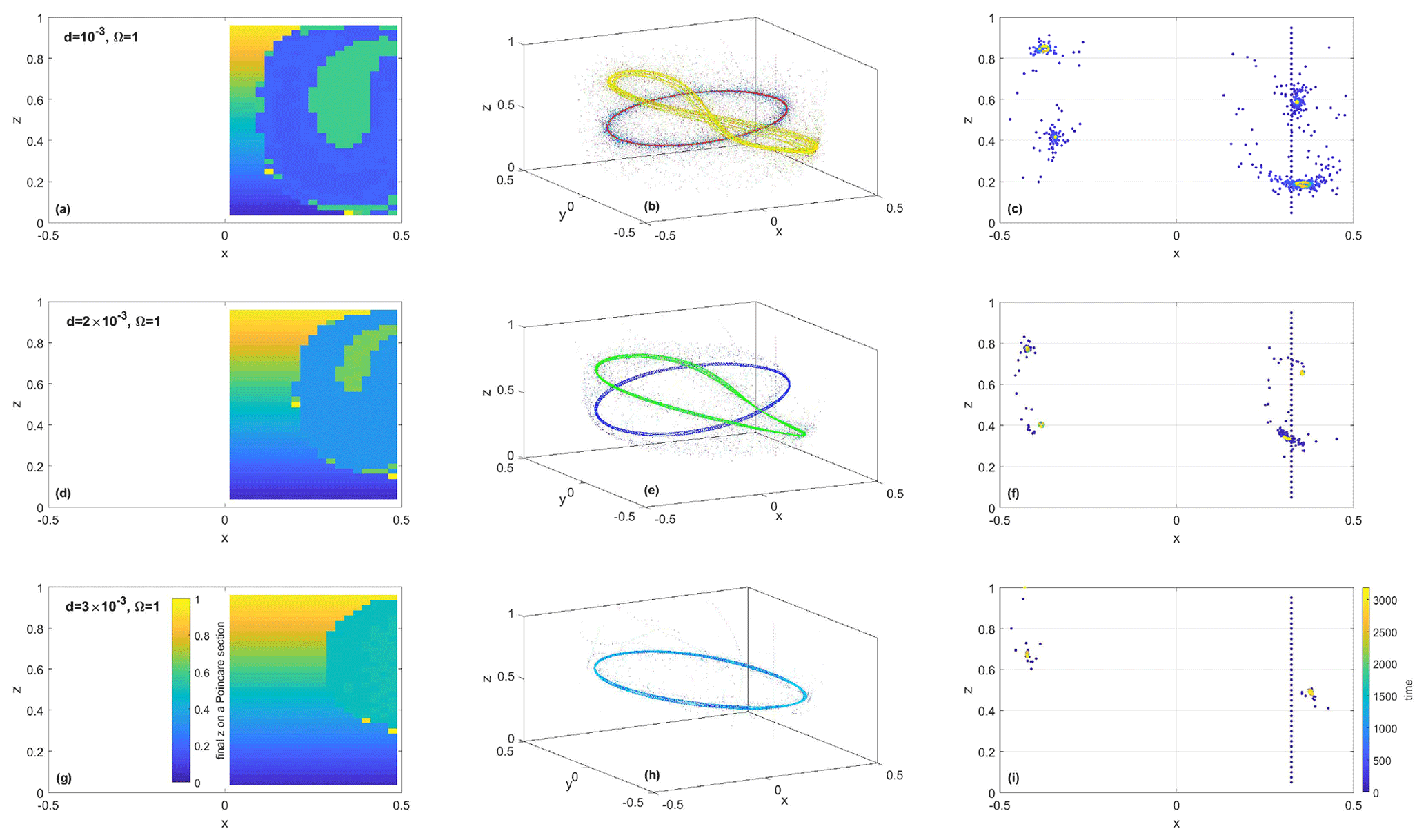
Figure 12For the steady, perturbed system (Experiment 2 in Table 1), changes in the location of the attracting periodic orbits, basins of attractions, and time of attraction are shown as a function of particle diameter d (and thus ). Panels (a), (d), and (g) show the z coordinate of the last crossing of the trajectory with the x–z Poincaré plane as a function of release location; flat regions are basins of attraction for the two attractors. Panels (b), (e), and (h) show 20 trajectories in 3D released along a vertical line at y=0, x=0.334, and ; denser cores indicate attractors. Panels (c), (f), and (i) show the crossing of the same select 20 trajectories with the x–z Poincaré plane, color-coded by time: blue corresponds to release location and yellow corresponds to final positions.
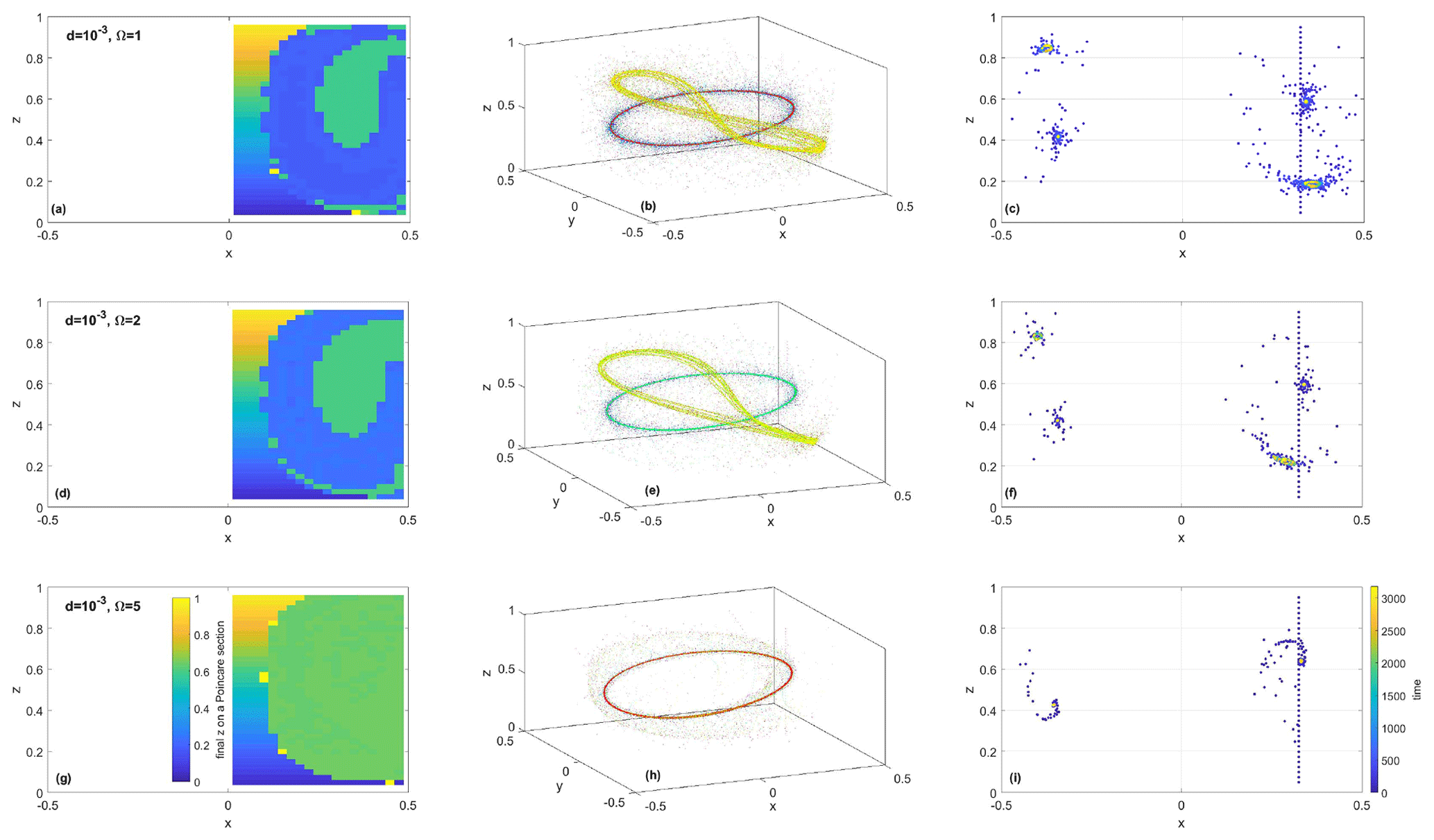
Figure 13For the steady, perturbed system (Experiment 2 in Table 1), changes in the location of the attracting periodic orbits, basins of attractions, and time of attraction are shown as a function of frame rotation Ω. Panels (a), (d), and (g) show the z coordinate of the last crossing of the trajectory with the x–z Poincaré plane as a function of release location; flat regions are basins of attraction for the two attractors. Panels (b), (e), and (h) show 20 select trajectories in 3D released along a vertical line at y=0, x=0.334, and ; denser cores indicate attractors. Panels (c), (f), and (i) show the crossing of the same 20 trajectories with the x–z Poincaré plane, color-coded by time: blue corresponds to release location and yellow corresponds to final positions.
In order to numerically illustrate the shift in the position of the attracting periodic orbits, we present (Figs. 12, 13) numerical simulations in the steady, perturbed flow configuration for three values of d (and thus ) and three values of Ω. As both parameters increase, the attractors move away from the corresponding periodic orbits of the fluid flow. This shift is evident from the change in the color of the attraction basins in panels (a), (d), and (g) and from the location of the yellow cloud of dots in panels (c), (f), and (i) in Figs. 12 and 13. Increases in and Ω also lead to the shrinkage of the attraction basins for both attractors and to a faster convergence rate, as is evident from the tighter cloud of yellow dots in panels (c), (f), and (i), as discussed in more detail below. The basin of attraction for the central attractor – the green region in Fig. 12 – seems to shrink faster than the basin of attraction for the resonant attractor (the blueish region) as d increases, so when d is increased from to , the central attractor vanishes, whereas the resonant attractor is still present (Fig. 12g). On the other hand, the increase in Ω (Fig. 13) causes a faster shrinkage of the basin of attraction for the resonant attractor than for the central attractor, so when Ω is increased from 2 to 5 in Fig. 13g, the resonant attractor disappears, whereas the central attractor is still present. Figure 12g, h, and i (and Fig. 13g, h, and i) show cases where this threshold has been exceeded, and one of the attractors has been lost, whereas the other is still present.
3.2.2 Attraction time
Similar to the unperturbed flow, the attraction time for attractors in the steady, perturbed flow may still scale as , provided that Qa is regarded as a typical value within the corresponding basin of attraction. The predicted decrease in attraction time with increasing and Qa is evident from the numerical simulations in panels (c), (f), and (i) in Figs. 12 and 13, where we color-coded the trajectory crossings with the x–z Poincaré plane by time, with blue (yellow) corresponding to initial (final) time. For smaller values of and Ω, we observe a wider and more diffuse cloud of dots (because trajectories wind around the can many times before approaching the attractor), whereas the clouds at comparable times become denser and more compact around the attractors as and Ω increase.
3.2.3 Basin of attraction
For the slightly tilted central periodic orbit located within the central non-chaotic region near mid-depth in Fig. 2f, we observe that the basin of attraction – green region in Fig. 7b – extends roughly from the location of the periodic orbit to the edge of the central non-chaotic region (that is foliated by discretely sampled closed curves in Fig. 2d). Note that, as increases, the attracting periodic orbit moves away from the center of this non-chaotic region towards its edge, leading to the shrinkage and eventual disappearance of the corresponding basin of attraction (shown by the green regions in Fig. 12a, d, and g).
Similarly, in all of our numerical simulations, we observe that, for the resonant attracting periodic orbit running through the resonant islands, the basin of attraction seems to cover the region between the orbit and the edge of the corresponding resonant island. An analytical expression for the width of the (non-degenerate) resonant island in the fluid flow (Pratt et al., 2014) predicts that , where ΔI is the deviation in the action coordinate away from I0, the value of action at the resonant torus (i.e., at the center of the island). This width depends on the strength of the perturbation ϵ, the order of the resonance (via n and m in the resonance condition), the background flow (via , and the structure of the perturbation (via . This expression could be used as an upper limit on the extent of the basin of attraction. However, because the attracting periodic orbit will move away from the center of the island towards its edge as and Ω increase, the basin of attraction for the resonant attractor (blue regions in panels a and d of Figs. 12 and 13) becomes increasingly smaller than ΔI. One might then speculate that the attractor will completely disappear when the attracting periodic orbit reaches the edge of the resonant island. This is the case in Fig. 13g, where the resonant attractor is no longer present.
3.3 Nonsteady, non-symmetrically perturbed case
The final case that we will consider is one in which the perturbation is asymmetric and varies periodically in time. The chosen perturbation frequency, , causes two strong additional resonances (compared with the steady, perturbed case): one with n=0, m=1, and l=1 (i.e., with a torus whose overturning frequency is equal to the perturbation frequency) that is shown in blue in Fig. 2g and h and is located near the outer edge of the central non-chaotic region and another (shown in green in Fig. 2g and h) with n=1, m=1, and l=1 that is located between the central non-chaotic region and the larger n=1 and m=1 resonant island (which was present in the steady case as well). Both of these new resonant structures are time dependent, with their shape and position recurring periodically. For example, the blue island, which looks like a crescent moon pointing upward on the Poincaré section at t=0, becomes a crescent moon pointing downward at time 4.55. The movement of the green island is more complex, as it turns both in the azimuth and vertical directions, making one complete loop over 9.1 time units. Because of the time dependence, trajectories must be strobed at the forcing frequency σ in order to capture “snapshots” of their forms as they recur at a particular phase in the time cycle. At the center of each feature is a closed material curve that also varies periodically. Where the island has emerged from the breakup of a torus with quasiperiodic orbits, the individual trajectories that populate the material curves are themselves quasiperiodic.
Particle trajectory computations in this case confirm that the purple, red, and green islands give rise to attractors (Fig. 3i), whereas the blue island does not. In fact, slightly buoyant, rigid particles that are released in the blue region converge towards the attractor that lies near the purple region. This is also indicated by the basin of attraction of the central attractor extending across the space occupied by the blue resonant island in Fig. 7c.
We have considered attraction phenomena for small, finite-size, spherical, buoyant, rigid particles in a 3D rotating cylinder flow with azimuthal rotation and overturning as well as with or without time dependence. The aim has been to gain insights into the behavior of slightly buoyant microplastic particles in 3D vortex flows that qualitatively resemble ocean eddies. The rigid-particle motion is governed by a simplified version of the Maxey–Riley equations (accounting for inertia, buoyancy, and simplified quantification of drag and added mass) and, approximately, by the slow-manifold reduction of these equations. We have illustrated the possibility of the aggregation of slightly buoyant, rigid particles in 3D vortex flows towards closed-loop attractors located in the subsurface region within the interior of the flow. Even in our idealized flow and for spherical particles with a fixed radius and buoyancy, aggregation is nontrivial, often with multiple attractors present and/or lack of attraction in some circumstances.
Our rotating cylinder model is much less complex than any real ocean eddy in many respects, including the assumed quasiperiodic time dependence and the absence of decay and interaction with the surroundings. Understanding aggregation in a simple periodic flow seems like a reasonable first step towards understanding aperiodic, interacting, and decaying oceanic eddies. This approach is common in applications of dynamical systems theory to oceanography and meteorology. For example, arguments relating to the increased stability of jets due to the strong Kolmogorov–Arnold–Moser stability near shearless trajectories were first developed for spatially periodic and temporally quasiperiodic flows and tested using idealized toy models before these ideas were explored in more realistic oceanic and atmospheric settings (see Rypina et al., 2007; Beron-Vera et al., 2008, 2010). Note also that our results are applicable to quasiperiodic disturbances with a finite number of frequencies rather than just periodic disturbances (we only show numerical simulations for the temporally periodic case for simplicity), and a quasiperiodic function might potentially be useful for approximating temporal variability in some oceanic flows, especially those with pronounced peaks in the spectrum.
We have explored a steady, axisymmetric rotating cylinder flow and a steady flow with its axial symmetry broken. In all cases, we have observed the emergence of subsurface attracting structures that lead to the aggregation of buoyant particles towards them. We have linked these attractors to the periodic orbits of rigid particles that exist in a region of net contraction of the phase space of the particle motion. The slow-manifold equations suggest that periodic orbits for rigid particles exist near periodic orbits of the underlying fluid flow, provided the drag is sufficiently strong (Stokes number ≪1).
We have also explored one case of an axially asymmetric and temporally periodic flow, with a focus on the resonant “islands” that arise due to the time dependence. At the center of such islands are closed material contours, or loops, composed of quasiperiodic orbits of the fluid flow. One such structure has a nearby attractor, also a closed loop of quasiperiodic orbits for rigid particles, while a second example does not. A detailed explanation awaits the formulation of a quantitative theory, something that is beyond the scope of the present paper and that will be presented in future work.
We have observed that the disappearance of an attractor, which can occur as the result of increasing rigid-particle size or frame rotation, coincides roughly with the displacement of the position of the attractor to the outer edge of the resonant island from which it sprang. Whether this purely geometric observation forms the basis for a general criterion for the loss of attraction is unknown, as a dynamical justification is needed.
Marine microplastics can have complex nonspherical, tangled-filament shapes; change their physical and chemical properties in time due to aging and photodegradation or chemical decay processes (Andrady 2011); are subject to biofouling (see recent relevant work by Kreczak et al., 2021); and may interact leading to the formation of clusters. None of these effects were considered in this paper, and all will need to be taken into account for the realistic prediction of marine microplastic evolution and redistribution in the ocean. Real ocean eddies are also decaying in time and are usually moving (translating) rather than stationary. Translation with a constant velocity can be handled by considering the flow in a moving frame of reference, but decay and interactions will likely change the geometry of the circulation and make the flow truly aperiodic. Our simplified model cannot account for these effects, which will need to be explored separately later.
No observational data were used in this work.
The supplement related to this article is available online at: https://doi.org/10.5194/npg-31-25-2024-supplement.
IIR led the overall effort and performed most of the numerical simulations, LJP contributed towards the theoretical understanding and interpretation of the results, and MD participated in the overall effort.
The contact author has declared that none of the authors has any competing interests.
Publisher's note: Copernicus Publications remains neutral with regard to jurisdictional claims made in the text, published maps, institutional affiliations, or any other geographical representation in this paper. While Copernicus Publications makes every effort to include appropriate place names, the final responsibility lies with the authors.
This research has been supported by the National Science Foundation (grant no. OCE 2124210) and the Office of Naval Research (CALYPSO grant nos. N000141812417 and N000141812165). We thank the reviewers for their helpful input.
This research has been supported by the National Science Foundation (grant no. OCE 2124210) and the Office of Naval Research (grant nos. N000141812417 and N000141812165).
This paper was edited by Vicente Perez-Munuzuri and reviewed by Erik van Sebille and Francisco Beron-Vera.
Andrady, A. L.: Microplastics in the marine environment, Marine Pollut. B., 62, 1596–1605, 2011.
Basset, A. B.: Treatise on Hydrodynamics, Deighton Bell, London, vol. 2, chap. 22, 285–297, 1988.
Beron-Vera, F. J.: Nonlinear dynamics of inertial particles in the ocean: From drifters and floats to marine debris and Sargassum, Nonlin. Dynam., 103, 1–26, 2021.
Beron-Vera, F. J., Brown, M. G., Olascoaga, M. J., Rypina, I. I., Kocak, H., and Udovydchenkov, I. A.: Zonal jets as transport barriers in planetary atmospheres, J. Atmos. Sci., 65, 3316–3326, 2008.
Beron-Vera, F. J., Olascoaga, M. J., Brown, M. G., Kocak, H., and Rypina, I. I.: Invariant-tori-like Lagrangian coherent structures in geophysical flows, Chaos, 20, 017514, https://doi.org/10.1063/1.3271342, 2010.
Beron-Vera, F. J., Olascoaga, M. J., and Lumpkin, R.: Inertia-induced accumulation of flotsam in the subtropical gyres, Geophys. Res. Lett., 43, 12228–12233, https://doi.org/10.1002/2016g1071443, 2016.
Beron-Vera, F. J., Olascoaga, M. J., and Miron, P.: Building a Maxey-Riley framework for surface ocean inertial particle dyamics, Phys. Fluids, 31, 096602, https://doi.org/10.1063/l.5110731, 2019.
Boussinesq, J.: Theorie Analytique de la Chaleur, L'Ecole Polytechnique, Paris, vol. 2, p. 224, 1903.
Brandt, L. and Coletti, F.: Particle-Laden Turbulence: Progress and Perspectives, Ann. Rev. Fluid Mech., 54, 159–189, https://doi.org/10.1146/annurev-fluid-030121-021103, 2022.
Choy, C. A., Robison, B. H., Gagne, T. O., Erwin, B., Firl, E., Halden, R. U., Hamilton, J. A., Katija, K., Lisin, S. E., Rolsky, C., and Van Houtan, S. K.: The vertical distribution and biological transport of marine microplastics across the epipelagic and mesopelagic water column, Sci. Rep., 9, 7843, 2019.
Daitche, A. and Tél, T.: Memory effects are relevant for chaotic advection of inertial particles, Phys. Rev. Lett., 107, 244501, 2011.
Delandmeter, P. and van Sebille, E.: The Parcels v2.0 Lagrangian framework: new field interpolation schemes, Geosci. Model Dev., 12, 3571–3584, https://doi.org/10.5194/gmd-12-3571-2019, 2019.
DiBenedetto, M. H. and Ouellette, N. T.: Preferential orientation of spheroidal particles in wavy flow, J. Fluid Mech., 856, 850–869, 2018.
DiBenedetto, M. H., Ouellette, N. T., and Koseff, J. R.: Transport of anisotropic particles under waves, J. Fluid. Mech., 837, 320–340, https://doi.org/10.1017/jfm.2017.853, 2018.
Faxén, H.: Der Widerstand gegen die Bewegung einer starren Kugel in einer zähen Flüssigkeit, die zwischen zwei parallelen ebenen Wänden eingeschlossen ist, Annalen der Physik, 373, 89–119, 1922.
Fenichel, N.: Geometric singular perturbation theory for ordinary differential equations, J. Differ. Equ., 31, 51–98, 1979.
Fountain, G. O., Khakhar, D. V., Mezić, I., and Ottino, J. M.: Chaotic mixing in a bounded three-dimensional flow, J. Fluid Mech., 417, 265–301, 2000.
Gatignol, R.: The Faxén formulae for a rigid particle in an unsteady non-uniform Stokes flow, 1983.
Greenspan, H. P.: The theory of rotating fluids (Vol. 327), 1st edn., Cambridge University Press, Cambridge, ISBN-10 0962699802, ISBN-13 978-0521051477, 1968.
Haller, G. and Sapsis, T.: Where do inertial particles go in fluid flows?, Physica D, 237, 573–583, 2008.
Hart, J. E. and Kittelman, S.: Instabilities of the sidewall boundary layer in a differentially driven rotating cylinder, Phys. Fluids, 8, 692–696, 1996.
Kaiser, D., Kowalski, N., and Waniek, J. J. Effects of biofouling on the sinking behavior of microplastics, Environ. Res. Lett., 12, 124003, https://doi.org/10.1088/1748-9326/aa8e8b, 2017.
Kelly, R., Goldstein, D. B., Suryanarayanan, S., Tornielli, M. B., and Handler, R. A.: The nature of bubble entrapment in a Lamb-Oseen vortex, Phys. Fluids, 33, 061702, https://doi.org/10.1063/5.0053658, 2021.
Kooi, M., Reisser, J., Slat, B., Ferrari, F. F., Schmid, M. S., Cunsolo, S., Brambini, R., Noble, K., Sirks, L. A., Linders, T. E., and Schoeneich-Argent, R. I.: The effect of particle properties on the depth profile of buoyant plastics in the ocean, Sci. Rep., 6, 33882, https://doi.org/10.1038/srep33882, 2016.
Kreczak, H., Willmott, A. J., and Baggaley, A. W.: Subsurface dynamics of buoyant microplastics subject to algal biofouling, Limnol. Oceanogr., 66, 3287–3299, 2021.
Kukulka, T., Proskurowski, G., Morét-Ferguson, S., Meyer, D. W., and Law, K. L.: The effect of wind mixing on the vertical distribution of buoyant plastic debris, Geophys. Res. Lett., 39, L07601, https://doi.org/10.1029/2012GL051116, 2012.
Kvale, K., Prowe, A. F., Chien, C. T., Landolfi, A., and Oschlies, A.: The global biological microplastic particle sink, Sci. Rep., 10, 16670, https://doi.org/10.1038/s41598-020-72898-4, 2020.
Lackey, T. C. and Sotiropoulos, F.: Relationship between stirring rate and Reynolds number in the chaotically advected steady flow in a container with exactly counter-rotating lids, Phys. Fluids, 18, 053601, https://doi.org/10.1063/1.2201967, 2006.
Landrigan, P. J., Raps, H., Cropper, M., Bald, C., Brunner, M., Canonizado E. M., Charles, D., Chiles, T. C., Donohue, M. J., Enck, J., Fenichel, P., Fleming, L. E., Ferrier-Pages, C., Fordham, R., Gozt, A., Griffin, C., Hahn, M. E., Haryanto, B., Hixson, R., Ianelli, H., James, B. D., Kumar, P., Laborde. A., Law. K. L., Martin, K., Mu, J., Mulders, Y., Mustapha, A., Niu, J., Pahl, S., Park, Y., Pedrotti, M.-L., Pitt, J. A., Ruchirawat, M., Seewoo, B. J., Spring, M., Stegeman, J. J., Suk, W., Symeonides, C., Takada, H., Thompson, R. C., Vicini, A., Wang, Z., Whitman, E., Wirth, D., Wolff, M., Yousuf, A. K., and Dunlop, S: The Minderoo-Monaco Commission on Plastics and Human Health, Ann. Global Health, 89, 1–215, https://doi.org/10.5334/aogh.4056, 2023.
Lange, M. and van Sebille, E.: Parcels v0.9: prototyping a Lagrangian ocean analysis framework for the petascale age, Geosci. Model Dev., 10, 4175–4186, https://doi.org/10.5194/gmd-10-4175-2017, 2017.
Langlois, G. P., Farazmand, M., and Haller, G.: Asymptotic dynamics of inertial particles with memory, J. Nonlin. Sci., 25, 1225–1255, 2015.
Ledwell, J. R., McGillicuddy, D. J., and Anderson, L. A.: Nutrient flux into an intense deep chlorophyll layer in a mode-water eddy, Deep-Sea Res. Pt. II, 55, 1139–1160, 2008.
Lopez, J. M. and Marques, F.: Sidewall boundary layer instabilities in a rapidly rotating cylinder driven by a differentially corotating lid, Phys. Fluids, 22, https://doi.org/10.1063/1.3517292, 2010.
Maxey, M. R. and Riley, J. J.: Equation of motion for a small rigid sphere in a nonuniform flow, Phys. Fluids, 26, 883–889, https://doi.org/10.1063/1.864230, 1983.
Mezić, I. and Wiggins, S.: On the integrability and perturbation of three-dimensional fluid flows with symmetry, J. Nonlin. Sci., 4, 157–194, 1994.
Mountford, A. S. and Morales Maqueda, M. A.: Eulerian Modeling of the Three-Dimensional Distribution of Seven Popular Microplastic Types in the Global Ocean, J. Geophys. Res.-Ocean, 124, 8558–8573, https://doi.org/10.1029/2019JC015050, 2019.
Okubo, A.: Horizontal dispersion of floatable particles in the vicinity of velocity singularities such as convergences, in: Deep sea research and oceanographic abstracts, vol. 17, 3, 445–454, Elsevier, https://doi.org/10.1016/0011-7471(70)90059-8, 1970.
Onink, V., Wichmann, D., Delandmeter, P., and van Sebille, E.: The role of Ekman currents, geostrophy and Stokes drift in the accumulation of floating microplastic, J. Geophys. Res.-Oceans, 124, 1474–1490, https://doi.org/10.1029/2018JC014547, 2019.
Oseen, C. W.: Hydrodynamik, Akademische Verlagsgesellschaft M., Leipzig, 1927.
Pabortsava, K. and Lampitt, R. S.: High concentrations of plastic hidden beneath the surface of the Atlantic Ocean, Nat. Commun., 11, 4073, https://doi.org/10.1038/s41467-020-17932-9, 2020.
Pedlosky, J. and Spall, M. A.: Boundary intensification of vertical velocity in a β-plane basin, J. Phys. Oceanogr., 35, 2487–2500, 2005.
Pratt, L. J., Rypina, I. I., Özgökmen, T., Childs, H., and Bebieva, T.: Chaotic Advection in a Steady, 3D, Ekman-Driven Circulation, J. Fluid Mec.h, 738, 143–183, https://doi.org/10.1017/jfm.2013.583, 2014.
Ripa, P.: On the stability of elliptical vortex solutions of the shallow-water equations, J. Fluid Mech., 183, 343–363, 1987.
Rypina, I. I., Brown, M. G., Beron-Vera, F. J., Kocak, H., Olascoaga, M. J., and Udovydchenkov, I. A.: Robust transport barriers resulting from strong Kolmogorov-Arnold-Moser stability, Phys. Rev. Lett., 98, 104102, https://doi.org/10.1103/PhysRevLett.98.104102, 2007.
Rypina, I. I., Pratt, L. J., Wang, P., Ozgokmen, T. M., and Mezic, I.: Resonance phenomena in a time-dependent, three-dimensional, Ekman-driven eddy. J. Chaos., 25, 087401, https://doi.org/10.1063/1.4916086, 2015.
Shamskhany, A., Li, Z., Patel, P., and Karimpour, S.: Evidence of Microplastic Size Impact on Mobility and Transport in the Marine Environmnet: A Review and Synthesis of Recent Research, Front. Mar. Sci., 8, 760649, https://doi.org/10.3389/fmars.2021.760649, 2021.
Stokes, G. G.: On the Effect of the Internal Friction of Fluids on the Motion of Pendulums, Transactions of the Cambridge Philosophical Society, Part II, 9, 8–106, 1851.
Tchen, C. M.: Ph. D. thesis, Delft, Martinus Nijhoff, The Hague, 1947.
Vallis, G. (Ed.): Atmospheric and Oceanic Fluid Dynamics, Cambridge University Press, https://doi.org/10.2277/0521849691, 2006.
van Sebille E., Wilcox, C., Lebreton, L., Maximenko, N., Hardesty B. D., van Franeker, J. A, Eriksen, M., Siegel, D., Galgani, F., and Law, K. L.: A global inventory of small floating plastic debris, Environ. Res. Lett., 10, 124006, https://doi.org/10.1088/1748-9326/10/12/124006, 2015.
Weiss, J.: The dynamics of enstrophy transfer in two-dimensional hydrodynamics, Physica D, 48, 273–294, 1991.
Wichmann, D., Delandmeter, P., and van Sebille, E.: Influence of Near-Surface Currents on the Global Dispersal of Marine Microplastics, J. Geophys. Res.-Oceans, 124, 6086–6096, https://doi.org/10.1029/2019JC015328, 2019.