the Creative Commons Attribution 4.0 License.
the Creative Commons Attribution 4.0 License.
 | 23 Apr 2024
Evolution of small-scale turbulence at large Richardson numbers
Irina Soustova
Yuliya Troitskaya
Daria Gladskikh
The theory of stratified turbulent flow developed earlier by the authors is applied to data from different areas of the ocean. It is shown that turbulence can be amplified and supported even at large gradient Richardson numbers. The cause of that is the exchange between kinetic and potential energies of turbulence. Using the profiles of Brunt–Väisälä frequency and vertical current shear given in Forryan et al. (2013), the profiles of the kinetic energy dissipation rate are calculated. The results are in reasonable agreement with the experimental data.
- Article
(1051 KB) - Full-text XML
- BibTeX
- EndNote


At present, it is well established that the processes in the upper mixed layer of the ocean and inland waters play a significant role in both the development of global climate models and the creation of regional weather forecast models (e.g. Hostetler et al., 1993; Ljungemyr et al., 1996; Tsuang et al., 2001; Mackay, 2006). Small-scale and mesoscale processes effectively interact with each other and provide an energy sink for currents and waves of larger scales. Such processes as wind wave breaking and surface and subsurface shear flows can cause turbulent mixing and the resulting fine-structure formation with areas of sharp gradients of temperature and salinity. Whereas the mechanisms of generation of small-scale turbulence are understood reasonably well, the problem of its interaction with other types of motions and long-time support is less clear. Earlier works were based on Miles' instability condition , where Ri is the gradient Richardson number. However, in many observations, turbulence exists in a quasi-stationary regime at much larger Ri, up to 10 and more. In some works, this was explained by the presence of a fine structure of currents, with thin layers of strong shear (Smyth et al., 2013). A more general description is based on the semi-empirical K−ε equations (Burchard, 2002; Burchard and Bolding, 2002; Mellor and Yamada, 1982) showing that the developed turbulence can be amplified and supported under a softer condition Ri<1 (Monin and Yaglom, 1965). Similar equations were used in more specific models of formation of the upper turbulent layer (Ostrovsky and Soustova, 1969) and of the action of internal waves on turbulence (Ivanov et al., 1983; Strang and Fernando, 2001; Stretch et al., 2001). However, even that is insufficient to explain many observations in the ocean and atmosphere, where the turbulence is observed at significantly larger Ri (Forryan et al., 2013; Avicola et al., 2007; Galperin et al., 2021). New theoretical models have also appeared for describing nonstationary turbulent processes in the atmosphere and ocean. They are based on a spectral approach, confirming, in particular, the absence of a critical Richardson number for describing turbulent-wave processes in a stratified fluid (Sukoriansky et al., 2003, 2005b, a; Galperin and Sukoriansky, 2020; Galperin et al., 2021, 2007).
In Ostrovsky and Troitskaya (1987), within the framework of a kinetic approach, a closed nonstationary model of turbulence interacting with a variable current was suggested. It includes mutual transformation between kinetic and potential energies of turbulence. The latter is associated with the density fluctuations occurring in stratified turbulence (Monin and Ozmidov, 1981). The theory suggested in Ostrovsky and Troitskaya (1987) is based on the equation for the variable probability distribution function of fluid velocity and density. This approach reduces the uncertainty of standard semi-empirical K−ε schemes and naturally includes the potential energy of turbulence in the model. As a result, small-scale turbulence can be supported at a non-zero level by the average shear at any finite values of the gradient Richardson number, without a threshold. Later this approach was further developed in Zilitinkevich et al. (2007), Zilitinkevich et al. (2013), and Soustova et al. (2020) in application to atmospheric turbulence, where the energy and flux budget (EFB) model was added to the theory. The correspondence between this theory and the K−ε model as well as the proper parametrization using the turbulent Prandtl number are discussed in recent works (Gladskikh et al., 2023; Soustova et al., 2020).
In this paper, the kinetic model of turbulence is used to describe the evolution and structure of the upper turbulent layer with the parameters taken from in situ observations. Particular attention is paid to the cases of the large Richardson number and the role of turbulent potential energy in explaining the observation data. As an example, we use some data from the paper (Forryan et al., 2013) that provided a relatively detailed set of measurements for three cruises taken in 2006–2009 in different areas of the world ocean: North Atlantic (cruise D3406, June–July 2006, and cruise D321, July–August 2007) and Southern Ocean (cruise JC29, November–December 2008). These experiments aimed to study turbulent mixing in the presence of a stratified shear flow associated with mesoscale motions such as eddies and fronts. With the given profiles of current shear and buoyancy frequency taken from Forryan et al. (2013), the theory developed in Ostrovsky and Troitskaya (1987) yields the results that satisfactorily agree with the measurements of the turbulent dissipation rate given in Forryan et al. (2013). The details of the measurements can be found in Forryan et al. (2013) and references therein.

Figure 1Profiles of the Richardson number for three cruises calculated from Fig. 2 of Forryan et al. (2013).
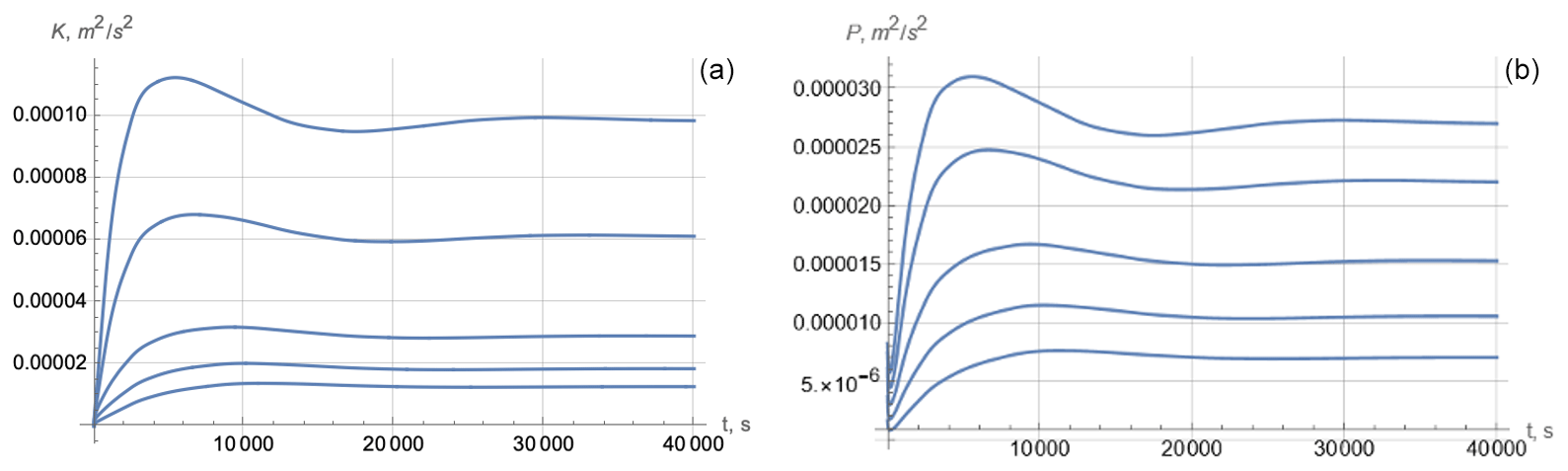
Figure 2Temporal variation of kinetic (a) and potential (b) energy for the conditions of cruise JC29. From top to bottom: , and 180 m. Here, m2 s−2.
The general equations obtained in Ostrovsky and Troitskaya (1987) (see also Gladskikh et al., 2023), are shown in the Appendix. Here they will be used for the particular case of known profiles of horizontal current shear , where 〈ux〉=V(z) is the ensemble-average horizontal velocity, and the average density is 〈ρ(z)〉=R(z). Here, z is the vertical coordinate. As a result, we have a system of two equations for the kinetic energy of turbulence K(t,z) and potential energy P(t,z) per unit volume. The latter is related to the density fluctuations :
Here, g is the gravity acceleration, R(z) is defined above, and N2(z) is the squared Brunt–Väisala frequency. Note that here the z direction is chosen downwards. Under the above conditions, the general Eq. (18) of Ostrovsky and Troitskaya (1987) and Eq. (6) of Gladskikh et al. (2023) are reduced to two equations for K:
Here, L is the outer scale of turbulence and G is the anisotropy parameter tending to 1 for strongly anisotropic turbulence with a small vertical scale compared to the horizontal scale. For details, see Ostrovsky and Troitskaya (1987). Here we consider the model of locally isotropic turbulence, for which G∼0.5. The parameter L can be taken from empirical data (Rodi, 1980) or found from the turbulence spectrum (Forryan et al., 2013; Lozovatsky et al., 2006). C and D are empirical constants. The terms and in Eq. (2) define the dissipation rates of kinetic and potential energy, respectively.
Before analyzing the full system (2), we note that some significant conclusions can be made from a reduced, local ODE system following from Eq. (2) after neglecting the last, diffusive terms in these equations:
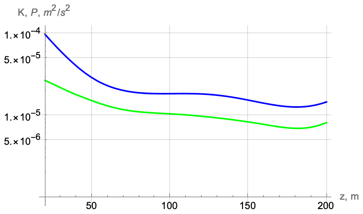
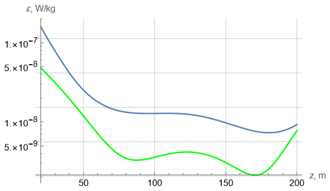
Figure 4Profiles of the turbulent kinetic energy dissipation rate for JC29. Green – interpolated data of Forryan et al. (2013). Blue – theory.
The coordinate z is now a parameter in these equations. In particular, they define a stationary distribution (a stable equilibrium point on the phase plane of variables K and P):
where is the Richardson number, and
It is noteworthy that, at Ri→∞, f has a non-zero limit (it is 1.2 for G=0.5). Hence, the turbulent energy remains finite at large Richardson numbers. General features of this solution and the turbulent Prandtl number following from it are discussed in Ostrovsky and Troitskaya (1987) and Gladskikh et al. (2023). In what follows, the applicability of these simple solutions will be verified by comparison with the solutions of the full Eq. (2). In the experiments, the dissipation rate of kinetic turbulent energy ε is commonly measured as a characteristic of turbulence. Within the semi-empirical approach, it is defined as (Kolmogorov, 1941)
It is necessary to choose the empirical constants in the above equations and in Eq. (6). There exists a broad literature discussing these values for different laboratory and on-site conditions. In the semi-empirical models they are commonly defined by scaling. We choose the outer turbulence scale based on the results of the spectral approach (Forryan et al., 2013; Galperin et al., 2007), in which the minimal wave number for the energy-carrying spectrum approximated by empirical functions is about 2 cpm. Here we take L=0.58 m. The range of the constant C is also wide in the literature. Since we are mainly interested in the quasi-equilibrium regime when the shear source is balanced with dissipation of turbulent energy, we use the data of Rodi (1980) to take . Anyway, we are mainly concerned with the order of the obtained values; indeed, in the data of Forryan et al. (2013) considered below, the spread of the data is up to an order of magnitude.
In what follows, we solve systems (2) and (3) using the Wolfram Mathematica 13 program and compare them with each other and the data of in situ measurements.

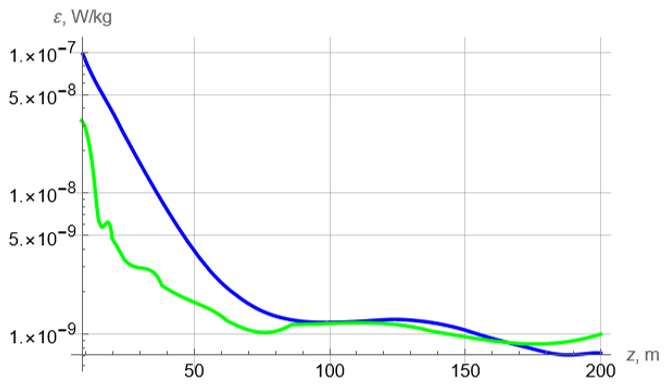
Figure 6Profiles of the turbulent kinetic energy dissipation rate for D306. Green – interpolated data of Forryan et al. (2013). Blue – theory.
As mentioned, here we apply the theory to the data of the three cruises described in Forryan et al. (2013). First, we digitized the red curves in Fig. 2 of that paper (as mentioned, there is a large dispersion of real data, but we naturally use the mean profiles). Then, using the given profiles of Vz and N2, we calculated the Richardson number as shown in Fig. 1.
Note that, for a water density of 1000 kg m−3, the static pressure (dbar) coincides with depth in meters, so that in our calculations we use the depth, neglecting small differences in density. As seen from Fig. 1, the Richardson number exceeds 1 within all ranges of the available data, and its maximum lies in the range of 10–23.
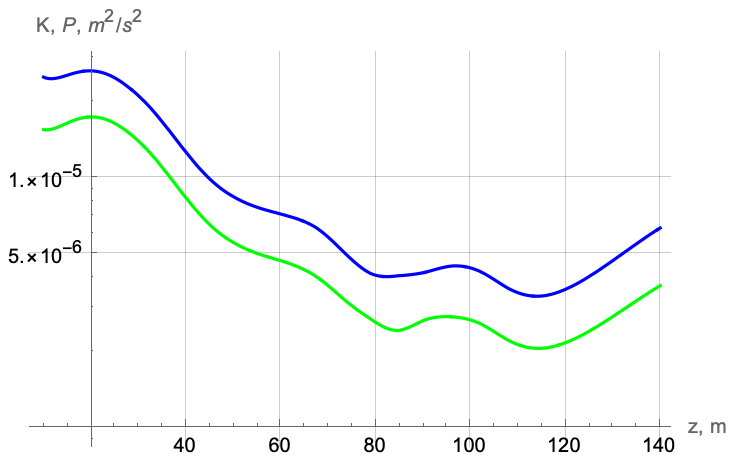

Figure 8Profiles of the turbulent kinetic energy dissipation rate for D321. Green – interpolated data of Forryan et al. (2013). Blue – theory.
3.1 Cruise JC29
Now, using the interpolation of digitized data for N2 and Vz given in Fig. 2 of Forryan et al. (2013), we solved Eq. (3) with the initial conditions and (we remind the reader that, in the local model, z is a given parameter). The values K0 and P0 varied from 10−6 to 10−5 m2 s−2 with slight changes in transient processes but with the same asymptotic values of K and P at large times. Figure 2 shows the solutions for several depths covering the range shown in Forryan et al. (2013).
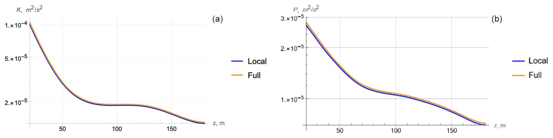
Figure 9Cruise JC29: comparison of profiles of kinetic (a) and potential (b) energies obtained from (3) (local) and (2) (full).

Figure 10Cruise D306: comparison of profiles of kinetic (a) and potential (b) energies obtained from (3) (local) and (2) (full).

Figure 11Cruise D321: comparison of profiles of kinetic (a) and potential (b) energies obtained from (3) (local) and (2) (full).
Here, the constant levels of energy are established in several hours. It is natural to use the asymptotic values for comparison with the measurement data. In the subsequent plots we use the log–lin presentation, following Forryan et al. (2013). Figure 3 shows the depth profile of the energies at large times. Note that, according to the second Eq. (4), the asymptotic values of P and K follow each other.
Using this solution, we calculate the turbulent dissipation rate (Eq. 6) and compare it with the data of Forryan et al. (2013) after digitizing both and interpolating them by smooth functions. The result is shown in Fig. 4. Here the difference between theory and measurements is mainly within a half-order. Considering the large spread of experimental data, this is a rather good agreement.
3.2 Cruise D306
To save space, for another two cruises, we show only the asymptotic profiles of the corresponding values at large times. For cruise D306, the values of kinetic and potential energies are of the same order as for cruise JC29 (Fig. 5).
Figure 6 shows the turbulence dissipation rate.
Here again, the difference between the theory and data of Forryan et al. (2013) is within a half-order.
The above results were obtained neglecting vertical turbulence diffusion. To verify this approximation, we solved the full system (2) with the same parameters and initial conditions, adding boundary conditions for fluxes of kinetic and potential energy:
They are given to be compatible with the initial conditions at initial points z0 from which the plots start in Fig. 2 of Forryan et al. (2013) and tend to zero values at the deepest points. Then, the solutions for K and P were compared with those of the local system (3). The figures below show such a comparison for the asymptotic values. In what follows, the above local solutions are shown in blue and the solutions of Eq. 2 with diffusion in orange.
In all three cases, the local and full models are practically identical. Evidently, this means the closeness of data for the dissipation rate that is a function of K. Hence, for the vertical scales of average values, vertical diffusion can be neglected, and one can use the simplified local Eq. (3).
In this paper we demonstrated that including the potential energy of turbulence (associated with density fluctuations in the presence of stratification) in the semi-empirical Reynolds-type equations of a turbulent flow allows us to explain the existence and evaluate the parameters of small-scale turbulence at large Richardson numbers. Application of these equations to the results of Forryan et al. (2013), where the measurements of profiles of the buoyancy frequency, current shear and dissipation rate of turbulent energy are shown together for three different areas of the ocean, provide not only qualitative but also reasonable quantitative agreement between the theoretical and experimental data. We have also shown that the contribution of turbulent diffusion to the level of turbulent pulsations is insignificant in the above case.
For further progress, more specific experimental data sets are desirable. Indeed, in the above calculations, we used the average data for buoyancy frequency, velocity shear, and rate of kinetic energy dissipation plotted in red in Fig. 2 of Forryan et al. (2013). However, the same figure shows significant, up to 1 order of magnitude, data scatter from each cruise, obtained in different locations and on different days. The authors do not specify the confidence intervals of the data, and no correlation between the different curves for the shear and buoyancy frequency curves is known. Still, it is possible to evaluate the maximal span of the results based on the extreme curves in each plot. For that, we digitized the leftmost and rightmost curves for the shear and buoyancy, interpolated them, and used the resulting functions to calculate the limits of the theoretical dissipation rate using Eqs. (4) and (5). For cruise 306, this is shown in Fig. 12.
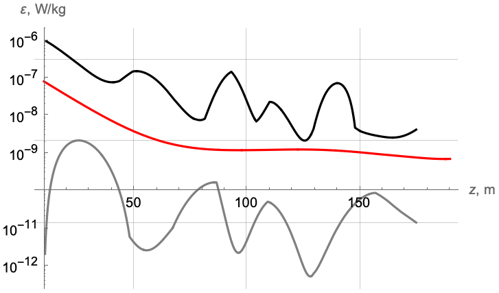
Figure 12Maximal (black) and minimal (gray) profiles of the turbulent kinetic energy dissipation rate for D306 calculated from the maximal possible scatter of data for N2 and S given in Forryan et al. (2013). Red – the average value shown in blue in 6.
Note that the data scattering for this value shown in Forryan et al. (2013) lies within the maximal theoretical limits, which implies that, knowing the real data for a specific location and time of measurement, we would reasonably predict the corresponding depth dependence for the turbulent kinetic energy dissipation rate. Similar results take place for other cruises.
Note in conclusion that the kinetic approach used in the equations used above allows us to naturally include the potential energy under consideration. Considering a large variation of empirical parameters given in different sources (Smyth et al., 2013; Liu et al., 2017; You et al., 2003), for further study it seems important to find more experimental data allowing us to apply the theory. We also plan to extend the present approach to description of time-varying turbulence in the field of internal waves (e.g., Moum et al., 2022).
Here we briefly outline the general system of equations for a turbulent stratified flow obtained in Ostrovsky and Troitskaya (1987) and developed in Soustova et al. (2020) and Gladskikh et al. (2023). Without dwelling on the details which are described in these works, here we briefly outline the main points of the model. It begins by introducing the variable probability distribution function:
where δ is the Dirac delta function and the angular parentheses denote the ensemble averaging. Using this together with the Navier–Stokes equations for u and ρ and supposing a Gaussian distribution function, the authors of Ostrovsky and Troitskaya (1987) obtained expressions for the average fluxes of turbulent energy, momentum, and mass. They are the same as in the common K−ε theory, except for the mass flux, with the form
where , and L, as above, is the outer scale of turbulence, g is the gravity acceleration, and βi are the components of the vector
which characterizes the effect of pressure fluctuations arising from random displacements of a particle in a stratified fluid.
Equation (A2) for the mass flux includes the summand , which, as shown below, leads to some significant differences from results obtained within the framework of known gradient models. The physical meaning of the additional terms in the expression mentioned above is related to the dependence of the force acting upon a random displacement of a liquid particle in a stratified medium on the shape of the liquid volume, i.e., on the ratio of the characteristic scales Lz and Lr. As shown in Ostrovsky and Troitskaya (1987), the components of the vector β have the form for a statistically homogeneous field of density fluctuations. Here, R is the anisotropy parameter:
where Lz and Lr are the vertical and horizontal scales, respectively, of the density field correlation.
As a result, one obtains the equations for the mean values of velocity, density, turbulent kinetic energy , and variance of density pulsations :
In an incompressible fluid considered here, ∇u=0. The potential energy of fluctuations is determined from the last Eq. (A8). Equation (A6) is a particular case of this system for the given average current and density stratification. In general, such effects as internal wave damping by turbulence can be included in the solution as well. On the other hand, the turbulence “breakdown” phenomenon, in which, in certain phases of the wave, the velocity shear cannot maintain a nonzero level of turbulent energy obtained using the common semi-empirical equations (Ivanov et al., 1983), does not exist here. This is also confirmed by numerical calculations using the parametrization based on the model above, given in the work (Gladskikh et al., 2023).
All the materials in the text and figures were created by the authors using standard mathematical and numerical analysis using Wolfram Mathematics software tools. Implementations of specific expressions given in the work can be provided upon request by email to the contact author.
The work did not use any external data other than those explicitly given in Forryan et al. (2013).
The concept of the article was proposed by LO. Data curation was performed by IS and DG. The formal analysis was carried out by LO and DG. The study was supervised by LO and YT. The original draft was prepared by LO, IS and DG. LO and DG worked on the review and editing.
The contact author has declared that none of the authors has any competing interests.
Publisher's note: Copernicus Publications remains neutral with regard to jurisdictional claims made in the text, published maps, institutional affiliations, or any other geographical representation in this paper. While Copernicus Publications makes every effort to include appropriate place names, the final responsibility lies with the authors.
The work was supported by RSF project no. 23-27-00002.
This research has been supported by the RSF (project no. 23-27-00002). Publisher's note: the article processing charges for this publication were not paid by a Russian or Belarusian institution.
This paper was edited by Harindra Joseph Fernando and reviewed by two anonymous referees.
Avicola, G., Moum, J., Perlin, A., and Levine, M.: Enhanced turbulence due to the superposition of internal gravity waves and a coastal upwelling jet, J. Geophys. Res., 112, C06024, https://doi.org/10.1029/2006JC003831, 2007. a
Burchard, H.: Applied Turbulence Modelling in Marine Waters, Springer, Berlin/Heidelberg, Germany, ISBN 978-3-540-45419-9, 2002. a
Burchard, H. and Bolding, K.: Comparative analysis of four second-moment turbulence closure models for the oceanic mixed layer, J. Phys. Oceanogr., 31, 1943–1968, https://doi.org/10.1175/1520-0485(2001)031<1943:CAOFSM>2.0.CO;2, 2002. a
Forryan, A., Martin, A., Srokosz, M., Popova, E., Painter, S., and Renner, A.: A new observationally motivated Richardson number based mixing parametrization for oceanic mesoscale flow, J. Geophys. Res.-Oceans, 118, 1405–1419, https://doi.org/10.1002/jgrc.20108, 2013. a, b, c, d, e, f, g, h, i, j, k, l, m, n, o, p, q, r, s, t, u, v, w, x, y
Galperin, B. and Sukoriansky, S.: QNSE theory of the anisotropic energy spectra of atmospheric and oceanic turbulence, Phys. Rev. Fluids, 5, 063803, https://doi.org/10.1103/PhysRevFluids.5.063803, 2020. a
Galperin, B., Sukoriansky, S., and Anderson, P.: On the critical Richardson number in stably stratified turbulence, Atmos. Sci. Lett., 8, 65–69, https://doi.org/10.1002/asl.153, 2007. a, b
Galperin, B., Sukoriansky, S., and Qiu, B.: Seasonal oceanic variability on meso-and submesoscales: a turbulence perspective, Ocean. Dynam., 71, 475–489, https://doi.org/10.1007/s10236-021-01444-1, 2021. a, b
Gladskikh, D., Ostrovsky, L., Troitskaya, Y., Soustova, I., and Mortikov, E.: Turbulent transport in a stratified shear flow, J. Mar. Eng. Technol., 11, 136, https://doi.org/10.3390/jmse11010136, 2023. a, b, c, d, e, f
Hostetler, S., Bates, G. T., and Giorgi, F.: Interactive coupling of a lake thermal model with a regional climate model, J. Geophys. Res., 98, 5045–5057, https://doi.org/10.1029/92JD02843, 1993. a
Ivanov, A., Ostrovsky, L., Soustova, I., and Tsimring, L.: Interaction of internal waves and turbulent in the upper layer of the ocean, Dynam. Atmos. Oceans, 7, 221–232, 1983. a, b
Kolmogorov, A.: Lokalnaja struktura turbulentnosti v neschtschimaemoi schidkosti pri otschen bolschich tschislach Reynoldsa, Dokl. AN SSSR, 30, 299–303, 1941 (in Russian). a
Liu, Z., Lian, Q., Zhang, F., Wang, L., Li, M., Bai, X., and Wang, F.: Weak thermocline mixing in the North Pacific low-latitude western boundary current system, Geophys. Res. Lett., 44, 530–539, https://doi.org/10.1002/2017GL075210, 2017. a
Ljungemyr, P., Gustafsson, N., and Omstedt, A.: Parameterization of lake thermodynamics in a high-resolution weather forecasting mode, Tellus A, 48, 608–621, 1996. a
Lozovatsky, I., Roget, E., Figueroa, M., Fernando, H. J. S., and Shapovalov, S.: Sheared turbulence in weakly stratified upper ocean, Deep-Sea Res. Pt. I, 53, 387–407, https://doi.org/10.3390/jmse11010136, 2006. a
Mackay, M.: Modeling the regional climate impact of boreal lakes, Geophys. Res. Abstr., 8, 05405, 2006. a
Mellor, G. and Yamada, T.: Development of a turbulence closure model for geophysical fluid problems, Rev. Geophys. Space Phys., 20, 851–875, https://doi.org/10.1029/RG020i004p00851, 1982. a
Monin, A. and Ozmidov, R.: Ocean Turbulence, Gidrometeoizdat, Leningrad, Russia, 1981 (in Russian). a
Monin, A. and Yaglom, A.: Statisticheskaya gidromekhanika, chap. 1, Nauka, Moscow, 1965 (in Russian). a
Moum, J., Hughes, K., Shroyer, E., Smyth, W., Cherian, D., Warner, S., Bourlès, B., Brandt, P., and Dengler, M.: Deep cycle turbulence in Atlantic and Pacific cold tongues, Geophys. Res. Lett., 49, e2021GL097345, https://doi.org/10.1029/2021GL097345, 2022. a
Ostrovsky, L. and Soustova, I.: Upper mixed layer of the ocean as a sink of internal wave energy, Okeanologia, 19, 973–981, 1969 (in Russian). a
Ostrovsky, L. and Troitskaya, Y.: Model of turbulent transfer and the dynamics of turbulence in a stratified shear flux, Izv. Akad. Nauk SSSR, Fiz. Atmos. Okeana, 3, 101–104, 1987. a, b, c, d, e, f, g, h, i, j
Rodi, W.: Prediction Methods for Turbulent Flows, edited by: Kollman, W., Hemisphere, New York, 1980, 259–350, ISBN 978-0070352599, 1980. a, b
Smyth, W., Moum, J., Li, L., and Thorpe, S.: Diurnal shear instability, the descent of the surface shear layer, and the deep cycle of equatorial turbulence, J. Phys. Oceanogr., 43, 2432–2455, https://doi.org/10.1175/JPO-D-13-089.1, 2013. a, b
Soustova, I., Troitskaya, Y., Gladskikh, D., Mortikov, E., and Sergeev, D.: A simple description of the turbulent transport in a stratified shear flow as applied to the description of thermohydrodynamics of inland water bodies, Izv. Atmos. Ocean. Phys., 56, 603–612, https://doi.org/10.1134/S0001433820060109, 2020. a, b, c
Strang, E. and Fernando, H.: Vertical mixing and transports through a stratified shear layer, J. Phys. Oceanogr., 31, 2026–2048, https://doi.org/10.1175/1520-0485(2001)031<2026:VMATTA>2.0.CO;2, 2001. a
Stretch, D., Rot, J., Nomura, K., and Venayagamoorthy, S.: Transient mixing events in stably stratified turbulence, in: Proceedings of the 14th Australasian Fluid Mechanics Conference, Adelaide, Australia, 10–14 December 2001, 625–628, 2001. a
Sukoriansky, S., Galperin, B., and Staroselsky, I.: Cross-term and ε-expansion in RNG theory of turbulence, Fluid Dyn. Res., 33, 319, 10.1016/j.fluiddyn.2003.08.001, 2003. a
Sukoriansky, S., Galperin, B., and Perov, V.: Application of a new spectral theory of stably stratified turbulence to atmospheric boundary layer over sea ice, Bound.-Lay. Meteorol., 117, 231–257, https://doi.org/10.1007/s10546-004-6848-4, 2005a. a
Sukoriansky, S., Galperin, B., and Staroselsky, I.: A quasi-normal scale elimination model of turbulent flows with stable stratification, Phys. Fluids, 17, 085107, https://doi.org/10.1063/1.2009010, 2005b. a
Tsuang, B.-J., Tu, C.-J., and Arpe, K.: Lake parameterization for climate models, Tech. Rep. 316, Max Planck Institute for Meteorology, ISSN 0937-1060, 2001. a
You, Y., Suginohara, N., Fukasawa, M., Yoritaka, H., Mizuno, K., Kashino, Y., and Hartoyo, D.: Transport of North Pacific Intermediate Water across Japanese WOCE sections, J. Geophys. Res., 108, 3196, https://doi.org/10.1029/2002JC001662, 2003. a
Zilitinkevich, S., Elperin, T., Kleeorin, N., and Rogachevskii, I.: Energy-and flux-budget (EFB) turbulence closure models for stably-stratified flows. Part I: Steady-state, homogeneous regimes, Bound.-Lay. Meteorol., 125, 167–191, https://doi.org/10.1007/s10546-007-9189-2, 2007. a
Zilitinkevich, S., Elperin, T., Kleeorin, N., Rogachevskii, I., and Esau, I.: A hierarchy of Energy and Flux-Budget (EFB) turbulence closure models for stably stratified geophysical flow, Bound.-Lay. Meteorol., 146, 341–373, https://doi.org/10.1007/s10546-012-9768-8, 2013. a
- Abstract
- Introduction
- Basic equations
- Application of the local model
- Comparison with the full system
- Discussion and conclusions
- Appendix A: Dynamical equations for a turbulent stratified flow
- Code availability
- Data availability
- Author contributions
- Competing interests
- Disclaimer
- Acknowledgements
- Financial support
- Review statement
- References