the Creative Commons Attribution 4.0 License.
the Creative Commons Attribution 4.0 License.
 | 23 Apr 2024
Transformation of internal solitary waves at the edge of ice cover
Kateryna Terletska
Elena Tobisch
Internal wave-driven mixing is an important factor in the balance of heat and salt fluxes in the polar regions of the ocean. Transformation of internal waves at the edge of the ice cover can enhance the mixing and melting of ice in the Arctic Ocean and Antarctica. In the polar oceans, internal solitary waves (ISWs) are generated by various sources, including tidal currents over bottom topography, the interaction of ice keels with tides, time-varying winds, vortices, and lee waves. In this study, a numerical investigation of the transformation of ISWs propagating from open water in the stratified sea under the edge of the ice cover is carried out to compare the depression ISW transformation and loss of energy on smooth ice surfaces, including those on the ice shelf and glacier outlets, with the processes beneath the ridged underside of the ice. They were carried out using a non-hydrostatic model that is based on the Reynolds-averaged Navier–Stokes equations in the Boussinesq approximation for a continuously stratified fluid. The Smagorinsky turbulence model extended for stratified fluid was used to describe the small-scale turbulent mixing explicitly. Two series of numerical experiments were carried out in an idealized 2D setup. The first series aimed to study the processes of the ISWs of depression transformation under an ice cover of constant submerged ice thickness. Energy loss was estimated based on a budget of depth-integrated pseudoenergy before and after the wave transformation. The transformation of ISWs of depressions is controlled by the blocking parameter β, which is the ratio of the minimum thickness of the upper layer under the ice cover to the incident wave amplitude. The energy loss was relatively small for large positive and large negative values of β. The maximal value of energy loss was about 38 %, and it was reached at β≈0 for ISWs. In the second series of experiments, a number of keels were located on the underside of the constant-thickness ice layer. The ISW transformation under ridged ice also depends on the blocking parameter β. For large keels (β<0), more than 40 % of energy is lost on the first keel, while for relatively small keels (β>0.3), the losses on the first keel are less than 6 %. Energy losses due to all keels depend on the distance between them, which is characterized by the parameter μ, i.e. the ratio of keel depth to the distance between keels. In turn, for a finite length of the ice layer, the distance between keels depends on the keel quantity.
- Article
(3528 KB) - Full-text XML
- BibTeX
- EndNote


Internal wave-driven mixing is an important factor in the balance of heat and salt fluxes in the polar regions of the ocean (Guthrie et al., 2013). In these areas, internal gravity waves are generated by various sources, including tidal currents over the bottom topography (Urbancic et al., 2022), time-varying winds (Rainville and Woodgate, 2009), vortices (Johannessen et al., 2019), and lee waves (Vlasenko et al., 2003). Another source of energy for internal waves in the near-surface pycnocline can be interaction of ice keels with tides (Zhang et al., 2022a). These waves, in the form of internal solitary waves (ISWs), often propagate along the pycnocline in a stratified ocean under ice cover. The interaction between internal waves and ice cover is complex and depends on both the characteristics of the ice and the characteristics of internal waves (Carr et al., 2019). The transformation of an ISW under an ice keel can cause the advection of water below the ice layer due to wave motion, whereas ISW shear and convective instabilities result in turbulent mixing. The heat advection and turbulent flux will both contribute to the vertical heat flux and consequently the change in temperature under the sea ice and the increase in melting (Zhang et al., 2022b). An increased level of dissipation of the energy of internal waves propagating from the open water should be expected at the edge of the ice cover, which can represent the edge of an ice shelf or pack ice. In turn, the relief of the underside of the ice and, in particular, the presence of ice keels can essentially affect ISW transformation, breaking, and energy dissipation. These aspects of the complicated problem of the interaction of internal waves and ice cover have not yet been investigated due to severe conditions for field observations in the polar regions of the ocean.
The problem of the transformation of a depression ISW under smooth ice cover is mathematically close to the problem of the transformation of an elevation IWS over a bottom step of constant height which has been considered analytically (Grimshaw et al., 2008) and numerically using a non-hydrostatic model (Maderich et al., 2009; Talipova et al., 2013). It was found that the transformation of an ISW over the step in a two-layer fluid depends on the ratio of the thickness of the lower layer over the step to the ISW amplitude. The transformation of the elevation ISW over a single obstacle (ridge) on the bottom has been studied in the laboratory (Wessels and Hutter, 1996; Chen, 2007; Du et al., 2021) and numerically (Vlasenko and Hutter, 2001; Xu et al., 2016). Wave breaking on the lee side of the ridge was accompanied by the generation of second-mode ISWs. The propagation of an elevation ISW over a corrugated bed (Carr et al., 2010) was accompanied by shear instability in the form of billows. ISWs propagating from open water to ice were studied in the laboratory by Carr et al. (2019) for grease, level, and nilas ice. The experiments showed that the dissipation of turbulent kinetic energy under the ice is comparable to that of the ISW in the water column. The disintegration of an ISW of a depression under a single ice keel was simulated by Zhang et al. (2022b). It was concluded that the corresponding turbulent mixing can enhance the melting of ice keels.
In this study, a numerical investigation of the transformation of an ISW propagating from ice-free water in the stratified sea under the edge of the ice cover is carried out to compare the depression ISW transformation and loss of energy on smooth ice surfaces, including those on the ice shelf, with the processes beneath the ridged underside of the ice. The rest of the paper is organized as follows. The formulation of the problem, the model setup, and the relevant numerical tools are given in Sect. 2. Section 3.1 presents the simulation results for smooth ice cover, whereas the results of the simulation of ridged ice cover are considered in Sect. 3.2. The results of the simulations are summarized and discussed in Sect. 4.
The numerical simulations were carried out using a non-hydrostatic model (Maderich et al., 2012). The numerical model used here is based on the Reynolds-averaged Navier–Stokes equations in the Boussinesq approximation for a continuously stratified fluid. The Smagorinsky turbulence model extended for stratified fluid (Siegel and Domaradzki, 1994) was used to explicitly describe the small-scale turbulent mixing in the ocean-scale ISWs. Two series of numerical experiments were carried out in an idealized 2D setup. The first series aimed to study processes of the ISWs of depression transformation under ice cover of constant submerged ice thickness (draft) hice (Fig. 1a). The second series was carried out to simulate the effect of ridged ice on ISWs of depression propagation in a similar two-layer stratification (Fig. 1b). A computational tank of constant depth H=200 m and length L=10 000 m was used. It was assumed that the ice layer of length Lice=5000 m is rigid and does not interact with the ISWs. The coordinate x is directed along the computational domain, and z is directed vertically upward. Idealized stratification of the vertical distribution of potential density is considered in the form
where h1 is the thickness of the upper layer of water in the absence of the ice cover, is the thickness of the lower layer, and . As shown by Maderich et al. (2010) and Talipova et al. (2013), the transformation of both elevation and depression ISWs is controlled by the blocking parameter β, which is the ratio of the height of the minimum thickness of the upper layer under the ice cover h1+ to the incident wave amplitude ai:
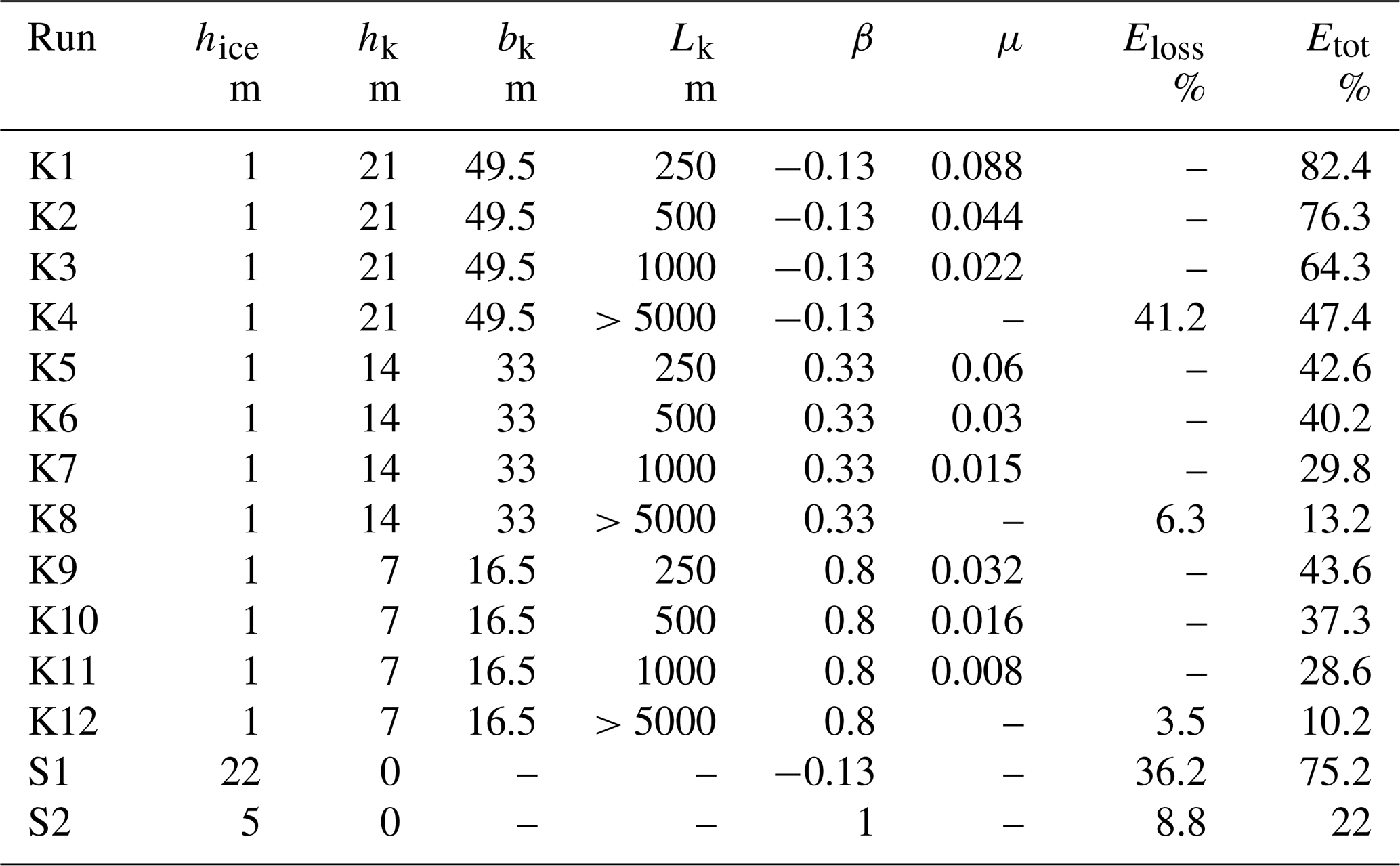
where β is positive in the case , (h1>hice) and negative for , (h1<hice). In the first series, submerged ice thickness hice was constant along the computational tank varying in different numerical experiments from 0.5 to 40 m (Table 1). In the second series of experiments, several keels were placed under the ice layer of constant thickness hice (Fig. 1b). The ice keel shape was approximated by the Versoria function (Skyllingstad et al., 2003) as
where hk is the maximal keel penetration, bk is a parameter governing the determination of the keel width, and is the horizontal distance from the centre of the keel placed at xk. The keel form was similar, i.e. is constant. Following Zhang et al. (2022b), we define keel width as the horizontal width of the consolidated ice zone at a depth of 4 m below the bottom of the ice (Marchenko, 2008). Typical values of hk are 3–28 m (Strub–Klein and Sudom, 2012), reaching 45 m (Leppäranta, 2007), whereas typical keel widths vary in the range 3–200 m (Strub–Klein and Sudom, 2012). In the ocean, the ratio of the maximum height of the keel hk to the distance between the keels Lk varies from for heavily ridged ice to for moderately ridged ice (Lu et al., 2011). For this idealized case study, the vertical distribution of the potential density anomaly mimics the summer profile of potential density over the Yermak Plateau (Randelhoff et al., 2017) in the Arctic Ocean (Eq. 1), where h1=20 m, △h=10 m, σθ1=25.4 kg m−3, and σθ2=27.7 kg m−3. As seen in Fig. 2, the summer profile of density does not have a well-mixed surface layer due to the stratification caused by ice melting. Free-slip boundary conditions were used at all the boundaries, except along the ice–water boundary. The Neumann-type boundary condition for the non-hydrostatic pressure component was used at the solid boundaries. At the free surface and open boundaries, this component was set to zero (Maderich et al., 2012). At the corner of the underwater step, this condition is violated. However, numerical experiments for different resolutions have shown that this problem does not occur at simulated fields of velocity and density. Ice–ocean tangential stress is parameterized using the quadratic bulk formula with a drag coefficient CD. The value of CD under ice varies in the range 10−3–10−2 (Lu et al., 2011). A no-flux condition was also used at all the boundaries. The model was initialized using the iterative solution of the Dubreil–Jacotin–Long (DJL) equation (Dubreil-Jacotin, 1932), with the initial guess obtained from a weakly non-linear theory. The DJLES spectral solver from the MATLAB package (https://github.com/mdunphy/DJLES/, last access: 28 February 2024) was used to generate ISWs of depression. To get around the difficulties associated with the numerical solution of the non-hydrostatic model equations in the presence of an ice layer, we considered the setting mirrored for the upper surface of the ocean, in which the ice layer was replaced with a step on the bottom. Then the vertical profile (Eq. 1) was replaced with the distribution
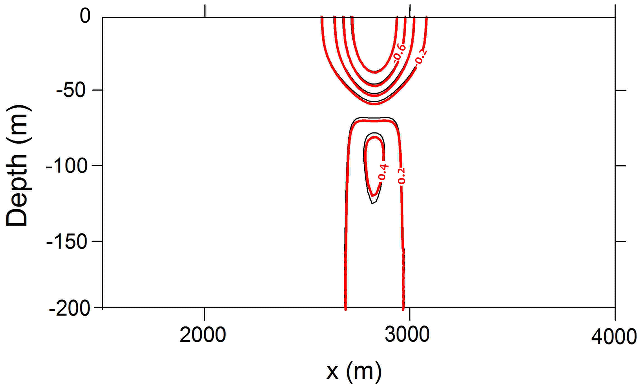
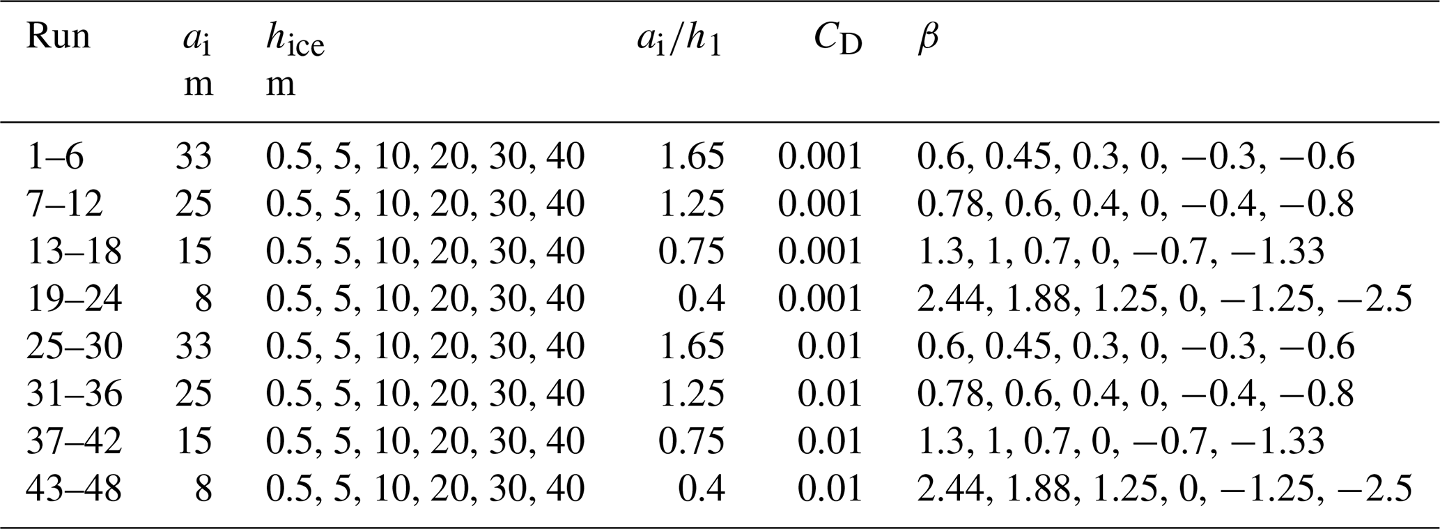
where σθ1=27.7 kg m−3 and σθ2=25.4 kg m−3. The initial ISW of the depression was changed to an ISW of elevation. This approach is accurate when we consider the problem with rigid-lid approximation at the free surface. However, the numerical model is a free-surface model, which leads to bottom fluctuations outside the step in the computational flume. Therefore, we conducted tests with ISWs of the same amplitude propagating as an ISW of depression and as an ISW of elevation in stratifications (1) and (4). The tests aimed to estimate the effect of the free surface on the wave characteristics for free-slip boundary conditions. These results demonstrate a weak effect of the free surface on ISW dynamics in the considered cases, which made it possible in this problem to replace the conditions on the free surface with conditions on the rigid lid. The results of the comparison for horizontal velocity taking into account the mirror reflection of the vertical coordinate in Fig. 3 showed that the difference in the velocity between the two configurations of the model does not exceed 1 %. Note that, in laboratory experiments (Carr et al., 2008; Luzzatto-Fegiz and Helfrich, 2014), the influence of a free surface on the stability of waves with a trapped core was shown. This effect has been interpreted as the influence of surfactants, which are essential in laboratory-scale processes. However, these Marangoni effects have a negligible impact on the interior of full-scale oceanic waves (Luzzatto-Fegiz and Helfrich, 2014). In the first series of experiments, 48 runs were performed using the generalized vertical system of coordinates (Maderich et al., 2012). The vertical and horizontal grid resolution was 400×3000. The quasi-z-level coordinate system (Maderich et al., 2012) was used to describe this step-like ice layer. These runs cover a range of incident ISWs with moderate, ai=8 m, and large, ai=33 m, amplitudes (Table 1). The incident ISW amplitude is defined as the maximum displacement of the undisturbed isopycnals. The wavelength λ0.5 is estimated as the half-width at the depth where the amplitude of the wave is reduced by half. Two cases with different drag coefficients (CD=0.001 and CD=0.01) were considered to investigate the influence of ice roughness on ISW transformation and energy loss. A wide range of ice cover drafts hice from 0.5 to 40 m was used to investigate processes under ice cover from first-year ice to the ice shelf front. In the second series of experiments (see Table 2), 12 runs (K1–K12) were performed using a sigma system of coordinates, which allowed flow around the keel to be described accurately. The vertical and horizontal grid resolution was also 400×3000. The density stratification in this series was the same as in the first series. The ISW amplitude was ai=15 m, the wavelength λ0.5=320 m, and the drag coefficient CD=0.001. The ice draft was 1 m, which mimics 1-year ice. The keel's maximal penetration hk varied from 7 to 21 m, and the width of the keel varied from 67 to 200 m at a depth of 4 m. To take into account the geometric characteristics of the keels and their frequency, we introduce the parameter μ, which is the ratio of the sum of submerged ice thickness and maximal keel penetration to the distance between keels:
In turn, for a finite length of the ice layer Lice, the distance between keels depends on keel number n as . In the second series, μ varies in experiments K1–K3 from 0.008 to 0.088 (Table 2). To directly compare with the step case, calculations were made for step (S1) with the same draft as the height of the keel in the K1–K4 experiments. In another experiment (S2), the step draft was chosen to be equal to the average draft in experiment K2.
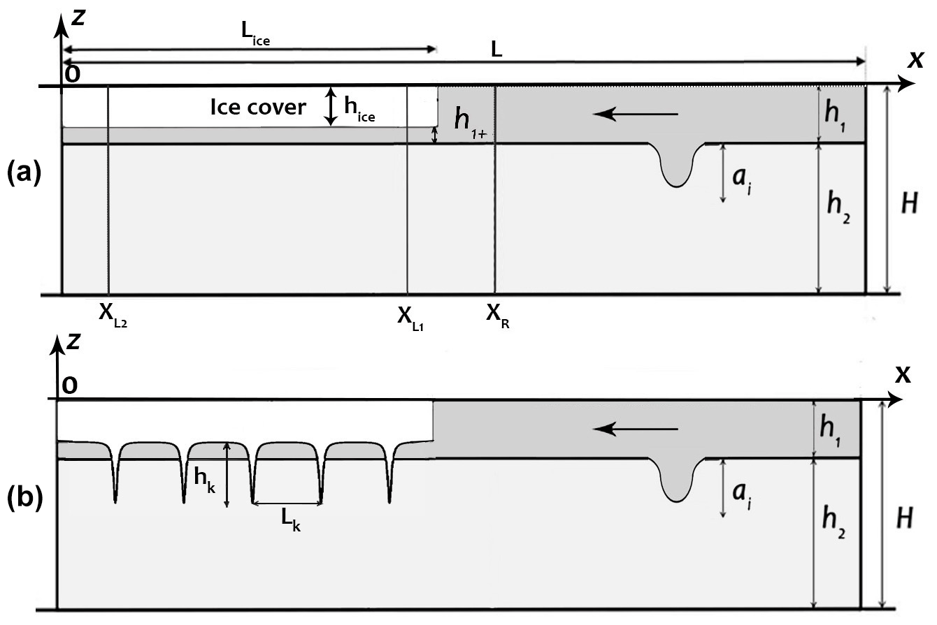
Figure 1Sketch of the numerical configuration for simulation of ISW transformation under the ice. (a) Smooth ice cover. (b) Ridged ice.
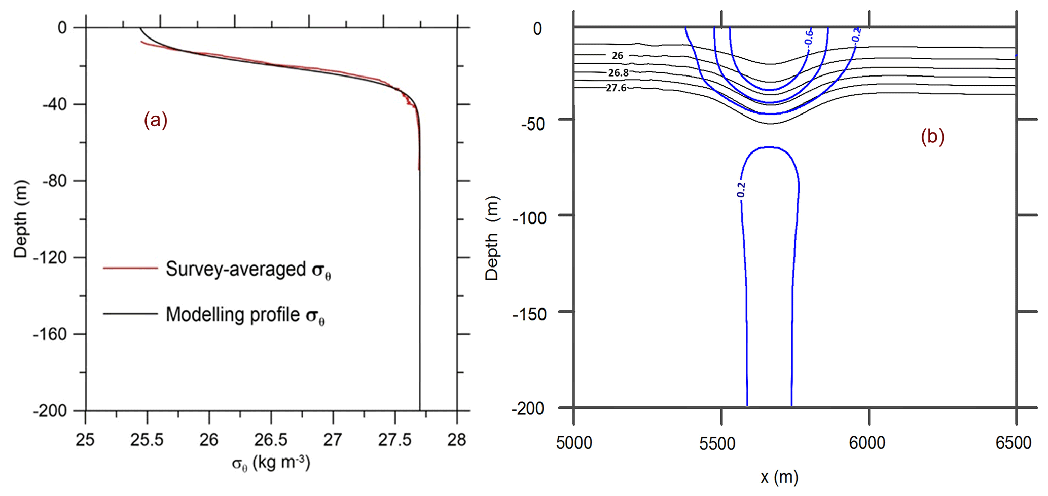
Figure 2The comparison of the background stratification in the computational tank (Eq. 1) with the survey-averaged profile of the anomaly of potential density σθ (Randelhoff et al., 2017) (a). The vertical cross section of the potential density and horizontal velocity fields in the incident ISW of amplitude 15 m (b).
3.1 First series of experiments
The results of the first series of experiments for the transformation of a depression ISW for an incident wave at the ice were given for a wide range of ice drafts, incident wave amplitudes, and drag coefficients (Table 1). The snapshots of the density field for an incident ISW of amplitude ai=15 m passing under the ice cover are shown in Fig. 4 for different β. Transformation under thin ice (hice=0.5 m) with β=1.3 occurs without any instability and essential disturbances. For increased ice draft β=0.7 (hice=10 m), the incident wave changes its form and amplitude as it passes under the ice. The amplitudes of reflected and transmitted waves were well predicted by the theoretical model (Grimshaw et al., 2008). For β=0 (hice=20 m), the transmitted wave has a smaller amplitude, and more energy is transferred to the reflected wave at the ice edge. Waves under the ice transform into strongly non-linear boluses, and more energy goes to the reflected waves when the draft of the ice is equal to the depth of the upper layer (β=0). The bolus under the ice becomes smaller, and reflected waves form as a result of the strong interaction with the ice front at (hice=30 m). An important characteristic of the ISW–ice interaction is the loss of kinetic and available potential energy during the ISW transformation. Energy transformation due to mixing leads to the transfer of energy to background potential energy and energy dissipation. Energy loss was estimated based on a budget of depth-integrated pseudoenergy before and after the wave transformation following Lamb (2007) and Maderich et al. (2010). The characteristics of the incoming and reflected waves were recorded in the cross sections XR (Fig. 1a), which are located near the ice edge, and in two cross sections: XL1 placed at a distance of 500 m from the ice edge and XL2 placed at a distance of 4500 m from the ice edge (Fig. 1a). The energy loss ΔEloss in the cross section xL1 characterizes energy transformations in the vicinity of the ice edge, whereas energy losses ΔEvisc take into account the dissipation of energy due to the underside ice friction effects. The total energy of the incident, reflected, and transmitted waves was calculated using the depth-integrated pseudoenergy flux F(x,t) to find the balance of the total energy:
where p is the pressure disturbance due to the passing wave, U is the horizontal velocity, and EPSE is the pseudoenergy density, which is the sum of the kinetic energy density Ek and the available potential density Ea (part of the potential energy available for conversion into kinetic energy). For the calculation of Ea, we used a reference density profile that was obtained by adiabatic rearranging of the density field. The volume integration of these flows outside the mixing zone allows us to estimate the energy of the incoming PSEin, reflected PSEref, and ISWs transmitted under ice in cross sections XL1, XL2 (see Fig. 1a), PSEtr1, and PSEtr2 respectively:
where t2–t1 is the interval of time when the incoming wave passes the cross section XR, and t3–t2 is the interval of time when transmitted and reflected waves pass the cross sections XL1 and XR respectively. Time interval t5–t4 corresponding to the transmitted wave passes the cross section XL2. The normalized energy losses ΔEloss, ΔEvisc, and ΔEtot are given by
The energy loss as a result of ISW transformation under ice ΔEloss at interval XR–XL1 versus the blocking parameter β is shown in Fig. 5a. This loss was relatively small for large positive and large negative values of β. The maximal value of energy loss was about 38 %, and it was reached at β≈0. The character of energy losses and the relationship between transmitted and reflected ISW energy allows us to distinguish between different regimes for ISW interaction under ice cover: the weak interaction (I), moderate interaction (II), strong interaction (III), and reflection regime (IV). The weak interaction (I) is when the ISW transforms under ice cover without any instability; the energy losses are mainly due to viscous dissipation. It corresponds to values β>0.5. The energy losses at cross sections XR–XL1 are about 10 %. The amplitudes and numbers of reflected and transmitted waves are well predicted by the theoretical model of Grimshaw et al. (2008). Moderate interaction (II) occurs when the waves become unstable under ice cover, resulting in energy losses due to the turbulent mixing varying from 10 % to 20 %. The strong interaction (III) of the ISW with the ice is the regime when the flow under the ice is supercritical. This regime is identified by the condition that the maximal composite Froude number Frmax at the step cross section is greater than 1, where Fr is defined as
where U1 and U2 are the layer-averaged velocities in each layer, , where g is the gravity acceleration, Δρ and ρ0 are the density difference between the upper and lower layers and the undisturbed density of the fluid respectively. Supercritical flow Frmax=1 with β=0 resulted in bolus formation and intensive mixing, which reached about 40 %. The reflection regime (IV) is when the height of the ice floe is large enough to result in full reflection of the ISW. The energy losses are again small (△Eloss less than 10 %–15 %). In this regime, energy losses depend on the wave amplitude; small and moderate incident waves reflect without turbulent mixing. This dependence of ΔEloss on β is comparable to values for a bottom step (Talipova et al., 2013) obtained using direct simulation by the Navier–Stokes equations (Fig. 5a). The differences in values of the energy losses from Talipova et al. (2013) and from the present investigation can be explained by the fact that the field-scale problem was studied in this work using the Reynolds-averaged equations, while in Talipova et al. (2013) the propagation of ISWs in a laboratory-scale computational domain was studied using the Navier–Stokes equations. The eddy viscosity and diffusivity calculated from the turbulence model (Siegel and Domaradzki, 1994) vary in space and time, with characteristic values of 10−4–10−3 m2 s−1. The difference between the energy losses in the cross sections XL2 and XL1 characterizes their losses due to friction effects. This difference is shown in Fig. 5b as a function of β. This shows that the contribution of friction is 15 %–20 % of the energy of the incident wave. The simulations showed a weak dependence of energy loss on the friction parameter CD (Fig. 5b).
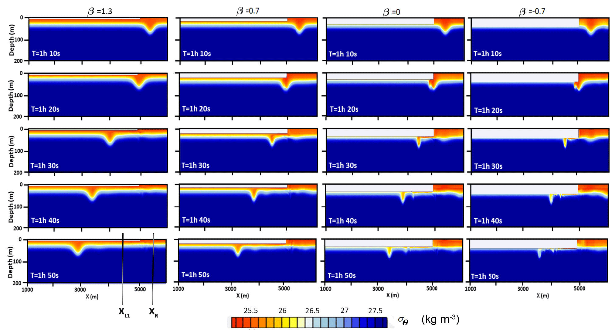
Figure 4The snapshots of the density field for an incident ISW with amplitude 15 m passing under the ice cover with a different draft. The integration region for the energetic calculations between XL1 and XR is shown.
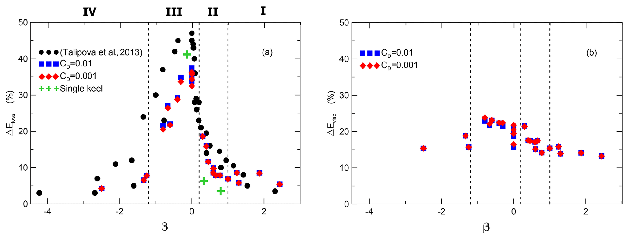
Figure 5(a) The ISW energy loss ΔEloss under the ice cover versus the blocking parameter β for various amplitudes of an incident wave (b) ΔEvisc that take into account the dissipation of energy due to the underside ice friction effects versus the blocking parameter β.
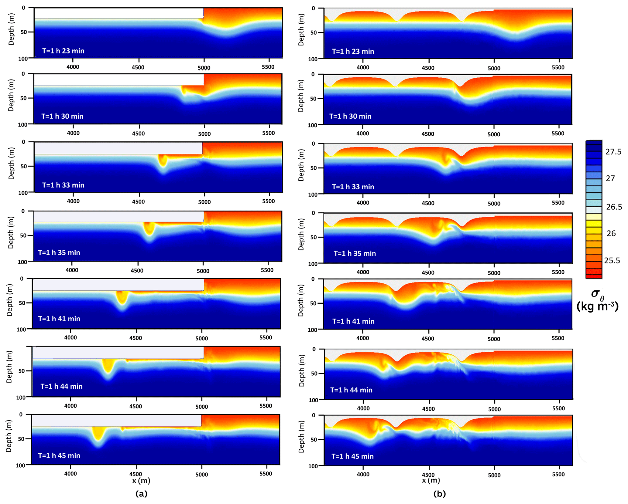
Figure 6(a) The transformation of ISWs of depression under a smooth ice layer (Run S1). (b) The transformation of ISWs of depression under a ridged ice layer (Run K2).
3.2 Second series of experiments
The results of the second series of experiments for the transformation of depression ISWs under ridged ice for different ice keel heights and distances between keels (Table 2) are discussed in this section. Similarly to Eq. (2), we can introduce the blocking parameter for a single keel in the form
The snapshots of the density field for an incident ISW passing under the layer of constant draft (Run S1 from Table 2) are compared in Fig. 6 with the results for a wave passing under ridged ice (Run K2). In Run S1 the ISW amplitude is comparable to the draft of ice and the thickness of the upper layer h1+; therefore, the interaction was strong. Initially (time interval T=1 h 30 min–1 h 35 min), the wave propagated under the ice as a bolus (Fig. 6a). This process is accompanied by intensive mixing. The bolus gradually loses mass. Estimates of energy loss at a distance of 500 m from the ice front Eloss in Run S1 (Table 2) showed that 36.2 % of the energy was lost to mixing and dissipation, whereas loss of energy at the full length of the ice cover (5000 m) was twice as much (Etot=75.2 %). The processes of ISW disintegration and mixing for ridged ice differ essentially from the case of the ice layer of the constant draft. The snapshots of the density field for the ISW passing under the ridged ice (Run K2) are shown in Fig. 6b. As seen in the figure, the flow accelerates on the rear side of the keel (T=1 h 30 min; Frmax reaches the value 1) entraining denser water from the underlying layers. The resulting vortex is accompanied by intense mixing (T=1 h 33 min–1 h 45 min). The process of transformation of this wave with a slightly smaller amplitude is repeated on subsequent keels. As a result of passing through the first keel, the wave loses about 41 % of the incident wave energy. Energy losses due to all the keels depend on the distance Lk between them, which in turn depend on the keel quantity. When , Etot changes from 47.4 % for a single keel to 82.4 % for Lk=250 m. This means that energy losses on the first keel account for about half of all the losses. For Lk=1000 m, the energy loss due to all the keels was 64.3 %. As β increases to 0.8, the contribution of the first keel decreases to 3.5 %. In the limiting case of the interaction of an ISW with a single keel (Zhang et al., 2022b), the maximum energy dissipation was about 25 %, which is somewhat less than in our calculations, but we need to keep in mind the differences in the calculation parameters and turbulence parameterization. Zhang et al. (2022b) used constant eddy coefficients, whereas in our study the turbulence model was used with eddy coefficients varying in space and time. To characterize the dependence of ΔEtot on keel height and distance between keels, we introduced parameter μ (Eq. 5). As seen in Fig. 7, this dependence can be approximated by logarithmic curves , where , , and . The energy loss ΔEtot increases with the decrease in distance between keels or an increase in keel height. The level of ΔEtot is highest for β values near zero. As seen in Fig. 5a, this range of β corresponds to the regime of strong interaction (III). Energy loss in this regime is maximal, both in the case of the ridged underside of the ice and in the case of smooth ice surfaces with the same parameter β. When β values increase, the dependence of energy loss on the μ and distance between the keels decreases. β=0.8 is on the boundary between regimes (II) and (I) (moderate and weak), and the distance between the keels is no longer significant.
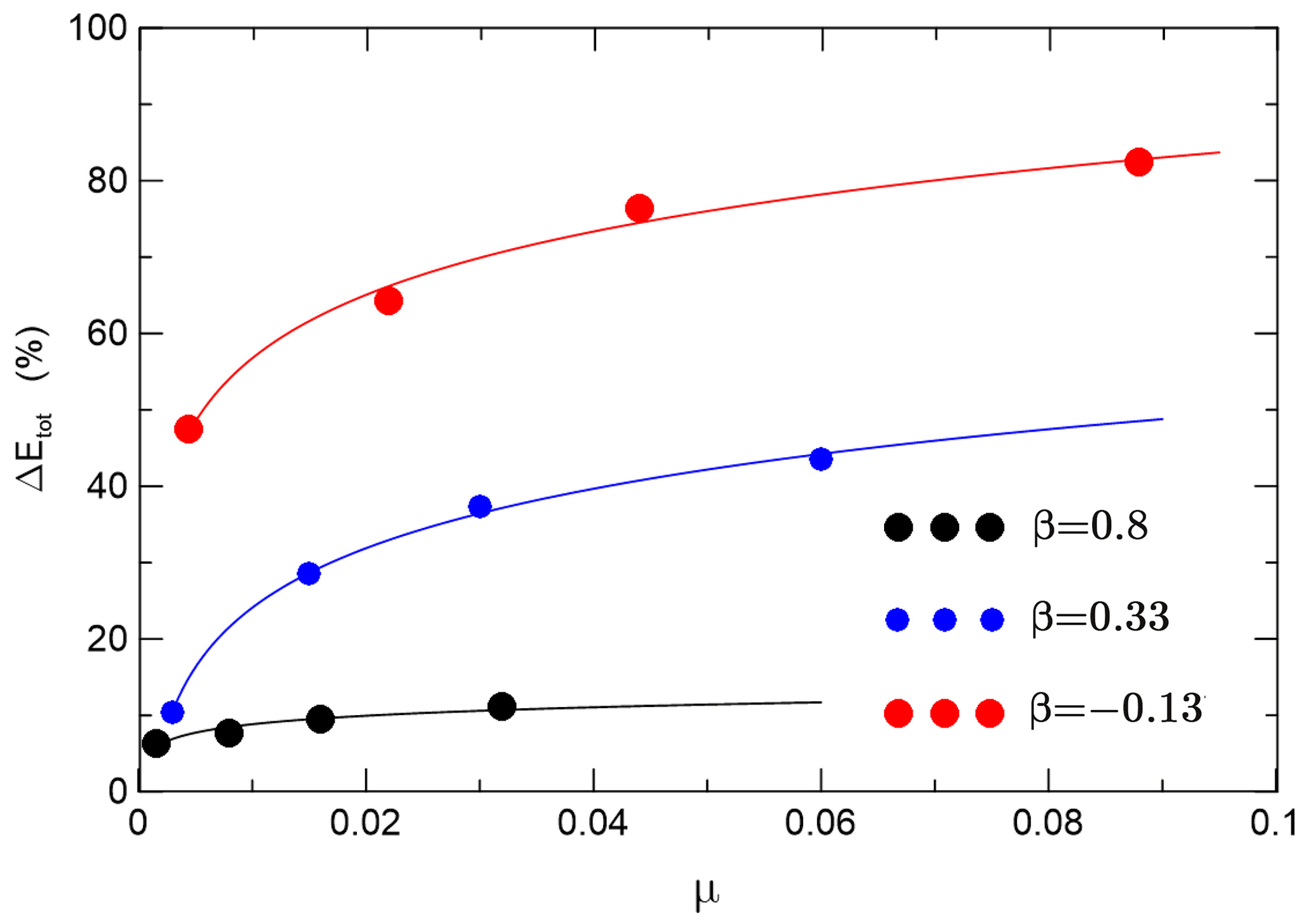
Figure 7The ISW energy loss △Eloss under the ice cover versus parameter μ. The logarithmic curves approximate calculated dependencies.
In another limiting case, an ISW of elevation propagates over a corrugated bottom when the bottom element length was much lower than the ISW wavelength (Carr et al., 2010). A comparison with an ISW propagated under an ensemble of ice keels of horizontal scales greater than the ISW length was not straightforward. In addition, Reynolds equations with turbulent closure describe real-scale processes in the ocean, in contrast to laboratory scales in Carr et al. (2010). Unlike Carr et al. (2010), we cannot describe in detail the instant spatial–temporal dynamics of high shear layers near the ice. However, Fig. 6b shows wave-induced currents over the keels, their interaction with the apex of the keels, and a sequence of lee vortices formed as a result of such interaction (see Fig. 6b: T=1 h 35 min, T=1 h 41 min). Similarly to Carr et al. (2010), the vortices developed after the main wave passed over the keel (see Fig. 6b: T=1 h 44 min, T=1 h 45 min), resulting in deformation of the overlying pycnocline and, in some instances, significant vertical mixing.
In this study, a numerical investigation of the transformation of ISWs propagating from open water in a stratified sea into an ice-covered region is carried out. We compared the transformation and energy loss of depression ISWs under smooth ice surfaces, with the processes beneath ridged ice. It was shown that the transformation of depression ISWs under smooth ice cover is controlled by the blocking parameter β. Several regimes of ISW transformation at the ice–open water boundary were identified: (I) the weak interaction when the ISW transforms under ice cover without any instability; the energy losses are caused mainly by viscous dissipation. It corresponds to values β>0.5. (II) Moderate interaction, which occurs when the waves become unstable under ice cover, results in energy losses due to the turbulent mixing varying from 10 % to 20 %. (III) Strong interaction of ISWs with the ice (β≃0) is the regime when the flow under the ice is supercritical and the values of energy loss are about 38 %. The reflection regime (IV) is when the depth of the ice cover is large enough to result in full reflection of the ISW. The ice's roughness has relatively little effect on energy conversions under ice cover.
The ISW transformation under ridged ice also depends on the blocking parameter β. For large keels (β<0), more than 40 % of the energy is lost on the first keel, while for relatively small keels (β>0.3), the losses on the first keel are less than 6 %. The energy losses in the flow around the ridges can be of the same order as for the ice cover, in which the draft is commensurate with the amplitude of the keels. Energy losses due to all the keels depend on the distance between them, which in turn depends on a keel quantity. These losses are characterized by the parameter μ, which is the ratio of the keel depth to the distance between the keels.
The energy loss processes of ISWs under ice deserve more in-depth studies to bridge ISW mixing and the heat balance of polar oceans (Pinkel, 2005). The next step could be an explicit representation of heat and salt fluxes between the ice cover due to the ISW interaction with the ridged ice, e.g. following the flux parametrization by McPhee et al. (1987).
Code and data are available from https://doi.org/10.5281/zenodo.10984509 (Maderich and Terletska, 2024).
VM designed the study, contributed to the visualization of the results, and wrote the manuscript with support from all the authors. KT contributed to the method development, simulation, data processing, and manuscript writing. ET contributed to the interpretation of the results and manuscript editing. All the authors contributed to the article and approved the submitted version.
The contact author has declared that none of the authors has any competing interests.
Publisher's note: Copernicus Publications remains neutral with regard to jurisdictional claims made in the text, published maps, institutional affiliations, or any other geographical representation in this paper. While Copernicus Publications makes every effort to include appropriate place names, the final responsibility lies with the authors.
This article is part of the special issue “Turbulence, wave–current interactions, and other nonlinear physical processes in lakes and oceans”. It is a result of the EGU General Assembly 2023 session NP6.1 Turbulence, wave-currents interactions and other nonlinear physical processes in lakes and oceans, Vienna, Austria, 25 April 2023.
The authors would like to thank Kevin Lamb for his help in preparing the final version of the manuscript and for his useful comments and suggestions.
This research has been supported by the Austrian Science Foundation (FWF) under project nos. P30887 and P31163 and by the European Union’s Horizon 2020 research and innovation framework program (PolarRES, grant agreement no. 101003590).
This paper was edited by Kevin Lamb and reviewed by two anonymous referees.
Carr, M., Fructus, D., Grue, J., Jensen, A., and Davies, P. A.: Convectively induced shear instability in large amplitude internal solitary waves, Phys. Fluids, 20, 126601, https://doi.org/10.1063/1.3030947, 2008. a
Carr, M., Stastna, M., and Davies, P. A.: Internal solitary wave-induced flow over a corrugated bed, Ocean Dynam., 60, 1007–1025, https://doi.org/10.1007/s10236-010-0286-2, 2010. a, b, c, d, e
Carr, M., Sutherland, P., Haase, A., Evers, K.-U., Fer, I., Jensen, A., Kalisch, H., Berntsen, J., Parau, E., Thiem, O., and Davies, P. A.: Laboratory experiments on internal solitary waves in ice-covered waters, Geophys. Res. Lett., 21, 12230–12238, https://doi.org/10.1029/2019GL084710, 2019. a, b
Chen, C. Y.: An experimental study of stratified mixing caused by internal solitary waves in a two layered fluid system over variable seabed topography, Ocean Eng., 34, 1995–2008, https://doi.org/10.1016/j.oceaneng.2007.02.014, 2007. a
Du, H., Wang, S. D., Wang, X. L., Xu, J. N., Guo, H. L., and Wei, G.: Experimental investigation of elevation internal solitary wave propagation over a ridge, Phys. Fluids, 33, 1–9, https://doi.org/10.1063/5.0046407, 2021. a
Dubreil-Jacotin, L.: Sur les ondes type permanent dans les liquides heterogenes, Atti R. Accad. Naz. Lincei, Mem. Cl. Sci. Fis., Mat. Nat., 15, 44–72, 1932. a
Grimshaw, R., Pelinovsky, E., and Talipova, T.: Fission of a weakly nonlinear interfacial solitary wave at a step, Geophys. Astro. Fluid, 102, 179–194, https://doi.org/10.1080/03091920701640115, 2008. a, b, c
Guthrie, J. D., Morison, J. H., and Fer, I.: Revisiting internal waves and mixing in the Arctic Ocean, J. Geophys. Res.-Oceans, 118, 3966–3977, https://doi.org/10.1002/jgrc.20294, 2013. a
Johannessen, O. M., Sandven, S., Chunchuzov, I. P., and Shuchman, R. A.: Observations of internal waves generated by an anticyclonic eddy: a case study in the ice edge region of the Greenland Sea, Tellus A, 71, 1652881, https://doi.org/10.1080/16000870.2019.1652881, 2019. a
Lamb, K.: Energy and pseudoenergy flux in the internal wave field generated by tidal flow over topography, Cont. Shelf Res., 27, 1208–1232, https://doi.org/10.1016/j.csr.2007.01.020, 2007. a
Leppäranta, M.: The drift of sea ice, Springer Berlin, Heidelberg, 266 pp., ISBN 978-3-642-04682-7, 2007. a
Lu, P., Li, Z., Cheng, B., and Leppäranta, M.: A parameterization of the ice–ocean drag coefficient, J. Geophys. Res., 116, C07019, https://doi.org/10.1029/2010JC006878, 2011. a, b
Luzzatto-Fegiz, P. and Helfrich, K.: Laboratory experiments and simulations for solitary waves with trapped cores, J. Fluid Mech., 757, 354–380, 2014. a, b
Maderich, V. and Terletska, K.: Dataset of velocity and density fields from numerical simulations, Zenodo [data set], https://doi.org/10.5281/zenodo.10984510, 2024. a
Maderich, V., Talipova, T., Grimshaw, R., Pelinovsky, E., Choi, B. H., Brovchenko, I., Terletska, K., and Kim, D. C.: The transformation of an interfacial solitary wave of elevation at a bottom step, Nonlin. Processes Geophys., 16, 33–42, https://doi.org/10.5194/npg-16-33-2009, 2009. a
Maderich, V., Talipova, T., Grimshaw, R., Terletska, K., Brovchenko, I., Pelinovsky, E., and Choi, B. H.: Interaction of a large amplitude interfacial solitary wave of depression with a bottom step, Phys. Fluids, 22, 076602, https://doi.org/10.1063/1.3455984, 2010. a, b
Maderich, V., Brovchenko, I., Terletska, K., and Hutter, K.: Numerical simulations of the nonhydrostatic transformation of basin-scale internal gravity waves and wave-enhanced meromixis in lakes, in: Nonlinear internal waves in lakes, Springer Series: Advances in Geophysical and Environmental Mechanics, edited by: Hutter, K., Springer, 193–276, https://doi.org/10.1007/978-3-642-23438-5_4, 2012. a, b, c, d
Marchenko, A.: Thermodynamic consolidation and melting of sea ice ridges, Cold Reg. Sci. Technol., 52, 278–301, https://doi.org/10.1016/j.coldregions.2007.06.008, 2008. a
McPhee, M. G., Maykut, G. A., and Morison, J. H.: Dynamics and thermodynamics of the ice/upper ocean system in the marginal ice zone of the Greenland Sea, J. Geophys. Res., 92, 7017–7031, 1987. a
Pinkel, R.: Near-inertial wave propagation in the western Arctic, J. Phys. Oceanogr., 35, 645–665, https://doi.org/10.1175/JPO2715.1, 2005. a
Rainville, L. and Woodgate, R. A.: Observations of internal wave generation in the seasonally ice-free Arctic, Geophys. Res. Lett., 36, L23604, https://doi.org/10.1029/2009GL041291, 2009. a
Randelhoff, A., Fer, I., and Sundfjord, A.: Turbulent upper-ocean mixing affected by Meltwater layers during arctic summer, J. Phys. Oceanogr., 47, 835–853, https://doi.org/10.1175/jpo-d-16-0200.1, 2017. a, b
Siegel, D. A. and Domaradzki, J. A.: Large-eddy simulation of decaying stably stratified turbulence, J. Phys. Oceanogr., 24, 2353–2386, 1994. a, b
Skyllingstad, E. D., Paulson, C. A., Pegau, W. S., Mcphee, M. G., and Stanton, T. P.: Effects of keels on ice bottom turbulence exchange, J. Geophys. Res., 108, 3372, https://doi.org/10.1029/2002JC001488, 2003. a
Strub–Klein, L. and Sudom, D.: A comprehensive analysis of the morphology of first-year sea ice ridges, Cold Reg. Sci. Technol., 82, 94–109, https://doi.org/10.1016/j.coldregions.2012.05.014, 2012. a, b
Talipova, T., Terletska, K., Maderich, V., Brovchenko, I., Pelinovsky, E., Jung, K. T., and Grimshaw, R.: Solitary wave transformation on the underwater step: Loss of energy, Phys. Fluids, 25, 032110, https://doi.org/10.1063/1.4797455, 2013. a, b, c, d, e
Urbancic, G. H., Lamb, K. G., Fer, I., and Padman, L.: The generation of linear and nonlinear internal waves forced by sub-inertial tides over the Yermak Plateau, Arctic Ocean, J. Phys. Oceanogr., 52, 2183–2203, https://doi.org/10.1175/JPO-D-21-0264.1, 2022. a
Vlasenko, V., Stashchuk, N., Hutter, K., and Sabinin, K.: Nonlinear internal waves forced by tides near the critical latitude, Deep-Sea Res. Pt I, 50, 317–338, https://doi.org/10.1016/S0967-0637(03)00018-9, 2003. a
Vlasenko, V. I. and Hutter, K.: Generation of second mode solitary waves by the interaction of a first mode soliton with a sill, Nonlin. Processes Geophys., 8, 223–239, https://doi.org/10.5194/npg-8-223-2001, 2001. a
Wessels, F. and Hutter, K.: Interaction of internal waves with a topographic sill in a two-layered fluid, J. Phys. Oceanogr, 26, 5–20, 1996. a
Xu, C., Subich, C., and Stastna, M.: Numerical simulations of shoaling internal solitary waves of elevation, Phys. Fluids, 28, 076601, https://doi.org/10.1063/1.4958899, 2016. a
Zhang, P., Li, Q., Xu, Z., and Yin, B.: Internal solitary wave generation by the tidal flows beneath ice keel in the Arctic Ocean, Journal of Oceanology and Limnology, 40, 831–845, https://doi.org/10.1007/s00343-021-1052-7, 2022a. a
Zhang, P., Xu, Z., Li, Q., You, J., Yin, B., Robertson, R., and Zheng, Q.: Numerical simulations of internal solitary wave evolution beneath an ice keel, J. Geophys. Res.-Oceans, 127, e2020JC017068, https://doi.org/10.1029/2020JC017068, 2022b. a, b, c, d, e