Modelling of the terrain effect in magnetotelluric data from the Garhwal Himalaya region

The magnetotelluric (MT) method is a passive geophysical technique based on using time variations in the geoelectric and geomagnetic field to measure the electrical resistivity of the surface layer. It is one of the most effective geophysical techniques to study the deep structure of the Earth's crust, particularly in steep terrain like the Garhwal Himalaya region. MT responses are distorted as a result of undulating/rugged terrain. Such responses, if not corrected, can lead to the misinterpretation of MT data with respect to geoelectrical structures. In this study, two different correction procedures were used to compute the topography distortion for a synthetic model of the Garhwal Himalaya region from the Roorkee to the Gangotri section. A finite-difference algorithm was used to compute the MT responses (apparent resistivity and phase) for irregular terrain. The accuracy of the terrain correction procedures was checked using the results of different topography models for various periods from the literature. The relative errors between two terrain correction procedures were calculated with respect to the flat earth surface and were almost equal to zero for most of the sites along the Roorkee–Gangotri profile except at the foothill, where the error was high for shorter periods. The similar topography procedures of two terrain-corrected responses (TCR1 and TCR2) showed that there is no need for topography correction along the Roorkee–Gangotri profile because the slope angle is less than 1°.

1 Introduction

Magnetotelluric (MT) methods were first explored by Tikhonov (1950) and Cagniard (1953) and were used to analyse the time-varying measured components of Earth's natural time-varying electric and magnetic fields to determine the shallow layers of the Earth. MT techniques have been successfully employed to explore a variety of Earth's resources, including oil, gas, minerals, and geothermal energy (Zhang et al., 2014; Patro, 2017; Mohan et al., 2017). These methods are effective for analysing deep crystal structures in challenging undulating terrains, such as the Himalayan region, compared with seismic methods (Tyagi, 2007; Israil et al., 2008, 2016; Kumar et al., 2014; Patro and Harinarayana, 2009; Kumar et al., 2018, 2022; Xiong et al., 2020; Kumar et al., 2021; Konda et al., 2023). Topography affects both the electric field and magnetic field components due to undulating topographical features, like hills and valleys, that distort the current lines (Wannamaker et al., 1986; Chouteau and Bouchard, 1988; Changhong, 2018; Kumar et al., 2018, 2022; Coggon, 1971). Therefore, the MT response functions of impedance and apparent resistivity become distorted when the MT sites are on or near the top of a hill or close to a valley.

Analytical and numerical techniques have been used to measure the topography distortion effect from MT data. Analytical techniques based on conformal mapping were used by Thayer (1975) and Harinarayana and Sarma (1982). Two-dimensional (2D) numerical techniques have been used for different types of terrain geometries to remove topography effects from the data. The analogue, analytical, and numerical solution methods were used to study the analogue model (Wescott and Hessler, 1962; Faradzhev et al., 1972). Various 2D numerical techniques have been used for the numerical treatment of topographic effects, such as networking analogy (Ku et al., 1973; Ngco, 1980) and Rayleigh scattering numerical modelling techniques (Reddig and Jiracek, 1984; Jiracek et al., 1989), the finite-element method (Wannamaker et al., 1986; Franke et al., 2007), and the finite-difference method (Pek and Verner, 1996; Sasaki, 2003; Tyagi, 2007). The distortions in MT data due to topography and near-surface inhomogeneities have been observed by many researchers (Chouteau and Bouchard, 1988; Jiracek, 1990; Vozoff, 1991; Rijo, 1977; Ward et al., 1973). The distortion tensor stripping-off technique has been used to reduce the topographic effect and to remove distortion due to the near-surface heterogeneity (Larsen, 1977). The analogue, analytical, and numerical solution methods were used to study the analogue model (Wescott and Hessler, 1962; Faradzhev et al., 1972). Various 2D numerical techniques have been used for the numerical treatment of the topographic effects, such as networking analogy (Ku et al., 1973; Ngoc, 1980) and Rayleigh scattering numerical modelling techniques (Jiracek et al., 1989) and finite-element method (Wannamaker et al., 1986; Franke et al., 2007). In 2D, the topography effect is galvanic in transverse magnetic (TM) mode and inductive in transverse electric (TE) mode; hence, there is more distortion in the TM mode than in the TE mode (Gurer and Ilkisik, 1997; Kumar et al., 2014, 2018, 2022; Kunetz and DeGery, 1956).

In this study, a modified 2D forward algorithm and an inversion modelling code (EM2INV) (Rastogi, 1997) based on the finite-difference method were used to compute MT forward modelling responses over flat earth and topographic surfaces. Two different terrain correction procedures have been used in this study to compute the topography distortion for a synthetic model of the Garhwal Himalayan region (Roorkee–Gangotri section): the first correction procedure was adopted from Chouteau and Bouchard (1988) and the second was adopted from Nam et al. (2008). The results of both terrain correction procedures have been compared with the model used by Chouteau and Bouchard (1988).

2 Methodology

As stated above, topography correction was applied to MT data using two different techniques. The first technique was introduced by Chouteau and Bouchard (1988) to estimate the distortion tensor and the correction of MT data before data inversion. In the second approach, the distortion tensor stripping-off technique was used to remove distortion from MT data (Larsen, 1977; Nam et al., 2008). Thus, two correction procedures, the first adopted by Chouteau and Bouchard (1988) and the second by Nam et al. (2008), were used to correct the MT data.

2.1 Terrain correction procedure 1 (TCP1)

The computational algorithm for 2D forward modelling has been used to account for irregular terrain. The distortion tensor for the topographic effect was calculated using the technique adopted by Chouteau and Bouchard (1988). This calculation is based on the assumption that the topography-distorted subsurface field can be approximated by multiplying the distortion tensor by the subsurface field for a flat earth, as follows:

$$\begin{array}{}\text{(1)}& \stackrel{\mathrm{̃}}{E_{\mathrm{D}}}=D\stackrel{\mathrm{̃}}{E_{\mathrm{N}}},\end{array}$$

where $\stackrel{\mathrm{̃}}{E_{\mathrm{D}}}$ and $\stackrel{\mathrm{̃}}{E_{\mathrm{N}}}$ are the distorted and normal electric field matrices with elements E(f,r)_D and E(f,r)_N respectively. D is the distortion tensor with elements D(f,r), where f is frequency and r is the measuring site position. For a 2D problem in TM mode with an x axis in the strike direction, Eq. (1) can be written as follows:

$$\begin{array}{}\text{(2)}& E_{X\mathrm{D}}\left(f,r\right)=D_{XX}\left(f,r\right)E_{X\mathrm{N}}\left(f,r\right).\end{array}$$

The impedance tensor can be calculated by dividing Eq. (2) by the magnetic field H_Y.

$$\begin{array}{}\text{(3)}& Z_{\mathrm{D}}\left(f,x\right)=D\left(f,x\right)Z_{\mathrm{N}}\left(f,x\right),\end{array}$$

where Z_N(f,x) and Z_D(f,x) are the normal (flat-earth) impedance and distortion impedance respectively. The complex coefficients D(f,x) are distortion coefficients that should just reflect the topography effect. The distortion coefficients are calculated by normalizing the impedances Z_t(f,x) computed over the topographic model above a homogeneous medium with the half-space impedance. Thus, the corrected impedance over flat earth can be calculated by taking the following ratio of the observed impedances, Z_D(f,x), over irregular topography to the distortion coefficients D(f,x):

$$\begin{array}{}\text{(4)}& Z_{\mathrm{C}}\left(f,x\right)=Z_{\mathrm{D}}\left(f,x\right)/D\left(f,x\right),\end{array}$$

where Z_C(f,x) is terrain-corrected impedance.

2.2 Terrain correction procedure 2 (TCP2)

In this correction procedure, the MT data were corrected using the technique adopted by Nam et al. (2008). Larsen (1977) introduced the distortion tensor stripping-off technique, in which the undistorted impedance tensor can be calculated using a linear relationship between the distorted and undistorted impedance tensor, and the topography-distorted MT data can be corrected by computing the distortion tensor. The undistorted impedance tensor is linearly related to the distorted impedance tensor as follows:

$$\begin{array}{}\text{(5)}& Z^{\mathrm{D}}=D^Z\cdot Z^{\mathrm{U}},\end{array}$$

where Z^D is the distortion impedance tensor, D^Z is the distortion tensor, and Z^U is the undistorted impedance tensor. The distortion tensor can be calculated from the relation between the impedance tensor for a homogeneous medium with earth surface topography (Z^t) and that with a flat-earth surface (Z^h), as follows:

$$\begin{array}{}\text{(6)}& Z^{\mathrm{t}}=D^Z\cdot Z^h.\end{array}$$

For 2D, $Z_{xx}^h=Z_{yy}^h=\left(\mathrm{0},\mathrm{0}\right)$ and $Z_{xy}^h\ne -Z_{yx}^h$, the inhomogeneous earth distortion tensor, Eqs. (5) and (6) can be rewritten in matrix form as

$$\begin{array}{}\text{(7)}& \left[\begin{array}{cc}\mathrm{0}& Z_{xy}^{\mathrm{D}}\\ Z_{yx}^{\mathrm{D}}& \mathrm{0}\end{array}\right]=\left[\begin{array}{cc}\mathrm{0}& D_{xy}^Z\\ D_{yx}^Z& \mathrm{0}\end{array}\right]\left[\begin{array}{cc}\mathrm{0}& Z_{xy}^{\mathrm{U}}\\ Z_{yx}^{\mathrm{U}}& \mathrm{0}\end{array}\right]\end{array}$$

and

$$\begin{array}{}\text{(8)}& \left[\begin{array}{cc}\mathrm{0}& Z_{xy}^{\mathrm{t}}\\ Z_{yx}^{\mathrm{t}}& \mathrm{0}\end{array}\right]=\left[\begin{array}{cc}\mathrm{0}& D_{xy}^Z\\ D_{yx}^Z& \mathrm{0}\end{array}\right]\left[\begin{array}{cc}\mathrm{0}& Z_{xy}^h\\ Z_{yx}^h& \mathrm{0}\end{array}\right].\end{array}$$

Thus,

$$\begin{array}{}\text{(9)}& {\displaystyle }\left[\begin{array}{cc}\mathrm{0}& D_{xy}^Z\\ D_{yx}^Z& \mathrm{0}\end{array}\right]=\left[\begin{array}{cc}\mathrm{0}& Z_{xy}^{\mathrm{t}}\\ Z_{yx}^{\mathrm{t}}& \mathrm{0}\end{array}\right]{\left[\begin{array}{cc}\mathrm{0}& Z_{xy}^h\\ Z_{yx}^h& \mathrm{0}\end{array}\right]}^{-\mathrm{1}},\text{(10)}& {\displaystyle }\left[\begin{array}{cc}\mathrm{0}& D_{xy}^Z\\ D_{yx}^Z& \mathrm{0}\end{array}\right]=\left[\begin{array}{cc}\left(Z_{xy}^{\mathrm{t}}\right)/\left(Z_{xy}^h\right)& \mathrm{0}\\ \mathrm{0}& \left(-Z_{yx}^{\mathrm{t}}\right)/\left(Z_{yx}^h\right)\end{array}\right].\end{array}$$

Substituting Eq. (10) in Eq. (7),

$$\begin{array}{}\text{(11)}& \begin{array}{rl}\left[\begin{array}{cc}\mathrm{0}& Z_{xy}^{\mathrm{D}}\\ Z_{yx}^{\mathrm{D}}& \mathrm{0}\end{array}\right]& =\left[\begin{array}{cc}\left(Z_{xy}^{\mathrm{t}}\right)/\left(Z_{xy}^h\right)& \mathrm{0}\\ \mathrm{0}& \left(-Z_{yx}^{\mathrm{t}}\right)/\left(Z_{yx}^h\right)\end{array}\right]\\ & \cdot \left[\begin{array}{cc}\mathrm{0}& Z_{xy}^{\mathrm{U}}\\ Z_{yx}^{\mathrm{U}}& \mathrm{0}\end{array}\right].\end{array}\end{array}$$

The undistorted or corrected impedance tensor component can be obtained as follows:

$$\begin{array}{}\text{(12)}& {\displaystyle }{Z}_{xy}^{\mathrm{U}}=\left(Z_{xy}^h{Z}_{xy}^{\mathrm{D}}\right)/\left(Z_{xy}^{\mathrm{t}}\right),\text{(13)}& {\displaystyle }{Z}_{yx}^{\mathrm{U}}=\left(Z_{yx}^h{Z}_{yx}^{\mathrm{D}}\right)/\left(Z_{yx}^{\mathrm{t}}\right).\end{array}$$

3 Testing the correction procedures

In this study, we replicated the model of Chouteau and Bouchard (1988). A 2D topographic homogeneous model of 500 Ω m half-space with a resistive block of 10 kΩ m and a thickness of 1 km was embedded in the model from surface relief (Fig. 1). The MT responses for the model were computed with and without topography. The terrain correction procedures (TCP1 and TCP2) were applied to the model responses at a particular period of 0.1 s and validated over the inhomogeneous model of Chouteau and Bouchard (1988). The two topography-corrected responses were analysed at nine different sites (denoted by A, B, C, D, E, F, G, H, and I), as shown in Fig. 1, for six distinct time periods (0.001, 0.01, 0.1, 1, 10, and 100 s). In 2D, the topography effect is galvanic in TM mode and inductive in TE mode. Therefore, a comparison of the TM component of flat-earth response (FER), topographic response (TR), and two terrain correction responses (TCR1 and TCR2) is shown in Fig. 2. It is concluded from Fig. 2 that TCR1 and TCR2 are very similar to the FER at a particular period of 0.1 s but not similar to the TR, which shows good agreement with the published results of Chouteau and Bouchard (1988).

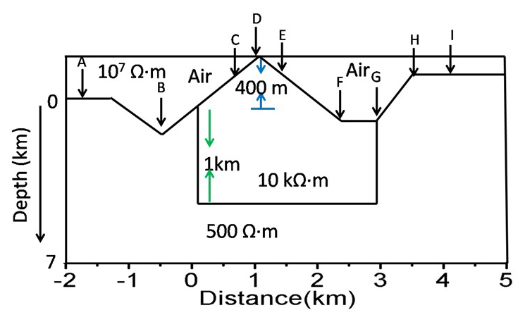
Figure 1 Topographic model of a 500 Ω m half-space with a resistive body of 10 kΩ m that was embedded from the surface relief (Chouteau and Bouchard, 1988).

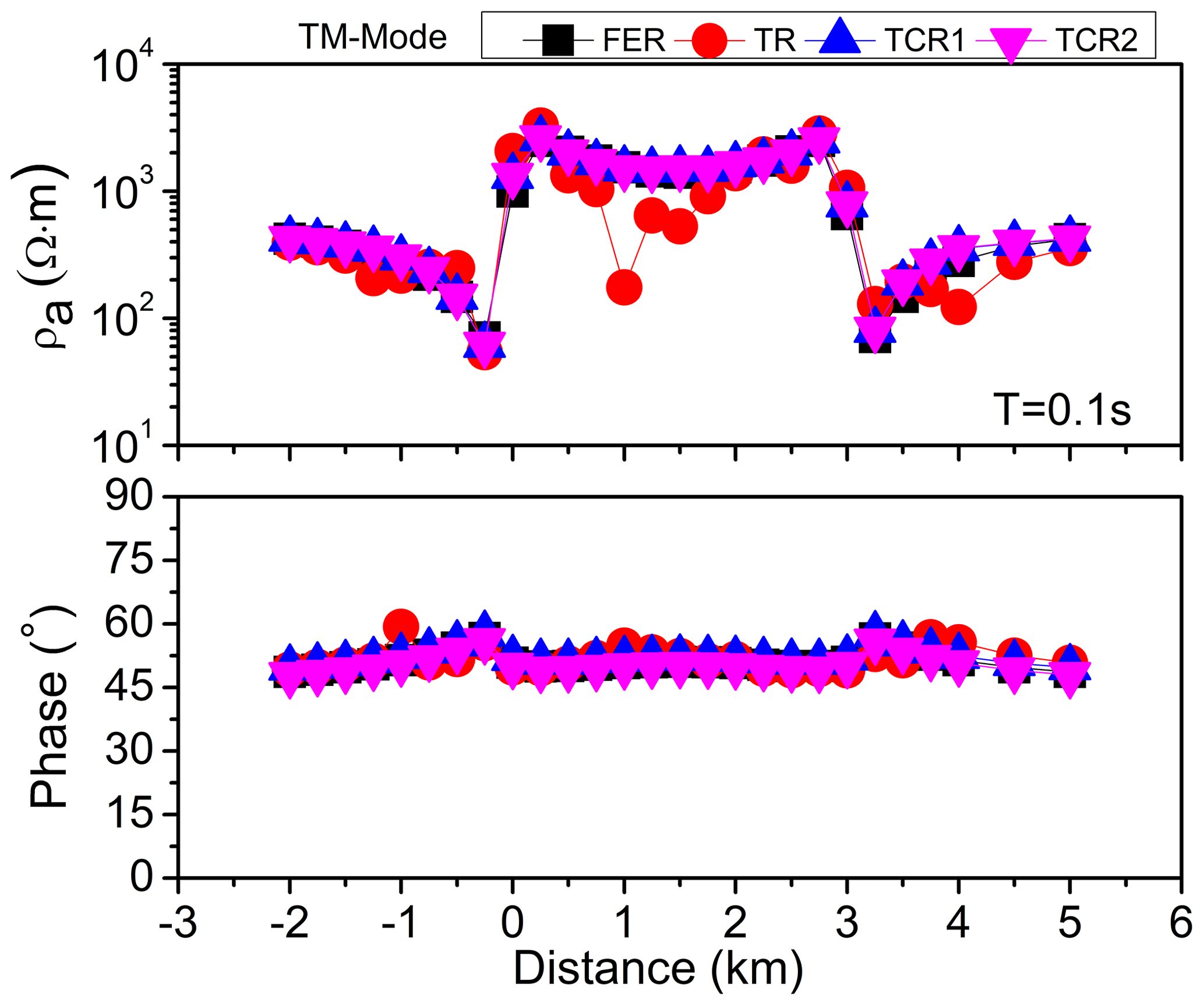
Figure 2 Comparison of the TM component of the flat-earth response (FER), topographic response (TR), and two terrain correction responses (TCR1 and TCR2) at 0.1 s.

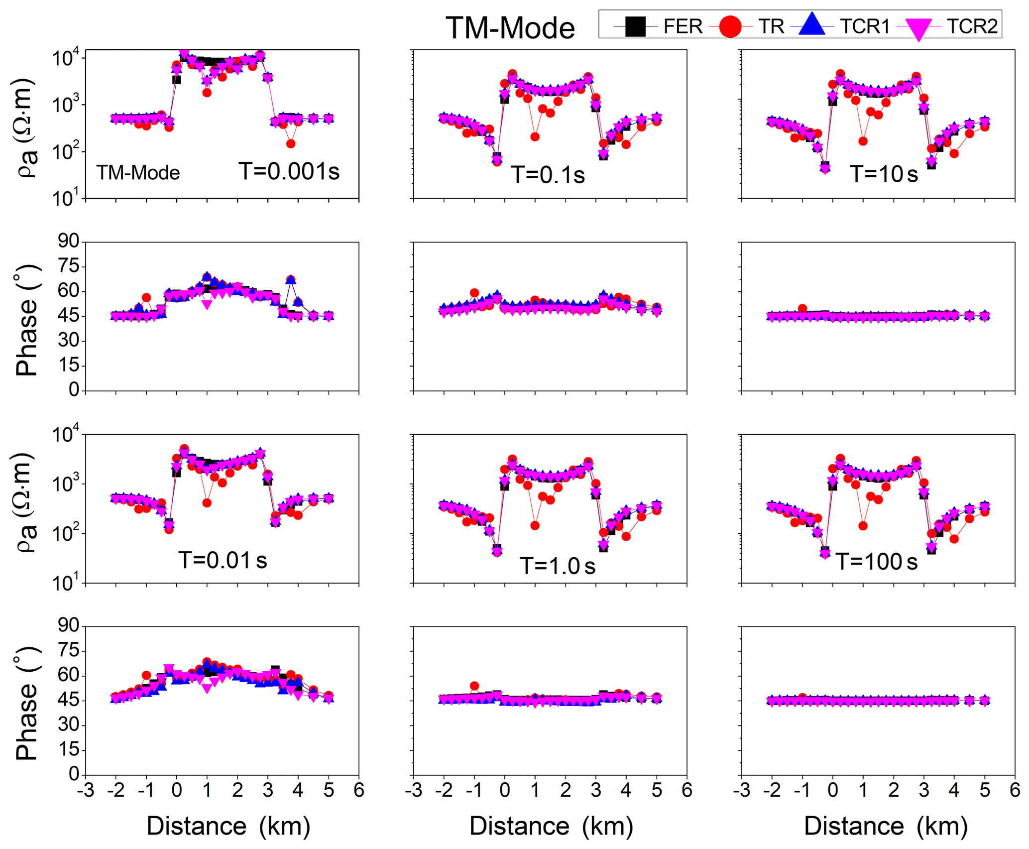
Figure 3 Comparison of the TM component of the flat-earth response (FER), topographic response (TR), and two correction procedures (TCR1 and TCR2) for the model in Fig. 1 for six different periods (0.001, 0.01, 0.1, 1, 10, and 100 s).

Figure 3 shows that the topography distortions are large for a longer period in the apparent resistivity component only, which presents the galvanic nature of the topography distortions. The terrain-corrected responses (TCR1 and TCR2) in Fig. 3 are almost similar to FERs for six respective periods (0.001, 0.01, 0.1, 1, 10, and 100 s). Relative errors were also calculated to check the accuracy of the terrain correction responses (TCR1 and TCR2) against FERs for these periods. The relative error between the FERs and TCR1 and TCR2 were very small for all periods except at site D only for shorter periods (because of the 10 kΩ m resistive body), as shown in Fig. 4. This shows the accuracy of the correction procedures.

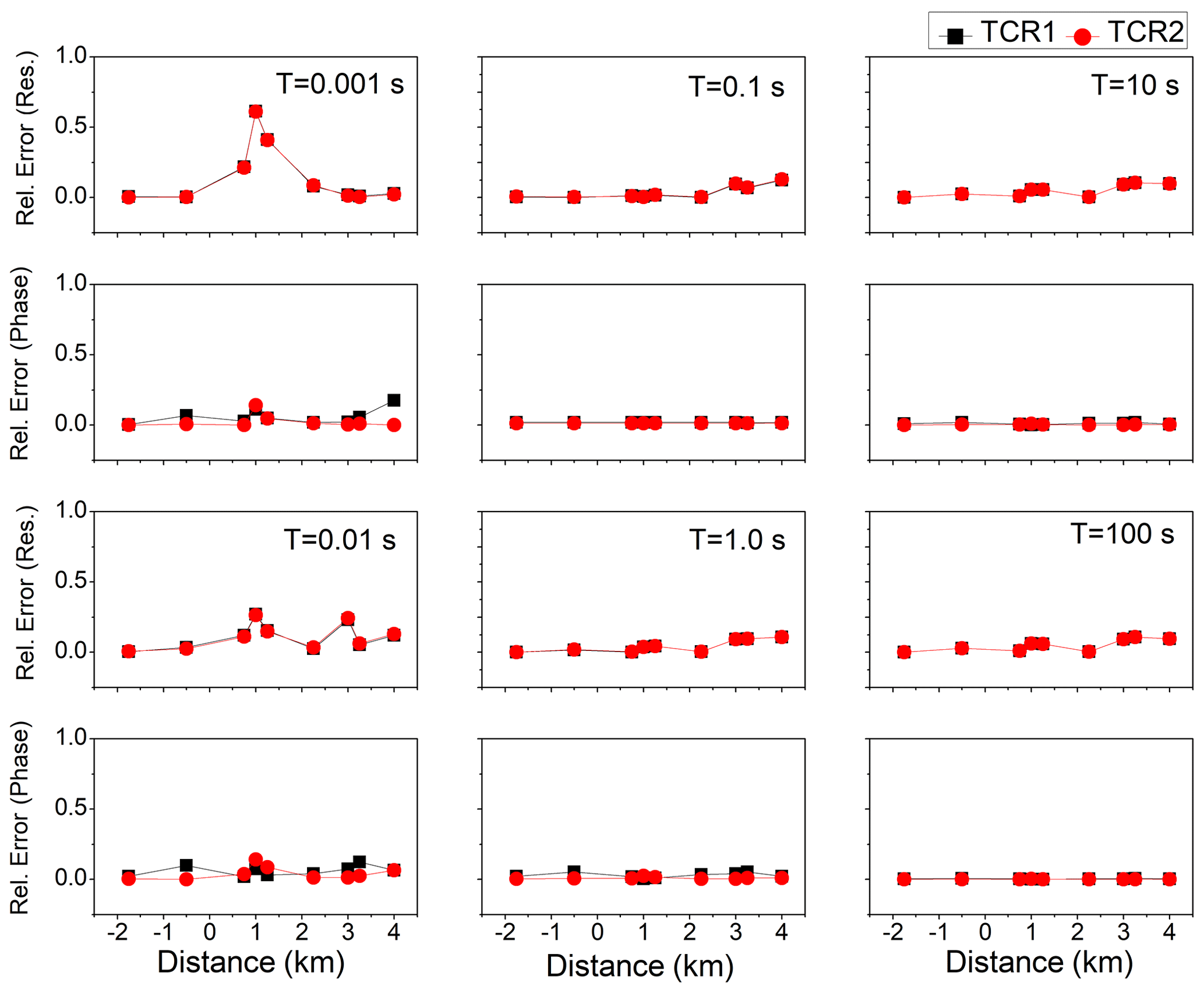
Figure 4 Relative error between terrain-corrected responses (TCR1 and TCR2) with respect to flat-earth responses (apparent resistivity and phase) for six different periods with a homogeneous half-space of 500 Ω m resistivity.

4 Modelling of the Roorkee–Gangotri section

A theoretical analysis of the effect of topography on MT responses was also taken into account in the Himalayan topography model. A theoretical model of the Roorkee–Gangotri profile was generated to simulate the MT response. To compute the MT forward modelling responses over a rugged topographic surface in the Roorkee–Gangotri section, the input model was prepared from a 2D inverted geoelectrical resistivity model (Tyagi, 2007). The topography model, with an elevation of 2.75 km, consists of a 180 km long profile drawn from Roorkee to Gangotri (Tyagi, 2007; Suman et al., 2023). In this model, two conductive blocks with a respective resistivity of 30 and 10 Ω m were embedded in a homogeneous half-space of 100 Ω m resistivity. The first block of 30 Ω m resistivity with a width of 80 km and a thickness of 6 km was embedded just near the Earth's surface relief and the second block of width 40 km and a thickness 25 km was embedded at 6 km depth from the surface. The MT responses were computed by considering three models: (1) one with a half-space of 100 Ω m resistivity (Fig. 5a), (2) one with a half-space of 500 Ω m resistivity, and (3) one with an additional resistive body of 8000 Ω m embedded from Earth's surface relief with a thickness of about 6 km and a half-space of 100 Ω m resistivity, as shown in Fig. 5b. The TR, FER, and two topography-corrected responses (TCR1 and TCR2) were analysed for nine sites (A, B, C, D, E, F, G, H, and I), as shown in Fig. 5, for six distinct periods (0.0013, 0.0102, 0.1063, 1.1110, 11.6078, and 121.2813 s).

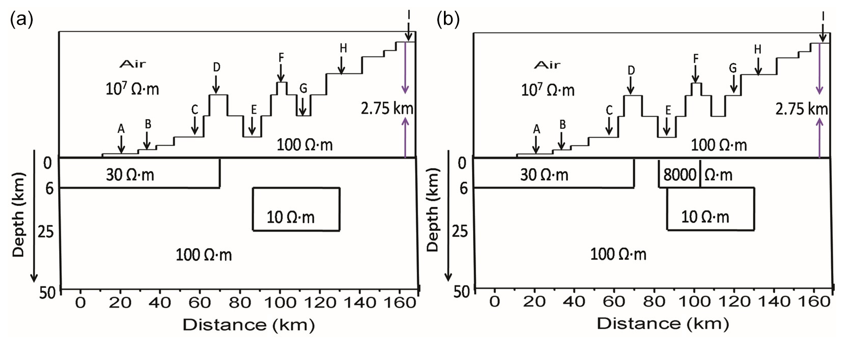
Figure 5 (a) A synthetic model of the Garhwal Himalaya region along the Roorkee–Gangotri profile in a half-space of 100 Ω m resistivity (b) with a resistive block of 8000 Ω m resistivity.

5 Result and discussion

5.1 Model with a half-space of 100 Ω m resistivity

The TR and FER were computed for the topography model with a conductive body of 30 Ω m resistivity in a half-space of 100 Ω m resistivity (Fig. 5a), and the topography corrections procedures were applied to the MT data. Figure 6 shows the TM mode of TR, FER, and two topography correction responses (TCR1 and TCR2) for six different periods (0.0013, 0.0102, 0.1063, 1.1110, 11.6078, and 121.2813 s). The topography effect depends upon the ramp/slope angle of the hill and is significant when the slope angle is greater than 7.5° (Kumar et al., 2018). It is clear from Fig. 6 that the TCR1 and TCR2 are almost similar to the TR, as the slope angle is less than 1°. The TCR1 and TCR2 were not similar to the FER for the sites from A to D for the shorter periods of 0.0013, 0.0102, 0.1063, and 1.1110 s, due to the exposure of the conductive body with 30 Ω m resistivity to the surface (from A to D) and its galvanic effect. The relative errors were also calculated between the FER with TCR1 and TCR2: they were high for the sites A, B, and C for shorter periods (0.0013, 0.0102, and 0.1063 s), due to the presence of the conductive body underneath these sites, and very small for all other sites (D, E, F, G, H, and I) for all periods, as shown in Fig. 7.

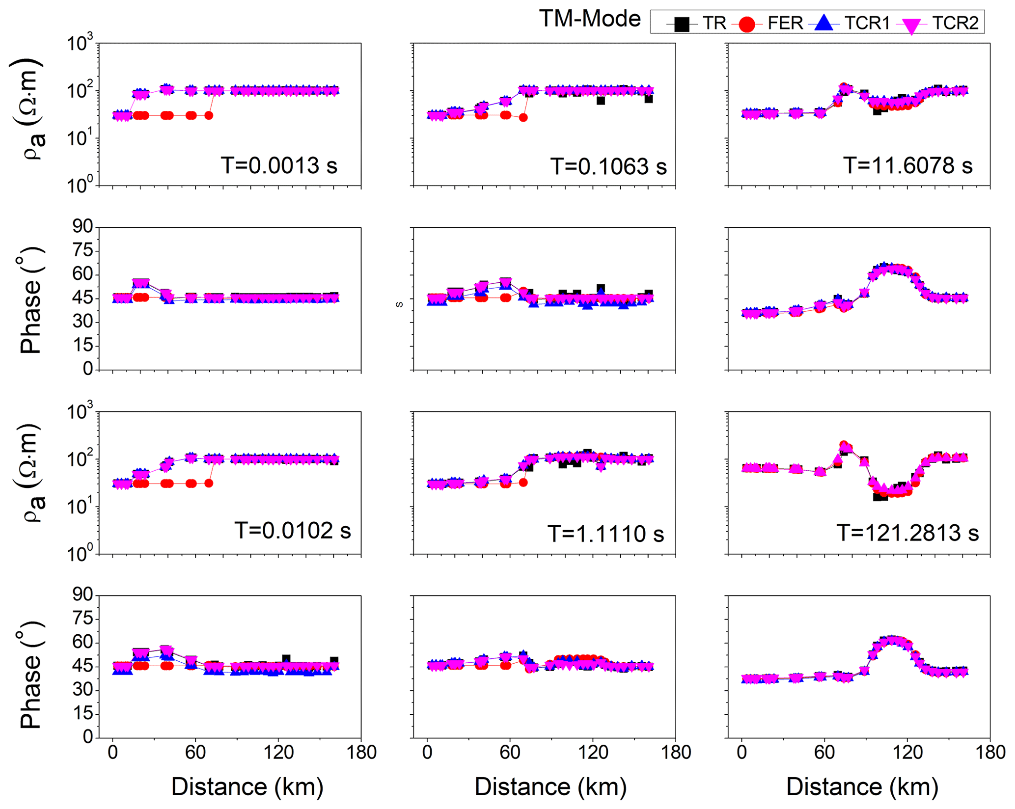
Figure 6 Comparison of the TM components of flat-earth response (FER), topographic response (TR), and two correction procedures (TCR1 and TCR2) for six different periods for a homogeneous half-space of 100 Ω m resistivity.

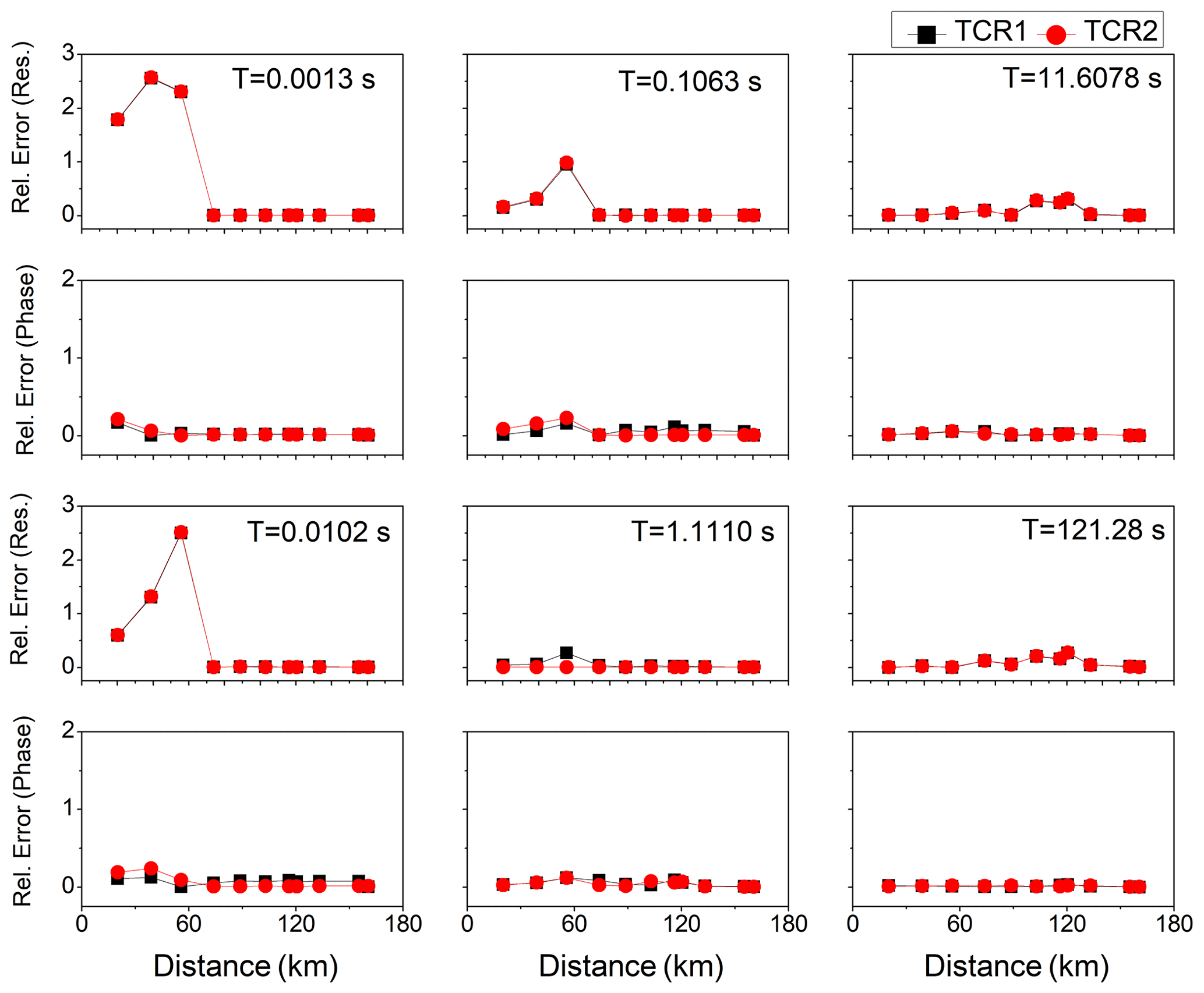
Figure 7 Relative error between the terrain-corrected responses (TCR1 and TCR2) with respect to the flat-earth response (apparent resistivity and phase) for six different periods with a half-space of 100 Ω m resistivity.

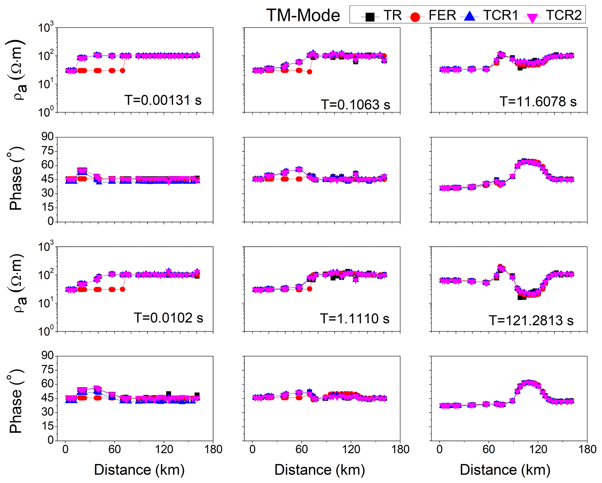
Figure 8 Comparison of the TM components of flat-earth response (FER), topographic response (TR), and two correction procedures (TCR1 and TCR2) for six different periods for a half-space of 500 Ω m resistivity.

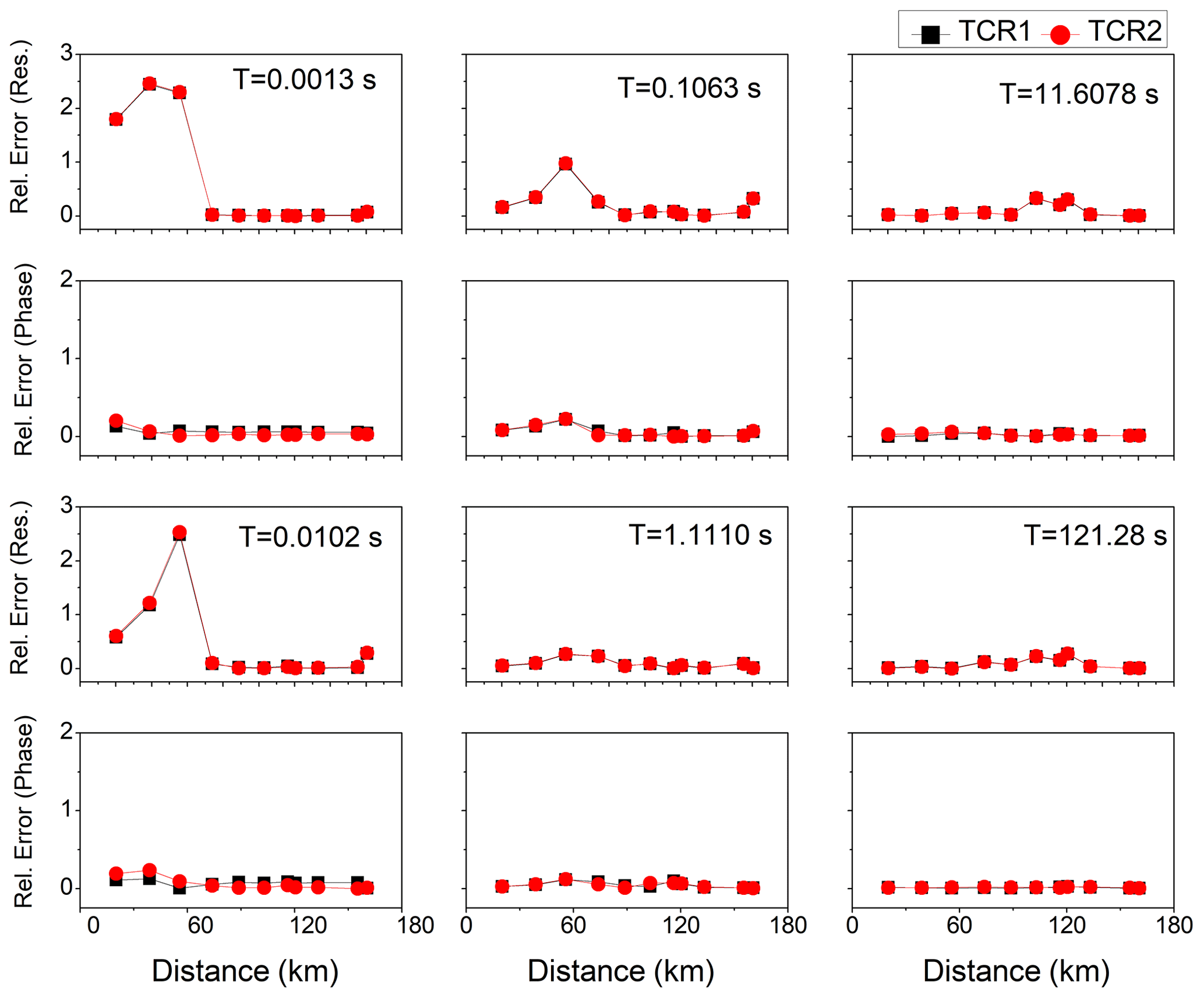
Figure 9 Relative error between the terrain-corrected responses (TCR1 and TCR2) with respect to the flat-earth response (apparent resistivity and phase) for six different periods with a half-space of 500 Ω m resistivity.

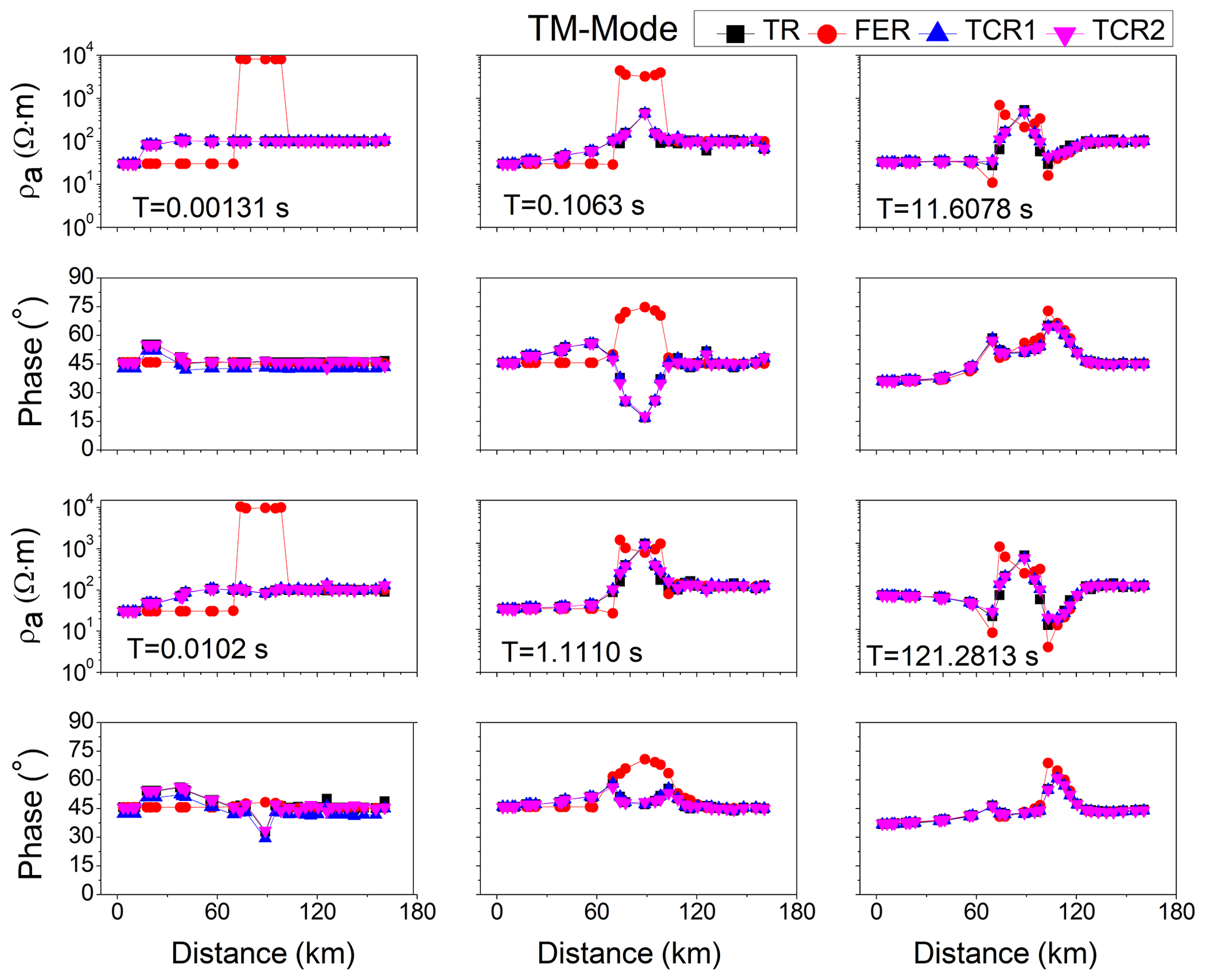
Figure 10 Comparison of the TM components of flat-earth response (FER), topographic response (TR), and two correction procedures (TCR1 and TCR2) for six different periods for a half-space of 100 Ω m resistivity.

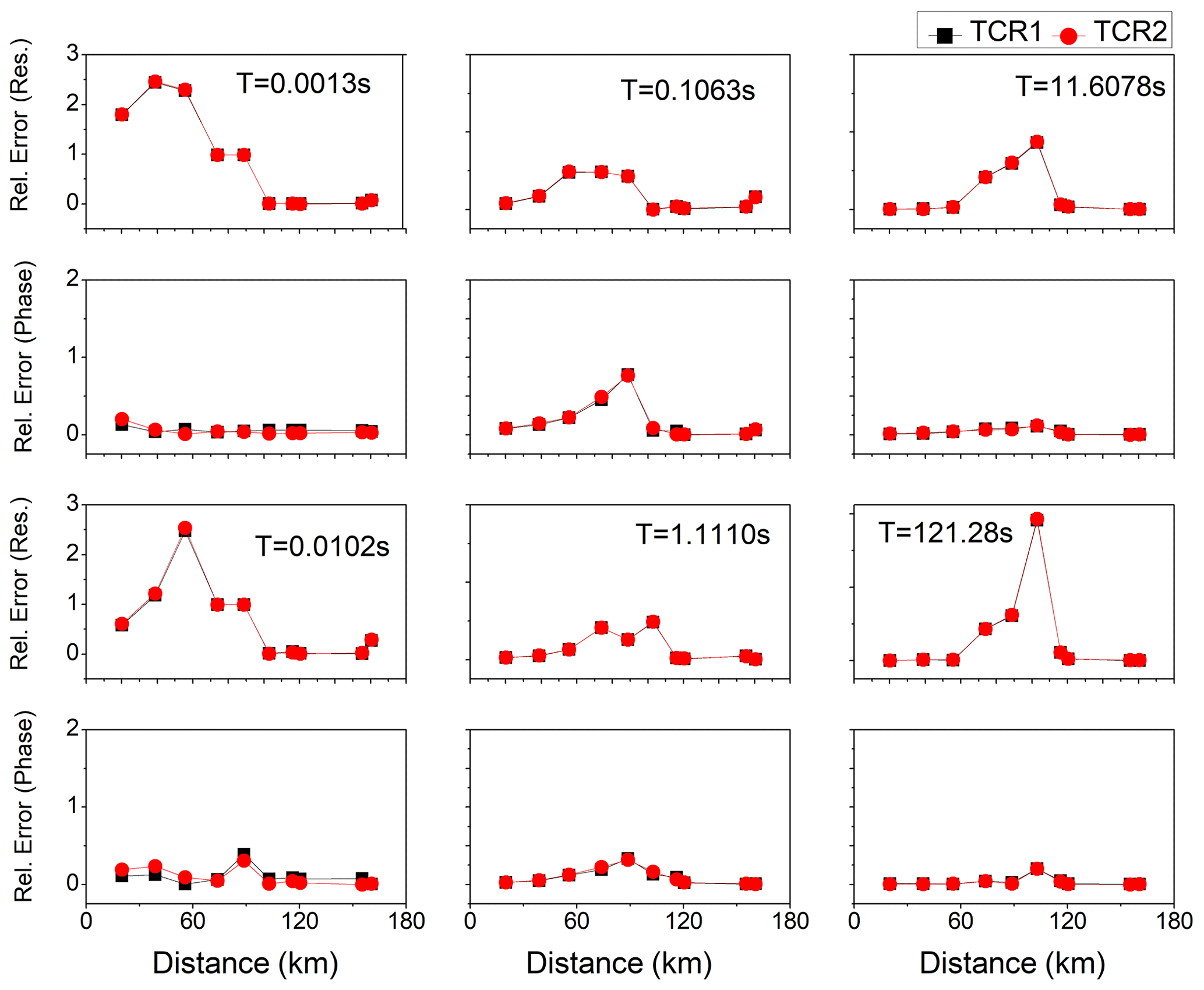
Figure 11 Relative error between the terrain-corrected responses (TCR1 and TCR2) with respect to the flat-earth response (apparent resistivity and phase) for six different periods with a half-space of 100 Ω m resistivity.

5.2 Model with a half-space of 500 Ω m resistivity

Now consider the case in which model half-space resistivity was replaced with 500 Ω m in Fig. 5a. The TR and FER were computed for the topography model with a half-space of 500 Ω m resistivity (Fig. 5a), and the topography correction procedures were applied to the MT data. Figure 8 shows the TM component of TR, FER, and topography-corrected responses (TCR1 and TCR 2) for six different periods. The results were almost similar to the response of the model with a half-space of 100 Ω m resistivity. The relative errors were also calculated in this case between the FER with TCR1 and TCR2, and the results were similar to the model with a half-space of 100 Ω m resistivity for all periods (0.0013, 0.0102, 0.1063, 1.1110, 11.6078, and 121.2813 s), as shown in Fig. 9.

5.3 Model with a resistive block of 8000 Ω m resistivity in a half-space of 100 Ω m resistivity

The TR and FER were also computed for the topography model with a resistive block of 8000 Ω m resistivity in a half-space of 100 Ω m resistivity (Fig. 5b), and the topography corrections were applied to the MT data. Figure 10 shows the TM component of TR, FER, and two topography correction responses (TCR1 and TCR2) for six different periods. The TCR1 and TCR2 were not similar to the flat-earth model for the sites from A to F, due to the exposure of the conductive body with a 30 Ω m resistivity to the surface (from A to D) and its galvanic effect as well as the presence of a 8000 Ω m resistive body (from D to F). The relative errors were also calculated between the FER with TCR1 and TCR2 and were high for the sites A, B, and C for shorter periods (0.0013, 0.0102, and 0.1063 s), due to the presence of the conductive body underneath these sites, and for longer periods (1.1110, 11.6078, and 121.2813 s), due to the presence of an 8000 Ω m resistive body from D to F, as shown in Fig. 11.

6 Conclusions

The study shows the effect of topography in the MT data along a synthetic model of the Roorkee–Gangotri profile. Two correction procedures were used to remove the topography distortion from MT data. The similar FER, TCR1, and TCR2 in Fig. 3 show that both correction procedures are capable of removing the topography effect and, thus, confirms the accuracy of the two correction procedures. The similar TR, TCR1, and TCR2 responses (Figs. 6, 8, 10) concluded that there is no need for topography correction along the Roorkee–Gangotri profile, as the slope angle is less than 1°. The relative error between the FER and TCR1 and TCR2 also showed the accuracy of the two correction procedures (TCR1 and TCR2) in this study. The presence of near-surface heterogeneity/surface exposure of conductive/resistive body also distorts the MT responses in this model (the FER is not similar to TR, TCR1, and TCR2).