the Creative Commons Attribution 4.0 License.
the Creative Commons Attribution 4.0 License.
 | 08 Mar 2023
Rain process models and convergence to point processes
Samuel N. Stechmann
A variety of stochastic models have been used to describe time series of precipitation or rainfall. Since many of these stochastic models are simplistic, it is desirable to develop connections between the stochastic models and the underlying physics of rain. Here, convergence results are presented for such a connection between two stochastic models: (i) a stochastic moisture process as a physics-based description of atmospheric moisture evolution and (ii) a point process for rainfall time series as spike trains. The moisture process has dynamics that switch after the moisture hits a threshold, which represents the onset of rainfall and thereby gives rise to an associated rainfall process. This rainfall process is characterized by its random holding times for dry and wet periods. On average, the holding times for the wet periods are much shorter than the dry ones, and, in the limit of short wet periods, the rainfall process converges to a point process that is a spike train. Also, in the limit, the underlying moisture process becomes a threshold model with a teleporting boundary condition. To establish these limits and connections, formal asymptotic convergence is shown using the Fokker–Planck equation, which provides some intuitive understanding. Also, rigorous convergence is proved in mean square with respect to continuous functions of the moisture process and convergence in mean square with respect to generalized functions of the rain process.
- Article
(1330 KB) - Full-text XML
- BibTeX
- EndNote


Time series of precipitation or rainfall display highly irregular behavior, as illustrated in Fig. 1, and many valuable models have been based on stochastic processes. A variety of different stochastic models have been used, including renewal processes, Markov chains, Poisson processes, and point processes (Green, 1964; Katz, 1977; Richardson, 1981; Smith and Karr, 1983; Foufoula-Georgiou and Lettenmaier, 1987; Rodriguez-Iturbe et al., 1988; Cowpertwait et al., 1996; Wilks and Wilby, 1999). The many applications of these models include weather forecasting, stochastic weather generation, climate impact assessment, climate model downscaling, hydrological modeling, ecological modeling, and agricultural modeling.
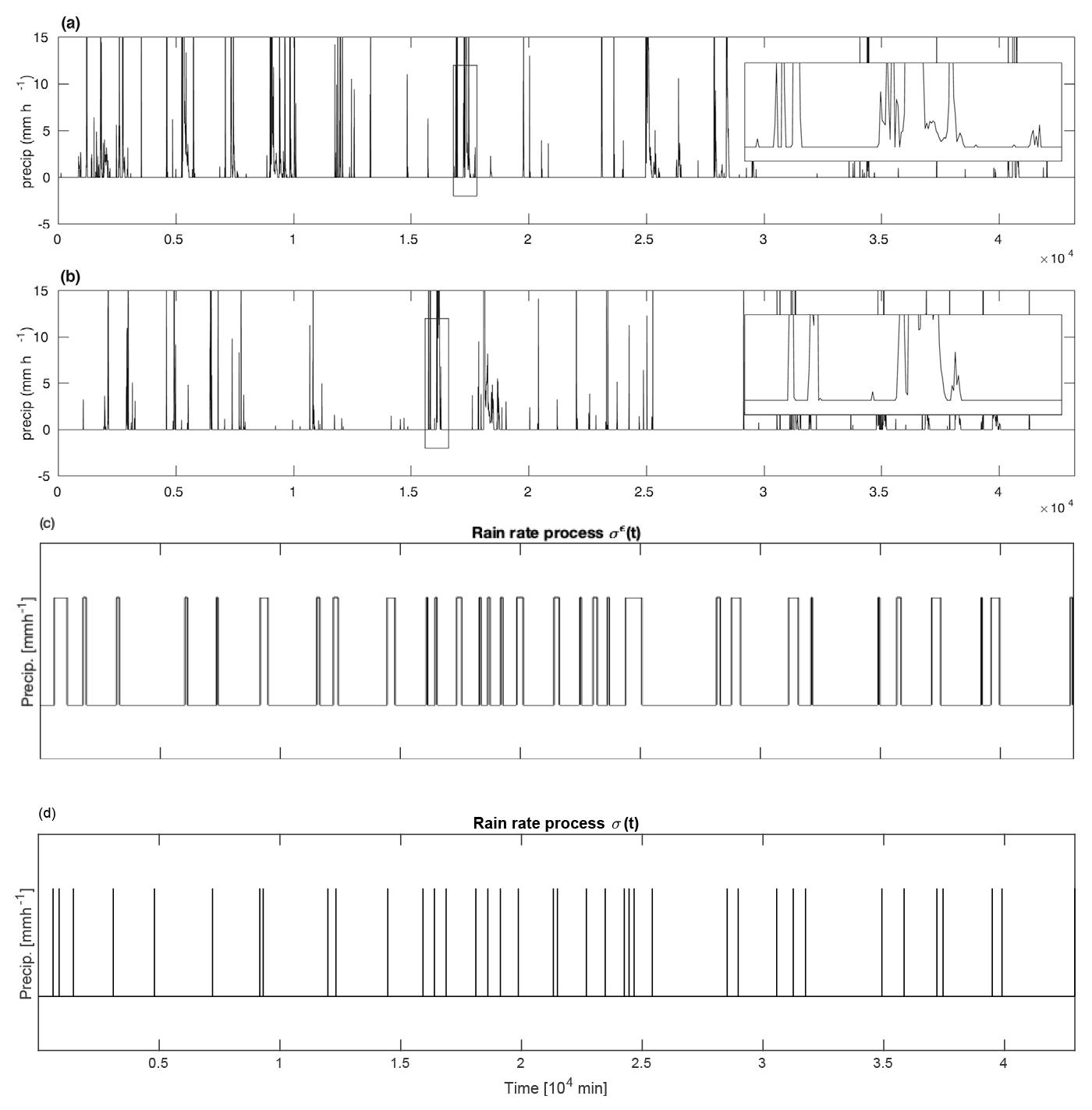
Figure 1Sample precipitation time series from observations at (a) Manus Island and (b) Nauru reproduced from Fig. 3 of Abbott et al. (2016) with permission from the authors. The latter two panels are stochastic model simulations of (c) the rain rate process σϵ(t) with finite rain rate r and (d) σ(t) as the point process.
Commonly, stochastic models for rainfall are empirical – i.e., based mainly on fitting the model behavior to match observational rainfall data – rather than based mainly on the underlying physical laws. Nevertheless, it is desirable to relate the stochastic models to physical principles, to the extent possible. Here, we investigate such a relation.
In particular, the goal of the present paper is to prove a connection between (i) a point-process description of rainfall time series and (ii) a physics-based model for the stochastic evolution of moisture. At first glance, the point-process model appears to be somewhat disconnected from basic physical laws based on mass, momentum, and energy. However, the point-process model can be seen to arise from the underlying evolution of moisture (which is the mixing ratio of water vapor in the air) (Abbott et al., 2016). Here, this connection is demonstrated via formal asymptotics on the Fokker–Planck equation and proved rigorously in the mean-square sense.
To be more specific, a point-process model of rainfall can be viewed as a spike train, as in Fig. 1d, where a rainfall event is an instantaneous spike. The point process could be defined and characterized by the random waiting time, τd, of the duration of the “dry spell” in between rain events. As an empirical model of rainfall, one could estimate the probability density function (pdf) of τd based on observational data (Peters et al., 2010; Deluca and Corral, 2014). For such an empirical approach, one could use data of rainfall time series alone, without appealing to any physical laws or any other type of observational data (humidity, wind speed, etc.). Similarly, beyond point processes, one could use a renewal process as a model of rainfall time series, as in Fig. 1c, by introducing a finite (and possibly random) time τr for the duration of the rain event. Again, as in the case of a point process, one could use a renewal process as an empirical model, based on data of rainfall time series alone, without appealing to any physical laws or any other type of observational data. However, it would be desirable to show that the point-process and renewal-process models can also arise from more physically based underpinnings.
Here, as mentioned above, a point-process model of precipitation will be linked to the evolution of moisture to provide a more physically based foundation of the point-process model. The moisture model used here is a continuous-time stochastic process for q(t), which represents the amount of water vapor in a column of the atmosphere, as an anomaly from a baseline level, at time t (Stechmann and Neelin, 2011, 2014; Hottovy and Stechmann, 2015b; Abbott et al., 2016; Neelin et al., 2017). For example, the anomaly q(t)=0 corresponds to 62 mm of moisture in the column, and mm will be an upper threshold of 65 mm of moisture in the column.
The q(t) process is governed by the stochastic differential equations (SDEs)
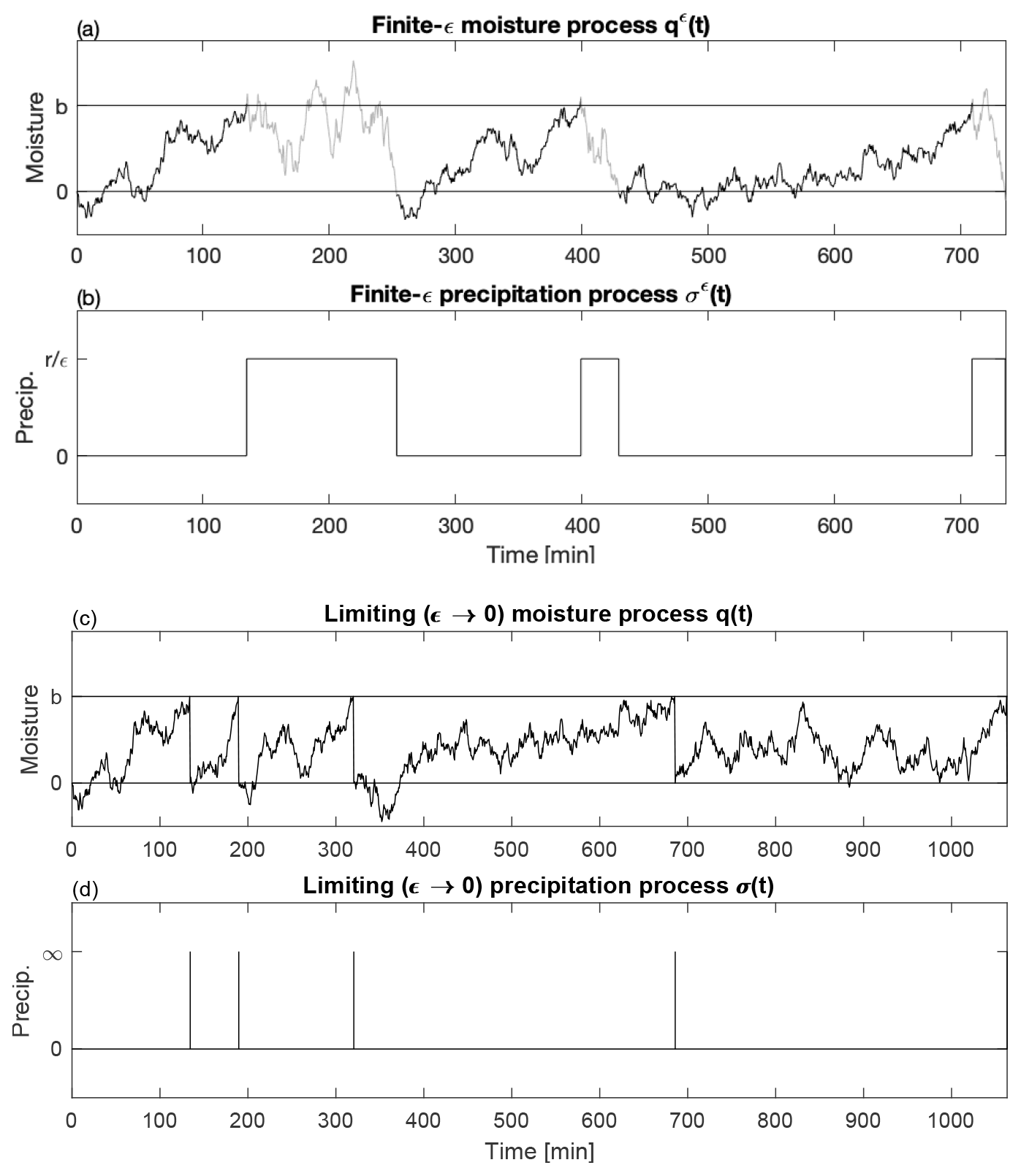
where m and r are the moistening and rain rates, respectively, and D0 and D1 are the constant diffusion coefficients which capture the fluctuations of moisture during the respective states and Wt is a standard Wiener process. The quantity σ(t) is an indicator function for rain, and the dynamics of σ(t) switch from 0 to r when q(t) reaches a fixed threshold b>0. For instance, supposing that , then σ(t)=0 until the time , at which time the value of σ switches to σ(t)=r. Then σ(t) switches back to zero at a later time when the moisture has been depleted to the lower threshold (q(t)=0). Figure 2a, b show a realization of the processes q(t) and σ(t). The process σ(t) can be viewed as a renewal process, with random durations τd and τr of dry spells and rain events, respectively, although σ(t) is not just a standalone renewal process, since it arises from the underlying dynamics of moisture q. The moisture in the column can potentially reach negative values, i.e., , on very rare occasions. This effect is due to the idealized nature of the model.
The threshold behavior of Eq. (1) is a fundamental feature of the moisture–rainfall relationship that is seen in nature (Peters and Neelin, 2006; Deluca et al., 2015), and it is a basic aspect of many more complex moisture models and convective parameterizations as well (Lin and Neelin, 2000; Frierson et al., 2004; Khouider and Majda, 2005; Khouider et al., 2010; Hottovy and Stechmann, 2015a; Stechmann and Hottovy, 2016; Ahmed and Neelin, 2019; Mueller and Stechmann, 2020; Huang et al., 2022). Sometimes the threshold is also called a trigger (Hernandez-Duenas et al., 2019). The threshold can be viewed as the threshold for the release of moist convective instability, and the moisture q is used as the physical quantity that governs the onset of moist convection. In this way, Eq. (1) is a physically based model of atmospheric moisture, and, from it, one can obtain a rainfall time series as a secondary or auxiliary quantity.
The main purpose of the paper is to define and show convergence of the threshold model in Eq. (1) as r→∞ to a point-process model of rainfall. For example, on the level of renewal processes, τr→0, and thus σ(t) converges to a process that is zero everywhere and that has spikes at infinity after random durations of length τd. That is, σ(t) converges to a Dirac delta process. However, σ(t) is right-continuous and has left-hand limits, whereas the spike train is not. Thus, the mode of convergence is not clear. For q(t) the limit is also unclear but will be redefined in a way to show convergence with respect to the topology on continuous functions with the uniform metric. In this study, the limiting processes are defined (in Sect. 2), and convergence is shown both heuristically (for the Fokker–Planck equation) and rigorously.
Some of the novel aspects of this work are as follows. The limit jump process q(t) has an associated Fokker–Planck equation that is derived using a matched asymptotic method. The resulting Fokker–Planck equation has a peculiar boundary flux condition which defines a “teleporting” boundary condition of q(t). The processes are decoupled into evaporating and precipitating processes. Only after this decoupling can convergence of the evaporation processes be shown rigorously with respect to the uniform metric on the space of continuous functions. Also, the rain process σ(t) is shown to converge rigorously with respect to the generalized function space. This proof shows convergence of a renewal process to a delta process. Furthermore, the proof shows what kinds of bounds are needed for the rain event times τr in order for integrated convergence to hold.
The convergence results shown here have the potential to impact various other fields. Many fields of study use similar renewal processes to model different types of phenomena (Cox, 1962). The connections to rain models were made above. In addition, there has been work in queuing theory to approximate point processes with renewal processes (e.g., Whitt, 1982; Bhat, 1994) and using threshold triggers in financial models (Lejay and Pigato, 2019). Thresholds arise in many applications of piecewise dynamical systems where the threshold marks a change in the dynamics, as in Fillipov dynamics and hybrid switching diffusions (Filippov, 2013; Simpson and Kuske, 2012). The limiting process is similar to a stochastic resetting process studied in Evans and Majumdar (2011) and Evans et al. (2020). Here the process stochastically resets to q=0 after a random hitting time τd which depends on the process. Another interesting connection is with neuron stochastic integrate and fire models (see Sacerdote and Giraudo, 2013, for a review). The moisture process with a finite rain rate is similar to a Wiener process model of a single neuron with refractoriness. A similar model was studied in Albano et al. (2008), where the refractory time was constant. Here, the refractory time is random and coincides with the rain duration time τr. Thus, the work here is applicable to understanding the differences in using a model without refractoriness versus a model with a short, possibly random, refractory time.
The structure of the paper is as follows. The processes for moisture and rain are defined in Sect. 2. The modes of convergence are discussed in Sect. 3. The heuristic convergence with the Fokker–Planck equation is shown in Sect. 3.1. Rigorous convergence of the moistening process Eϵ to E is shown with respect to L2 in Sect. 3.2, and the rain process σϵ is shown to converge to the sum of delta distributions σ with respect to generalized functions in Sect. 3.3. Some important statistics as well as an analysis of the differences when using the two processes are shown in Sect. 4. The results are summarized in Sect. 5. Technical details of the proofs and derivations are given in the Appendix.
In this section the moisture and precipitation processes are defined. First, the underlying moisture process of the renewal rain process is defined. The processes are defined with a small parameter ϵ with the limit as ϵ→0 in mind.
The moisture process qϵ(t)∈ℝ is defined as the solution to the SDE,
where m and are the moistening and rain rates, and are the fluctuations of moisture during the respective states. Here the small parameter ϵ is essentially the ratio of moistening and rain rates (times a constant O(1) factor). In other words, ϵ is the value which makes order 1. In the tropics, the rain rate is often seen to have values in excess of 15 mm h−1 (e.g., see Fig. 1a and b). See Fig. 7a in Holloway and Neelin (2010) for an estimate of a typical moistening rate in the tropics. There the moistening rate is roughly 0.4 mm h−1. The rain process is defined as follows: since σϵ(0)=0, let . Then σϵ(t)=0 for . Next, let and for . This process repeats up to an arbitrary final time T. Define the time intervals and as
and so on. These are the duration times for dry and rain events, respectively.
The associated processes, as ϵ→0, are defined as q(t) and σ(t) for the moisture and rain processes. (It would perhaps be appropriate to denote the limiting processes as q0(t) and σ0(t), to indicate that they arise from qϵ(t) and σϵ(t) in the limit ϵ→0. However, we will drop the superscript 0 from q0(t) and σ0(t) to ease notation.) The moisture process is the solution to the SDE
with the unusual boundary condition as follows: let the usual stopping time be . Then, at time t=𝒯1, the process q(t) jumps or “teleports” to q=0. However, the function is defined as both 0 and b at 𝒯1. For convention, the process is defined as cadlag (continuous from the right with left-hand limits), i.e.,
Then the process starts over using the dynamics of Eq. (4) until , and the process repeats. The time intervals
are the dry event durations. The rain event duration, on the other hand, is not defined for this limiting process, since rain events are instantaneous in the intense-rain-rate limit of ϵ→0.
Example time series of the processes are shown in Fig. 2. The processes with finite rain rate for ϵ>0 are shown in panels (a) and (b). Panel (a) is the moisture process qϵ(t) defined in Eq. (2). The rain rate process is shown in panel (b) and takes the value when qϵ(t) reaches level b for the first time (panel a in black) and resets to zero when qϵ(t) reaches zero (panel a in gray). This process repeats. The limiting processes are shown in panels (c) and (d). Panel (c) shows the limiting moisture process q(t) defined in Eq. (4), and panel (d) shows the rain process defined in Eq. (7). The moisture process is a Brownian motion with positive drift until reaching level b. When q(t)=b, the process σ(t) takes an infinite value, and the moisture process is reset to zero.
From the definition of above, the rain point process σ(t) is defined as
where 𝒩(T) is the random variable of the number of times the process q(t) reaches b in time T. The quantity b arises because the moisture process qϵ loses moisture at a rate of per time, on average. The moisture process q(t) loses all the moisture built up (which is an amount b) instantaneously.
Note that qϵ(t) has continuous paths, while q(t) has jump discontinuities. Thus, any mode of convergence between qϵ and q with an associated metric (e.g., uniform or Skorohod) will fail (Kelley, 2017). Nevertheless, there is another way to define both qϵ and q in which convergence with respect to L2 with the uniform metric on the space of continuous functions (𝒞[0,T]) can be shown. To do so, qϵ(t) is decomposed into an evaporating process, Eϵ(t), and precipitating process, Pϵ(t). These processes are defined as
Thus, the moisture process qϵ(t) is written as
In the limit, the jumps will be captured in the Pϵ process. In the following section it will be shown (see Sect. 3.2) that Eϵ→E, where E(t) is defined as the solution to the SDE
Furthermore, the spike times of the σ process, which was defined above in Eq. (7), could now also be defined in terms of the E(t) process as , i.e., the first passage time of Brownian motion with drift to ib.
In this section convergence is shown both heuristically (e.g., Sect. 3.1) and rigorously (e.g., Sect. 3.2 and 3.3).
Note that the simplest ideas of convergence break down when considering pathwise convergence of qϵ to q and σϵ to σ. This is because qϵ is a continuous process for all ϵ>0, whereas q is a process with jumps, σϵ is left-continuous with right-hand limits, and σ is no longer left-continuous. Thus, there is no topology with the associated metric d such that qϵ→q with respect to d (Kelley, 2017). However, one could try to show that qϵ converges in a notion weaker than the Skorohod topology; see Kurtz (1991) for these conditions. Such convergence would happen in a topology which does not have an associated metric (see Jakubowski, 1997). This approach is not pursued here as it is technical and does not give any insight into the model or approximation.
Instead, we pursue convergence in the following senses. The next three subsections prove convergence of the various processes introduced in Sect. 2. In Sect. 3.1 the Fokker–Planck equation for qϵ is shown to converge (formally) to a Fokker–Planck equation for q. This derivation gives rise to an interesting partial differential equation (PDE) with unusual “teleporting” boundary conditions. In Sect. 3.2 convergence in paths is shown for Eϵ to E with respect to the uniform metric for continuous functions on [0,T]. In Sect. 3.3 convergence is shown for σϵ to σ with respect to generalized functions. This norm is necessary because σ is a sum of Dirac delta functions. In addition, this convergence is natural to consider for applications where the errors are analyzed between using σϵ and a point process (σ) in, for example, a climate model or as a model for observational time series.
3.1 Fokker–Planck equation
In this section, we derive the Fokker–Planck equation of Eq. (4) by taking the formal asymptotic limit, as ϵ→0, of the Fokker–Planck equation of Eq. (2). This mode of convergence provides some intuition for the behavior in the ϵ→0 limit.
The Fokker–Planck equation for Eq. (2) (see Hottovy and Stechmann, 2015b) is composed of two densities. These densities are denoted ρ0 and ρ1 for the dry state (σϵ=0) and the rain state (σϵ=1), respectively. These densities evolve according to the following Fokker–Planck equations:
where the fluxes fi are defined as
and with the following conditions,
which are absorbing boundary conditions and the normalization condition, respectively. This implies that once the particle reaches q=b (or q=0), the particle is removed and added to the state σ=1 (or σ=0) (Gardiner, 2004). Thus, the particle reaches q=b but cannot be found there: . Note that the flux terms in Eqs. (12a) and (12b) contain ρ0,ρ1 terms and their derivative. If the derivatives are zero, then the absorbing boundary conditions would imply that the Dirac delta coupling terms in Eqs. (10) and (11) are zero. However, this is not the case. The Fokker–Planck equation must be solved on three separate intervals of , [0,b], and [b,∞). This leads to points of non-differentiability for ρ0 and ρ1 at q=0 and q=b. For an example, see the stationary solutions in Sect. 4 and Fig. 3.
To obtain Eqs. (10) and (11), a further approximation is used. In Hottovy and Stechmann (2015b), q(t) is modeled similarly to Eq. (2), except that the σ process switches states at a random time with rate λ after q(t) reaches the threshold. Call this process qλ(t). The Fokker–Planck-type equation for qλ(t) uses terms from the master equation (see Gardiner, 2004, Sect. 3.5). The Fokker–Planck equation in Eqs. (10) and (11) is derived by taking an asymptotic of the equations for qλ and taking a limit as λ→∞, that is, as the random switching time becomes small.
One interesting property of these Fokker–Planck equations is the appearance of Dirac delta source terms, which represent transitions between the dry state and the rain state. For instance, in Eq. (10), a Dirac delta source term arises at q=0, and it represents the transition from the rain state (σϵ=1) to the dry state (σϵ=0) when the (raining) moisture process reaches the lower threshold at q=0. The magnitude of this Dirac delta source term is , which is the outward flux of ρ1 at the lower threshold, q=0, as defined from Eqs. (11) and (12b).
The proposed limit as ϵ→0 for the Fokker–Planck equation is
with the following conditions:
This Fokker–Planck equation is much different than the coupled system of Eqs. (10)–(11). For example, the coupled system is defined for all , whereas Eq. (15) is only defined for . This is because the boundary q=b becomes impassable due to the teleporting boundary, or, in physical terms, the rain rate is so strong that the moisture q moves above the threshold b by only a small O(ϵ) amount that vanishes as ϵ→0. The restriction of q can be seen in the stationary densities in Sect. 4. There, the stationary density for state σϵ(t)=1 decays to zero quickly. Another interesting property of this Fokker–Planck equation is that the absorbing boundary condition at q=b in Eq. (17) is actually coupled to a Dirac delta source at q=0 in the Fokker–Planck Eq. (15). In this coupling, the flux of absorption at the boundary is also equal to the magnitude of the source which inserts mass at q=0. Therefore, when the process is absorbed at q=b, it is reinserted at q=0, and in this way it represents a teleporting boundary condition.
The convergence of the time-dependent Fokker–Planck Eqs. (10)–(11) is shown through an asymptotic expansion in the Appendix. The analysis is shown for the full time-dependent Fokker–Planck equation to show that the transient solutions to these equations also converge as The method used is a matched asymptotic expansion argument (Bender and Orszag, 2013). This argument shows how the interesting delta function condition of the probability flux arises in Eq. (15).
3.2 Pathwise convergence
Rigorous mathematical convergence is now considered. For this section and the next, a useful lemma is first stated and proved. In essence, the lemma states that, for a finite time interval [0,T], it is (exponentially) unlikely that a large number of rain events will occur.
Let 𝒩ϵ(T) be the number of rain events for the qϵ process defined in Eq. (4). Then, for ,
The proof of the lemma is contained in the Appendix. This lemma shows that the probability of N events decays exponentially in N. With this lemma, pathwise convergence is now considered. Recall from the discussion at the beginning of the section that we consider convergence not for qϵ, but for the evaporating process Eϵ. Convergence from Eϵ to E is shown in L2(Ω) with respect to the uniform metric on the space of continuous functions C[0,T].
This theorem shows that the moistening process Eϵ converges to the process E as Furthermore, the moistening process E contains all the dynamics of the joint (E,σ) process. The rigorous proof is shown in the Appendix. The proof relies on the processes Eϵ and E being driven by the same white noise process. Thus, they converge to each other by showing that the first two moments of τr,ϵ converge to zero (see Eq. A27).
3.3 Distributional convergence
In this subsection L2(Ω) convergence of σϵ to σ is shown with respect to a generalized function norm. This norm is considered here due to the nature of the delta function. It is also a natural norm to consider as it is an integrated error. That is, this norm considers the accumulation of errors after running the model for time T>0.
The technical details of the proof are given in the Appendix. The procedure is similar to the proof of Theorem 1. However, here the case for different numbers of rain events in the time interval for the processes σ and σϵ must be considered in a different way (see Eq. A45). This leads to needing estimates of the first four moments of the event duration τr,ϵ.
In this section, important statistics and applications of the processes (qϵ,σϵ) and (q,σ) are presented. These statistics show the differences between the processes and give motivation for the approximations. These include the stationary Fokker–Planck solution, the rain and dry event distributions, the rain fraction, and an application of Theorem 2.
4.1 Stationary Fokker–Planck equation
Here the analytical solutions to the stationary Fokker–Planck equation are given. The stationary Fokker–Planck equation for the process qϵ is
with the conditions
The analytical solutions are found in Hottovy and Stechmann (2015a) and are reproduced here. They are
and similarly for The densities are plotted in Fig. 3. The black curve is the density for one value of For the other masses changes very little (order ϵ) and is not shown. The density is plotted in gray for various values of ϵ. The density is scaled by ϵ−1. The dashed gray line is the limiting shape. Thus, as ϵ→0, the density is a uniform distribution on the interval [0,b] that tends to zero. Note that the absorbing boundary conditions from Eq. (24) are satisfied ( and ). However, their derivatives (the fluxes) are nonzero. Thus, the Dirac delta terms in the Fokker–Planck equation are nonzero.
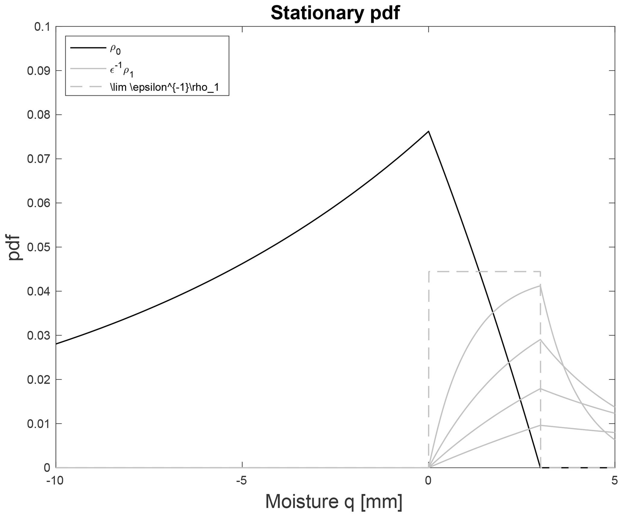
Figure 3Stationary probability density functions (pdfs) for the density (black line) and density for values of and 0.1 (gray lines). The dashed line is the limit shape of the density scaled by ϵ−1.
4.2 Event duration
Another statistic studied here is the event duration probability density. This density gives information on the probability of a dry/rain event lasting time t minutes. For the process qϵ, both the dry and rain states are Brownian motions with drift (m for dry and for rain). Thus, the event duration densities are the first passage to q=b densities for Brownian motion with drift (Gardiner, 2004, Sect. 5.5.1). These densities were found in Stechmann and Neelin (2014) and are reproduced here. The event duration density for a rain event is
and similarly for the dry event duration ρ0t. The density for rain events changes with ϵ, while the dry event density does not. The rain event duration has cutoffs for short and long times. They are
The short-time cutoff is independent of ϵ, while the long-time cutoff tends to zero in O(ϵ2). This implies that for smaller ϵ, the extreme events are being cut off quickly. Hence, in the ϵ→0 limit, extreme rainfall events do not occur. In order to preserve extreme rainfall events in a point-process model of rainfall, the rain rate amplitude would need to be modeled as a stochastic process, since rain event durations are assumed to be short (see Sect. 4.5).
These densities are plotted in Fig. 4 on a log–log scale. The dry density ρ0t is the black curve. The rain event duration density ρ1t is plotted in gray for various values of ϵ. The dashed gray line is a density for small ϵ=0.01.
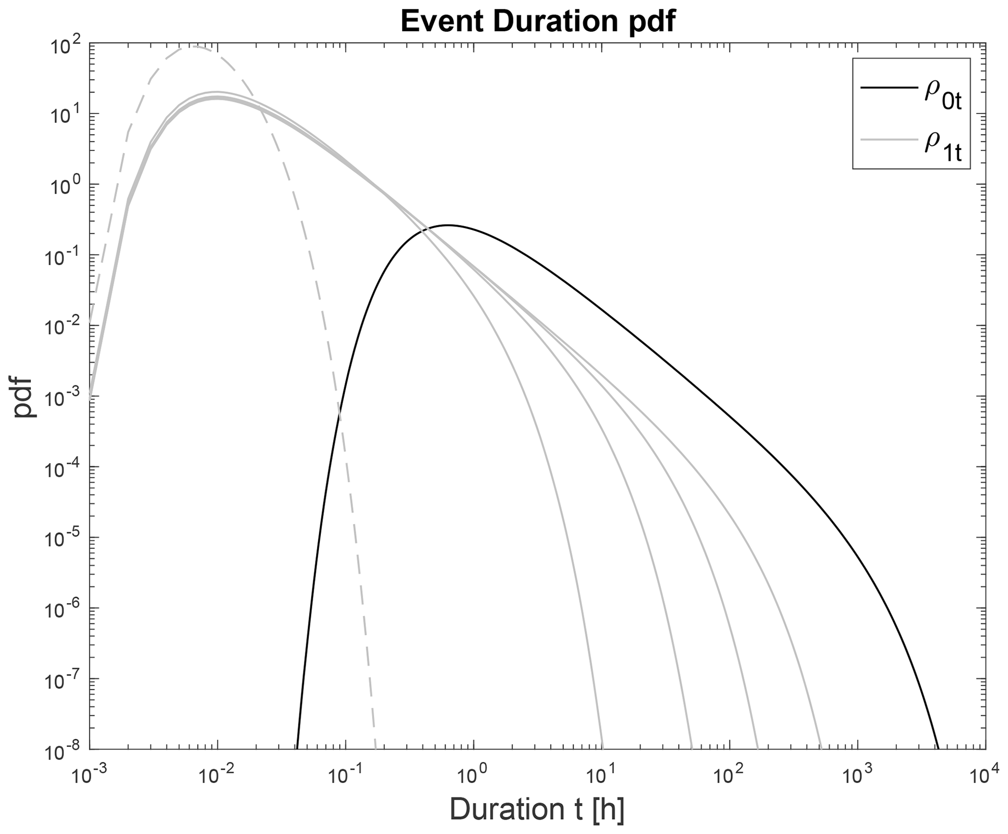
Figure 4Event duration pdfs for dry events (ρ0t black line) and rain events (ρ1t gray lines) for and 0.1. The dashed line is for ϵ=0.01.
4.3 Average cloudiness
The average cloudiness is the fraction of time that the stationary process is in the rain state σ>0. It is defined as
where is the solution to the steady-state Fokker–Planck Eq. (23). For the process σϵ, it is
Furthermore, the variance of the average cloudiness is
The average cloudiness is zero when using the point-process model σ. However, for σϵ as ϵ tends to zero, the average cloudiness and its variance are O(ϵ) and nonzero.
4.4 Total rainfall
For an example of using the results of Theorem 2, consider calculating the total rainfall at a specific grid point of a global circulation model. Define the rainfall time series at a point as
where σ encodes the rainfall rate, and ϕ(t)=1 when there is a cloud (or rainfall) and ϕ(t)=1 otherwise. One question is what the impact is on total rainfall in a simulation of time T between the rain processes σϵ and σ.
Theorem 2 states that the integrated difference of the total rainfall tends to zero. That is,
The proof of the theorem in the Appendix yields more information than that. For example, if it is known that there are N rain events after time T, then estimate Eq. (A45) yields
where the probability of N events is one and where the final remainder term has been dropped (for clarity of this calculation). Here K is a global bound on the function ϕ. For this example, K=1. From the estimates in the proof, the right-hand side is bounded by terms which have the first four moments of the event duration time τr,ϵ, the global bound K of ϕ, and the number of rain events. Thus, Theorem 2 and its proof give details on the differences for key atmospheric elements when using the rain processes σϵ and σ.
4.5 Modifications for the point-process model
The issue of how to use a finite-event-duration model to inform parameter selection is discussed in this subsection. There are two potential points of concern with the point-process model. One is that the point-process model σ(t) has rain events of duration zero, whereas the rain process model σϵ(t) has rain events of duration Thus, for time T,
where 𝒩(T) is the random number of rain events in T time. For finite ϵ>0 the value of 𝒩(T) is larger than for the point-process model, on average.
There are many potential solutions for the issue of zero-event times for the point-process model. One example is to modify the dry-duration pdf to account for the small but finite size of rain events. That is, let τr be a random variable which models a finite-size rain event. For example, see Eq. (28). Define
as a new dry event random variable. This new event distribution would account for the rain event within the dry event. As for the moisture process q, once the threshold of q=b is met, the process then holds at b for a random time of τr. Then the process would jump to q=0.
Another potential modification is the definition of rain amount. For the model with finite ϵ>0, for each event the model rains b amount over a random time τr,ϵ. For the point-process model, the model rains b amount instantaneously. Here the discrepancy between the two models is captured in Theorem 2, and the example of total rainfall is the example in Sect. 4.4. A possible modification to the model would be to use a finite-event-duration model to help assign a random magnitude to each point-process model event. For example, let bi be random variables with some distribution from a finite-event-duration model which accounts for random rain amounts. Then the point-process model can be modified from Eq. (7) as
In this paper, a threshold model for moisture and rain was shown to converge to a point process and related processes and to converge for various modes of convergence. By demonstrating this type of convergence, the simple ideas of a point-process model of rainfall, which at first may appear to be only an empirical model, can be linked with underlying physical processes and the evolution of moisture.
Here convergence for the moisture processes was defined and shown for the Fokker–Planck equation as well as the paths of the processes. Furthermore, the convergence of the rain process was shown in mean square difference with respect to the space of generalized functions.
Using a point process to approximate rainfall allows simplification for computation and exact formulas. For example, the autocorrelation function is known in the case of point processes as shown in Abbott et al. (2016). Furthermore, point processes have been studied extensively in the neural science literature (Sacerdote and Giraudo, 2013), and many statistics have been derived. Some examples of exact statistics are shown. These examples have interesting characteristics as the small parameter ϵ tends to zero.
The proofs shown here are revealing on their own, and they demonstrate further details of the convergence. The Fokker–Planck derivation in Sect. 3.1 shows that the density for the moisture in the rain state tends to zero, while the flux term remains nonzero, allowing for the “teleporting” boundary condition that arises for the limiting moisture process. For the convergence of paths of moisture shown in Theorem 1, the moisture process must first be decoupled into a moistening and precipitating process. Then the moistening process is shown to converge (Theorem 1), while the precipitating process contains all of the discontinuities. Finally, the proof of convergence of the rain processes in Theorem 2 gives estimates that would be useful for determining the error rates for using the point-process approximation. This is done in an example of total rainfall.
The rigorous mathematical proofs and formal asymptotic analysis for the results presented in Sect. 3 are given in this Appendix.
A1 Derivation of the Fokker–Planck equation
The Fokker–Planck equation for the process qϵ is
To derive the limiting (ϵ→0) Fokker–Planck equation, the analysis follows the procedure of matched asymptotic expansions (see, e.g., Bender and Orszag, 2013). Consider two regions [0,ϵ] and [ϵ,∞). Let ρ1,B be the density in the first region, which is a boundary layer region, and let ρ1,A be the density away from this region. Since the Fokker–Planck equations have parameter ϵ, let ρ1,B have the asymptotic expansion of the form
and let ρ1,A have the asymptotic expansion
These expansions are stopped at the order ϵ level. This is due to the higher-order terms not having an impact on the limiting equation. In the end, it will be shown that For the region away from the boundary, the density is This allows for the teleporting boundary condition of f0(b,t)δ(q).
First, to show , consider Eq. (A2) with the rescaled variable . This yields the equation
Substituting this expansion into Eq. (A3) yields, at order ϵ−2 and order ϵ−1, respectively,
Note that the O(1) equation is not written. At this order and higher, there are iterative PDEs written for for i≥2. These terms will converge to zero at a rate O(ϵi) and thus are not considered here. By solving the order ϵ−2 equation in Eq. (A4a) and applying the absorbing boundary condition at , one arrives at
The order ϵ−1 equation in Eq. (A4b) has essentially the same solution as above, and, after applying the absorbing boundary condition, one finds
Now consider the interval away from the boundary [ϵ,∞). Let ρ1,A be the density in this region. The equation in this region is
Note that the δ term acts on f0, which is a function of ρ0. The asymptotic expansion is for ρ1 only in the [ϵ,∞) region, and thus the density ρ0 is a first-order term. Substituting the expansion into Eq. (A7) gives the following equations, separated into their orders of ϵ:
The order ϵ−1 equation in Eq. (A8a) has the solution
Note that ρ1,A is a density, and thus must be integrable on [O(ϵ),∞). Thus, C3(t)=0 and
From the first-order equation in Eq. (A8b), by substituting in , we arrive at
Note that the constant of integration in each interval of b must be the same. Otherwise, the magnitude of the δ function in Eq. (A8b) would not be correct. The density must be integrable, which implies that
It is assumed that the matching between the A and B solutions must occur at an intermediate location or overlapping region. That is, for values of ,
and
The first equation implies that C1(t)=0 and . In the limit as ϵ→0, the second equation yields
Thus, the densities are
and
Note that the flux of ρ1 at q=0 is, to leading order, in terms of ,
Using the asymptotic formula for yields
Consequently, while the rain-state density itself is small (i.e., ), the flux f1 of the rain state is O(1), and its value f1(0,t) at the threshold q=0 represents an O(1) flux from the rain state to the dry state.
Thus, the Fokker–Planck-type equation for q(t) is
with the following conditions:
A2 Proof of Lemma 1
Note that the process 𝒩ϵ(T) is a renewal process. It is defined by the interarrival times
where is the duration for the ith dry (rain) event of the σϵ process. Note that Sn is used instead of to align with the common notation of renewal processes. The distributions of and are the same and are independent of ϵ, while depends on ϵ. For the lemma, the quantity of interest is the probability of having N rain events in time T, which is defined as
The probability on the right-hand side is estimated crudely by only considering one of the two events. Note that are independent and identically distributed (IID) random variables with , and , so that
The above probability is estimated by using a variant of the Chernoff bound (Hoeffding, 1994). That is,
for any s>0, where is the moment-generating function for the random variable Si. The moment-generating function can be factored due to independence of and :
These moment-generating functions are computed explicitly from the distributions found in Hottovy and Stechmann (2015b). They are
which are defined for . Chernoff's bound then yields
□
A3 Proof of Theorem 1
To begin, note that the SDEs for Eϵ and E (see Eq. 8) only differ when . Thus, the solutions to the SDEs give the formula
where 𝒩ϵ(T) is the number of rain events for T<∞, and ϵ>0 is fixed. Note that interval has been written as to emphasize the rain event duration . To proceed, the number of rain events is conditioned to be N. Note that m>0 and the stochastic integral is a martingale, and Doob's maximal inequality yields
By Lemma 1, the sum above converges due to the fast decay of P(𝒩ϵ(T)=N) as N→∞. Applying the Cauchy–Schwarz inequality to the sum and the Itô isometry to the stochastic integral yields
where τr,ϵ denotes the general event duration, which has the same distribution as all of the IID . This sum converges due to the fast decay of P(𝒩ϵ(T)=N) as shown in Eq. (A32).
To finish the proof, the following moments of are used. The integrals can be computed exactly using the densities for found in Hottovy and Stechmann (2015b). They are
Thus, the limit is
where Tonelli's theorem allows the limit as ϵ→0 to exchange with the infinite sum. This completes the proof.
□
A4 Proof of Theorem 2
To prove the theorem, the expectation is conditioned on the number of events 𝒩ϵ(T), as was done in the previous section. Thus, the expectation is
where 𝒩(T) is the number of dry events for the σ(t) process up to time T. Again, because of the decay of P(𝒩ϵ(T)=N) as N→∞ given in Lemma 1, the infinite sum converges.
To estimate the quantity in Eq. (A40), one rain event is considered, and the Cauchy–Schwarz bound will be used. Consider the ith rain event:
The function ϕ(t) is smooth on [0,T] and thus is locally Lipschitz. Let the Lipschitz constant be K>0. Then, along with the triangle inequality,
where the last inequality results from being an increasing function on . Using the inequality above, along with the Cauchy–Schwarz inequality, the quantity in Eq. (A40) is bounded by
where all expectations are conditional on 𝒩ϵ(T)=N.
To finish the theorem, the following moments of are used:
Thus, the first term in Eq. (A45) is
The second term in Eq. (A45) is
where the expectation turns into a product because and are independent. For the third term of Eq. (A45), the Lipschitz condition is used to write
Note that the stopping times can be written in terms of the moistening processes in the following way:
where . Similarly,
where the Wiener process is the same realization as in Eq. (A57). The definitions of the stopping times 𝒯2i−1 and 𝒯i imply
Thus, the difference in stopping times is
where the triangle inequality has been used. Taking the expected value and using the Itô isometry yields
Note that and are IID random variables with the same distribution, and thus the expectations cancel. For the remaining terms, the moments of in Eq. (A46) are used to give
which completes the consideration of the third term of Eq. (A45).
For the last “remainder” term in Eq. (A45), the expectation is conditioned on both 𝒩(T) and 𝒩ϵ(T). That is,
If 𝒩ϵ(T)≥𝒩(T), then there is no sum, and the term is zero. If 𝒩ϵ(T)≠𝒩(T), then the processes and Et from Sect. 3.3 must be at least b units apart. Thus, by Theorem 1,
Furthermore, convergence in expectation (L2) implies convergence in probability. Therefore,
Putting this together with the above estimate yields
by using Tonelli's theorem to exchange the sums and the limit. Thus, all of the terms in Eq. (A45) have been shown to converge to 0 as ϵ→0, so that, returning to Eq. (A40) and taking the limit, we have
and the proof is completed.
□
Code to produce the figures is available from the authors on request.
All of the data used in this paper are publicly available from the references listed.
Both the authors contributed to the final draft of the work. Additionally, SH contributed to the formal analysis and writing of the original draft preparation, and SNS contributed to the conceptualization and writing, review, and editing.
The contact author has declared that neither of the authors has any competing interests.
Publisher's note: Copernicus Publications remains neutral with regard to jurisdictional claims in published maps and institutional affiliations.
This research has been supported by the Division of Mathematical Sciences (grant no. 1815061).
This paper was edited by Balasubramanya Nadiga and reviewed by three anonymous referees.
Abbott, T. H., Stechmann, S. N., and Neelin, J. D.: Long temporal autocorrelations in tropical precipitation data and spike train prototypes, Geophys. Res. Lett., 43, 11–472, 2016. a, b, c, d
Ahmed, F. and Neelin, J. D.: Explaining scales and statistics of tropical precipitation clusters with a stochastic model, J. Atmos. Sci., 76, 3063–3087, 2019. a
Albano, G., Giorno, V., Nobile, A. G., and Ricciardi, L. M.: Modeling refractoriness for stochastically driven single neurons, Scientiae Mathematicae Japonicae, 67, 173–190, 2008. a
Bender, C. M. and Orszag, S. A.: Advanced mathematical methods for scientists and engineers I: Asymptotic methods and perturbation theory, Springer Science & Business Media, ISBN 0387989315, 2013. a, b
Bhat, V. N.: Renewal approximations of the switched Poisson processes and their applications to queueing systems, J. Oper. Res. Soc., 45, 345–353, 1994. a
Cowpertwait, P., O'Connell, P., Metcalfe, A., and Mawdsley, J.: Stochastic point process modelling of rainfall. I. Single-site fitting and validation, J. Hydrol., 175, 17–46, 1996. a
Cox, D. R.: Renewal theory, Methuen, London, ISBN 978-0412205705, 1962. a
Deluca, A. and Corral, Á.: Scale invariant events and dry spells for medium-resolution local rain data, Nonlin. Processes Geophys., 21, 555–567, https://doi.org/10.5194/npg-21-555-2014, 2014. a
Deluca, A., Moloney, N. R., and Corral, Á.: Data-driven prediction of thresholded time series of rainfall and self-organized criticality models, Phys. Rev. E, 91, 052808, https://doi.org/10.1103/PhysRevE.91.052808, 2015. a
Evans, M. R. and Majumdar, S. N.: Diffusion with stochastic resetting, Phys. Rev. Lett., 106, 160601, https://doi.org/10.1103/PhysRevLett.106.160601, 2011. a
Evans, M. R., Majumdar, S. N., and Schehr, G.: Stochastic resetting and applications, J. Phys. A., 53, 193001, https://doi.org/10.1088/1751-8121/ab7cfe, 2020. a
Filippov, A. F.: Differential equations with discontinuous righthand sides: control systems, vol. 18, Springer Science & Business Media, ISBN 9789027726995, 2013. a
Foufoula-Georgiou, E. and Lettenmaier, D. P.: A Markov renewal model for rainfall occurrences, Water Resour. Res., 23, 875–884, 1987. a
Frierson, D. M. W., Majda, A. J., and Pauluis, O. M.: Large scale dynamics of precipitation fronts in the tropical atmosphere: a novel relaxation limit, Commun. Math. Sci., 2, 591–626, 2004. a
Gardiner, C. W.: Handbook of stochastic methods: for physics, chemistry & the natural sciences, vol. 13 of Springer Series in Synergetics, Springer–Verlag, Berlin, ISBN 9783540707127, 2004. a, b, c
Green, J. R.: A model for rainfall occurrence, J. Roy. Stat. Soc. Ser. B, 26, 345–353, 1964. a
Hernandez-Duenas, G., Smith, L. M., and Stechmann, S. N.: Weak-and strong-friction limits of parcel models: Comparisons and stochastic convective initiation time, Q. J. Roy. Meteor. Soc., 145, 2272–2291, https://doi.org/10.1002/qj.3557, 2019. a
Hoeffding, W.: Probability inequalities for sums of bounded random variables, in: The Collected Works of Wassily Hoeffding, Springer, 409–426, ISBN 9780387943107, 1994. a
Holloway, C. E. and Neelin, J. D.: Temporal relations of column water vapor and tropical precipitation, J. Atmos. Sci., 67, 1091–1105, 2010. a
Hottovy, S. A. and Stechmann, S. N.: A spatiotemporal stochastic model for tropical precipitation and water vapor dynamics, J. Atmos. Sci., 72, 4721–4738, https://doi.org/10.1175/JAS-D-15-0119.1, 2015a. a, b
Hottovy, S. A. and Stechmann, S. N.: Threshold models for rainfall and convection: Deterministic versus stochastic triggers, SIAM J. Appl. Math., 75, 861–884, https://doi.org/10.1137/140980788, 2015b. a, b, c, d, e
Huang, T., Stechmann, S. N., and Torchinsky, J. L.: Framework for idealized climate simulations with spatiotemporal stochastic clouds and planetary-scale circulations, Phys. Rev. Fluids, 7, 010502, 2022. a
Jakubowski, A.: A non-Skorohod topology on the Skorohod space, Electron. J. Probab., 2, 1–21, https://doi.org/10.1214/EJP.v2-18, 1997. a
Katz, R. W.: Precipitation as a chain-dependent process, J. Appl. Meteorol., 16, 671–676, 1977. a
Kelley, J. L.: General topology, Courier Dover Publications, ISBN 9783540901259, 2017. a, b
Khouider, B. and Majda, A. J.: A non-oscillatory balanced scheme for an idealized tropical climate model: Part I: Algorithm and validation, Theor. Comp. Fluid Dyn., 19, 331–354, 2005. a
Khouider, B., Biello, J. A., and Majda, A. J.: A stochastic multicloud model for tropical convection, Comm. Math. Sci., 8, 187–216, 2010. a
Kurtz, T. G.: Random time changes and convergence in distribution under the Meyer-Zheng conditions, Ann. Probab., 19, 1010–1034, 1991. a
Lejay, A. and Pigato, P.: A threshold model for local volatility: evidence of leverage and mean reversion effects on historical data, Int. J. Theor. Appl. Finan., 22, 1950017, https://doi.org/10.1142/S0219024919500171, 2019. a
Lin, J. and Neelin, J.: Influence of a stochastic moist convective parameterization on tropical climate variability, Geophys. Res. Lett., 27, 3691–3694, https://doi.org/10.1029/2000GL011964, 2000. a
Mueller, E. A. and Stechmann, S. N.: Shallow-cloud impact on climate and uncertainty: A simple stochastic model, Mathematics of Climate and Weather Forecasting, 6, 16–37, 2020. a
Neelin, J. D., Sahany, S., Stechmann, S. N., and Bernstein, D. N.: Global warming precipitation accumulation increases above the current-c limate cutoff scale, P. Natl. Acad. Sci. USA, 114, 1258–1263, https://doi.org/10.1073/pnas.1615333114, 2017. a
Peters, O. and Neelin, J. D.: Critical phenomena in atmospheric precipitation, Nat. Phys., 2, 393–396, 2006. a
Peters, O., Deluca, A., Corral, A., Neelin, J. D., and Holloway, C. E.: Universality of rain event size distributions, J. Stat. Mech., 2010, P11030, https://doi.org/10.1088/1742-5468/2010/11/P11030, 2010. a
Richardson, C. W.: Stochastic simulation of daily precipitation, temperature, and solar radiation, Water Resour. Res., 17, 182–190, 1981. a
Rodriguez-Iturbe, I., Cox, D. R., and Isham, V.: A point process model for rainfall: further developments, P. Roy. Soc. Lond. A Mat., 417, 283–298, 1988. a
Sacerdote, L. and Giraudo, M. T.: Stochastic integrate and fire models: a review on mathematical methods and their applications, in: Stochastic biomathematical models, Springer, 99–148, https://doi.org/10.1007/978-3-642-32157-3_5, 2013. a, b
Simpson, D. J. W. and Kuske, R.: Stochastically perturbed sliding motion in piecewise-smooth systems, arXiv [preprint], https://doi.org/10.48550/arXiv.1204.5792, 2012. a
Smith, J. A. and Karr, A. F.: A point process model of summer season rainfall occurrences, Water Resour. Res., 19, 95–103, 1983. a
Stechmann, S. N. and Hottovy, S.: Cloud regimes as phase transitions, Geophys. Res. Lett., 43, 6579–6587, 2016. a
Stechmann, S. N. and Neelin, J. D.: A stochastic model for the transition to strong convection, J. Atmos. Sci., 68, 2955–2970, 2011. a
Stechmann, S. N. and Neelin, J. D.: First-passage-time prototypes for precipitation statistics, J. Atmos. Sci., 71, 3269–3291, 2014. a, b
Whitt, W.: Approximating a point process by a renewal process, I: Two basic methods, Oper. Res., 30, 125–147, 1982. a
Wilks, D. S. and Wilby, R. L.: The weather generation game: a review of stochastic weather models, Prog. Phys. Geog., 23, 329–357, 1999. a