On the interaction of stochastic forcing and regime dynamics

Stochastic forcing can, sometimes, stabilise atmospheric regime dynamics, increasing their persistence. This counter-intuitive effect has been observed in geophysical models of varying complexity, and here we investigate the mechanisms underlying stochastic regime dynamics in a conceptual model. We use a six-mode truncation of a barotropic β-plane model, featuring transitions between analogues of zonal and blocked flow conditions, and identify mechanisms similar to those seen previously in work on low-dimensional random maps. Namely, we show that a geometric mechanism, here relating to monotonic instability growth, allows for asymmetric action of symmetric perturbations on regime lifetime and that random scattering can “trap” the flow in more stable regions of phase space. We comment on the implications for understanding more complex atmospheric systems.

1 Introduction

Rossby (1940) first suggested the atmosphere may possess multiple large-scale quasi-equilibrium states to describe the empirically observed tendency for European weather patterns to take on a finite range of frequently recurrent configurations. These are now known in meteorology as atmospheric regimes, and in dynamical systems, such behaviour is known as crisis-induced intermittency (Ott, 2002). The first theoretical study of multiple atmospheric equilibria, carried out by Charney and DeVore (1979) (hereafter CdV79), showed that the flow in a low-order mid-latitude barotropic channel could equilibrate to either a zonally symmetric flow or a stationary blocking pattern. They suggested real-world equivalents of these equilibria states might be destabilised by perturbations from unresolved modes (in this idealised model, this included spatial scales of ∼𝒪(1000) km), causing shifts from one state to another and introducing a vacillation between large-scale weather patterns.

Similar results were obtained in other simple models (Charney and Straus, 1980; Kallen, 1981; De Swart, 1988), but these equilibria were often absent in less truncated systems, rendered “unrealisable” by shifts in the model attractor or collapsing completely due to structural instability (Reinhold and Pierrehumbert, 1982; Cehelsky and Tung, 1987). Therefore later work moved away from analysis of fixed points, treating regimes as chaotic flows originating from attractor merging (Itoh and Kimoto, 1996, 1997) and exploring the role of homoclinic orbits in preferred transitions between regimes (Kimoto and Ghil, 1993; Kondrashov et al., 2004; Selten and Branstator, 2004).

Despite a deepening mathematical understanding of regimes, the Earth system appears to be high-dimensional, and as a result linking the regime behaviour of simple models to that of realistic models has proved challenging, especially when further complicated by the introduction of stochastic forcing. Earth-system models often contain explicit stochastic parameterisation schemes and in addition a range of small-scale processes that can be thought of as randomly forcing the large-scale flow. Contrary to linear intuition, there is evidence that this fast variability can stabilise regimes: Kwasniok (2014) (hereafter K14) found additive noise increases regime lifetime in both the Lorenz 1963 system (Lorenz, 1963) and a chaotic reformulation of the CdV79 model found by Crommelin et al. (2004) (hereafter C04). Further, stochastic forcing has been shown to improve regime predictability by increasing persistence in truncations of the Lorenz 1996 model (Düben et al., 2014; Christensen et al., 2015) and climate model regime representation (Dawson and Palmer, 2015), as well as the representation of other slow-varying climate modes (Palmer and Weisheimer, 2011; Berner et al., 2012).

Outside of geoscience, similar stochastic persistence effects have been observed and explained for transient chaotic maps. For such open systems, chaotic dynamics only persist for finite time, eventually “escaping”, often to a steady state (Lai and Tél, 2011a). It has been shown for such systems how stochastic forcing can delay the escape of trajectories in the case of 1D (Reimann, 1996; Lai and Tél, 2011b) and 2D (Altmann and Endler, 2010) maps via a “fattening” of the fractal structure. This is of interest for fully chaotic geophysical regime systems as the transition between regimes can be conceived of as an escape from one regime to another, and so increases in regime persistence correspond to decreases in escape rate. This approach was introduced in Franaszek and Fronzoni (1994) to understand the stochastically forced Duffing oscillator.

We will study the stochastically forced CdV79 model, as retuned by C04, and show that similar mechanisms explain stochastic persistence in this six-dimensional, continuous-time, non-hyperbolic regime system as in simpler transiently chaotic maps. We introduce the model and its regime structure in Sect. 2. We then discuss the impact of stochasticity on that regime structure in Sect. 3 and demonstrate that this can be understood as a result of the theory of hitting time problems in combination with a geometric mechanism. We summarise our results and discuss the implications for weather and climate in Sect. 4.

2 Model formulation

The deterministic Charney–deVore model is obtained by spectral truncation of a barotropic flow in a β-plane channel geometry. It can be expressed as a system of six ordinary differential equations, derived in full in Appendix A:

$$\begin{array}{}\text{(1)}& \begin{array}{rl}{\dot{x}}_{\mathrm{1}}=& -C(x_{\mathrm{1}}-x_{\mathrm{1}}^{*})+{\stackrel{\mathrm{̃}}{\mathit{\gamma }}}_{\mathrm{1}}{x}_{\mathrm{3}}\\ {\dot{x}}_{\mathrm{2}}=& -C{x}_{\mathrm{2}}+{\mathit{\beta }}_{\mathrm{1}}{x}_{\mathrm{3}}-{\mathit{\alpha }}_{\mathrm{1}}{x}_{\mathrm{1}}{x}_{\mathrm{3}}-{\mathit{\delta }}_{\mathrm{1}}{x}_{\mathrm{4}}{x}_{\mathrm{6}}\\ {\dot{x}}_{\mathrm{3}}=& -C{x}_{\mathrm{3}}-{\mathit{\beta }}_{\mathrm{1}}{x}_{\mathrm{2}}+{\mathit{\alpha }}_{\mathrm{1}}{x}_{\mathrm{1}}{x}_{\mathrm{2}}+{\mathit{\delta }}_{\mathrm{1}}{x}_{\mathrm{4}}{x}_{\mathrm{5}}-{\mathit{\gamma }}_{\mathrm{1}}{x}_{\mathrm{1}}\\ {\dot{x}}_{\mathrm{4}}=& -C(x_{\mathrm{4}}-x_{\mathrm{4}}^{*})+\mathit{ϵ}(x_{\mathrm{2}}{x}_{\mathrm{6}}-x_{\mathrm{3}}{x}_{\mathrm{5}})+{\stackrel{\mathrm{̃}}{\mathit{\gamma }}}_{\mathrm{2}}{x}_{\mathrm{6}}\\ {\dot{x}}_{\mathrm{5}}=& -C{x}_{\mathrm{5}}+{\mathit{\beta }}_{\mathrm{2}}{x}_{\mathrm{6}}-{\mathit{\alpha }}_{\mathrm{2}}{x}_{\mathrm{1}}{x}_{\mathrm{6}}-{\mathit{\delta }}_{\mathrm{2}}{x}_{\mathrm{4}}{x}_{\mathrm{3}}\\ {\dot{x}}_{\mathrm{6}}=& -C{x}_{\mathrm{6}}-{\mathit{\beta }}_{\mathrm{2}}{x}_{\mathrm{5}}+{\mathit{\alpha }}_{\mathrm{2}}{x}_{\mathrm{1}}{x}_{\mathrm{5}}+{\mathit{\delta }}_{\mathrm{2}}{x}_{\mathrm{4}}{x}_{\mathrm{2}}-{\mathit{\gamma }}_{\mathrm{2}}{x}_{\mathrm{4}}.\end{array}\end{array}$$

The six variables {x_i} represent spectral mode amplitudes of a streamfunction field, subject to a linear relaxation to a zonally symmetric background state, Coriolis and orographic forces, and quadratic advective non-linearities. To explore stochastic effects, we introduce an additive white noise vector to the tendency, given by a normal distribution ξ_i with standard deviation σ, as in K14:

$$\begin{array}{}\text{(2)}& {\dot{x}}_i={\dot{x}}_{i,\mathrm{deterministic}}+\mathit{\sigma }{\mathit{\xi }}_i.\end{array}$$

The system is integrated using the Euler–Maruyama difference scheme with a time step of $\mathrm{d}t=\mathrm{2}\times {\mathrm{10}}^{-\mathrm{4}}$ model time units (MTU) and is sampled every 1 MTU. We compute integrations of length 200 000 MTU for a range of σ values.

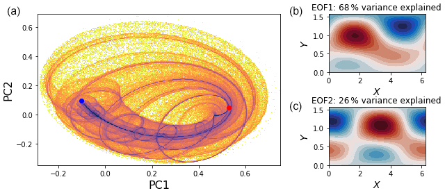
Figure 1 (a) Projection of the deterministic attractor into the space of the leading EOFs, capturing 92 % of the total variance. (b, c) The flow patterns corresponding to the first and second EOFs of the system. Blue and red dots show the positions of fixed points corresponding to blocked and zonal flows respectively.

Figure 2 A 2000 MTU integration of the CdV79 system, showing the evolution of each mode amplitude. The dynamics are chaotic but weakly so, showing clear quasi-periodic behaviour. Two regimes of behaviour can be seen: fast chaotic oscillations, divided by periods of slow evolution with irregular duration. The mode values at the blocked and zonal fixed points are shown with dashed blue and red lines.

To visualise the model phase space, we project the six-dimensional attractor into the space of the two leading empirical orthogonal functions (EOFs) of the deterministic system, as shown in Fig. 1, capturing 94 % of the system's variability (Fig. S1 in the Supplement shows the various projections of the six x modes). The attractor is highly structured, with a number of strongly preferred trajectories through phase space (note the logarithmic colour scheme in Fig. 1). This low-dimensional attractor shows no obviously separable phase space regions such as the twin lobes of the Lorenz 1963 system, and we see that the trajectories are highly twisted together, producing a scroll-like geometry.

A representative sample of the model's temporal evolution is shown in Fig. 2. Intermittency is readily apparent, with predictable slowly evolving periods, with near-zero phase speed, corresponding to persistent “blocked” flow patterns, divided by highly chaotic, fast-evolving flows that contain both zonally symmetric states and transient wave activity. The regime structure is therefore quite asymmetrical, in contrast to the Lorenz 1963 or 1996 systems whose regimes are essentially equivalent to each other. Instabilities in the CdV system arise from two basic mechanisms: an orographically induced saddle-node bifurcation (a transition from one to multiple fixed-point equilibria), as identified in the original CdV79 paper, and a barotropic Hopf bifurcation (a transition from a fixed point to a periodic orbit) associated with the onset of a zonally propagating waves in the model domain. Both bifurcations are codimension 1, existing along a surface with one fewer dimension than the parameter space, and so can in general be found by tuning one model parameter. Stable steady-state and periodic wave solutions to Eq. (1) are common for arbitrary sets of model parameters (not shown), while chaotic – and especially intermittently chaotic – solutions are harder to find. In the original formulation of CdV79, two stable fixed points were found, corresponding to a zonally symmetric state, and a “blocked” flow, with strong wave activity. The model parameters used here, and in C04 and K14, are close to a parameter set where the barotropic Hopf and orographic saddle-node bifurcations merge: one fixed point bifurcates into two fixed points and a limit cycle. This fold-Hopf point has codimension 2, meaning two model parameters must be tuned to obtain it. High-codimension bifurcations seem to be of reduced relevance to the real world, representing exceptional states in parameter space. However, the fold-Hopf bifurcation is known to produce a range of lower codimension and so more relevant bifurcations at nearby parameter values, including paths to chaotic dynamics (Champneys and Kirk, 2004). Most relevant to us is the generation of homoclinic orbits, a type of bifurcation where orbits stretch from a fixed point back to itself, with an infinite period. These orbits can lead to fully fledged chaotic dynamics and the creation of a strange attractor through intersection with an unstable toroidal limit cycle. At the boundary crisis this creates a “whirlpool repeller” (Shilnikov et al., 1995) and exactly the scrolling structure seen in Fig. 1. The two fixed points, analogues of those in CdV79, remain but are now unstable, and at the parameter values chosen here the strange attractor moves between the vicinity of these two fixed points, as seen in Figs. 1 and 2, shadowing collapsed homoclinic orbits. The flow patterns corresponding to these fixed points are shown in Fig. S2. See De Swart (1988) and C04 for more details on the bifurcation structure of the model. As a result the regimes of the CdV system are rooted in the dynamics of unstable homoclinic orbits, with close approaches to the unstable fixed point leading to periods of slow evolution and then rapid “bursting” to chaotic, more turbulent flow. Such behaviour is seen in other simple atmospheric models (Crommelin, 2002) including the Lorenz 1984 model (Shilnikov et al., 1995) and in the dynamics of non-linear circuits (Pusuluri and Shilnikov, 2018) and neurons (Izhikevich, 2006).

This type of regime behaviour is of a fundamentally different type to that of the archetypal Lorenz 1963 system. In Lorenz 1963, crisis-induced intermittency creates regime dynamics when the basins of attraction of two attractors merge together, triggering movement between two distinct regimes of fully chaotic behaviour. The Charney–deVore system, in contrast, experiences almost deterministic dynamics before drifting away and entering a transient chaotic regime. At an unpredictable later time, the system will once again return to the neighbourhood of the periodic orbit and re-enter the slow-evolving regime. For a recent discussion of the co-existence of predictable and chaotic flow states in atmospheric systems see Shen et al. (2021).

Regimes in CdV

When studying a multimodal system, bulk metrics such as the mean or variance can obscure the underlying dynamical structure. Therefore it is natural to use a regime framework as a way of partitioning phase space into dynamically distinct regions of interest. Following the approach of K14, we use a hidden Markov model (HMM) to identify qualitatively different dynamical regimes, with the minor methodological change of fitting the HMM to the full six-dimensional state vector, rather than restricting it to the x₁–x₄ subspace as in K14. As for most clustering methods, we must make a subjective choice of regime number when fitting the HMM. We use three regimes, which were found in K14 to separate the qualitatively distinct model dynamics well, capturing both the persistent quasi-predictable blocking regime and the highly chaotic zonal regime and the transitions between them. Figure 3a shows the regions of the deterministic attractor assigned to each regime, and Fig. S3 shows the corresponding flow patterns. The blocking regime is small in phase space extent, focused on the tightly spiralled trajectories that start close to the blocking fixed point. It clearly separates from the swirling trajectories assigned to the transitional regime. The zonal state contains the very chaotic “branching” of the attractor into different orbits and contains the early parts of these orbits until their transition back to blocking becomes unavoidable. Interestingly, these regimes broadly correspond to regions of the attractor with different numbers of unstable dimensions (Fig. 3b), supporting our choice of three regimes as dynamically appropriate. Our regime assignment also has some similarities to the regimes found in Strommen et al. (2022), which used persistent homology to identify regimes in the system studied here and found a persistent component similar to our blocking state.

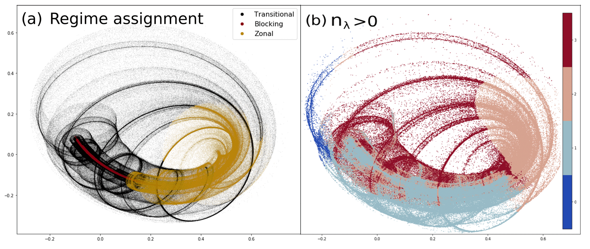
Figure 3 (a) The assignment of points on the deterministic model attractor to the three hidden Markov model regimes projected into the EOF1–EOF2 plane. (b) The number of unstable dimensions as identified by the positive local Lyapunov exponents, calculated at each point along the deterministic model attractor, projected into the EOF1–EOF2 plane.

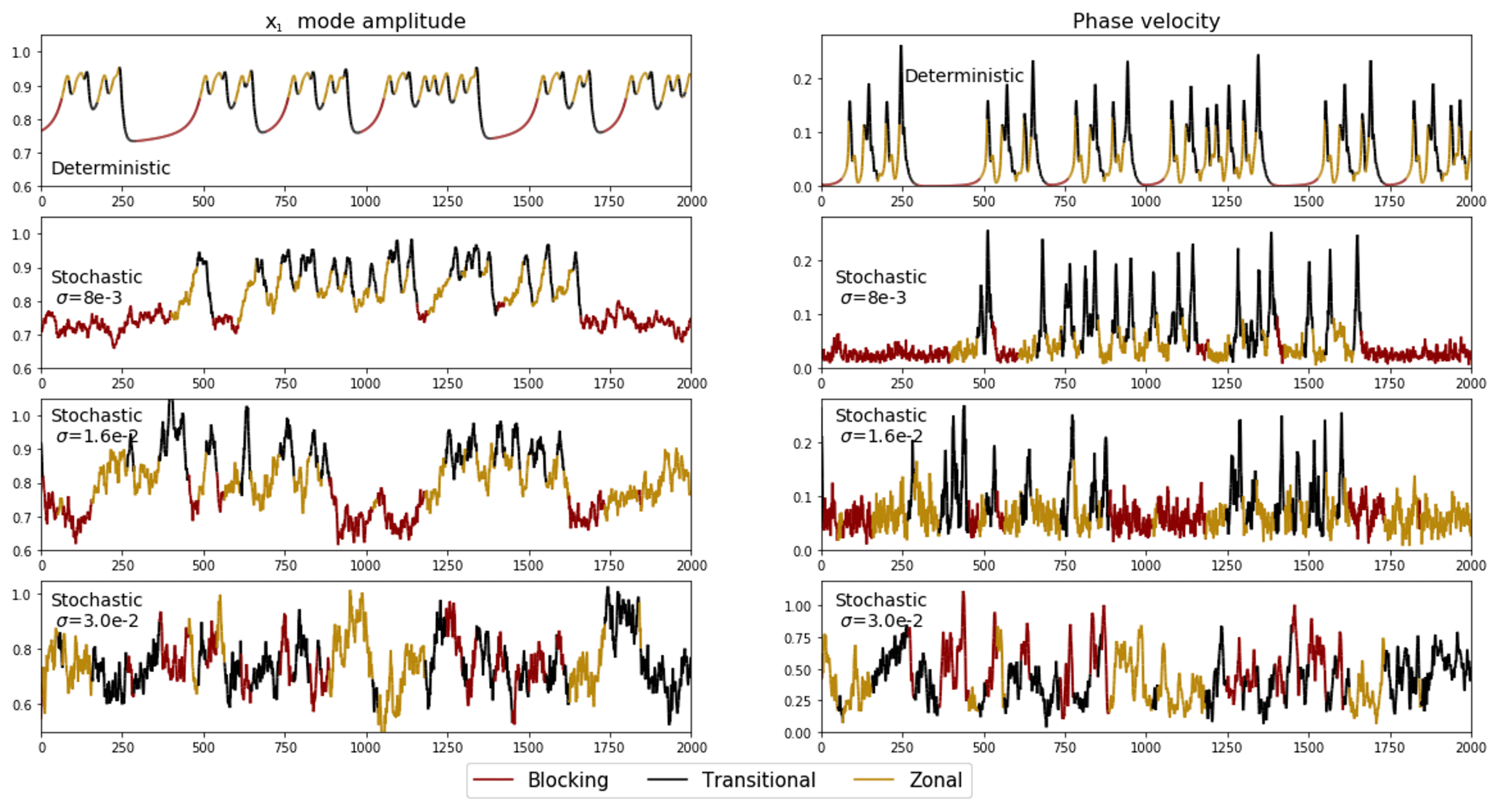
Figure 4 Left: time evolution of the x₁ mode in deterministic and stochastic cases, with points coloured by their regime assignment. Right: the corresponding phase velocities.

For non-zero noise amplitude, σ≠0, we identify regimes in the same way, refitting the HMM for each σ value. This is necessary as while the qualitative shape of the attractor¹ is robust over a range of noise amplitudes, the fine structure seen in Fig. 1 breaks down, and the stochastic simulations experience shifts of probability density closer to the location of the blocking fixed point (shown in Fig. S4).

Figure 4 shows the temporal evolution of the zonally symmetric x₁ mode, and the phase velocity $v_t=\frac{\mathrm{1}}{\mathrm{2}}\sqrt{{\sum }_{i=\mathrm{1}}^{\mathrm{6}}(x_{i,t+\mathrm{1}}-x_{i,t-\mathrm{1}}{)}^{\mathrm{2}}}$, for different σ values, coloured by regime assignment. The characteristics of the regimes are broadly preserved even up to $\mathit{\sigma }=\mathrm{1.6}\times {\mathrm{10}}^{-\mathrm{2}}$: the persistent blocking state has low x₁ values and very low phase velocities, and the zonal state has high x₁ values and relatively low phase velocities, while the transitional regime has high x₁ values and high phase velocity. However, for the larger value of $\mathit{\sigma }=\mathrm{3.0}\times {\mathrm{10}}^{-\mathrm{2}}$, it is apparent that there is no meaningful regime structure remaining: the phase velocity never drops below 0.2, indicating a loss of quasi-stationarity. At this point the deterministic dynamics play second fiddle to the stochastic term, and the assignment of regimes becomes meaningless.

3 Stochastic persistence

Figure 5a shows Fourier transforms of the total mode amplitude $\sqrt{{\sum }_i{x}_i^{\mathrm{2}}}$ for three representative amplitudes of stochastic forcing. The deterministic σ=0 spectrum possesses a clear peak consistent with the quasi-periodic nature of the dynamics. For the σ=0.01 case this peak has collapsed, producing a flatter spectrum with power shifted towards low frequencies. This is not a monotonic effect: for σ=0.04, the total power in the low-frequency region decreases, and the spectrum flattens. Figure 5b shows this non-monotonicity clearly, with a peak in low-frequency variability close to σ=0.01.

Figure 5 (a) The power spectral density of the total mode amplitude, $\sqrt{{\sum }_i{x}_i^{\mathrm{2}}}$, for three different strengths of stochastic forcing, σ. (b) The spectral power averaged over frequencies from $\mathrm{1}/\mathrm{500}$ to $\mathrm{1}/\mathrm{10}\mathrm{000}$ MTU⁻¹ (corresponding to the shaded region of panel a) as a function of σ.

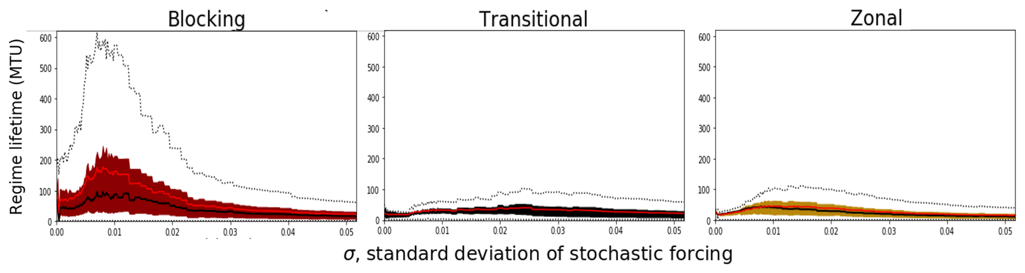
Figure 6 The distribution of blocking regime lifetimes, as a function of stochastic forcing amplitude. Shaded regions mark the interquartile range, with the thick black line showing the median and the red line the mean. Dotted black lines show the 0th and 95th percentiles of the distribution.

This is in excellent agreement with K14, which showed increasing regime persistence with noise amplitude that peaked at σ=0.008 and then decreased. We show here that this is associated with a genuine slowing of the system variables visible in the Fourier spectrum and is observable independent of adopting a regime perspective. With this reassurance, and given the HMM maintains the same qualitative characteristics for σ values ≤0.016, we judge that the regime assignment provides a sensible way to analyse the amplified low-frequency variability seen in Fig. 5 in more detail. Figure 6 shows the distribution of lifetimes for each of the three regimes, as a function of increasing σ. While all regimes show some increase in regime persistence for moderate noise amplitudes, the effect is by far the most significant in the blocking regime, showing a near trebling of mean regime lifetime that peaks at σ=0.008. As shown in Fig. S5, this peak is associated with a 150 % increase in the number of blocks lasting at least 100 MTU and a 600 % increase in those lasting longer than 175 MTU. Changes in the median blocking lifetime are smaller, and the distribution is clearly skewed, with the 95th percentile of blocking lifetime exceeding 600 MTU when persistence is maximum.

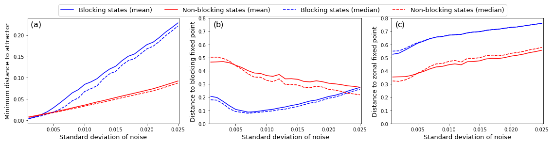
Figure 7 (a) The mean (solid lines) and median (dashed lines) Euclidean distance between points in the stochastic simulation and their closest neighbour on the deterministic attractor, shown for the blocking and non-blocking regimes. (b, c) As in (a) but showing the distance between points in each simulation and the blocking (b) and zonal (c) equilibria respectively.

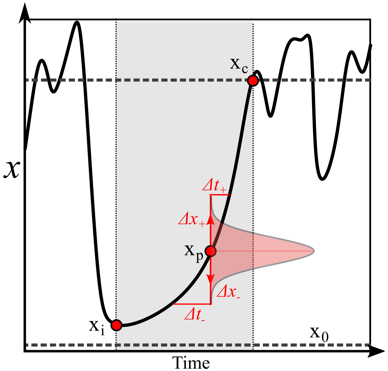
Figure 8 A schematic showing one variable, x, of a chaotic process, which moves between periods of chaotic variability and periods of predictable, monotonic growth (shaded in grey). The predictable regime is entered at a random position x_i, in the neighbourhood of an unstable fixed point x₀, and once it reaches an amplitude x_c, it will re-enter the chaotic regime. At a position x_p, we consider the impact of applying a random perturbation Δx to the x variable, drawn from some symmetric probability distribution, with vanishing support outside the interval [x₀−x_p,x_c−x_p]. We see that, due to the convex growth of x, a perturbation with negative sign will increase the duration of the predictable period more than a corresponding perturbation with positive sign will shorten it.

How can the ability of random forcing to stabilise regime dynamics be understood? What causes the non-monotonicity between stochastic amplitude and persistence, and why is the response here asymmetric, primarily in the blocking regime? As mentioned, non-monotonic changes of transient lifetime due to stochastic forcing are understood for low-dimensional transiently chaotic maps. Symmetric perturbations can decrease on average the region of phase space in which chaotic trajectories can “escape” (i.e. decay) for a large class of 1D concave maps, lengthening their lifetime (Reimann, 1996; Lai and Tél, 2011b). Additionally, stochasticity smooths the probability density of the deterministic system. If the escape region of the system is of higher than average density due to low dimensionality, then stochastic forcing can on average knock more trajectories out of this region than in to it, again increasing persistence (Altmann and Endler, 2010; Faisst and Eckhardt, 2003).

In our system we first consider the mean state changes. The average distance between points in the stochastic simulations and their closest neighbour on the deterministic attractor increases, approximately linearly, as the amplitude of the stochastic forcing increases (Fig. 7a). Once again there is asymmetry between regimes, with the minimum distance during blocking growing far faster than during the other regimes. Figure 7b and c show that this is associated with a drift towards the neighbourhood of the unstable blocking fixed point, with no equivalent result seen for the zonal fixed point (also visible in Fig. S4). If we consider the dynamics in the neighbourhood of the blocking fixed point, we realise the deterministic tendency there is near zero, and so the additive stochastic terms dominate entirely: the dynamics approach six-dimensional Brownian motion. How long, in expectation, will it take for this Brownian motion to move the system away from the fixed point once again and return it to a dynamics-dominated flow state? This question is simply a reformulation of the classic hitting time problem: at what time will a random process first reach a distance a from its initial condition? For Brownian motion in three or more dimensions it is known that in fact the average time taken is infinite: the distribution of hitting times is fat-tailed, and so the mean diverges (Kallenberg, 2017). Therefore the skewed distribution of blocking lifetimes seen in Fig. 6 can be understood in terms of the amount of time spent near the fixed point, as shown in Fig. 7b. As σ increases past 0.008, the average distance from both the attractor and the blocking fixed point increases. As the stochastic forcing becomes stronger than the deterministic damping along the stable manifold, the system increasingly explores the full six-dimensional phase space, and so the directionality of the forcing vanishes. There is a conceptual similarity here to the second stochastic persistence mechanism of Altmann and Endler (2010) found for mixed phase space systems, whereby trajectories in a 1D transiently chaotic map can scatter into islands of stability, which introduces a fat tail to the transient lifetime. However, the increased persistence we find is not entirely a result of excursions to the noise-dominated neighbourhood of the fixed point. There is also an important interaction between stochasticity and the low-dimensional, ordered flow of the blocking regime. We present a heuristic mechanism similar in character to that of Lai and Tél (2011b) but now considering a 1D flow as in the schematic shown in Fig. 8. We can think of this as a parameterisation along the 1D unstable manifold of our CdV79 system moving between a highly chaotic state and a slowly evolving, predictable state. Immediately upon entering the regime of slow-evolving dynamics, the system is at a point x=x_i and will stay in the quasi-stationary regime until it reaches x=x_c. We assume that x grows monotonically with the time t in this regime, so we can parameterise x in terms of t or vice versa: $f:x\to t$, $g:t\to x$. If we let x=f(t) be any convex, monotonic function defined over the interval [x₀,x_c], then $t=g\left(x\right)=f^{-\mathrm{1}}\left(x\right)$, and so g is therefore a concave, monotonic function with negative curvature. We consider applying a single perturbation Δx to the system at a point x_p, drawn from an even probability distribution P(Δx) with fast-decaying tails and support over [x₀−x_p, x_c−x_p]. Informally, this amounts to choosing a point x_p far from the edge of the predictable regime, and so there is only a vanishing probability of Δx directly triggering a regime transition. When the standard deviation of P is small compared to x_c−x₀, this will apply to most values of x in the interval. From the evenness of P, we see that the impact of the perturbation on the variable x, in expectation, is zero:

$$\begin{array}{}\text{(3)}& \langle \mathrm{\Delta }x\rangle =\mathrm{0}.\end{array}$$

However this is not in general the case for 〈Δt〉:

$$\begin{array}{}\text{(4)}& \langle \mathrm{\Delta }t\rangle =\langle g(x_{\mathrm{p}}+\mathrm{\Delta }x)-g\left(x_{\mathrm{p}}\right)\rangle =\langle G_p\left(\mathrm{\Delta }x\right)\rangle ,\end{array}$$

where G_p, as a translation of g, is also concave. Using the definition of the expectation we find

$$\begin{array}{}\text{(5)}& \langle \mathrm{\Delta }t\rangle =\underset{-\mathrm{\infty }}{\overset{\mathrm{\infty }}{\int }}{G}_p\left(\mathrm{\Delta }x\right)\cdot P\left(\mathrm{\Delta }x\right)\mathrm{d}\mathrm{\Delta }x,\end{array}$$

where the limits are justified by our requirement for vanishing tails for P and our choice of x_p.

Because P(Δx) is even, then if we Taylor-expand G_p, we will lose all odd powers on integration and be left with

$$\begin{array}{}\text{(6)}& \langle \mathrm{\Delta }t\rangle =\underset{-\mathrm{\infty }}{\overset{\mathrm{\infty }}{\int }}\sum _{n=\mathrm{1}}^{\mathrm{\infty }}{\displaystyle \frac{\mathrm{1}}{\left(\mathrm{2}n\right)\mathrm{!}}}{\displaystyle \frac{d^{\mathrm{2}n}{G}_p}{\mathrm{d}(\mathrm{\Delta }x{)}^{\mathrm{2}n}}}\cdot P\left(\mathrm{\Delta }x\right)\mathrm{d}\mathrm{\Delta }x.\end{array}$$

And having taken Δx to be small, we can drop high-order terms:

$$\begin{array}{}\text{(7)}& \langle \mathrm{\Delta }t\rangle =\underset{-\mathrm{\infty }}{\overset{\mathrm{\infty }}{\int }}{\displaystyle \frac{\mathrm{1}}{\mathrm{2}}}{\displaystyle \frac{d^{\mathrm{2}}{G}_p}{\mathrm{d}(\mathrm{\Delta }x{)}^{\mathrm{2}}}}\cdot P\left(\mathrm{\Delta }x\right)\mathrm{d}\mathrm{\Delta }x.\end{array}$$

Because G_p is concave, this derivative is negative, and we obtain

$$\begin{array}{}\text{(8)}& \langle \mathrm{\Delta }t\rangle =-\underset{-\mathrm{\infty }}{\overset{\mathrm{\infty }}{\int }}{\displaystyle \frac{\mathrm{1}}{\mathrm{2}}}\left|{\displaystyle \frac{d^{\mathrm{2}}{G}_p}{\mathrm{d}(\mathrm{\Delta }x{)}^{\mathrm{2}}}}\right|\cdot P\left(\mathrm{\Delta }x\right)\mathrm{d}\mathrm{\Delta }x=-I,\end{array}$$

where I is positive. Therefore any convex perturbation growth will be delayed (i.e. intermittency persisted) by small symmetric random perturbations, and the average lifetime of the stable regime will increase. The case for a negatively oriented variable with concave curvature is precisely equivalent, while for a positively oriented variable with concave curvature or a negatively oriented variable with convex curvature, decreased persistence would be seen. For the linear case with zero curvature, there is of course no impact of the perturbation on persistence.

When considering the particular case of f(t)=x₀e^λt, and $P\left(\mathrm{\Delta }x\right)=\mathcal{N}(\mathrm{0},\mathit{\sigma })$, which is interesting for our system, we obtain analytically $\langle \mathrm{\Delta }t\rangle =\frac{-{\mathit{\sigma }}^{\mathrm{2}}}{\mathrm{2}\mathit{\lambda }{x}_{\mathrm{p}}^{\mathrm{2}}}$ (see Appendix B). This quadratic dependence on σ² is exactly what is found in Lai and Tél (2011b) and Reimann (1996) for the escape rate for 1D maps. However it is not clear that the two derivations are totally equivalent; we consider a convex monotonic instability and they a concave non-invertible map. Higher σ corresponds to longer persistence (remembering our overall weak noise approximation), as does small λ, indicating that nearly stable intermittent dynamics can be most substantially persisted. We also see in this case that smaller x_p leads to larger drift, indicating that perturbations soon after the system has entered the intermittent state are most impactful. While we have considered only a single perturbation, the reasoning generalises to a continuous stochastic process, where the 〈Δt〉 term we have calculated is now a spatially dependent drift term. The crux of the argument can be understood solely from examination of Fig. 8. Any low-dimensional, convexly growing instability in the climate system should be susceptible to the same stochastic suppression. We can also see why only the blocking regime showed dramatic persistence increases, as it is the only regime where the variables evolve with a constant sign of curvature and where there is only one unstable dimension. The decrease of lifetime for larger noise values does not emerge naturally from this framework but can be understood as entering a noise-dominated regime where the stochastic terms are much larger than the deterministic tendency.

4 Conclusions

In this paper we have investigated the interaction between stochasticity and strongly non-linear dynamics in a six-equation conceptual model of atmospheric flow. We consider the case of additive stochastic forcing applied to a chaotic flow which transitions intermittently between chaotic zonal and quasi-stationary blocked regimes, which Kwasniok (2014) showed exhibited stochastically reinforced regime persistence for a range of noise amplitudes. We have investigated the mechanisms driving this behaviour and provide heuristic arguments based on the stochastic suppression of instability growth and random scattering close to an unstable fixed point. The low dimensionality and ordered nature of the blocking regime leads to a slow monotonically growing instability, which will on average be persisted by a random perturbation rather than accelerated. This effect is amplified, and a heavy tail introduced into the lifetime of blocking events, through chance excursions to the neighbourhood of a deterministically inaccessible fixed point, where the overall deterministic tendency is negligible. Here, the dynamics are almost entirely noise-dominated, and the system will remain close to the fixed point until it scatters away. Ultimately, if stochastic forcing is increased past a certain point, persistence decreases. This is not a resonance effect but is instead a distinct feature exhibited by transient systems and systems near boundary crises (Altmann and Endler, 2010), where a balance must be struck between providing enough diffusion to escape the deterministic transition trajectories and providing so much diffusion that new purely stochastic routes out of the regime are created. The mechanisms driving stochastic regime dynamics have many similarities to the dynamics of stochastic transiently chaotic maps. Understanding regime transitions as escapes from the neighbourhood of one non-attracting set to the neighbourhood of another, which will itself eventually escape, provides a different perspective that makes the connection to the theory of stochastically perturbed escape rates clear. In atmospheric physics more attention is generally paid to continuous-time fully chaotic conceptual models such as the archetypal Lorenz 1963 system (Lorenz, 1963), but the study of regime systems may well benefit from a deeper consideration of the framework of transient chaos and the wealth of work done on discrete-time maps. Indeed, all chaotic systems can be understood in terms of transient shadowing of unstable periodic orbits (Cvitanović et al., 2016), and such ideas have been recently applied to blocking flows (Lucarini and Gritsun, 2019) and regime systems (Maiocchi et al., 2022). Characterising the unstable periodic orbits associated with each regime could even allow the non-monotonic dependence of regime lifetime on stochasticity to be analytically computed using perturbative methods (Cvitanović et al., 1999). Understanding the impacts of stochastic parameterisation on truly transient processes, such as mesoscale convective features, is also of great importance (Pickl et al., 2022). It remains to be seen however how relevant these simple mechanisms are in more complex atmospheric models, and indeed the impact of stochastic physics on climate model regime structure is still unclear, complicated by high sampling variability in the Euro-Atlantic region (Dorrington et al., 2022). A natural next step is to ask how stochasticity impacts regimes in quasi-geostrophic settings and to explore how the mechanisms uncovered here evolve (or, indeed, are rendered extinct) as the complexity of the flow increases. Finally, intermittent dynamical systems such as those possessing circulation regimes are typically close to a bifurcation. Such near-crisis dynamics are particularly sensitive to stochastic forcing, and as we have seen, the response of the system to forcing amplitude can be complex. As a further example, Wackerbauer and Kobayashi (2007) demonstrated high sensitivity of the escape rate in a spatio-temporal system to the spatial correlation of the noise process. This highlights the potential importance of carefully selecting the amplitude and kind of stochastic parameterisations in complex models: not all representations of stochasticity in a system can be expected to be equivalently effective.

Appendix A: Derivation of the Charney–deVore 1979 model

Here we derived the CdV79 model introduced in Sect. 2 from the shallow water equations, marking simplifying approximations in boldface. The shallow water system is a simple but highly useful model of fluid flow. Consider a single layer of fluid, with constant density ρ, negligible viscosity, and a vertical pressure gradient deriving solely from gravity (i.e. the fluid is in hydrostatic equilibrium) and which, as the name implies, has a representative horizontal length scale L much larger than the vertical length scale H. The dynamics of this system are completely determined by the momentum equation and the mass-conservation equation.

The momentum equation in a rotating frame is given by

$$\begin{array}{}\text{(A1)}& {\displaystyle \frac{\partial \mathbf{v}}{\partial t}}+(\mathbf{v}\cdot \mathbf{\nabla })\mathbf{v}+\mathbf{f}\times \mathbf{v}=-g\mathrm{\nabla }H,\end{array}$$

while the mass-conservation equation is

$$\begin{array}{}\text{(A2)}& {\displaystyle \frac{\mathrm{D}H}{\mathrm{D}t}}+H\mathrm{\nabla }\cdot \mathbf{v}=\mathrm{0},\end{array}$$

where v is velocity, f represents Coriolis forces, g is simply the gravitational constant (assumed constant), and H is the depth of the fluid column. Here the mass conservation simply expresses that if velocities converge at a point, the height of the fluid column must rise in response. Application of the identity $(\mathbf{a}\cdot \mathbf{b})\mathbf{c}=-\mathbf{a}\times (\mathbf{b}\times \mathbf{c})+(\mathbf{a}\cdot \mathbf{c})\mathbf{b}$ to Eq. (A1) gives us

$$\begin{array}{}\text{(A3)}& {\displaystyle \frac{\partial \mathbf{v}}{\partial t}}+\left[(\mathrm{\nabla }\times \mathbf{v})\times \mathbf{v}+{\displaystyle \frac{\mathrm{1}}{\mathrm{2}}}\mathrm{\nabla }{v}^{\mathrm{2}}\right]+\mathbf{f}\times \mathbf{v}=-g\mathrm{\nabla }H,\end{array}$$

and by introducing the absolute vorticity, $\mathit{\xi }=\mathrm{\nabla }\times \mathbf{v}$, and taking the curl of both sides, we get the shallow water vorticity equation:

$$\begin{array}{}\text{(A4)}& {\displaystyle \frac{\partial \mathit{\xi }}{\partial t}}+\mathrm{\nabla }\times \left(\right(\mathit{\xi }+\mathbf{f})\times \mathbf{v})=\mathrm{0}.\end{array}$$

Again, we apply the triple product identity and the chain rule and find

$$\begin{array}{}\text{(A5)}& {\displaystyle \frac{\partial \mathit{\xi }}{\partial t}}+(\mathbf{v}\cdot \mathbf{\nabla })(\mathit{\xi }+\mathbf{f})+(\mathit{\xi }+\mathbf{f})(\mathrm{\nabla }\cdot \mathbf{v})=\mathrm{0},\end{array}$$

where $\mathrm{\nabla }\cdot \mathit{\xi }=\mathrm{\nabla }\cdot (\mathrm{\nabla }\times \mathbf{v})=\mathrm{0}$ by definition and $(\mathit{\xi }\cdot \mathrm{\nabla })\mathbf{v}=\mathrm{0}$ because ξ, as a curl of horizontal wind, does not project onto the variability of v. Indeed, at this point we note that both ξ and f have no horizontal components, and so we focus only on the scalar equation for the z component, letting ξ:=ξ_z and f:=f_z for convenience. The divergent velocity term can be rewritten with the aid of Eq. (A2) by rearranging

$$\begin{array}{}\text{(A6)}& \mathrm{\nabla }\cdot \mathbf{v}={\displaystyle \frac{-\mathrm{1}}{H}}{\displaystyle \frac{\mathrm{D}H}{\mathrm{D}t}}\end{array}$$

and substituting it into Eq. (A5). This leaves us with

$$\begin{array}{}\text{(A7)}& {\displaystyle \frac{\mathrm{D}(\mathit{\xi }+f)}{\mathrm{D}t}}-{\displaystyle \frac{(\mathit{\xi }+f)}{H}}{\displaystyle \frac{\mathrm{D}H}{\mathrm{D}t}}=\mathrm{0},\end{array}$$

which can be put into a clearer form using the chain rule:

$$\begin{array}{}\text{(A8)}& {\displaystyle \frac{\mathrm{D}}{\mathrm{D}t}}\left[{\displaystyle \frac{(\mathit{\xi }+f)}{H}}\right]=\mathrm{0}.\end{array}$$

That is, the potential vorticity $q=\frac{\mathit{\xi }+f}{H}$ is materially conserved. If the thickness of the fluid increases, then the absolute vorticity must likewise increase, due to the stretching of the flow.

We divide our fluid height H into some average fluid depth D and an anomaly component h(x,y) describing the height of surface orography, so that $H=D-h(x,y)$. We assume shallow orography, so we may take the limit where $\frac{h}{D}\ll \mathrm{1}$ and Taylor-expand H, truncating at first order so that $\frac{\mathrm{1}}{H}\approx \frac{\mathrm{1}}{D}+\frac{h}{D^{\mathrm{2}}}$:

$$\begin{array}{}\text{(A9)}& {\displaystyle \frac{\mathrm{D}}{\mathrm{D}t}}\left[\mathit{\xi }+f+{\displaystyle \frac{(\mathit{\xi }+f)h(x,y)}{D}}\right]=\mathrm{0}.\end{array}$$

In the mid-latitude atmosphere, this is a reasonable approximation at the largest scales. For example, if we let D be the height of the tropopause – around 8 km – and we let h be the average elevation of Europe or North America – between 500 and 800 m – then the limit holds. We also choose to place ourselves in the quasi-geostrophic limit of low Rossby number, where ξ<f. Finally, we take a β-plane approximation to the Coriolis force, and this brings us to the barotropic vorticity equation in the presence of shallow orography:

$$\begin{array}{}\text{(A10)}& {\displaystyle \frac{\mathrm{D}}{\mathrm{D}t}}\left[\mathit{\xi }+\mathit{\beta }y+{\displaystyle \frac{f_{\mathrm{0}}}{D}}h(x,y)\right]=\mathrm{0}={\displaystyle \frac{\mathrm{D}q}{\mathrm{D}t}}.\end{array}$$

We define $\mathit{\gamma }=\frac{f_{\mathrm{0}}}{D}$ and introduce the streamfunction Ψ, given by $u=-\frac{\mathrm{\Psi }}{y}$, $v=\frac{\mathrm{\Psi }}{x}$, and ξ=∇²Ψ. We also generalise slightly by introducing an external source (or sink) of vorticity F. Writing our material derivative out explicitly, we now have

$$\begin{array}{}\text{(A11)}& \begin{array}{rl}{\displaystyle \frac{\partial {\mathrm{\nabla }}^{\mathrm{2}}\mathrm{\Psi }}{\partial t}}& -{\displaystyle \frac{\partial \mathrm{\Psi }}{\partial y}}\cdot {\displaystyle \frac{\partial }{\partial x}}[{\mathrm{\nabla }}^{\mathrm{2}}\mathrm{\Psi }+\mathit{\gamma }h+\mathit{\beta }y]\\ & +{\displaystyle \frac{\partial \mathrm{\Psi }}{\partial x}}\cdot {\displaystyle \frac{\partial }{\partial y}}[{\mathrm{\nabla }}^{\mathrm{2}}\mathrm{\Psi }+\mathit{\gamma }h+\mathit{\beta }y]=F\end{array}\end{array}$$

or more concisely

$$\begin{array}{}\text{(A12)}& {\displaystyle \frac{\partial {\mathrm{\nabla }}^{\mathrm{2}}\mathrm{\Psi }}{\partial t}}+\mathcal{J}(\mathrm{\Psi },{\mathrm{\nabla }}^{\mathrm{2}}\mathrm{\Psi }+\mathit{\gamma }h)-\mathit{\beta }{\displaystyle \frac{\partial \mathrm{\Psi }}{\partial x}}=F,\end{array}$$

where the Jacobian operator is given by

$$\begin{array}{}\text{(A13)}& J(A,B):={\displaystyle \frac{\partial A}{\partial x}}{\displaystyle \frac{\partial B}{\partial y}}-{\displaystyle \frac{\partial B}{\partial x}}{\displaystyle \frac{\partial A}{\partial y}}.\end{array}$$

Taking our forcing to be a linear relaxation towards a background state, we now have our explicit equation for the evolution of Ψ:

$$\begin{array}{}\text{(A14)}& {\displaystyle \frac{\partial }{\partial t}}{\mathrm{\nabla }}^{\mathrm{2}}\mathrm{\Psi }=-J(\mathrm{\Psi },{\mathrm{\nabla }}^{\mathrm{2}}\mathrm{\Psi }+\mathit{\gamma }h)-\mathit{\beta }{\displaystyle \frac{\partial \mathrm{\Psi }}{\partial x}}-C(\mathrm{\Psi }-{\mathrm{\Psi }}^{*}).\end{array}$$

This is the CdV79 equation, before spectral truncation, where Ψ^* is our background streamfunction. We consider the flow in a channel geometry, with periodic boundary conditions in the zonal direction and with no-penetration and no-slip conditions in the meridional direction. Of course the real atmosphere has no hard meridional boundaries; however the impacts of the subtropical and mid-latitude jets have been shown to produce a waveguiding effect that meridionally confines low-frequency variability in a similar way, both in low-order models (Hoskins and Ambrizzi, 1993; Yang et al., 1997) and in observations (Branstator, 2002), which makes this a reasonable first approximation.

We consider a channel of dimensionless zonal length $x=[\mathrm{0},\mathrm{2}\mathit{\pi }]$ and meridional length $y=[\mathrm{0},b\mathit{\pi }]$, so that b then is a free parameter controlling the shape of the channel.

Discretising the model

To convert this infinite dimensional partial differential equation into a system of ordinary differential equations, we can use a Galerkin projection. This involves expanding our spatially dependent variables (Ψ, Ψ^*, and h) in terms of an infinite linear sum of complete spatial basis functions, labelled {Φ(x,y)_i}:

$$\begin{array}{}\text{(A15)}& {\displaystyle }\mathrm{\Psi }(x,y,t)=\sum _i^{\mathrm{\infty }}{\mathrm{\Psi }}_i\left(t\right){\mathrm{\Phi }}_i(x,y)\text{(A16)}& {\displaystyle }{\mathrm{\Psi }}^{*}(x,y)=\sum _i^{\mathrm{\infty }}{\mathrm{\Psi }}_i^{*}{\mathrm{\Phi }}_i(x,y)\text{(A17)}& {\displaystyle }h(x,y)=\sum _i^{\mathrm{\infty }}{h}_i{\mathrm{\Phi }}_i(x,y).\end{array}$$

We start by defining this basis abstractly, requiring the basis functions to be eigenfunctions of the Laplacian operator and the zonal derivative:

$$\begin{array}{}\text{(A18)}& {\displaystyle }{\mathrm{\nabla }}^{\mathrm{2}}{\mathrm{\Phi }}_i=-a_i^{\mathrm{2}}{\mathrm{\Phi }}_i\text{(A19)}& {\displaystyle \frac{\partial \mathrm{\Phi }}{\partial x}}=b_i{\mathrm{\Phi }}_i.\end{array}$$

The Jacobian term is the thorniest point in the spectral analysis, as it non-linearly mixes spectral modes together. It is the impact of this term that prevents an arbitrary spectral truncation of Eq. (A14) being a solution of the full equation. In full generality, we simply consider that the Jacobian of each pair of basis functions has some projection on every other basis function:

$$\begin{array}{}\text{(A20)}& J({\mathrm{\Phi }}_j,{\mathrm{\Phi }}_k)=c_{ijk}{\mathrm{\Phi }}_i.\end{array}$$

The projection coefficient of the jth and kth modes on the ith mode, c_ijk, is computable simply through a direct pointwise product of the ith mode and the Jacobian, integrated over the domain and appropriately normalised:

$$\begin{array}{}\text{(A21)}& c_{ijk}={\displaystyle \frac{{\int }_{\mathrm{0}}^{\mathrm{2}\mathit{\pi }}{\int }_{\mathrm{0}}^{b\mathit{\pi }}{\mathrm{\Phi }}_{i}J({\mathrm{\Phi }}_j,{\mathrm{\Phi }}_k)\mathrm{d}y\mathrm{d}x}{{\int }_{\mathrm{0}}^{\mathrm{2}\mathit{\pi }}{\int }_{\mathrm{0}}^{b\mathit{\pi }}\mathrm{d}y\mathrm{d}x}}.\end{array}$$

Under these constraints, we can now rewrite Eq. (A14) projected onto the ith basis function as

$$\begin{array}{}\text{(A22)}& \begin{array}{rl}{\displaystyle \frac{\partial }{\partial t}}{\mathrm{\Psi }}_i& =\mathit{\beta }{a}_i^{-\mathrm{2}}{b}_i{\mathrm{\Psi }}_i-C({\mathrm{\Psi }}_i-{\mathrm{\Psi }}_i^{*})\\ & -\sum _{j,k}{a}_i^{-\mathrm{2}}{c}_{ijk}(a_k^{\mathrm{2}}{\mathrm{\Psi }}_j{\mathrm{\Psi }}_k-\mathit{\gamma }{\mathrm{\Psi }}_j{h}_k),\end{array}\end{array}$$

where the double sum indexes over all basis functions. We make an explicit choice of basis functions now, taking a Fourier basis defined as

$$\left\{\begin{array}{ll}\sqrt{\mathrm{2}}\cos \left(\frac{ny}{b}\right)& \text{if }m=\mathrm{0}\\ \sqrt{\mathrm{2}}{e}^{imx}\sin \left(\frac{ny}{b}\right)& \text{else},\end{array}\right.$$

where the meridional mode n>0 and the zonal mode m can take any non-integer value. It is easy to verify that these basis functions satisfy the boundary conditions and eigenfunction constraints defined above. To actually solve these spectrally transformed equations, it will be necessary to introduce a truncation, disregarding wave modes exceeding a cutoff wavenumber. Here we choose to introduce a zonal threshold of $\left|m\right|\le \mathrm{1}$ and a meridional threshold of n≤2, restricting us to just six basis functions, as in CdV79, C04, and K14.

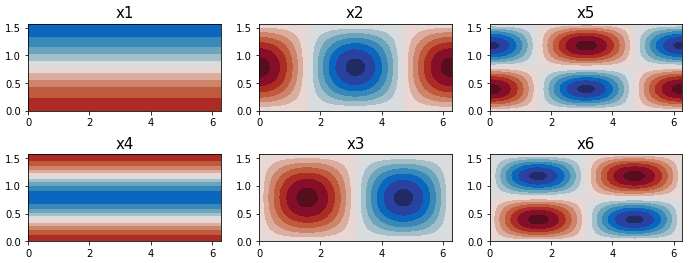
Figure A1 The real-valued basis functions used in the spectrally truncated CdV79 system, plotted as streamfunctions.

Although up to this point our approximations have been motivated well physically, we cannot rigorously justify introducing such a drastic truncation without resorting to self-interest: such a system is much easier to study and can be understood in more detail than a high-dimensional model. Nonetheless, we may reason that any phenomena observed in this truncated model, which will have to derive solely from the dynamics of the largest scales, may have analogues in the true atmospheric circulation, although there they will be shaped and influenced by coupling to smaller scales. The resulting basis functions are shown in Fig. A1.

Concretely, while the true spectral equation for the largest wave modes, Eq. (A22), contains an infinite number of non-linear coupling terms, after truncation we are reduced to only 36 such terms, representing only interactions between the resolved modes: the ability for small scales to feed vorticity into the untruncated large scales is neglected.

We choose our linear relaxation to be zonally symmetric, representing the forcing effect of the pole-to-equator temperature gradient. We choose our orography to include a single peak straddling the periodic boundary, with a trough in the centre of the domain. $h(x,y)=\mathit{\gamma }\sqrt{\mathrm{2}}\cos \left(x\right)\sin \left(\frac{y}{b}\right)$ (this is shown in Fig. A2).

Figure A2 The orographic profile used in the CdV79 system, with a trough in the centre of the domain and a ridge over the periodic boundary. Sub-panels show cross sections across the domain, following the dotted black lines.

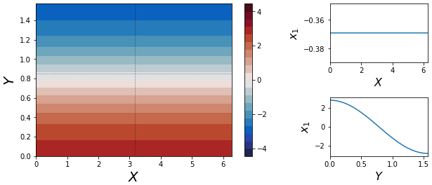
Figure A3 The background state in the Crommelin 1904 formulation of the CdV79 system. It is zonally symmetric and represents the impact of the meridional temperature gradient. Again, sub-panels show cross sections across the domain, following the dotted black lines.

Obtaining the coefficients in Eq. (A22) is now simply a matter of calculating integrals but is very involved and is best performed using symbolic computation software (an implementation using SymPy (Meurer et al., 2017) can be found at https://github.com/joshdorrington/Thesis_materials/blob/main/10d_mode_derivation.ipynb, last access: 3 February 2023). After computing coefficients, we now diverge slightly from CdV79, transforming our variables to a real basis, as in C04, given by

$$\begin{array}{ll}{x}_{\mathrm{1}}=\frac{\mathrm{1}}{b}{\mathrm{\Phi }}_{\mathrm{0},\mathrm{1}}& x_{\mathrm{4}}=\frac{\mathrm{1}}{b}{\mathrm{\Phi }}_{\mathrm{0},\mathrm{2}}\\ x_{\mathrm{2}}=\frac{\mathrm{1}}{\sqrt{\mathrm{2}}b}({\mathrm{\Phi }}_{\mathrm{1},\mathrm{1}}+{\mathrm{\Phi }}_{-\mathrm{1},\mathrm{1}})& x_{\mathrm{3}}=\frac{i}{\sqrt{\mathrm{2}}b}({\mathrm{\Phi }}_{\mathrm{1},\mathrm{1}}-{\mathrm{\Phi }}_{-\mathrm{1},\mathrm{1}})\\ x_{\mathrm{5}}=\frac{\mathrm{1}}{\sqrt{\mathrm{2}}b}({\mathrm{\Phi }}_{\mathrm{1},\mathrm{2}}+{\mathrm{\Phi }}_{-\mathrm{1},\mathrm{2}})& x_{\mathrm{6}}=\frac{i}{\sqrt{\mathrm{2}}b}({\mathrm{\Phi }}_{\mathrm{1},\mathrm{2}}-{\mathrm{\Phi }}_{-\mathrm{1},\mathrm{2}}).\end{array}$$

This transformation is purely cosmetic; the behaviour of the system is unchanged. At the end of this process we obtain an explicit six-equation system:

$$\begin{array}{}\text{(A23)}& \textcolor{red}{},\end{array}$$

where colours encode the linear relaxation (green), Coriolis forces (blue), orographic impacts (orange), and non-linear advection (red). We see that there are far fewer than the 36 promised non-linear terms per equation: most quadratic interactions integrated over the domain vanish due to symmetry considerations. $\mathit{\left\{}{\mathit{\alpha }}_n\mathit{\right\}},\mathit{\left\{}{\mathit{\beta }}_n\mathit{\right\}},\mathit{\left\{}{\mathit{\delta }}_n\mathit{\right\}},\mathit{\left\{}{\mathit{\gamma }}_n\mathit{\right\}},\mathit{\left\{}\stackrel{\mathrm{̃}}{{\mathit{\gamma }}_n}\mathit{\right\}}$, and ϵ are simple geometric constants of 𝒪(1) given in C04.

There are now a number of dimensionless free parameters in the model, which we set equal to the values used in K14 and C04:

• $x_i^{*}$ is the forcing vector, representing thermal relaxation towards a background state. We use a zonally symmetric forcing profile with x₁=0.95 and $x_{\mathrm{4}}=-\mathrm{0.76095}$; all other terms are zero (shown in Fig. A3).

• C is the thermal relaxation timescale, set to C=0.1, describing a damping time of ∼10 d.

• γ is the orographic amplitude, set to γ=0.2, corresponding to a 200 m amplitude.

• β is the Coriolis parameter, set to β=1.25, defining a central latitude of 45^∘.

• b defines the channel half-width, set to b=0.5, which gives a channel of 6300 km × 1600 km.

Appendix B: Impact of a Gaussian perturbation on exponential growth

In Sect. 3 we found that

$$\begin{array}{}\text{(B1)}& \langle \mathrm{\Delta }t\rangle =-\underset{-\mathrm{\infty }}{\overset{\mathrm{\infty }}{\int }}{\displaystyle \frac{\mathrm{1}}{\mathrm{2}}}\left|{\displaystyle \frac{d^{\mathrm{2}}G}{d(\mathrm{\Delta }x{)}^{\mathrm{2}}}}\right|\cdot P\left(\mathrm{\Delta }x\right)d\mathrm{\Delta }x=-I.\end{array}$$

If we consider x to be undergoing exponential growth and subject it to a Gaussian perturbation so that $x=f\left(t\right)=x_{\mathrm{0}}{e}^{\mathit{\lambda }t}$, and $P\left(\mathrm{\Delta }x\right)=\mathcal{N}(\mathrm{0},\mathit{\sigma })$, then we can obtain an analytical form for Δt. Remembering that $G_p\left(\mathrm{\Delta }x\right)=g(x_{\mathrm{p}}+\mathrm{\Delta }x)-g\left(x_{\mathrm{p}}\right)$, and seeing that $g\left(x\right)=\frac{\mathrm{1}}{\mathit{\lambda }}\log \left(\frac{x}{x_{\mathrm{0}}}\right)$, we have

$$\begin{array}{}\text{(B2)}& \langle \mathrm{\Delta }t\rangle =\underset{x_{\mathrm{0}}}{\overset{x_{\mathrm{c}}}{\int }}{\displaystyle \frac{\mathrm{1}}{\mathit{\lambda }}}\log \left({\displaystyle \frac{x}{x_{\mathrm{p}}}}\right)\cdot {\displaystyle \frac{\mathrm{1}}{\mathit{\sigma }\sqrt{\mathrm{2}\mathit{\pi }}}}{e}^{-\frac{\mathrm{1}}{\mathrm{2}}{\left(\frac{x-x_{\mathrm{p}}}{\mathit{\sigma }}\right)}^{\mathrm{2}}}\mathrm{d}x.\end{array}$$

We transform our variables to $w=\frac{\mathrm{\Delta }x}{\mathit{\sigma }}=\frac{x-x_{\mathrm{p}}}{\mathit{\sigma }}$, which implies $\frac{x}{x_{\mathrm{p}}}=\frac{x_{\mathrm{p}}+\mathit{\sigma }w}{x_{\mathrm{p}}}=\mathrm{1}+\frac{\mathit{\sigma }}{x_{\mathrm{p}}}w$ and $dx=\mathit{\sigma }\cdot \mathrm{d}w$. Our limits of integration become $w_{\mathrm{0}}=\frac{x_{\mathrm{0}}-x_{\mathrm{p}}}{\mathit{\sigma }}<\mathrm{0}$ and $w_{\mathrm{c}}=\frac{x_{\mathrm{c}}-x_{\mathrm{p}}}{\mathit{\sigma }}>\mathrm{0}$.

If, as in the main text, we assume σ is small relative to a typical length scale of x (that is the perturbation is vanishingly unlikely to force the system into the chaotic regime directly), then these limits will be very large in absolute magnitude. Given this and the exponentially decaying tails of the Gaussian distribution, we approximate $w_{\mathrm{0}}\approx -\mathrm{\infty }$, $w_{\mathrm{c}}\approx +\mathrm{\infty }$. This gives us

$$\begin{array}{}\text{(B3)}& \langle \mathrm{\Delta }t\rangle ={\displaystyle \frac{\mathrm{1}}{\mathit{\lambda }\sqrt{\mathrm{2}\mathit{\pi }}}}\underset{-\mathrm{\infty }}{\overset{+\mathrm{\infty }}{\int }}\log \left(\mathrm{1}+{\displaystyle \frac{\mathit{\sigma }}{x_{\mathrm{p}}}}w\right)\cdot e^{-\frac{w^{\mathrm{2}}}{\mathrm{2}}}\mathrm{d}w.\end{array}$$

While not directly integrable, we can make progress by Taylor-expanding the logarithm. Firstly we recognise that as the Gaussian distribution is even in w, then all odd terms in the Taylor expansion will vanish. Secondly we note that $\frac{\mathit{\sigma }}{x_{\mathrm{p}}}w=\frac{\mathrm{\Delta }x}{x_{\mathrm{p}}}$ will be small if, as above, σ is small, so we can drop terms of fourth order and higher in w. Thus we end up with

$$\begin{array}{}\text{(B4)}& \langle \mathrm{\Delta }t\rangle ={\displaystyle \frac{-{\mathit{\sigma }}^{\mathrm{2}}}{\mathrm{2}\mathit{\lambda }{x}_{\mathrm{p}}^{\mathrm{2}}\sqrt{\mathrm{2}\mathit{\pi }}}}\underset{-\mathrm{\infty }}{\overset{+\mathrm{\infty }}{\int }}{w}^{\mathrm{2}}\cdot e^{-\frac{w^{\mathrm{2}}}{\mathrm{2}}}\mathrm{d}w,\end{array}$$

which, from any book of identities, we can find gives

$$\begin{array}{}\text{(B5)}& \langle \mathrm{\Delta }t\rangle ={\displaystyle \frac{-{\mathit{\sigma }}^{\mathrm{2}}}{\mathrm{2}\mathit{\lambda }{x}_{\mathrm{p}}^{\mathrm{2}}\sqrt{\mathrm{2}\mathit{\pi }}}}\cdot \sqrt{\mathrm{2}\mathit{\pi }}={\displaystyle \frac{-{\mathit{\sigma }}^{\mathrm{2}}}{\mathrm{2}\mathit{\lambda }{x}_{\mathrm{p}}^{\mathrm{2}}}}.\end{array}$$