The joint application of a metaheuristic algorithm and a Bayesian statistics approach for uncertainty and stability assessment of nonlinear magnetotelluric data

In this paper, we have developed three algorithms, namely hybrid weighted particle swarm optimization (wPSO) with the gravitational search algorithm (GSA), known as wPSOGSA; GSA; and PSO in MATLAB to interpret one-dimensional magnetotelluric (MT) data for some corrupted and non-corrupted synthetic data, as well as two examples of MT field data over different geological terrains: (i) geothermally rich area, island of Milos, Greece, and (ii) southern Scotland due to the occurrence of a significantly high electrical conductivity anomaly under crust and upper mantle, extending from the Midland Valley across the Southern Uplands into northern England. Even though the fact that many models provide a good fit in a large predefined search space, specific models do not fit well. As a result, we used a Bayesian statistical technique to construct and assess the posterior probability density function (PDF) rather than picking the global model based on the lowest misfit error. The study proceeds using a 68.27 % confidence interval for selecting a region where the PDF is more prevalent to estimate the mean model which is more accurate and close to the true model. For illustration, correlation matrices show a significant relationship among layer parameters. The findings indicate that wPSOGSA is less sensitive to model parameters and produces more stable and reliable results with the least uncertainty in the model, compatible with existing borehole samples. Furthermore, the present methods resolve two additional geologically significant layers, one highly conductive (less than 1.0 Ωm) and another resistive (300.0 Ωm), over the island of Milos, Greece, characterized by alluvium and volcanic deposits, respectively, as corroborated by borehole stratigraphy.

1 Introduction

The magnetotelluric (MT) method is a natural source electromagnetic method that explores various natural resources, namely hydrocarbon, minerals, geothermal prospects, groundwater, and metalliferous ores, etc. (Nabighian and Asten, 2002; Simpson and Bahr, 2005). Due to its instability, non-unique solution, and algorithm sensitivity, MT data interpretation is thought-provoking. Many researchers have attempted and developed various inversion algorithms to interpret and improve the model accuracy, convergence speed, and stability and reduce the uncertainty of the solutions (Kirkpatrick et al., 1983; Constable et al., 1987; Rodi and Mackie, 2001; Li et al., 2018; Zhang et al., 2019; Khishe and Mosavi, 2020). There are mainly two categories of the inversion algorithm: first, the local optimization methods, namely the conjugate gradient, Levenberg–Marquardt/ridge regression, the Gauss-Newton algorithm, the steepest descent, and Occam's inversion, which require a good initial guess (Shaw and Srivastava, 2007; Wen et al., 2019; Roy and Kumar, 2021). Another category is global optimization techniques (i.e., ant colony optimization, genetic algorithm, particle swarm optimization, gravitational search algorithm, and simulated annealing, etc.), which do not require an initial guess. Many researchers have carried out numerous metaheuristic optimization algorithms to invert MT data (Dosso and Oldenburg, 1991; Pérez-Flores and Schultz, 2002; Miecznik et al., 2003; Sen and Stoffa, 2013). These algorithms are inspired by natural phenomena and have various geophysical applications, including particle swarm optimization (Kennedy and Eberhart, 1995; Essa et al., 2023), the genetic algorithm (Whitley, 1994), Bat algorithm (Yang, 2010a; Essa and Diab, 2023), differential evolution (Storn and Price, 1997), biogeographically based optimization (Simon, 2008), the firefly algorithm (Yang, 2010b), grey wolf optimizer (Mirjalili et al., 2014), ant colony optimization (Colorni et al., 1991), the gravitational search algorithm (Rashedi et al., 2009), and the novel barnacles mating optimizer algorithm (Ai et al., 2022).

However, unique characteristics, namely exploration and exploitation, persist in any global optimization algorithm. For example, the particle swarm optimization (PSO) algorithm has a very high potential for exploitation, which implies that the algorithm performs well in a local search but is inferior in exploration (S̨enel et al., 2019). This suggests that the algorithm has a limited capacity to estimate the best model in an extensive search range. Because of low exploration characteristics, it gets trapped at the local minima (Mirjalili and Hashim, 2010). So, integrating the two algorithms with opposite characteristics is the best way to balance exploration and exploitation characteristics to achieve better solutions than the results obtained from an individual algorithm.

Here, we utilized weighted hybrid PSOGSA (wPSOGSA), a new global optimization method that takes into account the algorithm based on natural behavior seen in birds, fish, and insects, known as PSO, and gravity-based Newton's law (with high exploration capability), known as the gravity search algorithm (GSA). Researchers interested in artificial intelligence and developing effective optimization algorithms for comparative analysis of different metaheuristic algorithms (Pace et al., 2022) have been drawn to notable characteristics in such social behavior. The wPSOGSA, PSO, and GSA are used to estimate the resistivity distribution of 1D multi-layered Earth models using synthetic (noise-free and noisy) data for three- and four-layer cases, taken from Shaw and Srivastava (2007) and Xiong et al. (2018), respectively, and field MT sounding data for six- and four-layer cases, taken from Hutton et al. (1989) and Jones and Hutton (1979), respectively.

Furthermore, numerous (here 10 000) models that fit well are optimized to obtain the mean model, which is preceded by calculating the posterior probability density function (PDF) based on Bayesian concepts using all accepted models to find the optimal mean solution with the least uncertainty, as well as a correlation matrix to determine the relationships among the layer parameters. Thus, the research reveals that the wPSOGSA method may be utilized to provide a more accurate and reliable model with superior stability, a quick rate of convergence, and the least amount of model uncertainty.

2 Data and methodology

2.1 Synthetic and field data

Different MT datasets are utilized to evaluate the proposed wPSOGSA's effectiveness, sensitivity, stability, and robustness in outlining the genuine subsurface structure. These datasets are noise-free and Gaussian noise synthetic data produced for several geological formations, and two MT field data have been optimized for analysis.

To demonstrate and evaluate the robustness of the present algorithms, we have generated a synthetic MT apparent resistivity and apparent phase dataset without noise and with noise levels (10 % and 20 % noise) considering a three-layer typical continental crustal model with a total thickness of 33 000 m (i.e., 33.0 km) and a resistivity of the upper crust of 30 000.0 Ωm with 15 000 m (i.e., 15 km) thickness (high resistive layer) and a resistivity of the middle crust of 5000.0 Ωm with 18 000 m (i.e., 18.0 km) thickness (reasonable low resistive layer) underlain by 1000 Ωm (low resistive) half space taken from Shaw and Srivastava (2007).

For the second example of the synthetic data, a typical four-layer HK-type of Earth model taken from Xiong et al. (2018) is generated by forward modeling equations for the demonstration of the wPSOGSA, PSO, and GSA, and their performance is compared with improved differential evolution (IDE) results obtained by Xiong et al. (2018).

We utilized the first example of field data taken from Hutton et al. (1989) on the island of Milos, Greece. Milos is a part of the South Aegean active volcanic arc, an example of an emergent volcanic edifice (Stewart and McPhie, 2006) formed by monogenetic effusive and explosive magmatism pulses. Milos is the world's biggest exporter of bentonite, and it also has a diverse variety of metalliferous and non-metalliferous mineral reserves. It is a conserved on-land laboratory for studying shallow underwater hydrothermal ore-forming processes. The accompanying shallow subsurface hydrothermal venting fields have had significantly less attention. Dawes (1986) used magnetotelluric data to assess the resistivity structure of the geothermal area on Milos' west side. With around 3.0 km spacing, 37 MT probes in the bandwidth of 100–0.01 Hz and 12 investigations in the bandwidth of 0.01–0.0001 Hz were installed, along with various profiles that were perpendicular to the Zephyria graben in the W–E direction, as well as along the graben in the S–N direction (Hutton et al., 1989).

Another field example of MT data from Jones and Hutton (1979) was picked to illustrate our technique from Newcastleton (55.196^∘ N, 2.796^∘ W, in geographic coordinates), Southern Uplands of Scotland. By the Southern Uplands fault, the Southern Uplands are isolated from the Midland Valley. The bulk of the Southern Uplands comprises Silurian–lower Paleozoic sedimentary deposits such as greywackes and shales that originated in the Iapetus Ocean during the late Neoproterozoic and early Paleozoic geologic eras. These rocks emerged from the seafloor as an accretionary wedge during the Caledonian orogeny. The majority of the rocks are coarse greywacke, a kind of sandstone that has been poorly metamorphosed and contains angular quartz, feldspar, and small rock fragments. The Midland Valley and northern England, on the other hand, are known for their thick Carboniferous layers, which are used to measure coal.

2.2 Forward modeling – magnetotelluric formulation for 1-D Earth

The ability to formulate an effective inversion method requires a thorough understanding of the forward modeling technique for the issue of interest. Factors like frequency range, actual resistivity, and layer thickness are used to create datasets of synthetic MT apparent resistivity, ρ_a(ω), and apparent phase, φ_a(ω). The electromagnetic impedance (Z) for layered structures is described in terms of an orthogonal electric field, magnetic field, wavenumber (k), reflection coefficient (R), and exponent factor (τ_f) with angular frequency (ω) as (Ward and Hohmann, 1988)

$$\begin{array}{}\text{(1)}& Z={\displaystyle \frac{{\mathit{\mu }}_{\mathrm{0}}\mathit{\omega }}{k}}={\displaystyle \frac{E_x}{H_y}}=-{\displaystyle \frac{E_y}{H_x}},\end{array}$$

where the wavenumber $\left(k\right)=\sqrt{-i{\mathit{\mu }}_{\mathrm{0}}\mathit{\omega }/\mathit{\rho }}$, E_x and E_y are components of the electric field, and H_x and H_y are the components of the magnetic field.

If displacement currents are not taken into account, Eq. (1) becomes

$$\begin{array}{}\text{(2)}& \begin{array}{rl}Z& ={\displaystyle \frac{{\mathit{\mu }}_{\mathrm{0}}\mathit{\omega }}{\sqrt{-i{\mathit{\mu }}_{\mathrm{0}}\mathit{\omega }/\mathit{\rho }}}}=\sqrt{i{\mathit{\mu }}_{\mathrm{0}}\mathit{\omega }\mathit{\rho }}\\ & =\sqrt{{\mathit{\mu }}_{\mathrm{0}}\mathit{\omega }\mathit{\rho }}{e}^{\frac{i\mathit{\pi }}{\mathrm{4}}}=\mathit{\omega }{\displaystyle \frac{\left(\mathrm{1}-R{\mathit{\tau }}_{\mathrm{f}}\right)}{\left(\mathrm{1}+R{\mathit{\tau }}_{\mathrm{f}}\right)}}.\end{array}\end{array}$$

Noisy impedance is calculated by the following equation:

$$\begin{array}{}\text{(3)}& Z_{\mathrm{noisy}}=Z+Z\times \left(\mathrm{2}\times \text{rand}-\mathrm{1}\right)\times {\mathrm{noise}}_{\mathrm{percent}}.\end{array}$$

If the angle between impedance phase with E_x is 45^∘, then the resistivity (ρ) in half space of impedance Z(ω) and time period (T) can be written as

$$\begin{array}{}\text{(4)}& \mathit{\rho }\left(\mathit{\omega }\right)={\displaystyle \frac{\mathrm{1}}{{\mathit{\mu }}_{\mathrm{0}}\mathit{\omega }}}{\left|Z\left(\mathit{\omega }\right)\right|}^{\mathrm{2}}={\displaystyle \frac{\mathrm{0.2}T}{{\mathit{\mu }}_{\mathrm{0}}}}{\left|{\displaystyle \frac{E_x}{H_y}}\right|}^{\mathrm{2}}.\end{array}$$

Thus, the apparent resistivity and apparent phase are defined (Cagniard, 1953; Ward and Hohmann, 1988) as follows:

$$\begin{array}{}\text{(5)}& {\displaystyle }\begin{array}{rl}& \text{apparent resistivity, }\\ & {\mathit{\rho }}_{\mathrm{a}}\left(\mathit{\omega }\right)={\displaystyle \frac{\mathrm{1}}{{\mathit{\mu }}_{\mathrm{0}}\mathit{\omega }}}\left[Z\left(\mathit{\omega }\right)Z^{\ast }\left(\mathit{\omega }\right)\right],\end{array}\text{(6)}& {\displaystyle }\begin{array}{rl}& \text{and apparent phase,}\\ & {\mathit{\phi }}_{\mathrm{a}}\left(\mathit{\omega }\right)={\tan }^{-\mathrm{1}}\left({\displaystyle \frac{\text{img}\left(Z\left(\mathit{\omega }\right)\right)}{\text{real}\left(Z\left(\mathit{\omega }\right)\right)}}\right),\end{array}\end{array}$$

where the exponent factor ${\mathit{\tau }}_{\mathrm{f}}=\exp \left(-\mathrm{2}\mathit{\gamma }h\right)$, the induction parameter $\mathit{\gamma }=\sqrt{i\mathit{\omega }{\mathit{\mu }}_{\mathrm{0}}/\mathit{\rho }}$, h is the layer thickness, μ₀ is the magnetic permeability for free space, Z^∗ is the complex conjugate of impedance, and “rand” is used for generating a random number between 0 and +1.

2.3 Global optimization technique

The techniques that we have used for the joint modeling of metaheuristic global optimization, namely PSO, GSA, and wPSOGSA in Step 1 and posterior Bayesian probability density function technique in Step 2, obtain the global model by utilizing the synthetic data generated by using forward modeling and field MT apparent resistivity and phase curves, depicted in the schematic diagram (Fig. 1).

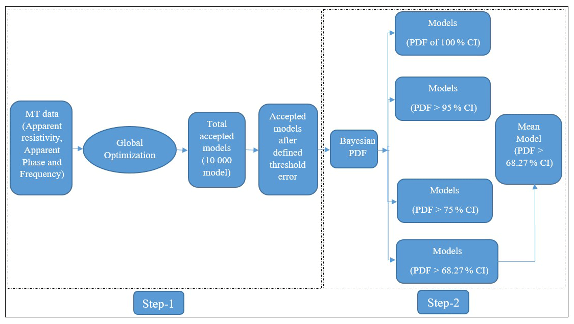
Figure 1 Schematic diagram demonstrating the essential processes considered for the joint modeling of metaheuristic global optimization (Step 1) and the posterior PDF technique (Step 2) to obtain the global model by utilizing synthetic and field MT data.

2.4 Optimization and error estimation

In the present study, we have implemented a new innovative global optimization technique known as wPSOGSA, in which swarm particles and mass particles provide the best particle, i.e., the best model. The best model is chosen based on the fitness of the particles, and the cost function or objective function is used to estimate this fitness. Thus the magnetotelluric (MT) inverse problem can be formulated through the forward modeling operator, f(x), to achieve the resistivity model, which illuminates the observed data ρ and φ. This operator combines the problem of physics and inverts the observed apparent resistivity and phase data to the resistivity–depth model, x, as

$$\begin{array}{}\text{(7)}& \left(\mathit{\rho },\mathit{\phi }\right)=f\left(\mathbf{x}\right).\end{array}$$

The cost function (fitness of the particle) is a mathematical relation between observed and calculated data, and the root mean square error (RMSE) is defined as follows:

$$\begin{array}{}\text{(8)}& \text{RMSE}=\sqrt{\left\{{\displaystyle \frac{(\mathit{\rho }-{\mathit{\rho }}_{\mathrm{C}}{)}^{\mathrm{2}}}{N}}+{\displaystyle \frac{(\mathit{\phi }-{\mathit{\phi }}_{\mathrm{C}}{)}^{\mathrm{2}}}{N}}\right\}},\end{array}$$

where N is the total observed data points, ρ and φ are the observed apparent resistivity and phase, and ρ_C and φ_C are the computed apparent resistivity and phase data.

2.5 Particle swarm optimization

The particle swarm optimization (PSO) technique is a widespread evolutionary optimization approach for determining the optimal global solution to a nonlinear inverse problem (Kennedy and Eberhart, 1995). This technique is analogous to the particle's natural behavior in search of food with the help of collaborative support from the population represented by geophysical resistivity solutions/models (known as particles) in a swarming group. The best model/position obtained among the particles so far is stored for each iteration, which helps in search of the global best solution, defined by the fitness of each particle estimated using Eq. (8). The velocity and location of the kth particle at the tth iteration are defined as

$$\begin{array}{}\text{(9)}& {\displaystyle }\begin{array}{rl}{v}_k\left(t+\mathrm{1}\right)& =w{v}_k\left(t\right)+c_{\mathrm{1}}\times \text{rand}\times \left(x_{\mathrm{p}}-x_k\left(t\right)\right)\\ & +c_{\mathrm{2}}\times \text{rand}\times \left(x_{\mathrm{g}}-x_k\left(t\right)\right)\end{array}\text{(10)}& {\displaystyle }{x}_k\left(t+\mathrm{1}\right)=x_k\left(t\right)+v_k\left(t+\mathrm{1}\right),\end{array}$$

where w is the inertia weight set between 0 and 1; c₁ and c₂ are a personal learning coefficient and a global learning coefficient, respectively; v_k(t) is the velocity of the kth particle at tth iteration; rand is used for a random number between 0 and 1; x_p is the present best solution, x_g is the global best solution, and x_k(t) is the position of the kth particle at the tth iteration. Particles change their position at each iteration to approach an optimum solution. The first, second, and third terms in Eq. (9) represent exploratory ability, private thought, and particle collaboration, respectively.

2.6 Gravitational search algorithm

The gravitational search algorithm (GSA) is a metaheuristic algorithm based on Newton's gravitational law (Rashedi et al., 2009), which states that mass particles attract each other with a gravitational force that is directly proportional to the product of their masses and inversely proportional to the square of the distance between them. It signifies that massive particles (here, particle represents the resistivity layer model/solution) attract the neighboring lighter particles. Similar to PSO, the gravitational search optimizer works with a population of particles known as mass particles in the universe. Thus the best model, solution, or particle is achieved among the mass particles. The best model is defined by each particle's capability (i.e., the fitness), calculated using Eq. (8). The initialization of their position in the search spaces is given by

$$\begin{array}{}\text{(11)}& x=\text{rand}\left(N,D\right)\times \left(\text{up}-\text{down}\right)+\text{down},\end{array}$$

where N and D are the number of particles and models, i.e., the dimension of the model, and “up”, and “down” are the upper and lower limit of the search range, respectively.

During execution time, the gravitational acting force on agent kth from agent jth at a specific time (t) is defined as

$$\begin{array}{}\text{(12)}& F_{k,j}\left(t\right)=G\left(t\right){\displaystyle \frac{M_{\mathrm{p},k}\left(t\right)\cdot M_{\mathrm{a},j}\left(t\right)}{R_{k,j}\left(t\right)+\mathit{ϵ}}}\left(x_j\left(t\right)-x_k\left(t\right)\right),\end{array}$$

where M_a,j and M_p,k are the active and passive gravitational masses for particle j and k, respectively; x_j(t) is the position of the particle j at a time t for various parameters; R_k,j (t) is the Euclidian distance between two particles; and ε is a small constant.

Here, the gravitational constant G(t) at a specific time t is defined as in Kunche et al. (2015), and the acceleration of the kth agent at the tth iteration for models is ac_k(t), defined as

$$\begin{array}{}\text{(13)}& {\text{ac}}_k\left(t\right)={\displaystyle \frac{F_k\left(t\right)}{M_k\left(t\right)}},\end{array}$$

where F_k,j(t) the gravitational acting force on agent k from agent j, and M_k(t) is the mass of the object at a specific time (t).

$$\begin{array}{}\text{(14)}& G\left(t\right)=G_{\mathrm{0}}\times \exp \left(-\mathit{\alpha }\times {\displaystyle \frac{\text{iter}}{\text{maxiter}}}\right),\end{array}$$

where α, G₀, “iter”, and “maxiter” are descending coefficients, starting value of gravitational constant, current iteration, and maximum iterations, respectively.

The following equations are used to update the particle's velocity and location:

$$\begin{array}{}\text{(15)}& {\displaystyle }{v}_k\left(t+\mathrm{1}\right)=\text{rand}\times v_k\left(t\right)+{\text{ac}}_k\left(t\right)\text{(16)}& {\displaystyle }{x}_k\left(t+\mathrm{1}\right)=x_k\left(t\right)+v_k\left(t+\mathrm{1}\right).\end{array}$$

All the particles are randomly placed in the search range using Eq. (11), and then the particle's velocity is initialized. Meanwhile, the gravitational constant, total forces, and acceleration are computed, and the locations are updated. The end criterion, the misfit error (i.e. 10⁻⁹), is taken in our study.

2.7 Weighted hybrid PSOGSA (wPSOGSA)

The weighted hybrid of PSO and GSA, known as wPSOGSA, integrates two essential characteristics, exploration (i.e., the ability of an algorithm to search the whole range of a given parameter) and exploitation (i.e., the ability to converge the solution nearest to the best solution) of the global optimization algorithm that increases its efficiency and converges the objective function to achieve global minima. The velocity and location of the particles updated in the wPSOGSA are illustrated in the schematic diagram (see Fig. 2).

The wPSOGSA combines the characteristic of social thinking of PSO and the searching capability of GSA; thus, the particle's velocity is defined as

$$\begin{array}{}\text{(17)}& \begin{array}{rl}{v}_k\left(t+\mathrm{1}\right)& =w\times v_k\left(t\right)+c_{\mathrm{1}}\times \text{rand}\times {\text{ac}}_k\left(t\right)\\ & +c_{\mathrm{2}}\times \text{rand}\times (x_{\mathrm{g}}-x_k\left(t\right)),\end{array}\end{array}$$

where v_k(t) is the velocity of the particle k at iteration t, w is the weight function (i.e., the constant which helps to control the momentum of the algorithm to perform optimization properly), ac_k(t) is the acceleration of agent k, x_g is the best solution, and rand is a random number that lies between 0 and 1. At each iteration, particles updated their location to achieve the best solution defined as

$$\begin{array}{}\text{(18)}& x_k\left(t+\mathrm{1}\right)=x_k\left(t\right)+v_k\left(t+\mathrm{1}\right).\end{array}$$

The algorithm starts by randomly initializing the velocity, mass, and acceleration of the particles. The cost function is evaluated for all particles for specified iterations to get the most optimal solution, and inverted results are updated at each iteration. Equations (12), (17), and (18) are used to update the gravitational force, velocity, and location of particles after initialization. However, the velocity and position stop updating their values when the algorithm converge, and the least error of the cost function is reached.

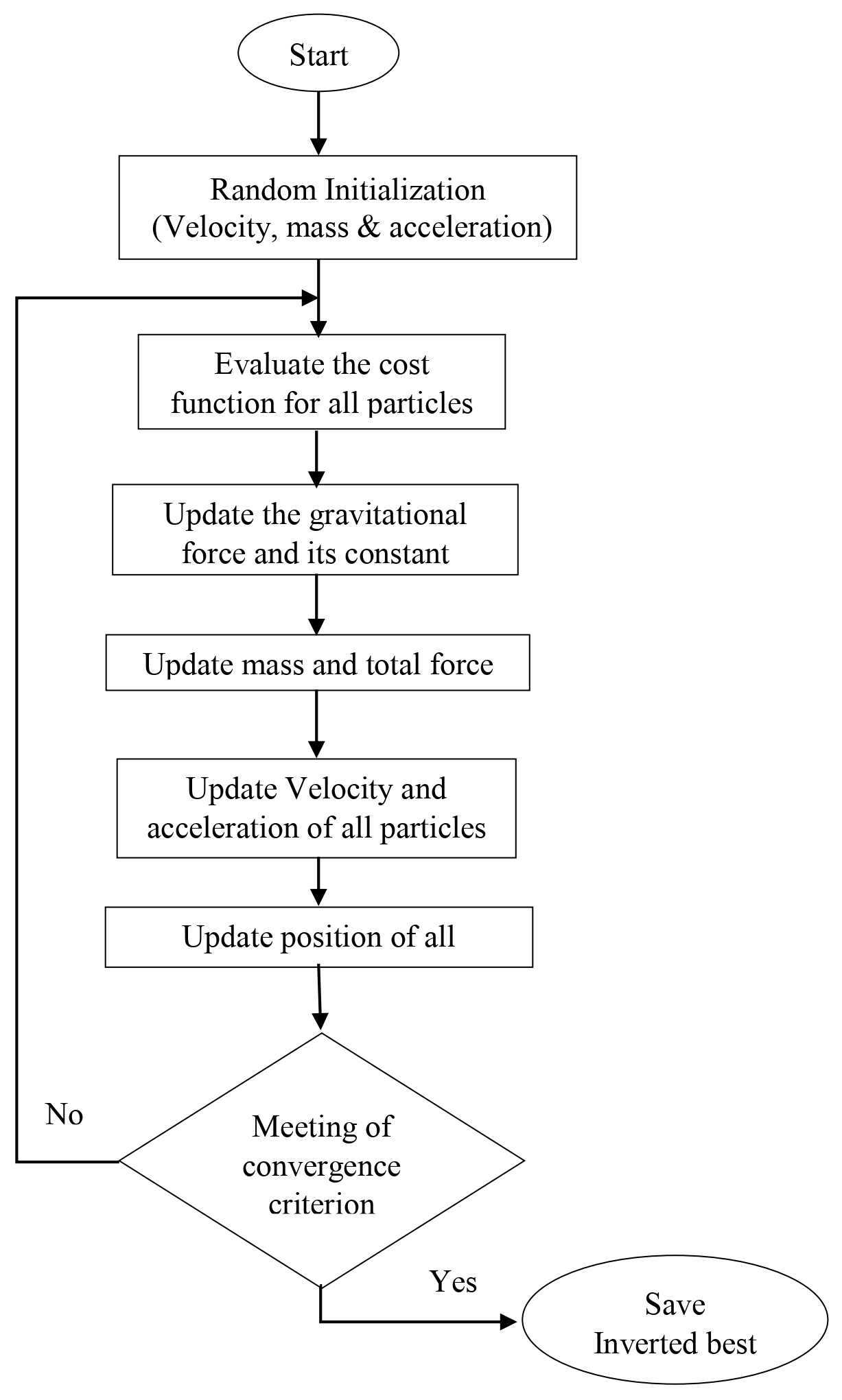
Figure 2 Flow chart of the weighted hybrid particle swarm optimization and gravity search algorithm, known as wPSOGSA (after Mirjalili and Hashim, 2010).

2.8 Bayesian probability density function

In a Bayesian framework, the probability distribution of the model parameters (known as posterior probability distribution) is computed using given observed data and models obtained from inversion. The posterior for a model is calculated using Bayes' theorem and previous model space information. Individual model parameter ranges are incorporated into the prior knowledge. The two fundamental stages in the Bayesian statistics method are the representation of previous knowledge as a probability density function and calculation of the likelihood functional derived from data misfit (Tarantola and Valette, 1982). Specific characteristics, such as the best fitting model, mean model, and correlation matrix, may be determined from posterior distribution of models. According to Bayes' theorem,

$$\begin{array}{}\text{(19)}& \text{posterior}=\text{prior}\times \text{likelihood}.\end{array}$$

As a result, our priori distribution function (f(μ)) for the parameter, x_u; mean priori information, M; and t², the mean uncertainty, is defined as

$$\begin{array}{}\text{(20)}& f\left(\mathit{\mu }\right)={\displaystyle \frac{\mathrm{1}}{\sqrt{\mathrm{2}\mathit{\pi }{t}^{\mathrm{2}}}}}\exp \left\{-{\displaystyle \frac{{\left(x_u-M\right)}^{\mathrm{2}}}{\mathrm{2}{t}^{\mathrm{2}}}}\right\},\end{array}$$

and the likelihood function is

$$\begin{array}{}\text{(21)}& f\left(X\mathrm{|}\mathit{\mu }\right)=\prod _{u=\mathrm{1}}^n{\displaystyle \frac{\mathrm{1}}{\sqrt{\mathrm{2}\mathit{\pi }{\mathit{\sigma }}^{\mathrm{2}}}}}\exp \left\{-{\displaystyle \frac{{\left(x_u-\mathit{\mu }\right)}^{\mathrm{2}}}{\mathrm{2}{\mathit{\sigma }}^{\mathrm{2}}}}\right\}.\end{array}$$

Hence the posterior density function calculated for a parameter (x_u) using mean (μ) and variance (σ²) defined (Lynch, 2007) as

$$\begin{array}{}\text{(22)}& f\left(\mathit{\mu }\mathrm{|}X\right)={\displaystyle \frac{\mathrm{1}}{\sqrt{t^{\mathrm{2}}{\mathit{\sigma }}^{\mathrm{2}}}}}\exp \left\{{\displaystyle \frac{-{\left(\mathit{\mu }-M\right)}^{\mathrm{2}}}{\mathrm{2}{t}^{\mathrm{2}}}}+{\displaystyle \frac{\sum _{u=\mathrm{1}}^n{\left(x_u-\mathit{\mu }\right)}^{\mathrm{2}}}{\mathrm{2}{\mathit{\sigma }}^{\mathrm{2}}}}\right\}.\end{array}$$

The posterior Bayesian PDF is calculated from accepted models within a set of parameters, as shown below:

$$\begin{array}{}\text{(23)}& P\left(X\mathrm{|}E\right)={\displaystyle \frac{P\left(X\right)L\left(E\mathrm{|}X\right)}{\sum _{X}P\left(X\right)L\left(E\mathrm{|}X\right)}},\end{array}$$

where P(X|E) is the posterior probability distribution of the parameter (X) given the evidence (E), P(X) is the prior information of (X), and L(E|X) is the likelihood function of X.

After the application of the PDF, the study further proceeds by choosing a confidence interval (CI) of 68.27 % that is based on the empirical rule, known as the 68–95–99.7 rule (Ross, 2009). The model parameters below 68.27 % CI are discarded, and the remaining parameters are used for determining the mean model and uncertainty. Thus, the mean model (P_j) is calculated using the best models having a PDF within a 68.27 % CI, defined in the following equation:

$$\begin{array}{}\text{(24)}& P_j=\exp {\displaystyle \frac{\mathrm{1}}{Nd}}\sum \ln \left(P_{j,k}\right).\end{array}$$

Here accepted models are used to calculate the correlation matrix (i.e., correlation among model parameters lie between −1 and 1) using the following equation (Tarantola, 2005):

$$\begin{array}{}\text{(25)}& \text{Cov}P\left(l,j\right)={\displaystyle \frac{\mathrm{1}}{Nd}}\sum \left(P_{l,k}-P_l\right)\left(P_{j,k}-P_l\right)\end{array}$$

and

$$\begin{array}{}\text{(26)}& \text{Cor}P\left(l,j\right)={\displaystyle \frac{\text{Cov}P\left(l,j\right)}{\sqrt{\text{Cov}P\left(l,l\right)\times \text{Cov}P\left(j,j\right)}}}.\end{array}$$

Here, N is the total number of models; d is used for the number of the layer parameters; and P_j,k is the jth model parameter of the kth model, where l and j both vary from 1 to d (number of layer parameters). CovP(l,j) is the covariance matrix between model parameters l and j, P_l,k is the lth model parameter of the kth model, and CorP(l,j) is the correlation matrix between model parameters l and j.

3 Results and analysis

The effectiveness, sensitivity, stability, and robustness of the proposed wPSOGSA in identifying the authentic subsurface structure are evaluated using various MT datasets. These datasets consist of synthetic data with no noise and Gaussian noise, which simulate different geological formations. Additionally, two MT field datasets have been optimized for analysis.

3.1 Application to synthetic MT data – three-layer case

The first example of synthetic MT data was executed for 10 000 runs, keeping the same lower and upper bounds as given in Table 1 and iterations to 1000. Figure 3 shows (a) the observed apparent resistivity with the computed data; (b) the observed apparent phase with the computed data; (c) the 1D inverted model by wPSOGSA (red color), GSA (green color), and PSO (blue color) with a true model (black color); and (d) the relation between the misfit and iterations for the noise-free synthetic data.

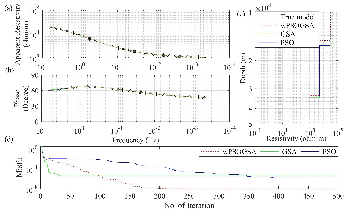
Figure 3 The inverted MT response by PSO (blue color), GSA (green color), and hybrid wPSOGSA (red color) with a true model (black color) over three-layer synthetic data as shown in (a) the observed and calculated apparent resistivity curve, (b) the observed and calculated apparent phase curve, (c) the 1D depth inverted model, and (d) the misfit error versus iterations.

The misfit curve as shown in Fig. 3d is gradually decreasing with increasing iterations and becomes constant where the algorithm converges. The PSO, GSA, and wPSOGSA converge at iterations 492, 35, and 316, with associated errors of $\mathrm{1.51}\times {\mathrm{10}}^{-\mathrm{6}}$, $\mathrm{3.97}\times {\mathrm{10}}^{-\mathrm{6}}$, and $\mathrm{1.035}\times {\mathrm{10}}^{-\mathrm{8}}$ and associated computational times of 27.06, 1.75, and 3.35 s, respectively. Thus, the curves show that wPSOGSA converges at the least RMSE. In contrast, PSO, GSA, and wPSOGSA using 10 % noisy synthetic data converge at 102, 88, and 358 iterations, with associated errors of 0.00435, 0.00439, and 0.00426 and associated computational times of 5.61, 4.40, and 3.80 s, respectively.

The 20 % noisy synthetic MT data were executed for 10 000 runs, keeping the same lower bound, upper bound, and iterations. The well-fitted inverted MT response (see Fig. 4) was as follows: (a) the corrupted synthetic and calculated apparent resistivity data, (b) the corrupted synthetic and calculated apparent phase data, (c) the inverted 1D depth model, and (d) convergence response in terms of misfit error versus iterations. We analyzed Fig. 4d and found that the PSO, GSA, and wPSOGSA using noisy synthetic data converge at iterations 236, 7, and 73, with associated errors of 0.0394, 0.0408, and 0.0393, respectively.

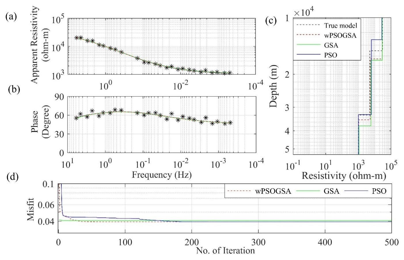
Figure 4 The inverted MT response by PSO (blue color), GSA (green color), and hybrid wPSOGSA (red color) with a true model (black color) over three-layer synthetic data with 20 % random noise as shown in (a) the observed and calculated apparent resistivity curve, (b) the observed and calculated apparent phase curve, (c) the 1D depth inverted model, and (d) the misfit error versus iterations.

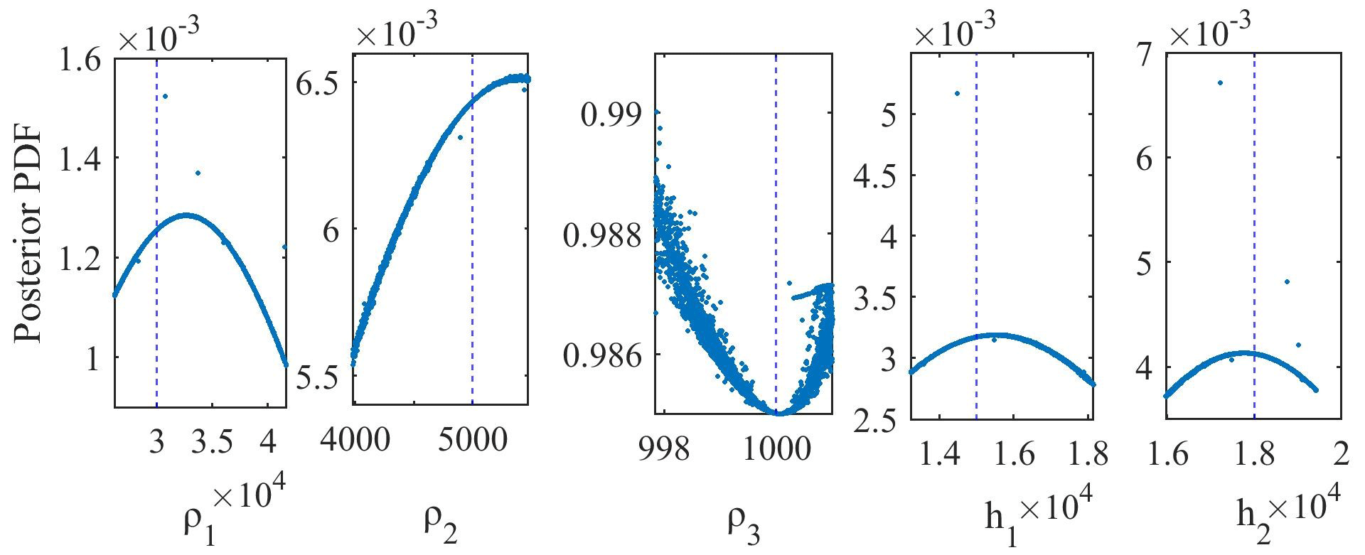
Figure 5 The posterior Bayesian probability density function (PDF) with 68.27 % CI for wPSOGSA for three-layered synthetic data.

3.1.1 Bayesian analysis and uncertainty in model parameters

Two methods are used to estimate a mean solution and uncertainty: one method is the mean solution for all accepted best-fitted solutions acquired from 10 000 runs for all three global optimization techniques; another method is the model derived from all approved solutions using the posterior Bayesian PDF within 1 standard deviation. To get the global best solutions in our study, we incorporated the posterior PDF based on the Bayesian approach to enhance the efficacy of the inverted model and minimize the uncertainty in the model. The process for obtaining the mean solution proceeds by selecting an initial threshold error, which is essential because the smaller the threshold value, the more significant the number of models with less uncertainty in the model parameters (Sharma, 2012). Thus, a more considerable threshold gives a lower number of models with enormous uncertainty in the model parameter (Sen and Stoffa, 1996; Sharma, 2012). The study proceeds by calculating the PDF for each parameter value using Eq. (22). In order to select values of each parameter that having a higher posterior PDF, a 68.27 % CI is used. The mean model obtained from selected model parameters is near to the actual model.

Figure 5 shows the output of the posterior Bayesian PDF, which selects model parameters with less error. The straight lines (dashed lines) present the actual value of the respective layer parameters. The first-layer thickness, second-layer thickness, and first-layer resistivity have higher uncertainties, i.e., 61.25 m, 51.47 m, and 210.61 Ωm, respectively, whereas the second-layer resistivity and third-layer resistivity have lower uncertainty, i.e., 17.71 and 0.03 Ωm, respectively.

Table 1 True model, search range, and inverted layer parameters by wPSOGSA, GSA, and PSO using different amounts of noisy (0 %, 10 %, and 20 %) synthetic MT apparent resistivity and apparent phase datasets for a three-layer Earth model.

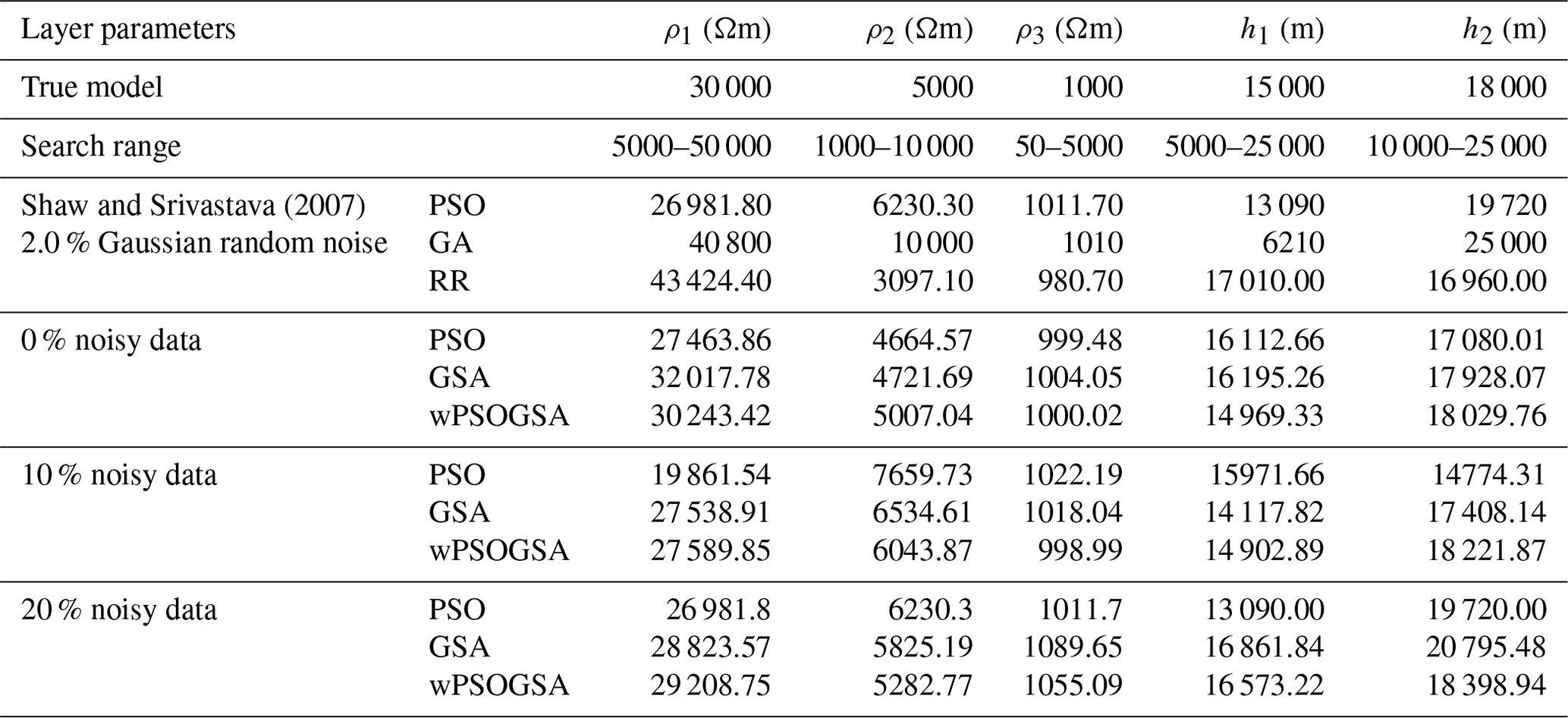
Table 1 shows the inverted layer parameters using wPSOGSA, GSA, and PSO for noise-free and noisy synthetic MT data based on the posterior Bayesian PDF, as well as the actual model and the search range. In addition, layered properties of synthetic data corrupted with 10 % and 20 % random noise are compared and statistically analyzed. Our findings, as shown in Table 1, were compared to those obtained using the genetic algorithm (GA), ridge regression (RR), and PSO by Shaw and Srivastava (2007), which consistently outperform GA and RR, which is closer to the genuine model.

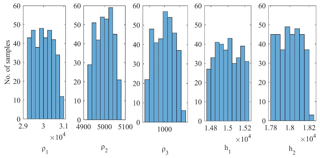
Figure 6 Histogram of selected models for misfit error below a defined threshold error of wPSOGSA.

The mean values of the accepted model parameters are 30 243.42±471.26, 5007.04±39.59, 1000.02±0.064, 14 969.33±136.82, and 18 029.76±114.90, and their associated amounts of uncertainty are 1.5 %, 0.78 %, 0.0064 %, 0.91 %, and 0.63 %. On the basis of a low posterior PDF and high uncertainty, we have taken (ρ₁) and (h₁) for the exercise to show the models are not biased to the selected models.

As well as being based on the histograms (see Fig. 6), the posterior PDF and uncertainty of the inverted layer parameters resistivity (ρ₁) and thickness (h₁) for the three-layered synthetic MT data have been taken to depict the global solution using presented algorithm. Here we prepared the cross-plots of ρ₁ versus h₁ using (a) wPSOGSA, (b) PSO, and (c) GSA, showing all accepted models (red circle), selected models with a misfit error of less than a threshold error of 10⁻⁴ (magenta circle), models of a PDF greater than 95 % (blue circle), models of a PDF greater than 75 % (green circle), models of a PDF greater than 68.27 % (yellow circle), and mean models, i.e., model parameters which have a PDF greater than 68.27 % (black asterisk), as shown in Fig. 7. It is noticed that all inverted results give the global solution, which has a good agreement with the true model, whereas wPSOGSA gives more accurate results than the other two algorithms, PSO and GSA, as shown in Table 2.

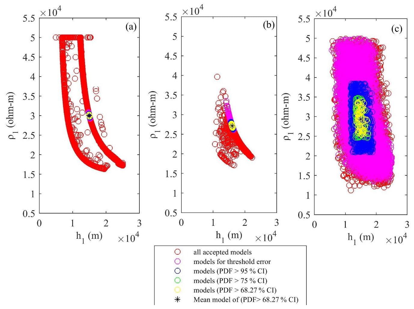
Figure 7 Cross-plots of thickness and resistivity of first layer for the three-layered synthetic resistivity model using (a) wPSOGSA, (b) PSO, and (c) GSA, displaying all accepted models (red circle), selected models with misfit error less than a threshold error (magenta circle), models with a PDF >95 % CI (blue circle), models with a PDF >75 % CI (green circle), models with a PDF >68.27 % CI (yellow circle), and the mean model, i.e., model parameters which have a PDF >68.27 % (black asterisk).

3.1.2 Sensitivity, correlation matrix, and model parameters

The accepted models, which have a posterior PDF value within 68.27 % CI, are used to calculate the correlation matrix. This correlation matrix gives the relationship among model parameters. Thus, the lower correlation value gives weak relation among the parameters and vice versa. The correlation matrix of PSO, GSA, and wPSOGSA was examined on one set of synthetic data, as shown in Figs. 8, 9, and 10, demonstrating the sensitivity among inverted model parameters. The value of correlation matrix, 1.0, indicates that the two parameters are strongly correlated.

Figure 8 shows that first-layer resistivity is correlated highly positively with a first-layer thickness (0.97) and second-layer thickness (0.98), while the second-layer resistivity (−0.99) and third-layer resistivity (−0.81) are substantially negative connected. Second-layer resistivity is correlated with the third-layer resistivity (0.87), which has a significant positive relationship, while second-layer resistivity has a significant negative correlation with the first-layer thickness (−0.99) and the second-layer thickness (−1.00). First-layer thickness (−0.92) and second-layer thickness (−0.90) are very negatively associated with third-layer resistivity, while first-layer thickness is extremely positively correlated with second-layer thickness (0.99).

Figure 9 indicates that first-layer resistivity is highly associated with second-layer thickness (1.00) and weakly with second-layer resistivity (−1.00), third-layer resistivity (−1.00), and first-layer thickness (−1.00). Second-layer resistivity (−1) is highly linked with a second-layer thickness (−1.00), while third-layer resistivity (1.00) and first-layer thickness are strongly correlated (1.00). Third-layer resistivity has a highly positive correlation with first-layer thickness (1.00) and a strong negative correlation with second-layer thickness (−1.00), whereas first-layer thickness has a significant negative correlation with second-layer thickness (−1.00).

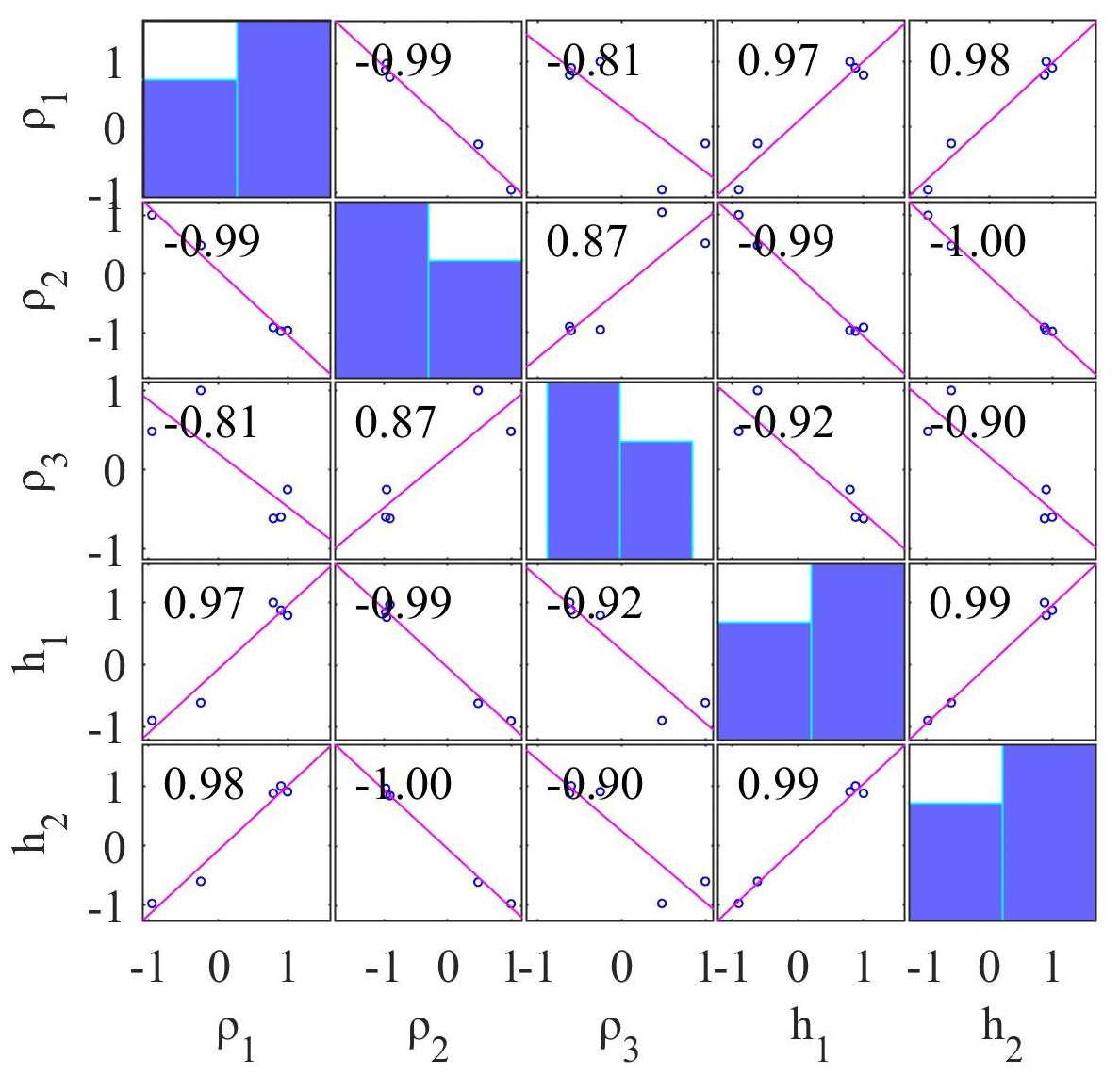
Figure 8 Correlation matrix calculated from the PSO inverted model using three-layer noise-free synthetic MT apparent resistivity and apparent phase data.

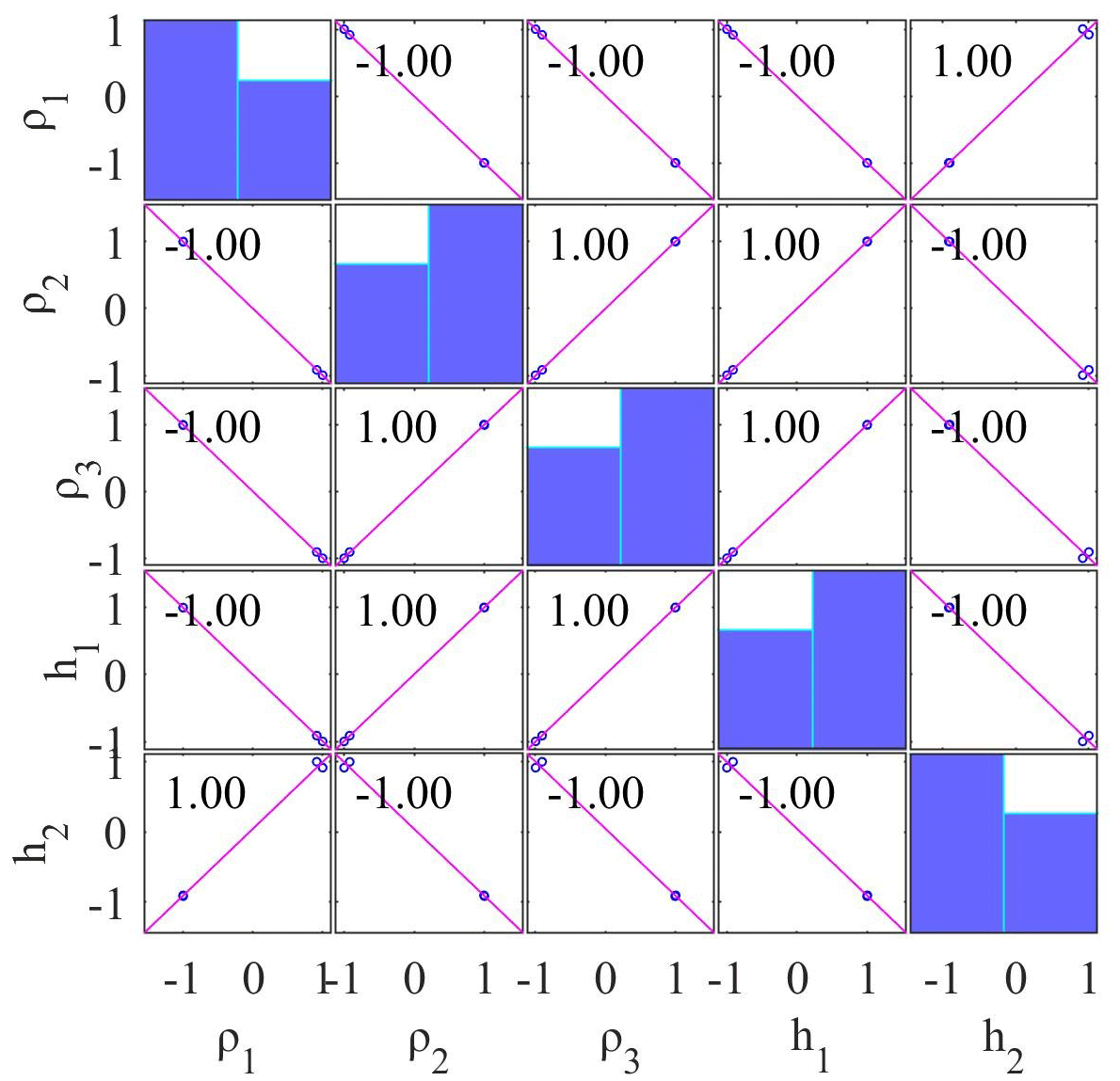
Figure 9 Correlation matrix calculated from the GSA inverted model using three-layer noise-free synthetic MT apparent resistivity and apparent phase data.

Figure 10 shows the correlation matrix of wPSOGSA. The analyses reveal that the first-layer resistivity is strongly negative with the second-layer resistivity, substantially negative (−0.92) with the third-layer resistivity, weakly positive (0.30) with the first-layer thickness, and considerably (0.63) with the second-layer thickness. Second-layer resistivity is slightly positive (0.31) when compared to third-layer resistivity (0.43) but substantially negative when compared to first-layer thickness. Third-layer resistivity has a slightly negative correlation (−0.23) with first-layer thickness but a moderately negative correlation (−0.71) with second-layer thickness, and first-layer thickness has a negative correlation (−0.71). Thus, the conclusion can be made that the layer parameters are independent of others, so changing one will have no effect on the other, compared to the result obtained via PSO and GSA.

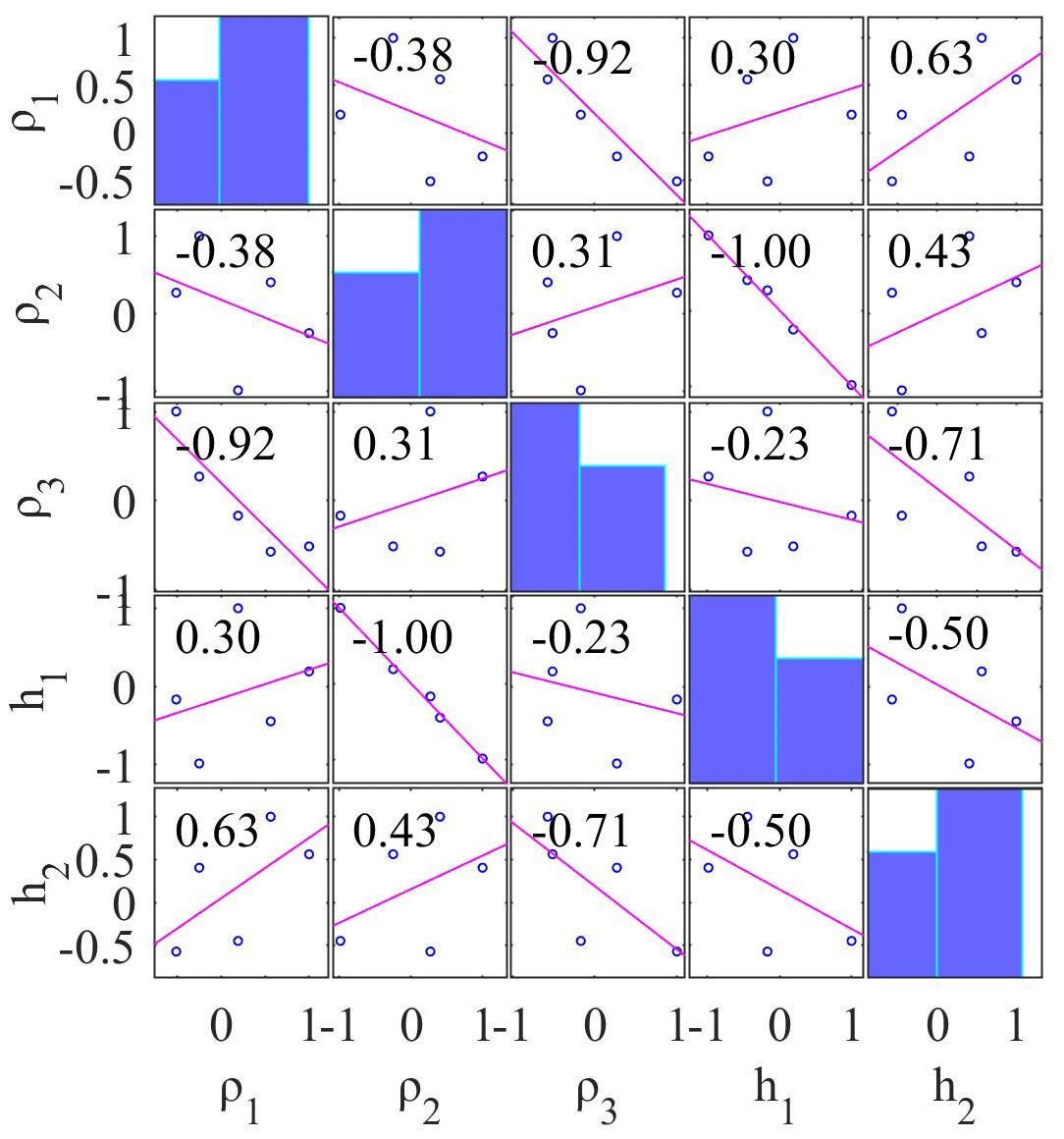
Figure 10 Correlation matrix calculated from the wPSOGSA inverted model using three-layer noise-free synthetic MT apparent resistivity and apparent phase data.

3.1.3 Stability analysis

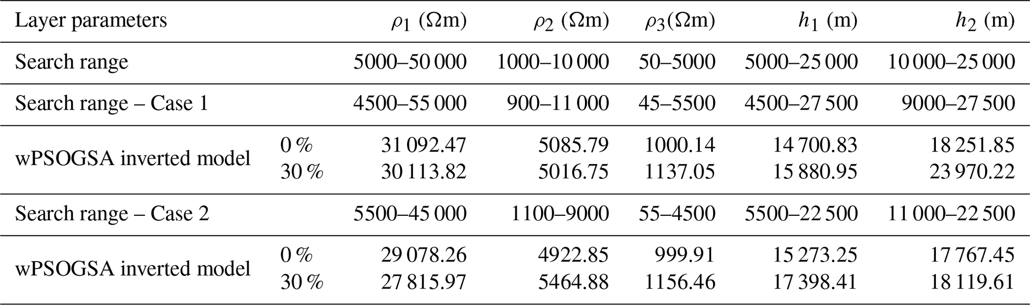
We used two different search ranges for stability evaluation of the proposed wPSOGSA and executed the algorithms over three layers of synthetic MT data, one of which is expanded, and the other is contracted by 10 % of the initial search range. We infer from three layers of synthetic data that results fluctuate by approximately 3 % from the true value when the search range is changed. This variation is about 10 % on average for synthetic data corrupted with 30 % random noise, as shown in Table 2.

Table 2 Stability analysis of a hybrid algorithm for three layers of synthetic data.

3.2 Application to synthetic MT data – four-layer case

For the second example of the synthetic data, a typical four-layer HK-type of Earth model to analyze the performance of the present algorithm with improved differential evolution (IDE) results obtained by Xiong et al. (2018). Analysis over noisy synthetic data is done by corrupting synthetic data with 10 % and 20 % Gaussian random noise to mimic the real field data because different types of noises influence apparent resistivity data. Following that, all three optimization methods are run using the noisy synthetic data. As the misfit error increases with the noise in the data, the Bayesian PDF of 68.27 % CI is calculated with respect to the threshold misfit error of 0.01, and thus the mean model is calculated.

Enormous uncertainty is shown in the inverted results; hence, we calculated the mean model for 68.27 % CI using the posterior Bayesian PDF to reduce the uncertainty and produce the global best solution. The optimized results obtained from the posterior PDF and the true model are shown in Table 3. Figure 11 illustrates that the inverted responses for PSO, GSA, and wPSOGSA are well-fitting as follows (a) observed and calculated apparent resistivity data, (b) observed and calculated apparent phase data, (c) 1-D depth model, and (d) convergence response of present algorithms. We have estimated the layer parameters for synthetic data corrupted with 20 % random noise for comparative analysis and found that PSO, GSA, and wPSOGSA converge at iterations 96, 556, and 187, with associated errors of 3.69, 4.04, and 3.69, respectively.

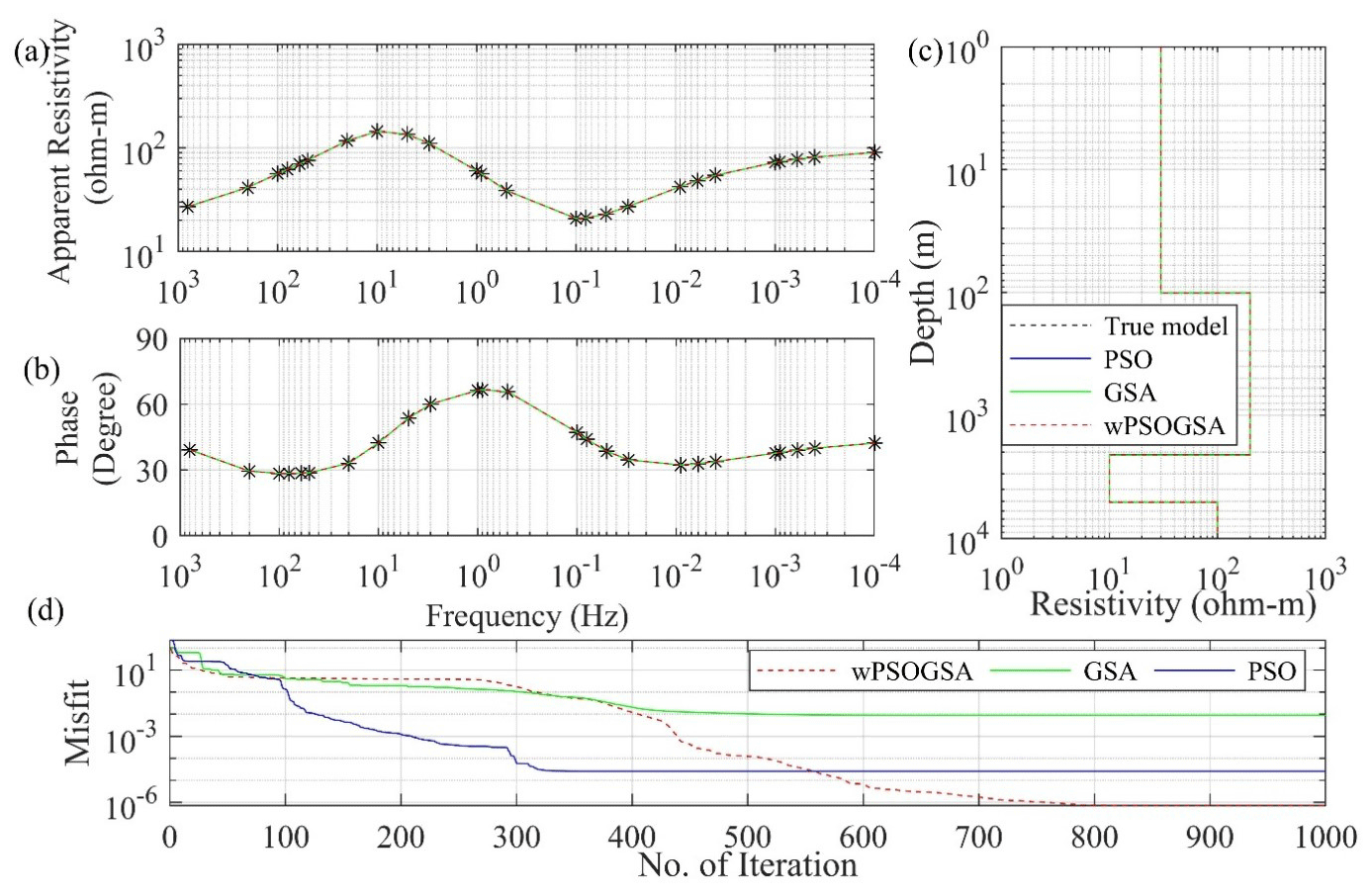
Figure 11 The inverted MT response by PSO (blue color), GSA (green color), and hybrid wPSOGSA (red color) with a true model (black color) over four-layer synthetic data as shown in (a) the observed and calculated apparent resistivity curve, (b) the observed and calculated apparent phase curve, (c) the 1D depth inverted model, and (d) the convergence curve.

Additionally, the synthetic data corrupted with 10 % random noise are also used for the execution of inversion, keeping the search range, a number of particles, and iterations the same as before; it was observed that PSO, GSA, and wPSOGSA converge at iterations 151, 2, and 250, with associated errors of 1.7609, 1.95, and 1.76, respectively. The posterior Bayesian PDF for threshold data with 68.27 % CI is calculated similarly to a three-layer case to minimize the uncertainty in inverted results.

Table 3 Comparison of the result obtained from improved differential evolution (IDE) and inverted results of PSO, GSA, and hybrid wPSOGSA obtained using the posterior PDF for four-layer synthetic apparent resistivity data with different Gauss noise levels (0 %, 10 %, and 20 %) and the true model.

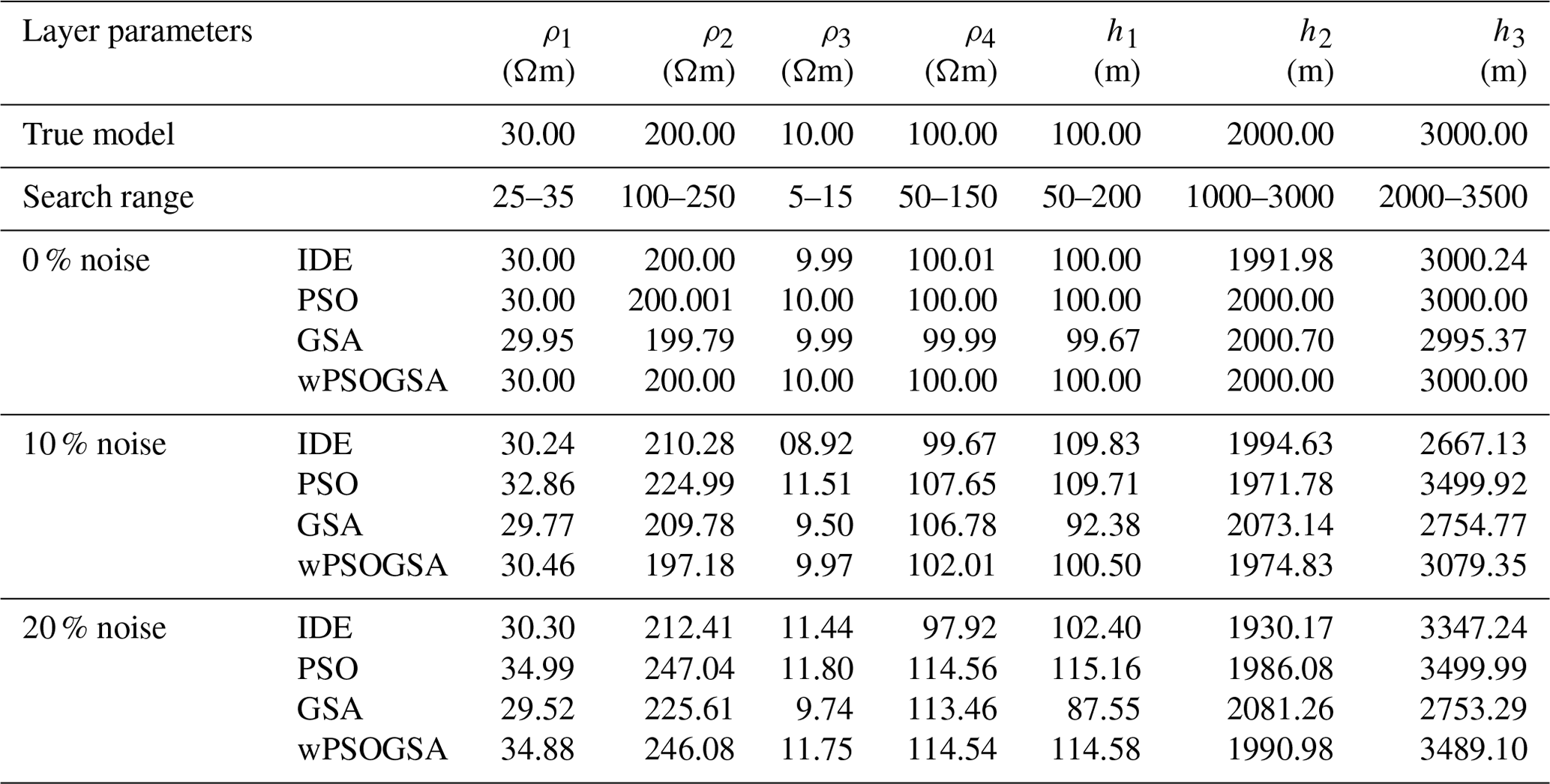
Stability analysis

For the stability evaluation of presented algorithms over four layers of synthetic MT data, similar to the three-layer case, we used two different search ranges and executed the algorithms for 1000 iterations. The method exhibits good results with four layers of synthetic data and reveals minimal variation for noise-free data. For 30 % contaminated data, the variation is approximately 10 % and 12 % in Case 1 and Case 2, respectively. The outputs do not change much across runs and provide consistent results, as shown in Table 4.

Table 4 Stability analysis of a hybrid algorithm for four layers of MT synthetic data.

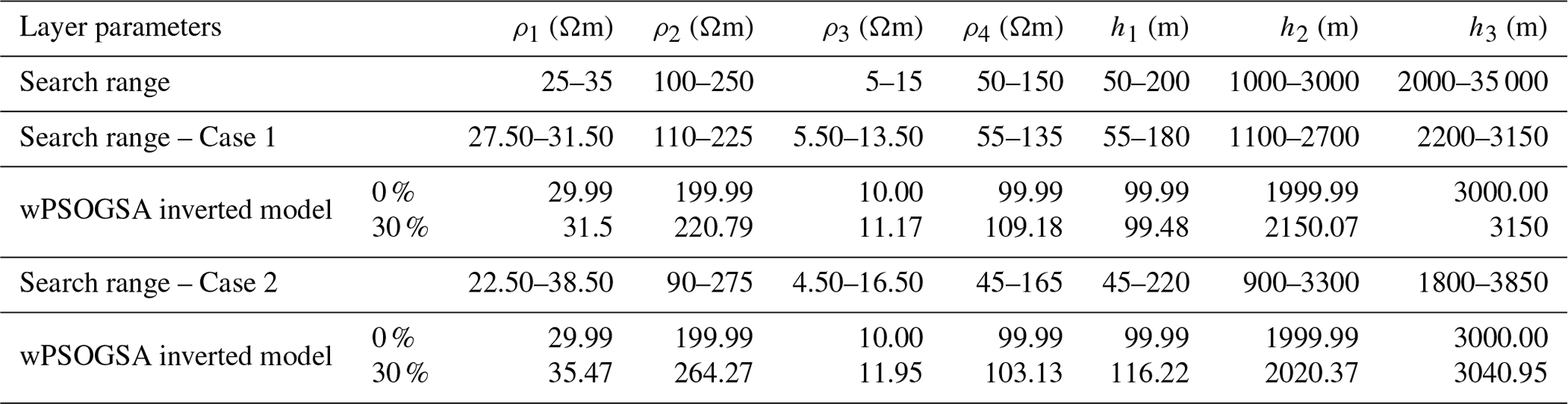
3.3 Application to field MT data – island of Milos, Greece

In one-dimensional MT data for site G5 near borehole M2 (Hutton et al., 1989), as shown in Fig. 12, the apparent resistivity and phase values are inverted using wPSOGSA, PSO, and GSA, keeping the same set of controlling parameters as for noisy synthetic data, such as the swarm size, inertia weight (w), personal learning coefficient (c₁), global learning coefficient (c₂), descending coefficient (α), and initial value of the universal gravitational constant (G₀).

Figure 12 The location of the MT site and geology of the island of Milos, Greece (after Stewart and McPhie, 2006).

Figure 13 shows the calculated data and model parameters as (a) a match between observed and computed apparent resistivity data and (b) a match between observed and computed apparent phase data; (c) the 1D inverted model; and (d) the convergence response of wPSOGSA (red color), GSA (green color), and PSO (blue color), along with the true model (black color). Figure 13c depicts alluvium deposits with a resistivity of 1.0 Ωm with 15 m thickness as the top layer, and volcanic deposits with a resistivity of 300 Ωm and 10 m thickness lie beneath the alluvium deposits. A very high conducting layer of resistivity less than 1.0 Ωm is estimated, equivalent to the green lahar under the high resistivity volcanic deposits. The next layer below, with higher resistivity, corresponds to the crystalline foundation. In the geothermal zone's depths, the resistivity drops again. The resistivity in the depth range of about 1000 m, which is similar to earlier studies, was explored, and the findings of the proposed algorithm were discovered to be in good agreement with the model developed by Dawes in Hutton et al. (1989).

Figure 13d reveals that the algorithms converge at iterations 218, 1, and 425, with corresponding errors of 0.0494, 0.0518, and 0.0493 for PSO, GSA, and wPSOGSA, respectively. The hybrid algorithm has the least error between observed and computed data. The algorithms are executed for 1000 iterations and 10 000 models, and findings are compared with available stratigraphy. The result is derived using the Monte Carlo technique by Hutton et al. (1989). After examining our optimized effects from Fig. 13 and Table 5, hybrid wPSOGSA outperformed PSO and GSA.

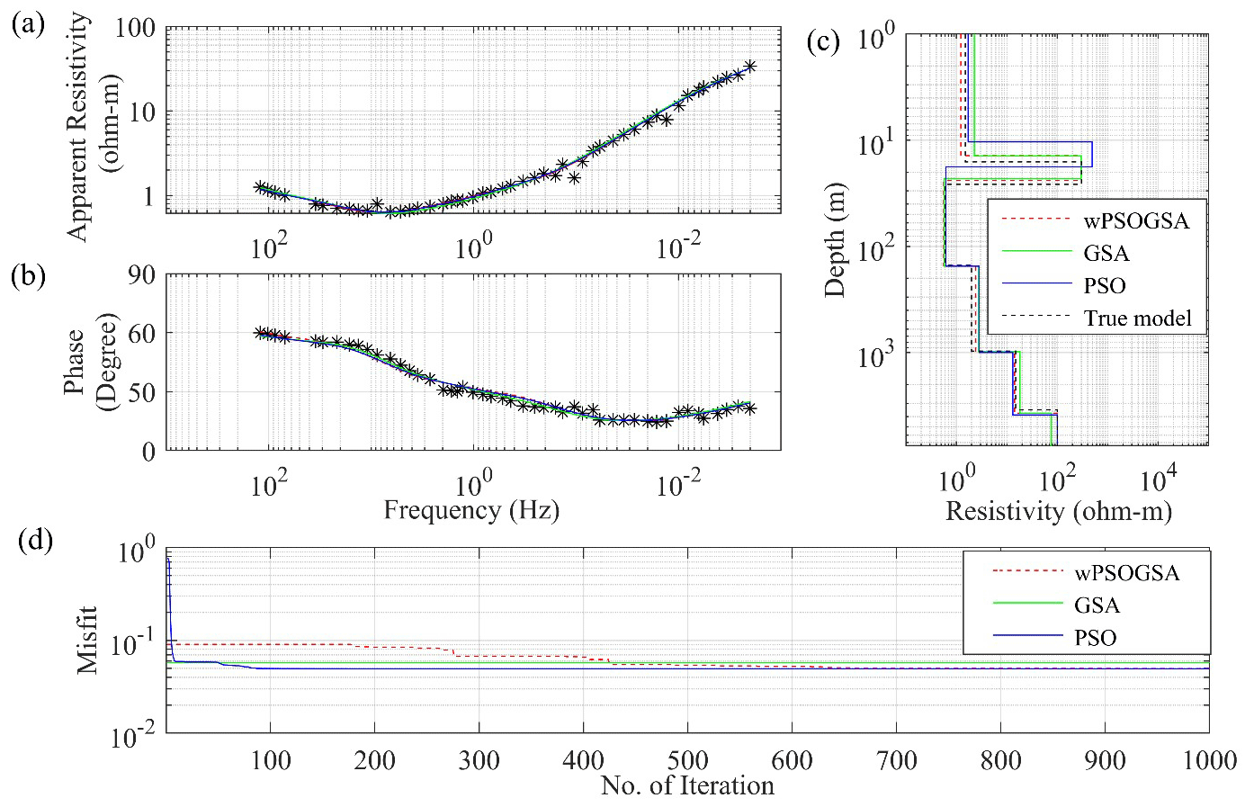
Figure 13 The inverted MT response by PSO (blue color), GSA (green color), and hybrid wPSOGSA (red color) with a true model (black color) over the geothermal area, island of Milos, Greece, as shown in (a) the observed and calculated apparent resistivity curve, (b) the observed and calculated apparent phase curve, (c) the 1D depth inverted model, and (d) the convergence curve.

3.3.1 Bayesian analysis and uncertainty in model parameters

A posterior Bayesian method determines the global model and related uncertainty. Figure 14 shows another uncertainty study that examined the six-layered resistivity model over the geothermal field, island of Milos, Greece, and found that the peak values of the posterior PDF for all model parameters are much closer to the actual value of the layer parameters, providing less uncertainty. We have analyzed the wPSOGSA inverted results from Fig. 14 and Table 5 and found that the first, second, third, fourth, fifth, and sixth layers' resistivity with uncertainty in associated layer parameters is 1.23±0.49, 297.61±53.43, 0.55±0.02, 2.41±0.16, 14.18±1.76, and 99.92±0.37 Ωm. Similarly, the associated thicknesses with uncertainty are 14.51±1.35, 9.85±1.35, 127.39±6.01, 823.01±7.57, and 2750.88±63.07 m. Thus, the analysis suggests the lower uncertainties in each layer's parameters except resistivity of the first and second layers.

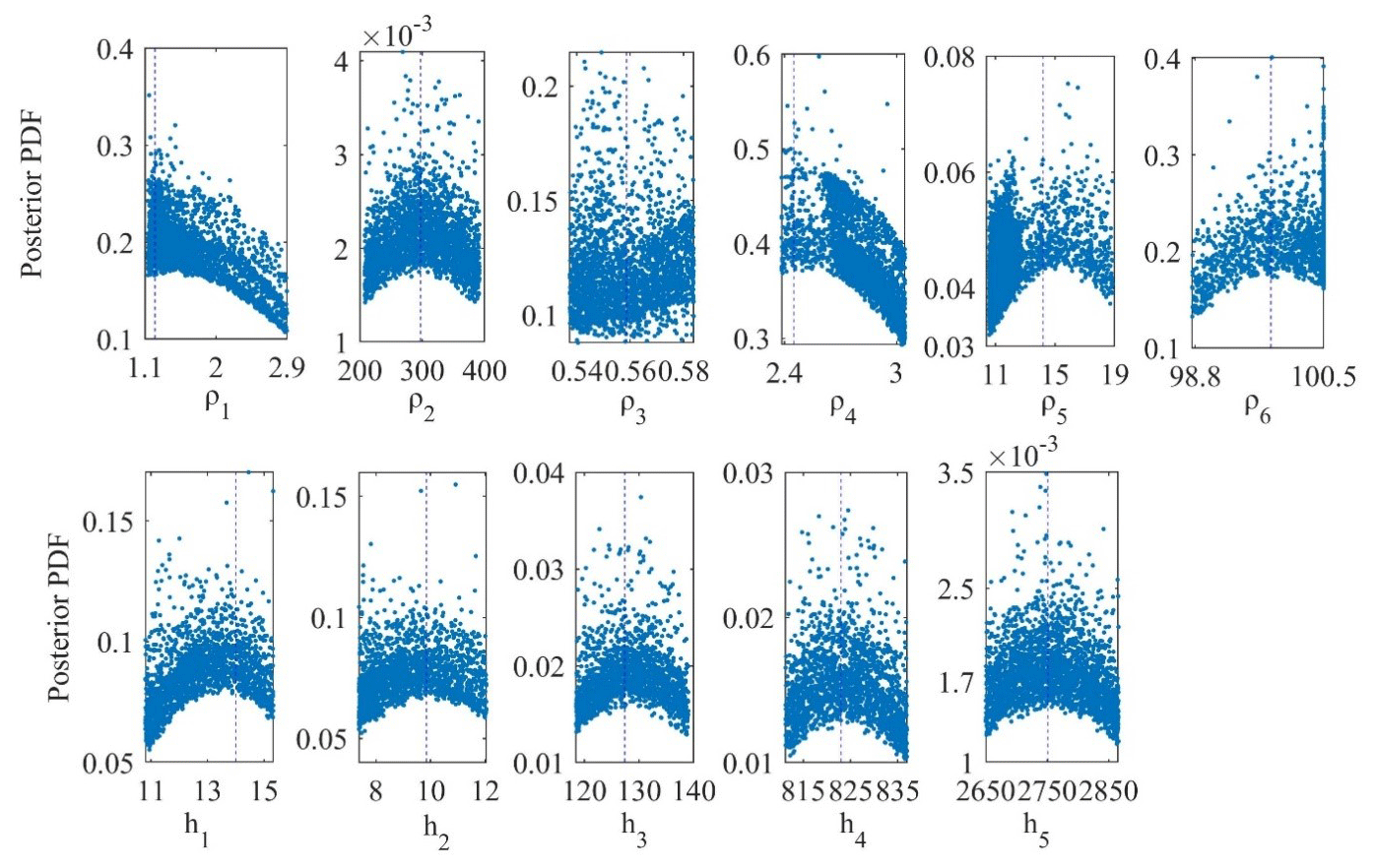
Figure 14 The posterior Bayesian probability density function (PDF) with 68.27 % CI for wPSOGSA over a geothermal field, island of Milos, Greece.

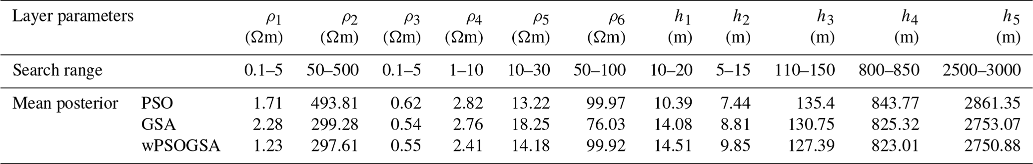
Table 5 compares optimized results obtained from all three presented algorithms based on the posterior Bayesian PDF under 68.27 % CI condition. However, the 1D depth model inverted from wPSOGSA shows good agreement with the available borehole M-2 (Hutton et al., 1989). As a result, the hybrid algorithm is functioning better, and the findings are encouraging.

Table 5 Search range and inverted results by the posterior PDF (68.27 % CI) and PSO, GSA, and hybrid wPSOGSA for six-layered field data.

3.3.2 Sensitivity, correlation matrix, and model parameters

Here, a similar study of the correlation matrix is carried out for field example from the island of Milos, Greece, using all accepted models, which have posterior PDF values within 68.27 % CI. The correlation matrix of PSO, GSA, and wPSOGSA was examined over the field MT data as shown in Figs. 15, 16, and 17, demonstrating the sensitivity among inverted model parameters, and found an almost similar correlation among the layer parameters for three-layer synthetic study. From correlation analyses, we noticed that the values are showing moderate and weak correlation among parameters in the wPSOGSA case, indicating that wPSOGSA is linearly independent of layer parameters. This indicates that the parameter is less affected by other layer parameters and resistivity curves, whereas the correlation among layer parameters for field data using GSA and PSO is either strongly positive or strongly negative, which shows that the parameters are dependent on each other. Thus a change in one parameter affects the other, and the apparent resistivity curve is also very much involved.

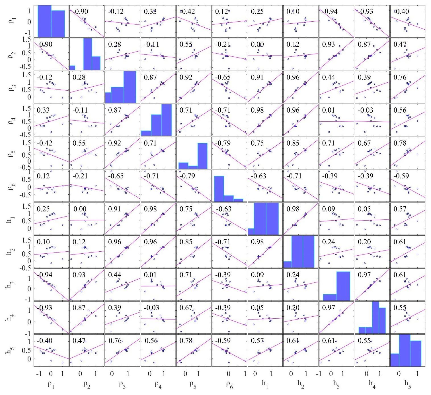
Figure 15 Correlation matrix of field data taken from the geothermally rich area of the island of Milos, Greece, for PSO.

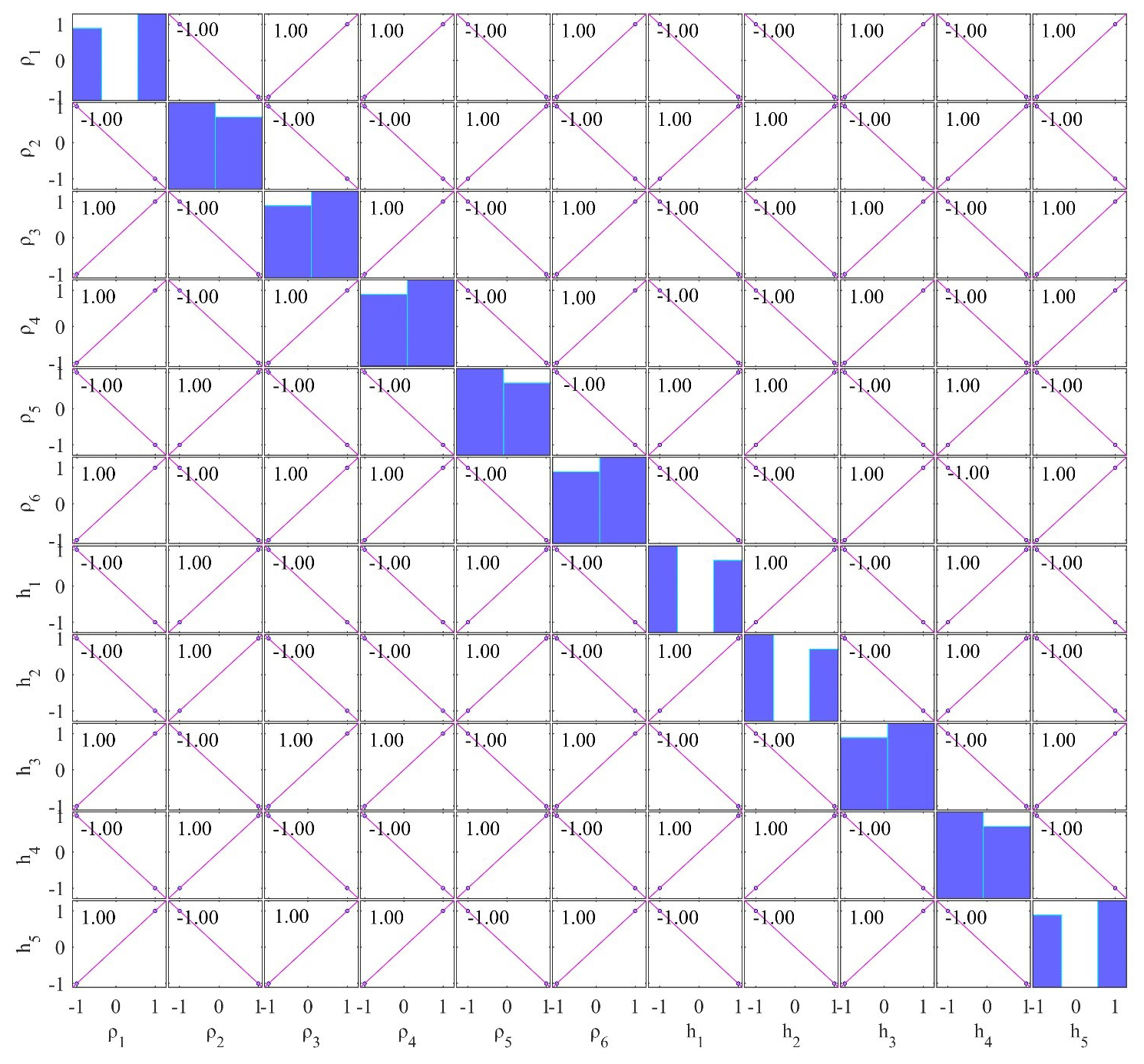
Figure 16 Correlation matrix of field data taken from the geothermally rich area of the island of Milos, Greece, for GSA.

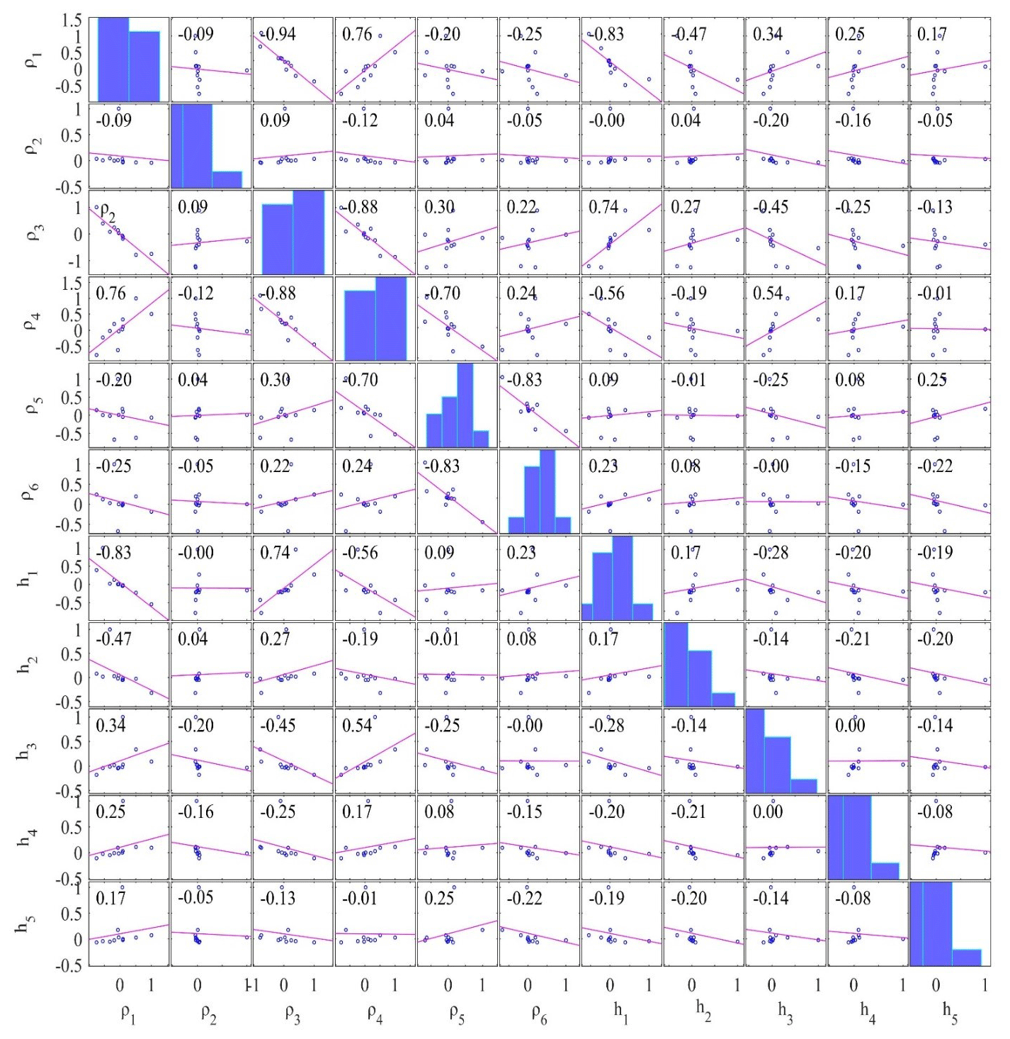
Figure 17 Correlation matrix of field data taken from the geothermally rich area of the island of Milos, Greece, for hybrid wPSOGSA.

3.4 Application to field MT data – Newcastleton, Southern Uplands, Scotland

Another field example of MT data was picked to illustrate our technique from Newcastleton (55.196^∘ N, 2.796^∘ W, in geographic coordinates), Southern Uplands of Scotland. The Southern Uplands are isolated from the Midland Valley by the Southern Uplands fault. The location of the MT site and the geology of the study area are shown in Fig. 18.

During 9 d, in the frequency range of 0.1 to 0.0001 Hz, the variations of the magnetic and telluric fields concerning the time at four sites along a line perpendicular to the anomaly's strike were recorded, keeping a high signal-to-noise ratio, where the anisotropy ratios were very near to 1, and the skew factor is less than 0.1 for the majority of periods. Due to low anisotropy ratios and the skew factor, the resistivity distribution under this location is one-dimensional (Jones and Hutton, 1979). Here one set of MT data is inverted using PSO, GSA, and wPSOGSA to obtain the best fitting apparent resistivity curve, apparent phase curve, and 1D depth model, as shown in Fig. 19a, b, and c, respectively. Figure 19 shows a realistic one-dimensional resistivity variation, with a phase response ranging from 60^∘ at 100 s to 35^∘ at 1000 s, which can only be obtained by establishing a conducting zone at lower crustal–upper mantle levels (Jones and Hutton, 1979).

The execution time for wPSOGSA (33 s) is the lowest as compared to GSA (34 s) and PSO (53 s). The convergence iterations of PSO, GSA, and wPSOGSA are 79, 101, and 65, and its associated misfit errors are 3.79, 4.72, and 3.70, respectively.

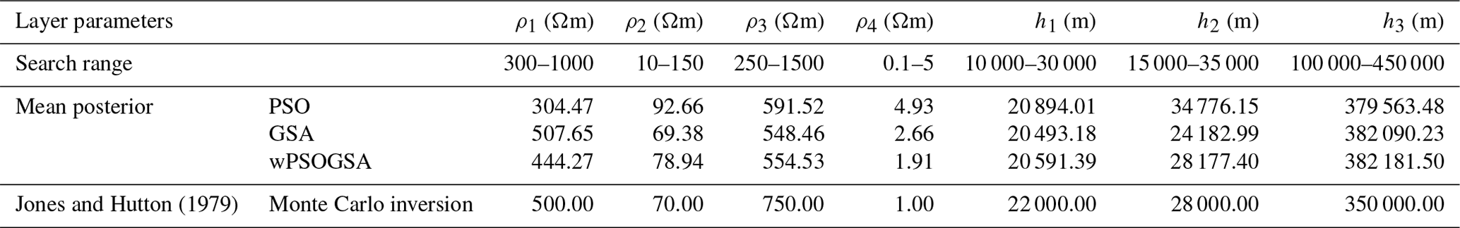
The inverted MT model is illustrated in Fig. 19c, which depicts two low conductive zones at a depth of 21 and 400 km. The first conductive layer (70 Ωm) with a thickness of 28 km is underlain by a high resistive top layer of thickness of 21 km, and the second very high conductive layer (less than 1.0 Ωm) at a depth of 400 km is underlain by a high resistive layer (550 Ωm) of thickness 351 km. Thus, the last layer of a very high conductive zone (i.e., resistivity less than 1.0 Ωm) as a lower crust–upper mantle conductor at a depth of 400 km is estimated. At 400 m depths, a conducting zone meets both the amplitude and phase long period responses. This explanation is directly equivalent to accepted models derived from Monte Carlo models for the structure underlying the Southern Uplands.

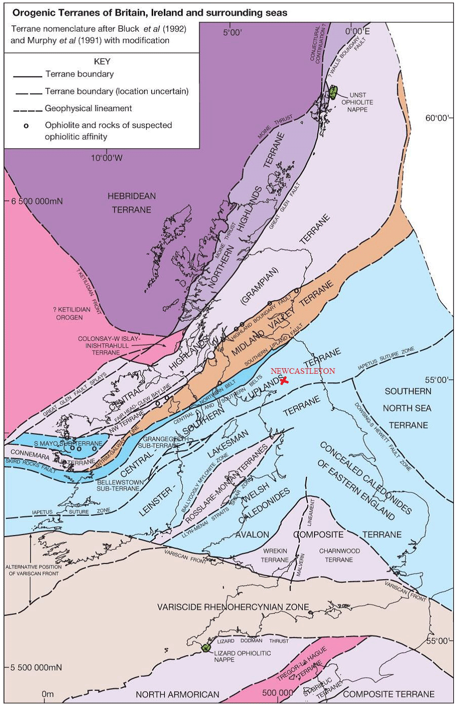
Figure 18 The location of the MT site and the geology of the Southern Uplands, Scotland (after Leslie et al., 2015).

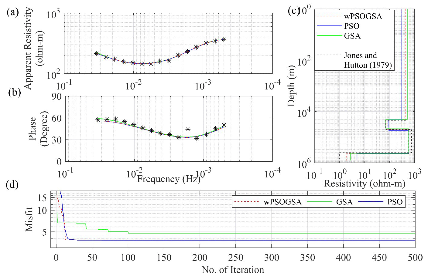
Figure 19 The inverted MT response by PSO (blue color), GSA (green color), and hybrid wPSOGSA (red color) with a true model (black color) over Newcastleton, southern Scotland, as shown in (a) the observed and calculated apparent resistivity curve, (b) the observed and calculated apparent phase curve, (c) the 1D depth inverted model, and (d) the convergence curve.

Table 6 Search range, inverted results by the posterior PDF (68.27 % CI) using PSO, GSA, and wPSOGSA for field data.

4 Discussions

The analysis on the two synthetic MT datasets shows that the proposed algorithm works very well and provides encouraging well-fitted calculated apparent resistivity and apparent phase data with the associated observed data. Also from the study, it is noted that the proposed algorithm is less sensitive to the search range and the constraints used in this algorithm. And the comparison of the model parameters shows that the output from the proposed algorithm is very precise in comparison to the true model and faster than the individual algorithms and the other algorithms used in the previous papers.

Table 7 Inverted results by the Dawes method, Jupp–Vozoff method, the Fischer inversion method (resistivity in Ωm), and Parker D+ inversion.

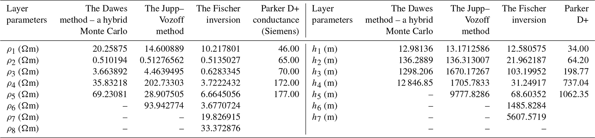
A research study conducted by Hutton et al. (1989) compared various techniques, including Parker H+, Dawes (a combined Monte Carlo–Hedgehog approach developed by Dawes), Jupp–Vozoff, Fischer, and Parker D+ inversions, to interpret the subsurface geology of the island of Milos, Greece. Among these techniques, the Dawes algorithm proved to be the most effective in identifying a reservoir interface at the borehole's depth. Consequently, these methods were utilized to compile 1-D models along several traverses. All three models, Parker H+, Parker D+, and Dawes, indicate the presence of a resistivity boundary at a depth of approximately 1000 m (Hutton et al., 1989), where the geothermal reservoir has been detected. The research findings through the proposed algorithm reveal that the resistivity of the crystalline basement beneath the geothermal site is abnormally low (<20 Ωm) in the uppermost portion and remains below 50 Ωm at depths of at least 10 km.

Figure 19c presents the inverted MT model of the Southern Uplands, Scotland, displaying two zones of low conductivity at depths of 21 and 400 km. Contrary to the findings of Jain and Wilson (1967), there is strong evidence suggesting that the conducting zone (70 Ωm) beneath the Southern Uplands exists at a depth exceeding 20 km. Furthermore, there is a second layer of extremely high conductivity (representing lower crust–upper mantle of less than 1.0 Ωm) at a depth of 400 km, which is underlain by a highly resistive layer (550 Ωm) spanning a thickness of 351 km. At a depth of 400 m, this conducting zone shows a direct alignment with both the amplitude and phase responses of long period measurements, which can be noticed in the model derived from Monte Carlo simulations of the structure underlying the Southern Uplands (see Fig. 19). The results from the proposed algorithm as well as from PSO and GSA (see Fig. 19) demonstrate the presence of a highly conductive layer at depths exceeding 20 and 400 km, corroborating the findings of Jones and Hutton (1979).

5 Conclusions

The study presented wPSOGSA along with PSO and GSA and evaluated their efficacy and applicability to the MT data. These algorithms narrate the appraisal of 1D resistivity models from apparent resistivity, apparent phase, and frequency datasets. So, synthetic and field MT data from various geological terrains were used to demonstrate the relevance of these methods, which are further carried out by applying multiple runs, generating a large number of models that fit the apparent resistivity and apparent phase curves. Furthermore, these best-fitting models within a specified range are then chosen for statistical analysis. The statistical analysis includes the posterior PDF based on the Bayesian approach with a 68.27 % CI, the correlation matrix, and stability analysis in order to understand the accuracy of the mean model and its uncertainty. However, the solution from the posterior PDF based on the Bayesian of wPSOGSA is better than GSA and PSO, explaining the reliability of the proposed inversion algorithm. In general, conventional techniques can effectively resolve the model in random noise, but they can miscarry in methodical error or inappropriate models. Also, the performance of the proposed algorithms on field datasets has been analyzed based on the mean model, uncertainty, correlation, and stability of layered Earth models, and it was found that the results obtained from wPSOGSA are reliable, stable, and more accurate than the available results, which are well adapted to borehole lithology.