the Creative Commons Attribution 4.0 License.
the Creative Commons Attribution 4.0 License.
 | 16 Aug 2023
Review article: Scaling, dynamical regimes, and stratification. How long does weather last? How big is a cloud?
Until the 1980s, scaling notions were restricted to self-similar homogeneous special cases. I review developments over the last decades, especially in multifractals and generalized scale invariance (GSI). The former is necessary for characterizing and modelling strongly intermittent scaling processes, while the GSI formalism extends scaling to strongly anisotropic (especially stratified) systems. Both of these generalizations are necessary for atmospheric applications. The theory and some of the now burgeoning empirical evidence in its favour are reviewed.
Scaling can now be understood as a very general symmetry principle. It is needed to clarify and quantify the notion of dynamical regimes. In addition to the weather and climate, there is an intermediate “macroweather regime”, and at timescales beyond the climate regime (up to Milankovitch scales), there is a macroclimate and megaclimate regime. By objectively distinguishing weather from macroweather, it answers the question “how long does weather last?”. Dealing with anisotropic scaling systems – notably atmospheric stratification – requires new (non-Euclidean) definitions of the notion of scale itself. These are needed to answer the question “how big is a cloud?”. In anisotropic scaling systems, morphologies of structures change systematically with scale even though there is no characteristic size. GSI shows that it is unwarranted to infer dynamical processes or mechanisms from morphology.
Two “sticking points” preventing more widespread acceptance of the scaling paradigm are also discussed. The first is an often implicit phenomenological “scalebounded” thinking that postulates a priori the existence of new mechanisms, processes every factor of 2 or so in scale. The second obstacle is the reluctance to abandon isotropic theories of turbulence and accept that the atmosphere's scaling is anisotropic. Indeed, there currently appears to be no empirical evidence that the turbulence in any atmospheric field is isotropic.
Most atmospheric scientists rely on general circulation models, and these are scaling – they inherited the symmetry from the (scaling) primitive equations upon which they are built. Therefore, the real consequence of ignoring wide-range scaling is that it blinds us to alternative scaling approaches to macroweather and climate – especially to new models for long-range forecasts and to new scaling approaches to climate projections. Such stochastic alternatives are increasingly needed, notably to reduce uncertainties in climate projections to the year 2100.
- Article
(59611 KB) - Full-text XML
- BibTeX
- EndNote


1.1 Dynamical ranges, fluctuations, and scales
Perhaps the most obvious difficulty in understanding the atmosphere is in dealing with its enormous range of scales. The single picture in Fig. 1 shows clouds with horizontal spatial variability ranging from millimetres to the size of the planet, a factor of 10 billion in scale. In the vertical direction the range is more modest but still huge: about 10 million. The range of temporal variability is extreme, spanning a range of 100 billion billion: from milliseconds to the planet's age (Fig. 2).
The earliest approach to atmospheric variability was phenomenological: weather as a juxtaposition of various processes with characteristic morphologies, air masses, fronts, and the like. Circumscribed by the poor quality and quantity of the then available data, these were naturally associated with narrow-scale-range, mechanistic processes.
At first, ice ages, “medieval warming”, and other evidence of low-frequency processes were only vaguely discerned. Weather processes were thought to occur with respect to a relatively constant (and unimportant) background: climate was conceived as simply long-term “average” weather. It was not until the 1930s that the International Meteorological Organisation defined “climate normals” in an attempt to quantify the background “climate state”. The duration of the normals – 30 years – was imposed essentially by fiat: it conveniently corresponded to the length of high-quality data then available: 1900–1930. This 30-year duration is still with us today with the implicit consequence that – purely by convention – “climate change” occurs at scales longer than 30 years.
Interestingly, yet another official timescale for defining “anomalies” has been developed. Again, for reasons of convenience (and partly – for temperatures – due to the difficulty in making absolute measurements), anomalies are defined with respect to monthly averages. Ironically, a month wavers between 28 and 31 d: it is not even a well-defined unit of time.
The overall consequence of adopting, by convenience, monthly and 30-year timescales is a poorly theorized, inadequately justified division of atmospheric processes into three regimes: scales less than a month, a month up to 30 years, and a lumping together of all slower processes with timescales longer than 30 years. While the high-frequency regime is clearly “weather” and the slow processes – at least up to ice age scales – are “climate”, until Lovejoy (2013) the intermediate regime lacked even a name. Using scaling – and with somewhat different transition scales – the three regimes were finally put on an objective quantitative basis, with the middle regime baptized “macroweather”. By using scaling to quantitatively define weather, macroweather, and climate, we can finally objectively answer the question: how long does weather last? A bonus, detailed in Sect. 2, is that scaling analyses showed that what had hitherto been considered simply climate is itself composed of three distinct dynamical regimes. Rather than lumping all low frequencies together, we must also distinguish between macroclimate and megaclimate.
To review how scaling defines dynamical regimes, let us define scaling using fluctuations – for example of the temperature or of a component of the wind. For the moment, consider only one dimension, i.e. time series or spatial transects. Temporal scaling means that the amplitudes of fluctuations are proportional to their timescale raised to a scale-invariant exponent. For appropriately nondimensionalized quantities,
Every term in this equation needs an appropriate definition, but for now, consider the classical ones. First, the usual turbulence definition of a fluctuation is a difference (of temperature, wind components, etc.) taken over an interval in space or in time. This interval defines the timescale (Δt) or space scale (Δx) of the corresponding fluctuation. Also, classically, one considers the statistically averaged fluctuation (indicated by “〈〉”). If we decompose ζ into a random singularity γ and a non-random “fluctuation exponent” H, then the appropriately averaged fluctuation will also be scaling with
where the symbol 〈〉 indicates statistical (ensemble) averaging.
Later, in Sect. 2.5, fluctuations as differences (sometimes called “poor man's wavelets”) are replaced by (nearly as simple) Haar fluctuations based on Haar wavelets (see also Appendix B) and in Sect. 3, and Eq. (1) is interpreted stochastically. Finally, in Sect. 4, the notion of scale itself is generalized by introducing a scale function that replaces the usual (Euclidean) distance function (metric). These anisotropic-scale functions are needed to handle scale in 2D or higher spaces, especially with regard to stratification.
In atmospheric regimes where Eq. (1) holds, average fluctuations over durations λΔt are λH times those at duration Δt; i.e. they differ only in their amplitudes, they are qualitatively of the same nature, and they are therefore part of the same dynamical regime. More generally (Eq. 1), appropriately rescaled probabilities of random fluctuations also have scale-invariant exponents (“codimensions”, Sect. 3), so that the entire statistical behaviour is scaling. Scaling therefore allows us to objectively identify the different atmospheric regimes.
Over the Phanerozoic eon (the last 540 Myr), the five scaling regimes are weather, macroweather, climate, macroclimate, and megaclimate (Lovejoy, 2015). Starting at around a millisecond (the dissipation time), this covers a total range of ≈ 1019 in scale (Sect. 2.5; Tuck (2022) argues that the true dissipation scale is much smaller: molecular scales). Scaling therefore gives an unequivocal answer to the question posed in the title: “How long does weather last?”. The answer is the lifetime of planetary structures, typically around 10 d (Sect. 2.6).
If the key statistical characteristics of the atmosphere at any given scale are determined by processes acting over wide ranges of scales – and not by a plethora of narrow-range ones – then we must conclude that the fundamental dynamical processes are in fact dynamical “regimes” – not uninteresting “backgrounds”. While there may also be narrow-range processes, they can only be properly understood in the context of the dynamical regime in which they operate, and in any event, spectral or other analysis shows that they generally contribute only marginally to the overall variability. The first task is therefore to define and understand the dynamical regimes and then – when necessary – the narrow-range processes occurring within them.
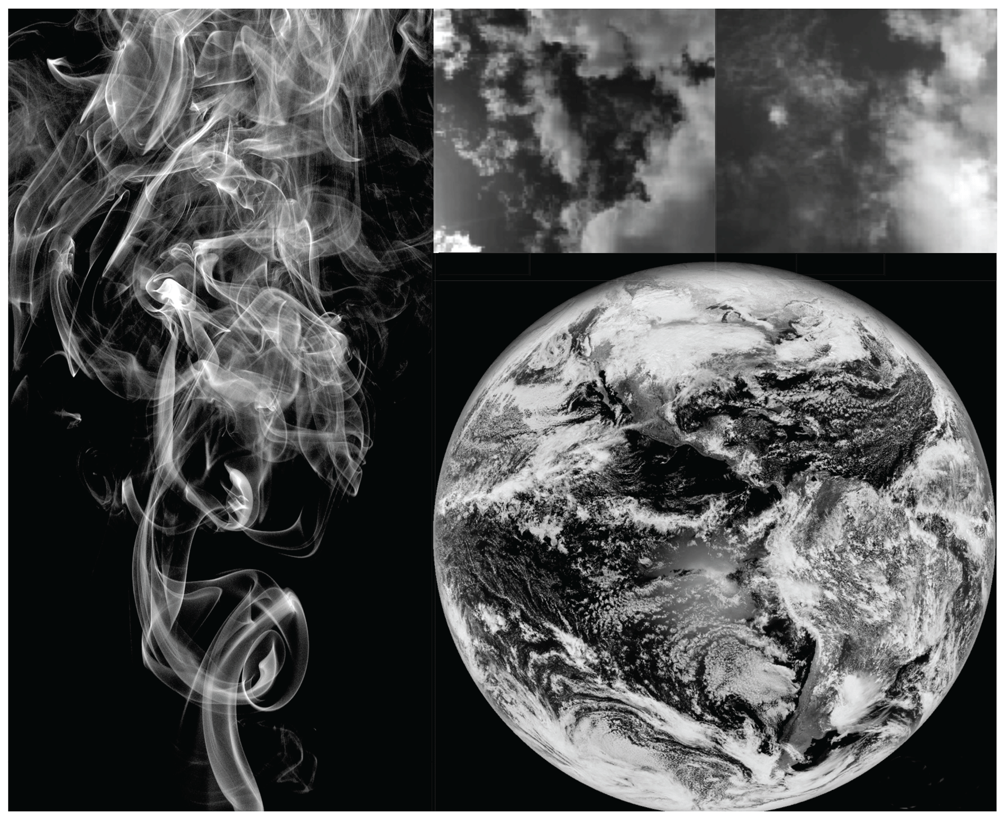
Figure 1Cigarette smoke (left) showing wisps and filaments smaller than 1 mm up to about 1 m in overall size. The upper right shows two clouds, each several kilometres across with resolutions of 1 m or so. The lower right shows the global-scale arrangement of clouds taken from an infrared satellite image of the Earth with a resolution of several kilometres. Taken together, the three images span a range of several billion in spatial scale. Reproduced from Lovejoy (2019).
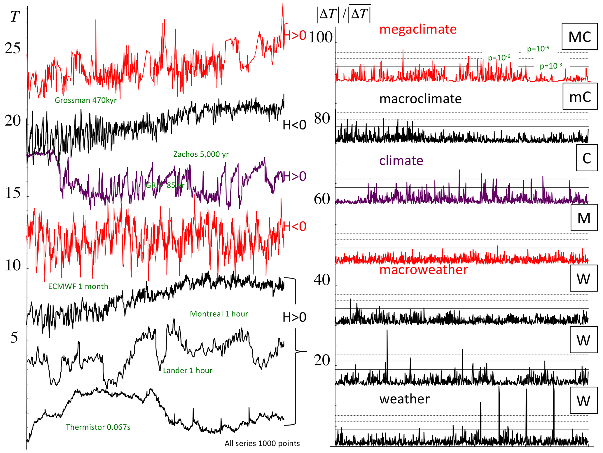
Figure 2Left: 1000 points of various time series collectively spanning the range of scales of 470 Myr to 0.067 s = 2.4 × 10¹⁷; each series was normalized so as to have the same overall range and offset in the vertical for clarity. The right-hand-side column shows the absolute first differences normalized by the mean. The solid horizontal line shows the maximum value expected for Gaussian variables (), and the dashed lines show the corresponding , 10−9 probability levels. Representative series from each of the five scaling regimes were taken with the addition of the hourly surface temperatures from Lander, Wyoming (bottom, detrended daily and annually). The Berkeley series was taken from a fairly well-estimated period before significant anthropogenic effects and was annually detrended. The top was taken over a particularly data-rich epoch, but there are still traces of the interpolation needed to produce a series at a uniform resolution. The resolutions (indicated) were adjusted so that, as much as possible, the smallest scale was at the inner scale of the regime indicated. In the macroclimate regime, the inner scale was a bit too small and the series length a bit too long. The resulting megaclimate regime influence on the low frequencies was therefore removed using a linear trend of 0.25 δ18O Myr−1. The resolutions and time periods are indicated next to the curves. The black curves have H>0 and the red ones H<0: see the parameter estimates in Appendix A. The figure is from Lovejoy (2018), updated only in the top megaclimate series that is at a higher resolution than the previous one (from Grossman and Joachimski, 2022).
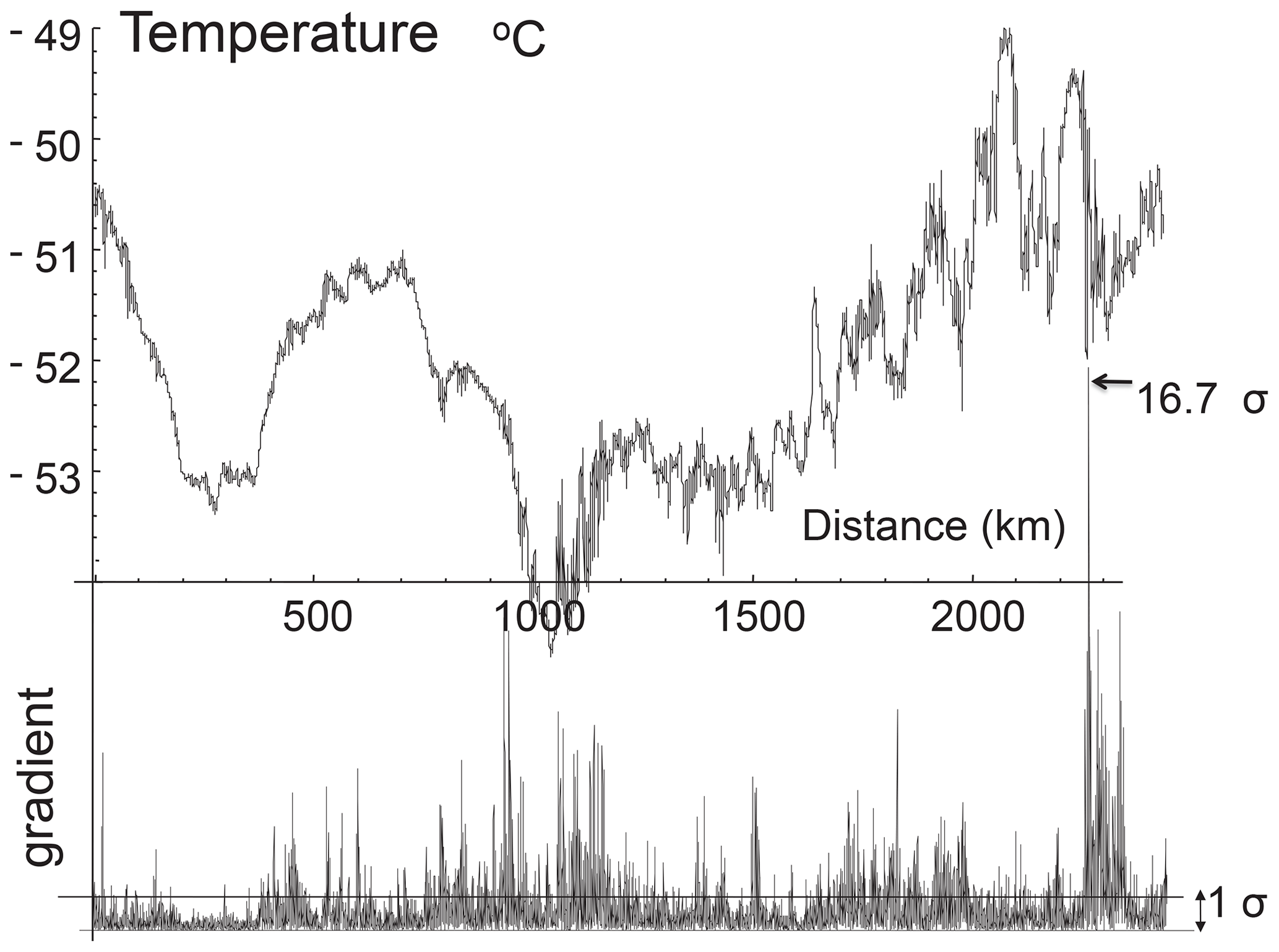
Figure 3The first 8196 points of the temperature series measured by a GulfStream 4 flight over the Pacific Ocean at 196 mb and 1 s resolution (corresponding to 280 m). Because the aircraft speed is much greater than the wind, this can be considered a spatial transect. The bottom shows the absolute change in temperature from one measurement to the next normalized by dividing by the typical change (the standard deviation). This differs from the spike plot on the right-hand side of Fig. 2 only in the normalization, here by the standard deviation, not by the absolute difference. Reproduced from Lovejoy and Schertzer (2013).
1.2 A multiscaling/multifractal complication
Before answering the quite different scaling question “How big is a cloud?”, it is first necessary to discuss a complication: that the scaling is different for every level of activity. It turns out that the wide range over which the variability occurs is only one of its aspects: even at fixed scales, the variability is much more extreme than is commonly believed. Interestingly, the extremeness of the variability at a fixed scale is a consequence of the wide range of scaling itself: it allows the variability to build up scale by scale in a multiplicative cascade manner. As a result, mathematically, the scaling of the average fluctuation (Eq. 2) gives only a partial view of the variability, and we need to consider Eq. (1) in its full stochastic sense. In particular, if the exponent ζ is random, then it is easy to imagine that the variability may be huge.
To graphically see this, it is sufficient to produce a “spike plot” (the right-hand-side columns of Fig. 2, time, and the corresponding spatial plot, Fig. 3). These spike plots are simply the absolute first differences in the values normalized by their overall means (in Fig. 3, the normalization is slightly different, by the standard deviation). In the right-hand-side column of Fig. 2 and the bottom of Fig. 3, we see – with a single but significant exception, macroweather in time (Fig. 2) – that they all have strong spikes signalling sharp transitions. In turbulence jargon, the series are highly “intermittent”.
How strong are the spikes? Using classical (Gaussian) statistics, we may use probability levels to quantify them. For example, Fig. 2 (right) shows solid horizontal lines that indicate the maximum spike that would be expected from a Gaussian process with the given number of spikes. For the 1000 points in each series in Fig. 2, this line thus corresponds to a Gaussian probability . In addition, horizontal dashed lines show spikes at levels and . Again, with the exception of macroweather, we see that the level is exceeded in every series and that the megaclimate, climate, and weather regimes are particularly intermittent, with spikes exceeding the levels. In Sect. 3 we show how the spikes can be tamed by multifractal theory and the maxima predicted reasonably accurately (Appendix A) by simply characterizing the statistics of the process near the mean (i.e. using their non-extreme behaviour).
The spikes visually underline the fact that variability is not simply a question of the range of scales that are involved: at any given scale, variability can be strong or weak. In addition, events can be highly clustered, with strong ones embedded inside weak ones and even stronger ones inside strong ones in a fractal pattern repeating to smaller and smaller scales. This fractal sparseness itself can itself become more and more accentuated for the more and more extreme events/regions: the series will generally be multifractal.
1.3 How big is a cloud?
Scaling is also needed to answer the question “how big is a cloud?” (here “cloud” is taken as a catch-all term meaning an atmospheric structure or eddy). Now the problem is what we mean by “scale”. The series and transects in Figs. 2 and 3 are 1D, so that it is sufficient to define the scale of a fluctuation by the duration (time) or length (space) over which it occurs (actually, time involves causality, so that the sign of Δt is important; see Marsan et al. (1996): we ignore this issue here). However, the state of the atmosphere is mathematically represented by fields in 3D space evolving in time.
Consider Fig. 4, which displays a cloud vertical cross section from the CloudSat radar. In the figure, the gravitationally induced stratification is striking, and since each pixel in the figure has a horizontal resolution of 1 km but a vertical resolution of 250 m, the actual stratification is 4 times stronger than it appears. What is this cloud's scale? If we use the usual Euclidean distance to determine the scale, should we measure it in the horizontal or vertical direction? In this case, is the cloud scale its width (200 km) or its height (only ≈ 10 km)?
If the horizontal–vertical aspect ratio were the same for all clouds, the two choices would be identical to within a constant factor, and the anisotropy would be “trivial”. The trouble is that the aspect ratio itself turns out to be a strong power-law function of (either) horizontal or vertical scale, so that, for any cloud,
In Sect. 4, we will see that, theoretically, the stratification exponent is , a value that we confirm empirically on various atmospheric fields, including clouds.
To further appreciate the issue, consider the simulation in Fig. 5 that shows a vertical cross section of a multifractal cloud liquid water density field. The left-hand-side column (top to bottom) shows a series of blow-ups in an isotropic (“self-similar”) cloud. Moving from top to bottom, blow-ups of the central regions by successive factors of 2.9 are displayed. In order for the cross sections to maintain a constant 50 % “cloud cover”, the density threshold distinguishing the cloud (white or grey) from the non-cloud (black) must be systematically adjusted to account for this change in resolution. This systematic readjustment of the threshold is required due to the multifractality, and with this adjustment, we see that the cross sections are self-similar; i.e. they look the same at all scales.
The effect of differential (scale-dependent) stratification is revealed in the right-hand-side column that shows the analogous zoom through an anisotropic multifractal simulation with a stratification exponent . The low-resolution (top) view of the simulation is highly stratified in the horizontal. Now, the blow-ups reveal progressively more and more roundish structures. Eventually – with the bottom cross section (a blow-up of a total factor of ≈ 5000) – we can start to see vertically oriented structures “dangling” below more roundish ones.
In the isotropic simulations (left-hand side), the only difficulty in defining the size of the cloud is the multifractal problem of deciding, for each resolution, which threshold should be used to distinguish cloud from no cloud. However, in the more realistic anisotropic simulation on the right, there is an additional difficulty in answering the question of “how big is a cloud?” Should we use the horizontal or vertical cloud extent? It turns out (in Sect. 4) that, to ensure that the answer is well defined, we need a new notion of scale itself: generalized scale invariance (GSI).
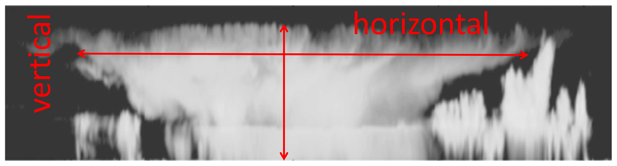
Figure 4A vertical cloud cross section of radar backscatter taken by the radar on the CloudSat satellite with resolutions of 250 m in the vertical and 1 km in the horizontal. The black areas are those whose radar reflectivities are below the radar's minimum detectable signal. The arrows show rough estimates of the horizontal and vertical extents of the cloud. The two differ by a factor of more than 10. How do they characterize the size of this cloud? Adapted from Lovejoy et al. (2009b).
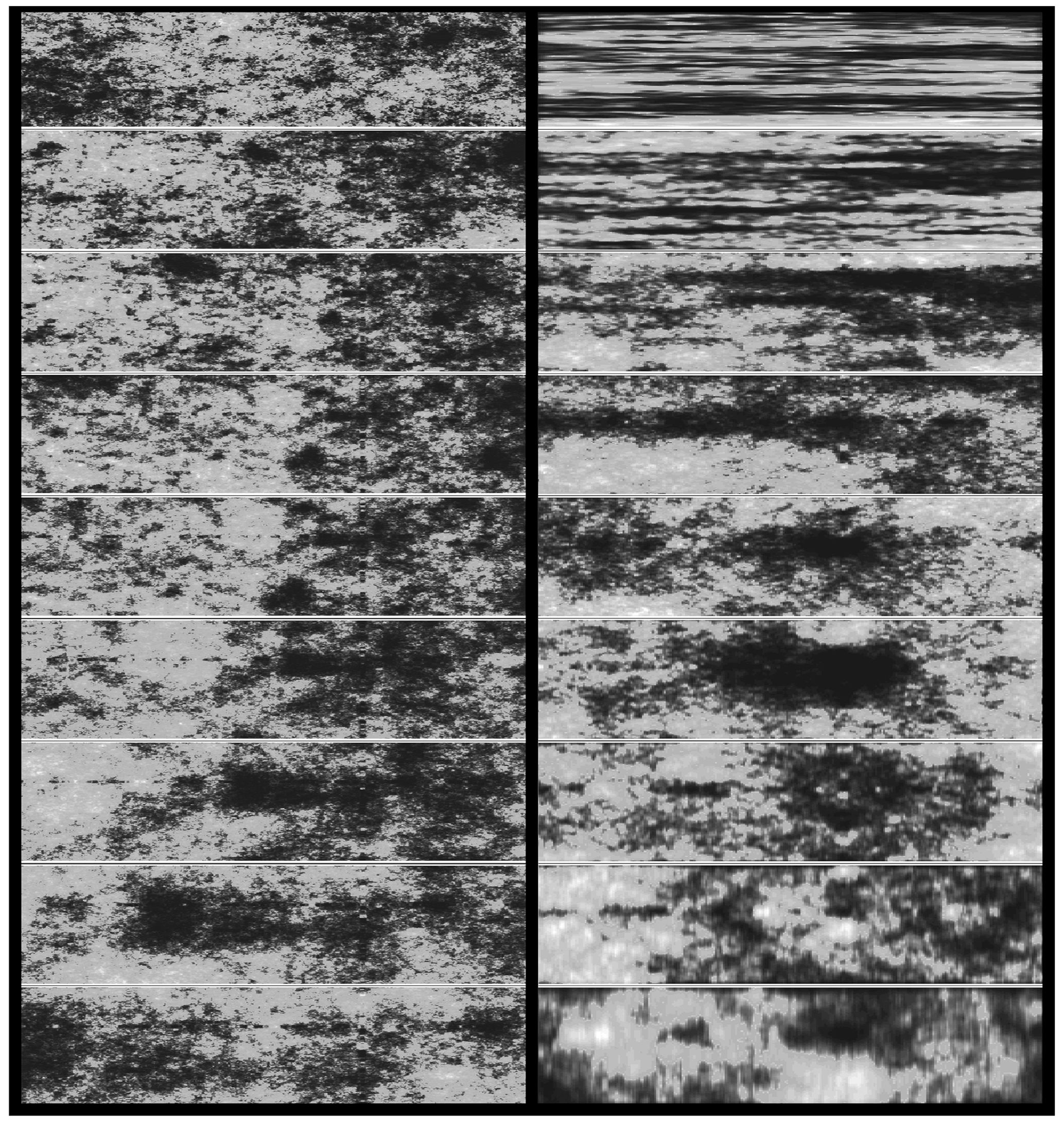
Figure 5Left column: a sequence “zooming” into a vertical cross section of an isotropic multifractal cloud (the density of liquid water was simulated and then displayed using false colours with a grey sky below a low threshold). From top to bottom, we progressively zoom in by a factor of 2.9 (total factor ≈ 1000). We can see that typical cloud structures are self-similar. In the right-hand-side column, a multifractal cloud with the same statistical parameters as on the left, but anisotropic, the zoom is still by factors of 2.9 in the horizontal, but the structures are progressively “squashed” in the horizontal. Note that while at large scales the clouds are strongly horizontally stratified, when viewed close up they show structures in the opposite direction. The spheroscale is equal to the vertical scale in the right-most simulation in the bottom row. The film version of this and other anisotropic space–time multifractal simulations can be found at http://www.physics.mcgill.ca/~gang/multifrac/index.htm, last access: 14 July 2023). This is reproduced from Blöschl et al. (2015).
1.4 Wide-range scaling and the scalebound and isotropic turbulence alternatives
1.4.1 Comparison with narrow-scale-range, “scalebound” approaches
The presentation and emphasis of this review reflect experience over the last years that has shown how difficult it is to shake traditional ways of thinking. In particular, traditional mechanistic meteorological approaches are based on a widely internalized but largely unexamined “scalebound” view that prevents scaling from being taken as seriously as it must be. As we will see (Sect. 2), the scalebound view persists in spite of its increasing divorce from the real world. Such a persistent divorce is only possible because practising atmospheric scientists rely almost exclusively on numerical weather prediction (NWP) or global circulation models (GCMs), and these inherit the scaling symmetry from the atmosphere's primitive equations upon which they are built.
The problem with scaleboundedness is not so much that it does not fit the facts, but rather that it blinds us to promising alternative scaling approaches. New approaches are urgently needed. As argued in Lovejoy (2022a), climate projections based on GCMs are reaching diminishing returns, with the latest IPCC AR6 (Arias, Bellouin et al., 2021) uncertainty ranges larger than ever before: cf. the latest climate sensitivity range of 2–5.5 K rise in global temperature following a CO2 doubling. This is currently more than double the range of expert judgement: (2.5–4 K). New low-uncertainty approaches are thus needed, and scaling approaches based on direct stochastic scaling macroweather models are promising (Hébert et al., 2021b; Procyk et al., 2022).
1.4.2 “Scaling-primary” versus “isotropy-primary” turbulence approaches
There are also sticking points whose origin is in the other, statistical, turbulence strand of atmospheric science. Historically, turbulence theories have been built around two statistical symmetries: a scale symmetry (scaling) and a direction symmetry (isotropy). While these two are conceptually quite distinct, even today, they are almost invariably considered together in the special case called “self-similarity”, which is a basic assumption of theories and models of isotropic 2D and isotropic 3D turbulence. Formalizing scaling as a (nonclassical) symmetry principle clarifies the distinct nature of scale and direction symmetries. In the atmosphere, due to gravity (not to mention sources of differential rotation), there is no reason to assume that the scale symmetry is an isotropic one: indeed, atmospheric scaling is fundamentally anisotropic. The main unfortunate consequence of assuming isotropy is that it implies an otherwise unmotivated (and unobserved) scale break somewhere near the scale height (≈ 7.4 km).
As we show (Sect. 4), scaling accounts for both the stratification that systematically increases with scale as well as its intermittency. Taking into account gravity in the governing equations provides an anisotropic scaling alternative to quasi-geostrophic turbulence (“fractional vorticity equations”; see Schertzer et al., 2012). The argument in this review is thus that scaling is the primary scale symmetry: it takes precedence over other scale symmetries such as isotropy. Indeed, it seems that isotropic turbulence is simply not relevant in the atmosphere (Lovejoy et al., 2007).
1.5 The scope and structure of this review
This review primarily covers scaling research over the last 4 decades, especially multifractals, generalized scale invariance, and their now extensive empirical validations. This work involved theoretical and technical advances, revolutions in computing power, the development of new data analysis techniques, and the systematic exploitation of mushrooming quantities of geodata. The basic work has already been the subject of several reviews (Lovejoy and Schertzer, 2010c, 2012b), but especially a monograph (Lovejoy and Schertzer, 2013). Although a book covering some of the subsequent developments was published more recently (Lovejoy, 2019), it was nontechnical, so that this new review brings its first four chapters up to date and includes some of the theory and mathematics that were deliberately omitted so as to render the material more accessible. The last three chapters of Lovejoy (2019) focused on developments in the climate-scale (and lower-frequency) regimes that will be reviewed elsewhere. The present review is thus limited to the (turbulent) weather regime and its transition to macroweather at scales of ≈ 10 d.
In order to maintain focus on the fundamental physical scaling issues and implications, the mathematical formalism is introduced progressively – as needed – so that it will not be an obstacle to accessing the core scientific ideas.
This review also brings to the fore several advances that have occurred in the last 10 years, especially Haar fluctuation analysis (developed in detail in Appendix B), and a more comprehensive criticism of scalebound approaches made possible by combining Haar analysis with new high-resolution instrumental and paleodata sources (Lovejoy, 2015). On the other hand, it leaves out an emerging body of work on macroweather modelling based on the fractional energy balance equation for both prediction and climate projections (Del Rio Amador and Lovejoy, 2019, 2021a, b; Procyk et al., 2022) as well as their implications for the future of climate modelling (Lovejoy, 2022a).
The presentation is divided into three main sections. Keeping the technical and mathematical aspects to a minimum, Sect. 2 focuses on a foundational atmospheric science issue: what is the appropriate conceptual and theoretical framework for handling the atmosphere's variability over huge ranges of scales? It discusses how the classical scalebound approach is increasingly divorced from real-world data and numerical models. Scaling is discussed but with an emphasis on its role as a symmetry principle. It introduces fluctuation analysis based on Haar fluctuations that allow for a clear quantitative empirical overview of the variability over 17 orders of magnitude in time. Scaling is essential for defining the basic dynamical regimes, underlining the fact that between the weather and the climate sits a new macroweather regime.
Section 3 discusses the general scaling process: multifractals. Multifractals naturally explain and quantify the ubiquitous intermittency of atmospheric processes. The section also discusses an underappreciated consequence, the divergence of high-order statistical moments – equivalently power-law probability tails – and relates this to “tipping points” and “black swans”. The now large body of evidence for the divergence of moments is discussed and special attention paid to the velocity field where the divergence of moments was first empirically shown 40 years ago in the atmosphere, then in wind tunnels, and most recently in large direct numerical simulations of hydrodynamic turbulence.
In Sect. 4 a totally different aspect of scaling is covered: anisotropic scaling, notably scaling stratification. The section outlines the formalism of GSI needed to define the notion of scale in anisotropic scaling systems. By considering buoyancy-driven turbulence, the 23/9D model is derived: it is a consequence of Kolmogorov scaling in the horizontal and Bolgiano–Obukhov scaling in the vertical. This model is “in between” flat 2D isotropic turbulence and “voluminous” isotropic 3D turbulence – it is strongly supported by now burgeoning quantities of atmospheric data. It not only allows us to answer the question “how big is a cloud?”, but also to understand and model differentially rotating structures needed to quantify cloud morphologies.
2.1 The scalebound view examined
In the introduction, the conventional paradigm based on (typically deterministic) narrow-range explanations and mechanisms was contrasted with the alternative scaling paradigm that builds statistical models expressing the collective behaviour of high numbers of degrees of freedom and that provides explanations over huge ranges of scales.
Let us consider the narrow-range paradigm in more detail. It follows in the steps of van Leuwenhoek, who – peering through an early microscope – was famously said to have discovered a “new world in a drop of water” – microorganisms (circa 1675). Over time, this evolved into a “powers of ten” view (Boeke, 1957) in which every factor of 10 or so of zooming revealed qualitatively different processes and morphologies. Mandelbrot (1981) termed this view “scalebound” (written as one word), which is a useful shorthand for the idea that every factor of 10 or so involves something qualitatively new: a new world, new mechanisms, new morphologies, etc.
The first weather maps were at extremely low spatial resolution, so that only a rather narrow range of phenomena could be discerned. Unsurprisingly, the corresponding atmospheric explanations and theories were scalebound. Later, in the 1960s and 1970s under the impact of new data, especially in the mesoscale, the ambient scalebound paradigm was quantitatively made explicit in space–time Stommel diagrams (discussed at length in Sect. 2.6) in which various conventional mechanisms, morphologies, and phenomena were represented by the space scales and timescales over which they operate. For a recent inventory of scalebound mechanisms from seconds to decades, see Williams et al. (2017).
While Stommel diagrams reflected scalebound thinking, the goal was the modest one of organizing and classifying existing empirical phenomenology, and it did this in the light of the prevailing mechanistic analytic dynamical meteorology. It was Mitchell (1976), writing at the dawn of the paleoclimate revolution, who, more than anyone, ambitiously elevated the scalebound paradigm into a general framework spanning a range of scales from (at least) an hour to the age of the planet (a factor of tens of billions, upper left, Fig. 6). Mitchell's data were limited, and he admitted that his spectrum was only an “educated guess”. He imagined when the data would become available that their spectra would consist of an essentially uninteresting white-noise “background” interspersed with interesting quasi-periodic signals representing the important physical processes. Ironically, Mitchell's scalebound paradigm was proposed at the same time as the first GCMs (Manabe and Wetherald, 1975). Fortunately, the GCMs are scaling, inheriting the symmetry from the governing equations (Schertzer et al., 2012); see Chap. 2 of Lovejoy and Schertzer (2013).
Mitchell's schematic (upper-left panel) was so successful that, more than 4 decades later, his original figure is still faithfully reproduced (e.g. Dijkstra, 2013) or updated by very similar scalebound schematics with only minor updates. Even though the relevant geodata have since mushroomed, the updates notably have less quantification and weaker empirical support than the original. The 45-year evolution of the scalebound paradigm is shown in the other panels of Fig. 6. Moving to the right of the figure, there is a 25-year update, modestly termed an “artist's rendering” (Ghil, 2002). This figure differs from the original in the excision of the lowest frequencies and by the inclusion of several new multimillennial-scale “bumps”. In addition, whereas Mitchell's spectrum was quantitative, the artist's rendering retreated to using “arbitrary units”, making it more difficult to verify empirically. Nearly 20 years later, the same author approvingly reprinted it in a review (Ghil and Lucarini, 2020).
As time passed, the retreat from quantitative empirical assessments continued, so that the scalebound paradigm has become more and more abstract. The bottom left of Fig. 6 shows an update downloaded from the NOAA paleoclimate data site in 2015 claiming to be a “mental model”. Harkening back to Boeke (1957), the site went on to state that the figure is “intended … to provide a general “powers of ten” overview of climate variability”. Here, the vertical axis is simply “variability”, and the uninteresting background – presumably a white noise – is shown as a perfectly flat line.
At about the same time, Lovejoy (2015) pointed out that Mitchell's original figure was in error by an astronomical factor (Sect. 2.4), so that – in an effort to partially address the criticism – an update in the form of a “conceptual landscape” was proposed (Fig. 6, bottom right, von der Heydt et al., 2021). Rather than plotting the log of the spectrum E(ω) as a function of the log frequency ω, the “landscape's” main innovation was the use of the unitless “relative variance” ωE(ω) plotted linearly, indicated as a function of log ω (bottom right of the figure). Such plots have the property that areas under the curves are equal to the total variance contributed over the corresponding frequency range. Before returning to these schematics, let us discuss the scaling alternative.
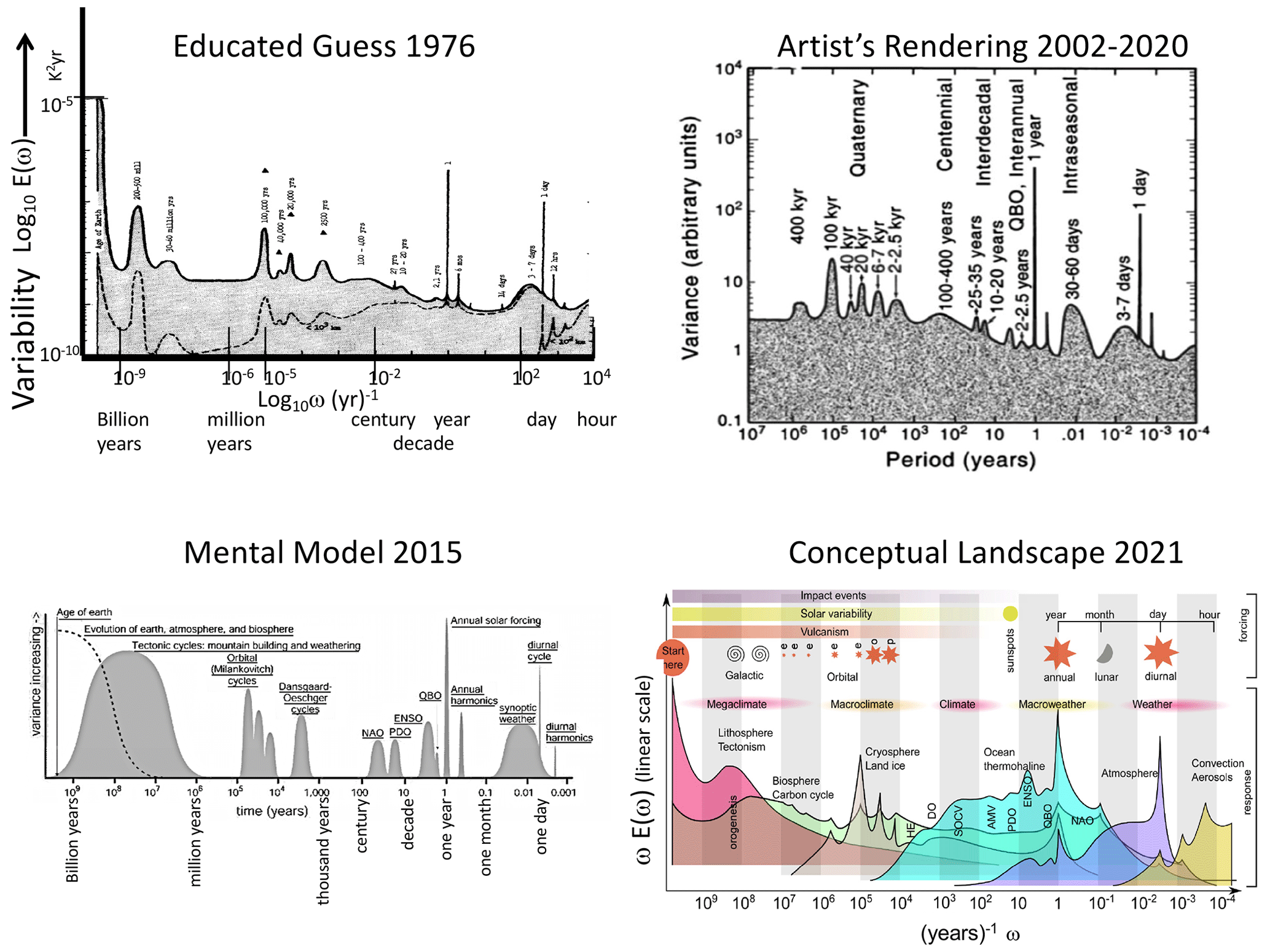
Figure 6The evolution of the scalebound paradigms of atmospheric dynamics (1976–2021). The upper-left “educated guess” is from Mitchell (1976), and the upper-right “artist's rendering” is from Ghil (2002) and Ghil and Lucarini (2020). The lower left shows the NOAA's “mental model” (downloaded from the site in 2015), and the lower right shows the “conceptual model” from von der Heydt et al. (2021).
2.2 The scaling alternative
2.2.1 Scaling as a symmetry
Although scaling in atmospheric science goes back to Richardson in the 1920s, it was the Fractal Geometry of Nature (Mandelbrot, 1977, 1982) that first proposed scaling as a broad alternative to the scalebound paradigm. Alongside deterministic chaos and nonlinear waves, fractals rapidly became part of the nascent nonlinear revolution. In contrast to scaleboundedness, scaling supposes that zooming results in something that is qualitatively unchanged.
Although Mandelbrot emphasized fractal geometry, i.e. the scaling of geometrical sets of points, it soon became clear (Schertzer and Lovejoy, 1985c) that the physical basis of scaling (more generally scaling fields and scaling processes) is in fact a scale-symmetry principle – effectively a scale-conservation law that is respected by many nonlinear dynamical systems, including those governing fluids (Schertzer and Lovejoy, 1985a, 1987; Schertzer et al., 2012).
Scaling is seductive because it is a symmetry. Ever since Noether published her eponymous theorem (Noether, 1918) demonstrating the equivalence between symmetries and conservation laws, physics has been based on symmetry principles. Thanks to Noether's theorem, by formulating scaling as a general symmetry principle, the scaling is the physics. Symmetry principles represent a kind of maximal simplicity, and since “entities must not be multiplied beyond necessity” (Occam's razor), physicists always assume that symmetries hold unless there is evidence for symmetry breaking.
In the case of fluids, we can verify this symmetry on the equations as implemented for example in GCMs (e.g. Stolle et al., 2009, 2012, and the discussion in Sect. 2.2.3) – but only for scales larger than the (millimetric) dissipation scales, where the symmetry is broken and mechanical energy is converted into heat: this is true for Navier–Stokes turbulence; however, the atomic-scale details are not fully clear. Kadau et al. (2010) and Tuck (2008, 2022) argue that scaling can continue to much smaller scales. The scaling is also broken at the large scales by the finite size of the planet. In between, boundary conditions such as the ocean surface or topography might potentially have broken the scaling, but in fact they turn out to be scaling themselves and so do not introduce a characteristic scale (e.g. Gagnon et al., 2006).
In the atmosphere one therefore expects scaling. It is expected to hold unless processes can be identified that act preferentially and strongly enough at specific scales that could break it. This turns the table on scalebound thinking: if we can explain the atmosphere's structure in a scaling manner, then this is the simplest explanation and should a priori be adopted. The onus must be on the scalebound approach to demonstrate the inadequacy of scaling and the need to replace the hypothesis of a unique wide scaling-range regime by (potentially numerous) distinct scalebound mechanisms.
Once a scaling regime is identified – either theoretically or empirically (preferably by a combination of both) – it is associated with a single basic dynamical mechanism that repeats scale after scale over a wide range, and hence it provides an objective classification principle.
2.2.2 Wide-range scaling in atmospheric science
The atmospheric scaling paradigm is almost as old as numerical weather prediction, both being proposed by Richardson in the 1920s. Indeed, ever since Richardson's scaling law of turbulent diffusion (Richardson, 1926 – the precursor of the better-known Kolmogorov law, Kolmogorov, 1941), scaling has been the central turbulence paradigm.
From the beginning, Richardson argued for a wide-range scaling holding from millimetres to thousands of kilometres (Fig. 7). Richardson himself attempted an empirical verification, notably using data from pilot balloons and volcanic ash (and later – in the turbulent ocean – with bags of parsnips that he watched diffusing from a pier on Loch Lomond; Richardson and Stommel, 1948). However, there remained a dearth of data spanning the key “mesoscale” range ≈ 1–100 km corresponding to the atmosphere's scale height, so that for several decades following Richardson, progress in atmospheric turbulence was largely theoretical. In particular, in the 1930s the turbulence community made rapid advances in understanding the simplified isotropic turbulence problem, notably the Karman–Howarth equations (Karman and Howarth, 1938) and the discovery of numerous isotropic scaling laws for passive scalar advection and for mechanically driven and buoyancy-driven turbulence. At first, Kolmogorov and the other pioneers recognized that atmospheric stratification strongly limited the range of applicability of isotropic laws. Kolmogorov, for example, estimated that his famous law of 3D isotropic turbulence would only hold at scales below 100 m. As discussed in Sect. 4, modern data show that this was a vast overestimate: if his isotropic law ever holds anywhere in the atmosphere, it is below 5 m. However, at the same time, in the horizontal, the anisotropic generalization of the Kolmogorov law apparently holds up to planetary scales.
In the 1970s, motivated by Charney's isotropic 2D geostrophic turbulence (Charney, 1971), the ambitious “EOLE” experiment was undertaken specifically to study large-scale atmospheric turbulence. EOLE (for the Greek wind god) ambitiously used a satellite to track the diffusion of hundreds of constant-density balloons (Morel and Larchevêque, 1974), but the results turned out to be difficult to interpret. Worse, the initial conclusions – that the mesoscale wind did not follow the Kolmogorov law – turned out to be wrong, and they were later re-interpreted (Lacorta et al., 2004) and then further re-re-interpreted (Lovejoy and Schertzer, 2013), finally vindicating Richardson nearly 90 years later.
Therefore, when Lovejoy (1982), benefitting from modern radar and satellite data, discovered scaling right through the mesoscale (Fig. 7, right), it was the most convincing support to date for Richardson's daring 1926 wide-range scaling hypothesis. Although at first it was mostly cited for its empirical verification that clouds were indeed fractals, today, 40 years later, we increasingly appreciate its vindication of Richardson's scaling from 1 to 1000 km, right through the mesoscale. It marks the beginning of modern scaling theories of the atmosphere. This has since been confirmed by massive quantities of remotely sensed and in situ data, both on Earth (Fig. 8) and more recently on Mars (Fig. 9, discussed in detail in Sect. 3.4).
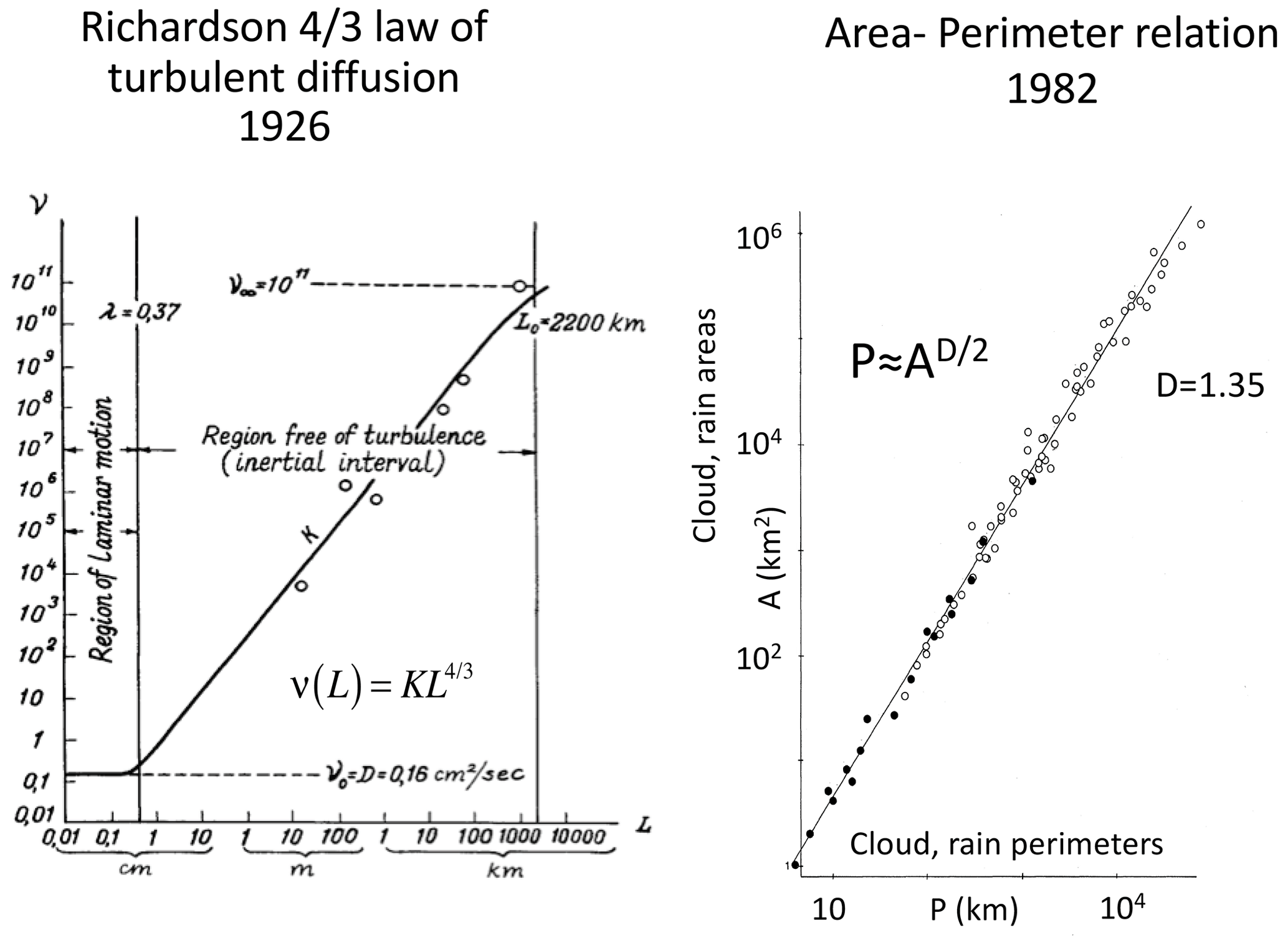
Figure 7Richardson's pioneering scaling model (Richardson, 1926) of turbulent diffusion (left) with an early update (Lovejoy, 1982) (right) using radar rain data (black) and satellite cloud data (open circles).
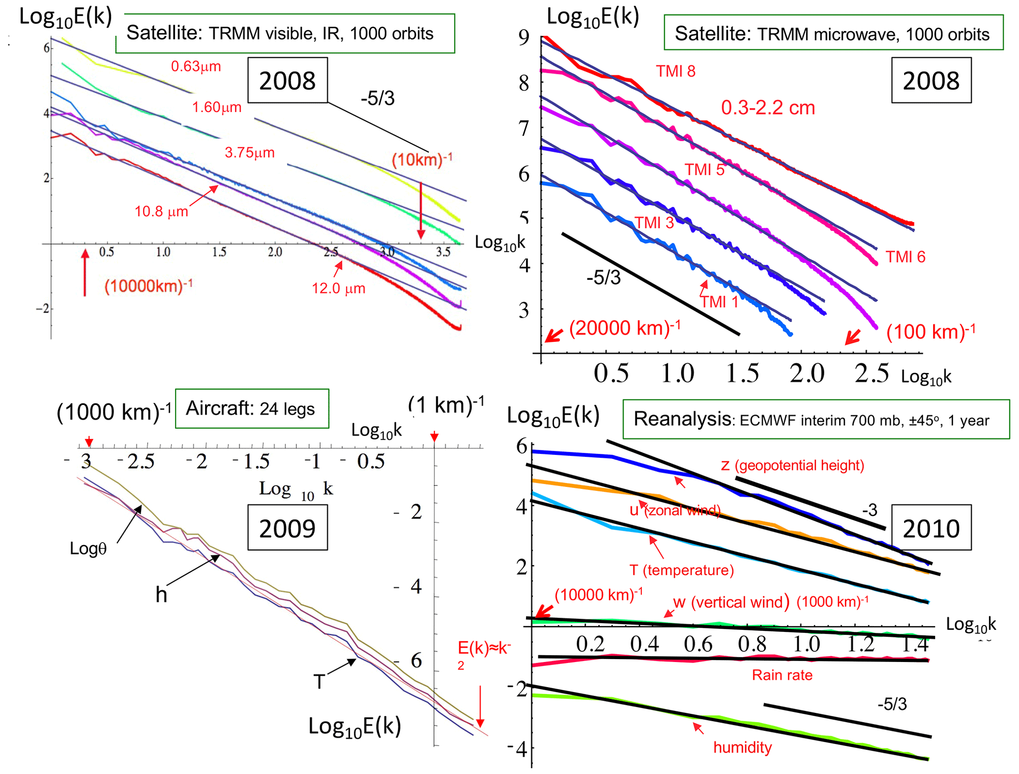
Figure 8Planetary-scale power-law spectra () from satellite radiances (top), aircraft (bottom left), and reanalyses (bottom right). Upper right: spectra from over 1000 orbits of the Tropical Rainfall Measurement Mission (TRMM), of five channels visible through thermal IR wavelengths displaying the very accurate scaling down to scales of the order of the sensor resolution (≈ 10 km). Adapted from Lovejoy et al. (2008b). Upper left: spectra from five other (microwave) channels from the same satellite. The data are at lower resolution, and the latter depend on the wavelength: again, the scaling is accurate up to the resolution. Adapted from Lovejoy et al. (2008b). Lower left: the spectrum of temperature (T), humidity (h), and log potential temperature (logθ) averaged over 24 legs of aircraft flight over the Pacific Ocean at 200 mb. Each leg had a resolution of 280 m and had 4000 points (1120 km). A reference line corresponding to the k−2 spectrum is shown in red. The mesoscale (1–100 km) is right in the middle of the figure and is not at all visible. Adapted from Lovejoy et al. (2010). Lower right: zonal spectra of reanalyses from the European Centre for Medium-Range Weather Forecasts (ECMWF), once daily for the year 2008 over the band ±45∘ latitude. Adapted from Lovejoy and Schertzer (2011).
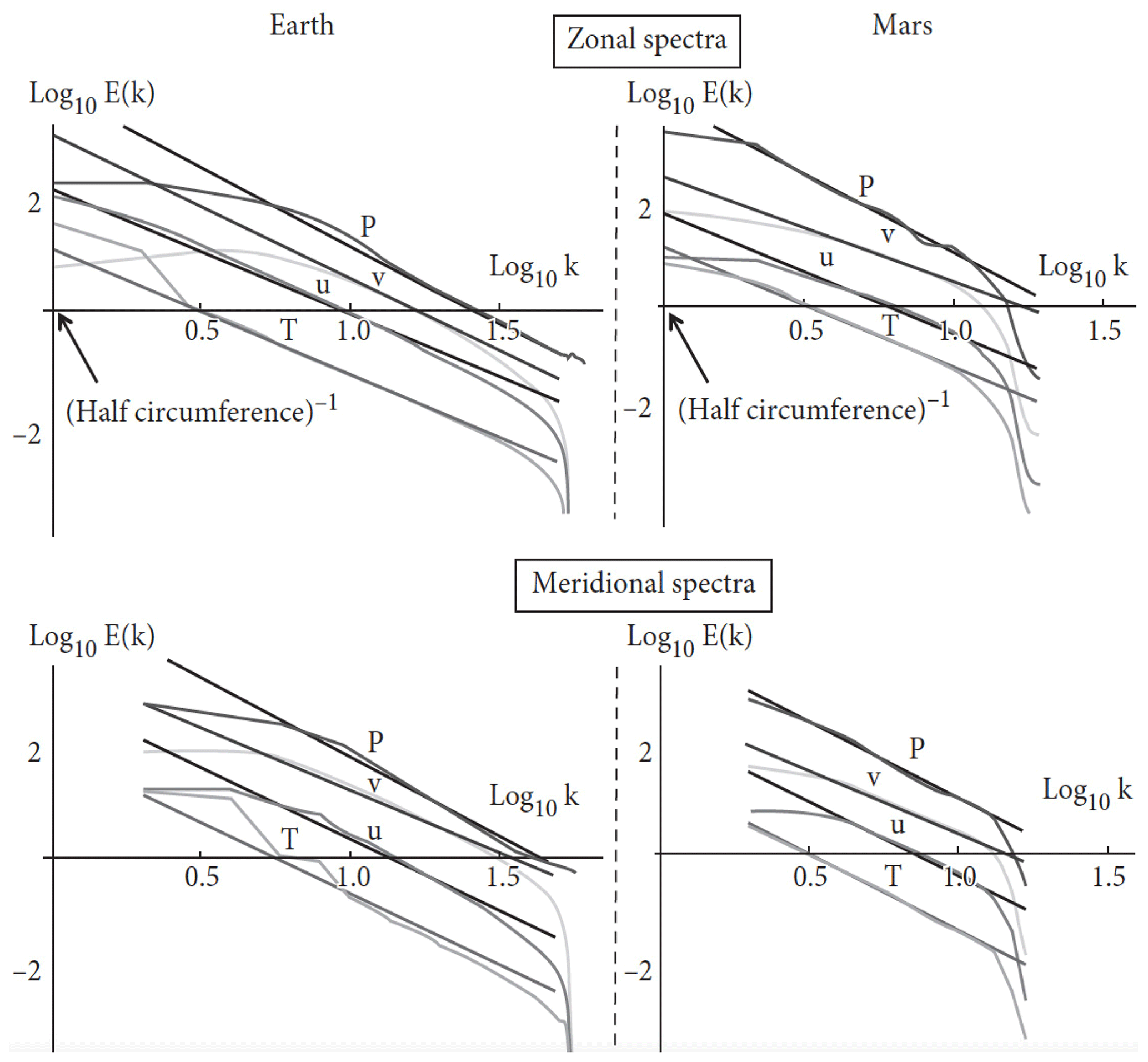
Figure 9Earth (left) and Mars (right). The zonal spectra (top right) of Mars as functions of the nondimensional wavenumbers for pressure (p, purple), meridional wind (v, green), the zonal wind (u, blue), and temperature (T, red). The data for Earth were taken for the year 2006 at 69 % atmospheric pressure between latitudes ±45∘. The data for Mars were taken at 83 % atmospheric pressure for Martian years 24 to 26 between latitudes ±45∘. The reference lines (in all the plots) have absolute slopes from top to bottom: β=3.00, 2.05, 2.35, and 2.35 (for , and T respectively). The spectra have been rescaled and an offset added for clarity. Wavenumber k=1 corresponds to the half-circumference of the respective planets. Reproduced from Chen et al. (2016).
2.2.3 Which is more fundamental: scaling or isotropy?
In Sect. 2.1, we discussed the debate between scaling and mechanistic, generally deterministic, scalebound approaches. However, even in the statistical (turbulence) strand of atmospheric science, there evolved an alternative to Richardson's wide-range scaling: the paradigm of isotropic turbulence.
In the absence of gravity (or another strong source of anisotropy), the basic isotropic scaling property of the fluid equations has been known for a long time (Taylor, 1935; Karman and Howarth, 1938). The scaling symmetry justifies the numerous classical fluid dynamics similarity laws (e.g. Sedov, 1959), and it underpins models of statistically isotropic turbulence, notably the classical turbulence laws of Kolmogorov (Kolmogorov, 1941), Bolgiano and Obukhov (buoyancy-driven, Sect. 4.1) (Bolgiano, 1959; Obukhov, 1959), and Corrsin and Obukhov (passive scalar) (Corrsin, 1951; Obukhov, 1949).
These classical turbulence laws can be expressed in the form
where scale was interpreted in an isotropic sense, H is the fluctuation exponent, and, physically, the turbulent fluxes are the drivers (compare with Eq. 2). The first and most famous example is the Kolmogorov law for fluctuations in the wind, where the turbulent flux is the energy rate density (ε, ) and . Equation (4) is the same as Eq. (2), except that the randomness is hidden in the turbulent flux that classically was considered to be quasi-Gaussian, the non-intermittent special case (Sect. 3.2).
Theories and models of isotropic turbulence were developed to understand the fundamental properties of high Reynolds number turbulence, and this was independent of whether or not it could be applied to the atmosphere. Since the atmosphere is a convenient very high Reynolds number laboratory (Re≈1012), the question is therefore “Is isotropic turbulence relevant in the atmosphere?” (the title of Lovejoy et al., 2007).
Figure 10 graphically shows the problem: although the laws of isotropic turbulence are themselves scaling, they imply a break in the middle of the “mesoscale” at around 10 km. To model the larger scales, Fjortoft (1953) and Kraichnan (1967) soon found another isotropic scaling paradigm: 2D isotropic turbulence. Charney in particular adapted Kraichnan's 2D isotropic turbulence to geostrophic turbulence (Charney, 1971), and the result is sometimes called “layerwise” 2D isotropic turbulence. While Kraichnan's 2D model was rigidly flat with strictly no vortex stretching, Charney's extension allowed for some limited vortex stretching. Figure 10 shows the implied difference between the 2D isotropic and 3D isotropic regimes.
Even though isotropy had originally been proposed purely for theoretical convenience, armed with two different isotropic scaling laws, it was now being proposed as the fundamental atmospheric paradigm. If scaling in atmospheric turbulence is always isotropic, then we are forced to accept a scale break. The assumption that isotropy is the primary symmetry implies (at least) two scaling regimes with a break (presumably) near the 10 km scale height, i.e. in the mesoscale. The 2D–3D model with its implied “dimensional transition” (Schertzer and Lovejoy, 1985c) already contradicted the wide-range scaling proposed by Richardson.
An important point is that the implied scale break is neither physically nor empirically motivated: it is purely a theoretical consequence of assuming the predominance of isotropy over scaling. One is forced to choose: which of the fundamental symmetries is primary, isotropy or scaling?
By the time a decade later that the alternative (wide-range) anisotropic scaling paradigm (see Fig. 11 for a schematic) was proposed (Schertzer and Lovejoy, 1985c, a), Charney's beautiful theory along with its 2D–3D scale break had already been widely accepted, and even today it is still taught. More recently (Schertzer et al., 2012), generalized scale invariance was linked directly to the governing equations, so that a clear anisotropic theoretical alternative to Charney's isotropic theory is available.
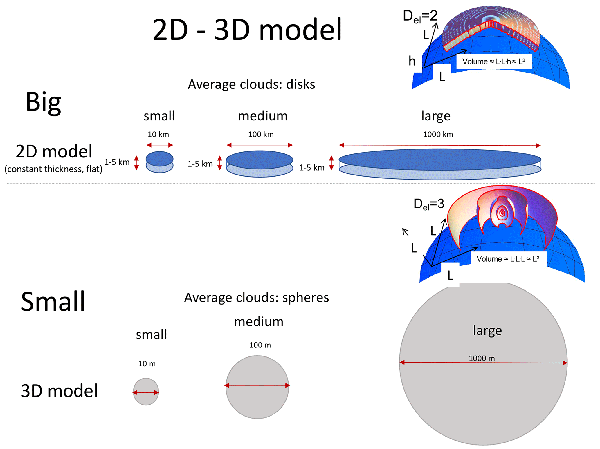
Figure 10A schematic showing the geometry of isotropic 2D models (top, for the large scales); the volumes of average structures (disks) increase as the square of the disk diameter. The isotropic 3D model is a schematic of 3D turbulence models for the small scales, with the volumes of the spheres increasing as the cube of the diameter. These geometries are superposed on the Earth's curved surface (the blue spherical segments on the right). We see (bottom right, Earth's surface) that – unless they are strongly restricted in range – the 3D isotropic models quickly imply structures that extend into outer space.
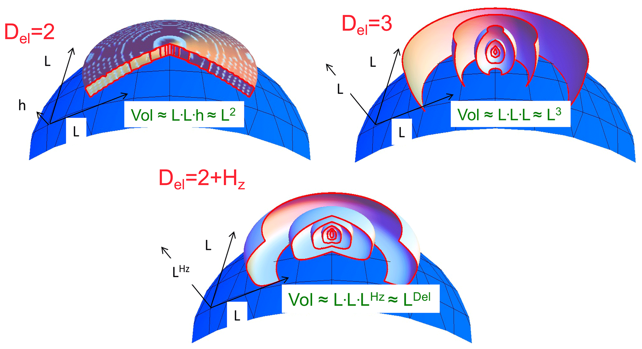
Figure 11A schematic diagram showing the change in shape of average structures which are isotropic in the horizontal (slightly curved to indicate the Earth's surface) but with scaling stratification in the vertical. Hz increases from 0 (upper left) to 1 (lower right) with an effective “elliptical dimension” . In order to illustrate the change in structures with scale, the ratio of tropospheric thickness to Earth's radius has been increased by nearly a factor of 1000. Note that, in the Del=3 case, the cross sections are exactly circles; the small distortion is an effect of perspective due to the mapping of the structures onto the curved surface of the Earth. Reproduced from Lovejoy and Schertzer (2010c).
2.3 Aspects of scaling in one dimension
The basic signature of scaling is a power-law relation of a statistical characteristic of a system as a function of space scale and/or timescale. In the empirical test of the Richardson law (Fig. 7, left panel), it is the turbulent viscosity as a function of horizontal scale that is a power law. On the right-hand side, it is rather the complicated (fractal) perimeters of clouds and rain zones that are power-law functions of the corresponding areas. The Fig. 7 analysis methods lack generality, so let us instead consider spectra (Fourier space) and, then, fluctuations (real space, Sect. 2.5, Appendix B).
Following Mitchell, we may consider variability in the spectral domain: for example, the power spectrum of the temperature T(t) is
where is its Fourier transform and ω is the frequency. A scaling process E(ω) has the same form if we consider it at a timescale λ times smaller or, equivalently, at a frequency λ times larger:
where β is the “spectral exponent”. The solution of this functional equation is a power law:
Therefore, a log–log plot of the spectrum as a function of frequency will be a straight line; see Fig. 12 for early quantitative applications to climate series.
Alternatively, we can consider scaling in real space. Due to “Tauberian theorems” (e.g. Feller, 1971), power laws in real space are transformed into power laws in Fourier space (and vice versa). This result holds whenever the scaling range is wide enough – i.e. even if there are high- and/or low-frequency cutoffs (needed if only for the convergence of the transforms). If we consider fluctuations ΔT over time interval Δt, then if the system is scaling, we can introduce the (“generalized”, qth-order) structure function as
where the “〈〉” sign indicates statistical (ensemble) averaging (assuming statistical stationarity, there is no t dependence). Once again, classical fluctuations are defined simply as differences, i.e. , although more general fluctuations are needed as discussed in Sect. 2.5. For stationary scaling processes, the Wiener–Khintchin theorem implies a simple relation between real space and Fourier scaling exponents:
(the “2” is because the variance is a second-order moment). If, in addition, the system is “quasi-Gaussian”, then S2 gives a full statistical characterization of the process. Therefore, often only the second-order structure function S2(Δt) is considered (e.g. Fig. 12, top). However, as discussed above, geo-processes are typically strongly intermittent and rarely quasi-Gaussian, and the full exponent function ξ(q) is needed (Sect. 3.1). In the next section, we discuss this figure in more detail, including its physical implications. For the moment, simply note the various linear (scaling) regimes in the log–log plots.
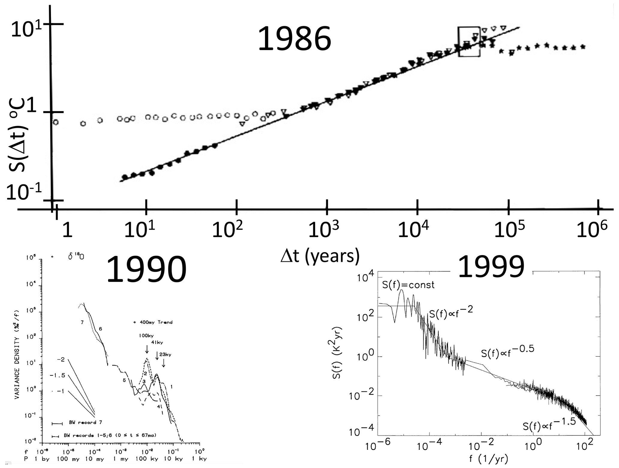
Figure 12The evolution of the scaling picture for 1986–1999. Top: the rms difference structure functions estimated from local (central England) temperatures since 1659 (open circles, upper left), Northern Hemisphere temperature (black circles), and paleotemperatures from Vostok (Antarctic, solid triangles), Camp Century (Greenland, open triangles), and an ocean core (asterisks). For the Northern Hemisphere temperatures, the (power-law, linear in this plot) climate regime starts at about 10 years. The reference line has a slope H=0.4. The rectangle (upper right) is the “glacial–interglacial window” through which the structure function must pass in order to account for typical variations of ±2 to ±3 K for cycles with half-periods ≈ 50 kyr. Reproduced from Lovejoy and Schertzer (1986b). Note the two essentially flat sets of points, one from the local central England temperature up to roughly 300 years and the other from an ocean core that is flat from scales 100 000 years and longer. These correspond to the macroweather and macroclimate regimes where H<0, so that the flatness is an artefact of the use of differences in the definition of fluctuations (Appendix B2). Bottom left: composite spectrum of δ18O paleotemperatures from Shackleton and Imbrie (1990). Bottom right: composite using instrumental temperatures (right) and paleotemperatures (left) with piecewise linear (power-law) reference lines. The composite is not very different from the updated one shown in Fig. 13. The lower-right composite is reproduced from Pelletier (1998).
2.4 The impact of data on the scalebound view
In spite of its growing disconnect with modern data, Mitchell's figure and its scalebound updates continue to be influential. However, within 15 years of Mitchell's famous paper, two scaling composites, over the ranges 1 h to 105 years and 103 to 108 years, already showed huge discrepancies (Lovejoy and Schertzer, 1986b; Fig. 12, top panel; Shackleton and Imbrie, 1990, bottom left; see also Pelletier, 1998, bottom right, and Huybers and Curry, 2006). Returning to Mitchell's original figure, Lovejoy (2015) superposed the spectra of several modern instrumental and paleo series; the differences are literally astronomical (Fig. 13). While over the range 1 h to 109 years, Mitchell's background varies by a factor ≈ 150, the spectra from real data imply that the true range is a factor greater than a quadrillion (1015).
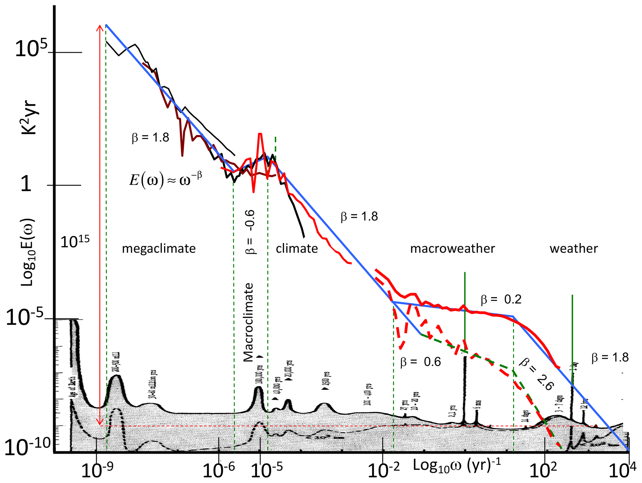
Figure 13A comparison of Mitchell's educated guess of a log–log spectral plot (grey, bottom, Mitchell, 1976) superposed with modern evidence from spectra of a selection of the series described in Table 1 and Lovejoy (2015) from which this figure is reproduced. On the far right, the spectra from the 1871–2008 20CR (at daily resolution) quantify the difference between the globally averaged temperature (bottom right, red line) and local averages (2∘ × 2∘, top right, red line). The spectra were averaged over frequency intervals (10 per factor of 10 in frequency), thus “smearing out” the daily and annual spectral “spikes”. These spikes have been re-introduced without this averaging and are indicated by green spikes above the red daily-resolution curves. Using the daily-resolution data, the annual cycle is a factor ≈ 1000 above the continuum, whereas using hourly-resolution data, the daily spike is a factor ≈ 3000 above the background. Also shown is the other striking narrow spectral spike at (41 kyr)−1 (obliquity circa a factor of 10 above the continuum); this is shown in dashed green since it is only apparent over the period 0.8–2.56 Myr BP (before present). The blue lines have slopes indicating the scaling behaviours. The thin dashed green lines show the transition periods that separate out the scaling regimes; these are (roughly) at 20 d, 50 years, 80 000 years, and 500 000 years. This is reproduced from Lovejoy (2015).
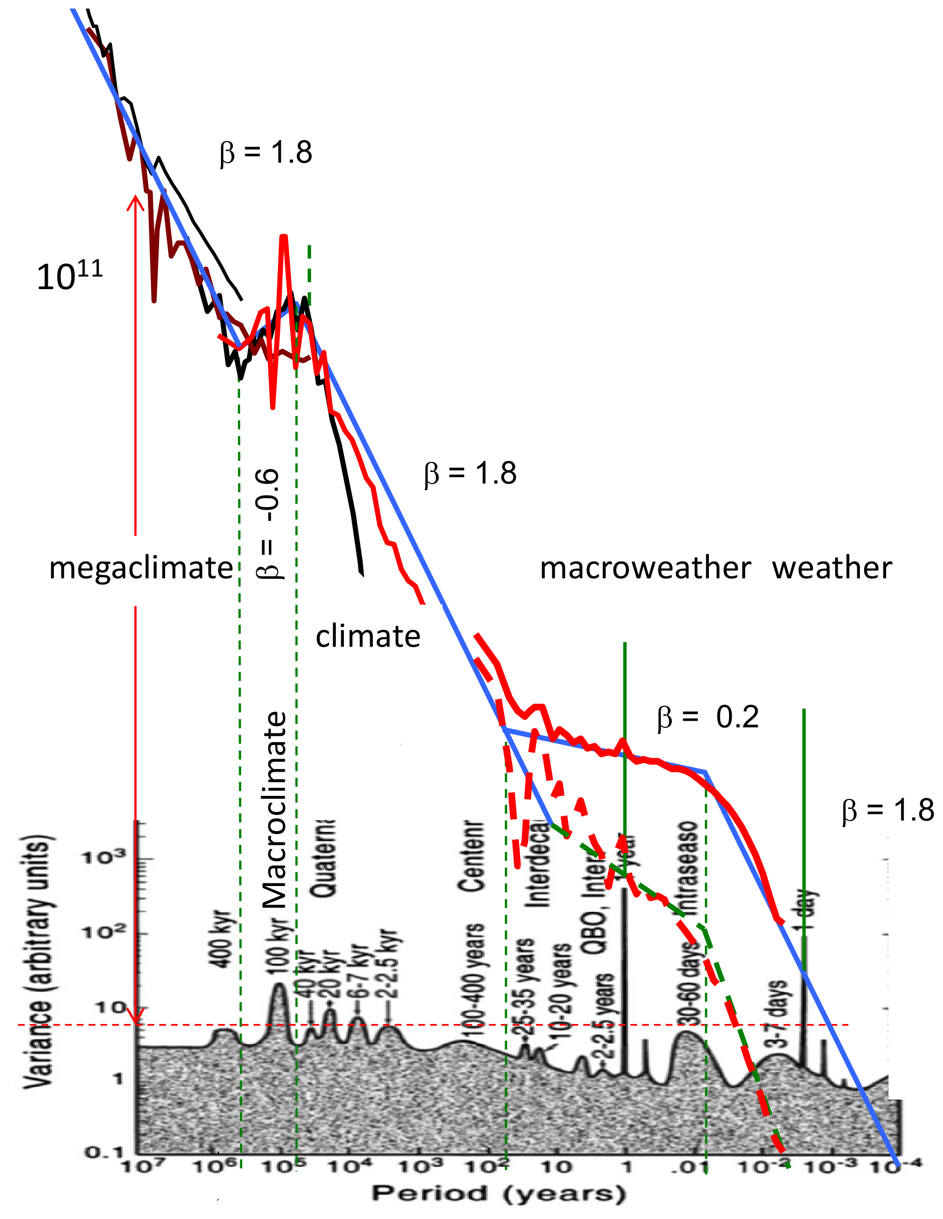
Figure 14Artist's rendering with data superposed. Adapted from Ghil (2002) and reprinted in Ghil and Lucarini (2020).
Returning to the artist's rendering, Fig. 14 shows that, when compared to the data, it fares no better than Mitchell's educated guess. The next update – the NOAA's mental model – only specified that its vertical axis be proportional to “variability”. If we interpret variability as the root-mean-square (rms) fluctuation at a given scale and the flat “background” between the bumps as white noise, then we obtain the comparison in Fig. 15. Although the exact definition of these fluctuations is discussed in Sect. 2.5, they give a directly physically meaningful quantification of the variability at a given timescale. In Fig. 15, we see that the mental model predicts that successive average Earth temperatures of 1 million years would differ by only tens of micro-Kelvin. A closely similar conclusion would hold if we converted Mitchell's spectrum into rms real-space fluctuations.
The most recent scalebound update – the “conceptual landscape” – is compared with modern data in Fig. 16. Although the various scaling regimes proposed in Lovejoy (2013) (updated in Fig. 18 and discussed below) are discreetly indicated in the background, in many instances, there is no obvious relation between the regimes and the landscape. In particular, the word “macroweather” appears without any obvious connection to the figure, but even the landscape's highlighted scalebound features are not very close to the empirical curve (red). Although the vertical axis is only “relative”, this quantitative empirical comparison was made by exploiting the equal-area property mentioned above. The overlaid solid red curve was estimated by converting the disjoint spectral power laws shown in the updated Mitchell graph (Fig. 8). In addition, there is also an attempt to indicate the amplitudes of the narrow spectral spikes (the green spikes in Fig. 13) at diurnal, annual, and – for the epoch 2.5–0.8 Myr – obliquity spectral peaks at (41 kyr)−1. In conclusion, the conceptual landscape bears little relation to the real world.
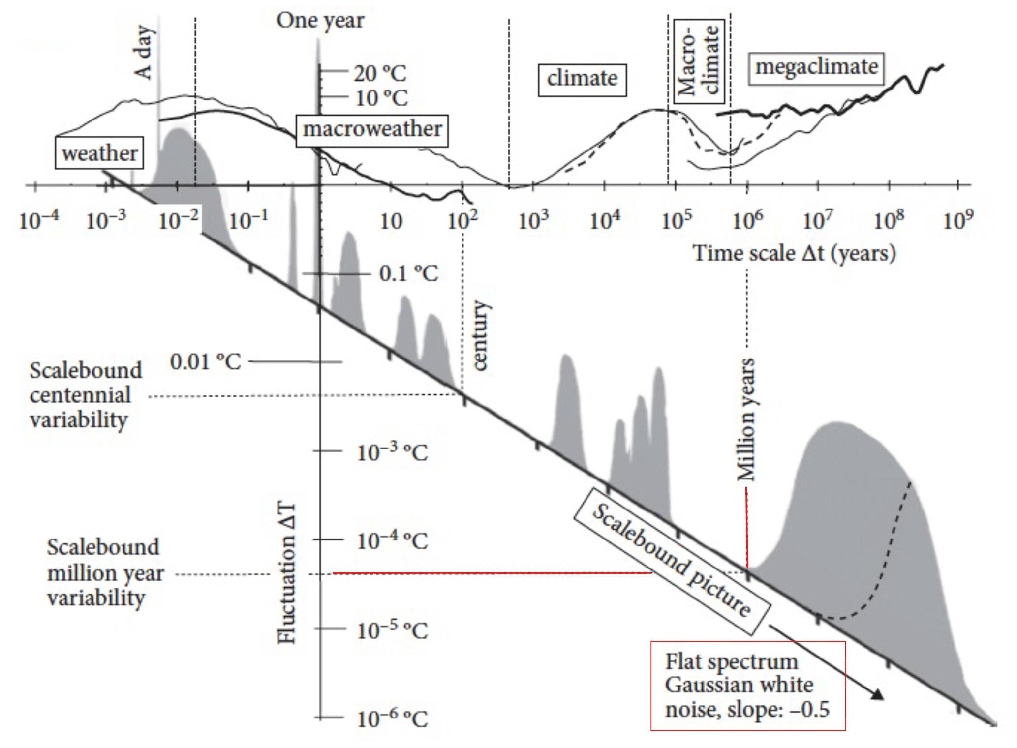
Figure 15Mental model with data. The data spectrum in Fig. 13 is replotted in terms of fluctuations (grey, top; see Fig. 17). The diagonal axis corresponds to the flat baseline of Fig. 6 (lower left) that now has a slope of corresponding to an uncorrelated Gaussian “white noise” background. Since the amplitudes in Fig. 6 (lower left) were not specified, the amplitudes of the transformed “bumps” are only notional. At the top are superposed the typical Haar fluctuations at timescale Δt as estimated from various instrumental and paleo-series, from Fig. 17 (bottom, using the data displayed in Fig. 2). We see (lower right) that consecutive 1 Myr averages would only differ by several micro-Kelvin. Reproduced from Lovejoy (2019).
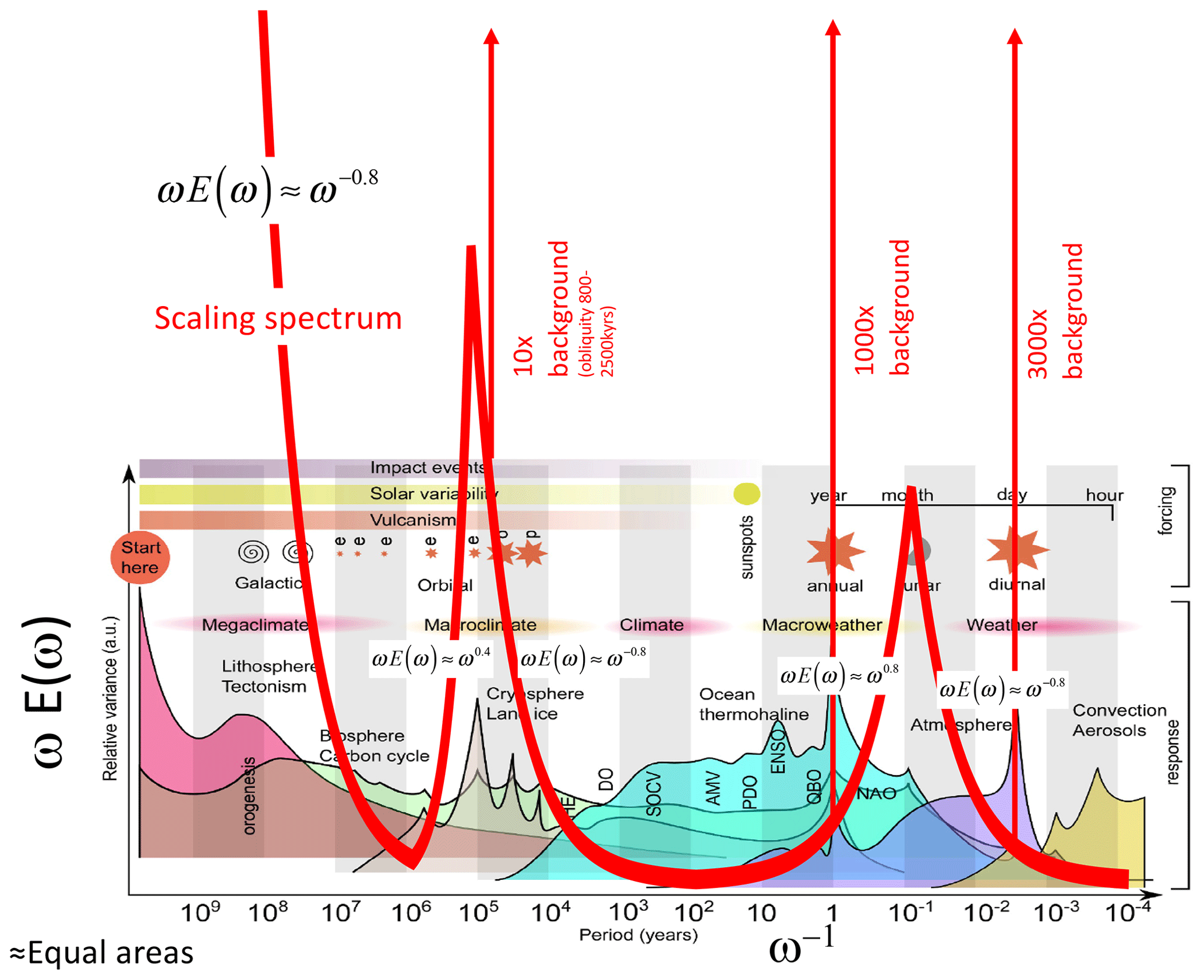
Figure 16Conceptual landscape with data. The superposed red curves use the empirical spectra in Fig. 13 and adjust the (linear) vertical scale for a rough match with the landscape. The vertical lines indicate huge periodic signals (the diurnal and annual cycles on the right and on the left, the obliquity signal seen in spectra between 0.8 and 2.5 Myr ago). Adapted from von der Heydt et al. (2021).
2.5 Revisiting the atmosphere with the help of fluctuation analysis
The scalebound framework for atmospheric dynamics emphasized the importance of numerous processes occurring at well-defined timescales, the quasi-periodic “foreground” processes illustrated as bumps – the signals – on Mitchell's nearly flat background. The point here is not that these processes and mechanisms are wrong or non-existent: it is rather that they only explain a small fraction of the overall variability, and this implies that they cannot be understood without putting them in the context of their dynamical (scaling) regime. This was also demonstrated quantitatively and explicitly over at least a significant part of the climate range by Wunsch (2003).
One of the lessons to be drawn from the educated guesses, artists' renderings, and conceptual landscapes is that, although spectra can be calculated for any signal, the interpretations are often not obvious. The problem is that we have no intuition about the physical meaning of the units – K2 s, K2 yr, or even K2 Myr – so that often (as here) the units used in spectral plots are not even given. It then becomes impossible to take data from disparate sources and at different timescales to make the spectral composites needed to make a meaningful check of the scalebound paradigm.
The advantage of fluctuations such as in Fig. 12 (top) is that the numbers – e.g. the rms temperature fluctuations at some scale – have a straightforward physical interpretation. However, the differences used to define fluctuations (see Fig. 17, top) have a non-obvious problem: on average, differences cannot decrease with increasing time intervals (in Appendix B, this problem is discussed more precisely in the Fourier domain). This is true for any series that has correlations that decrease with Δt (as physically relevant series always do). A consequence is that whenever the value of ξ(2) is negative – implying that the mean fluctuations decrease with scale – the difference fluctuations will at best give a constant result (the flat parts of Fig. 12, top).
However, do regions of negative ξ(2) exist? One way to investigate this is to try to infer the exponent ξ(2) from the spectrum that does not suffer from an analogous restriction: its exponent β can take any value. In this case we can use the formula (Eq. 9). The latter implies that negative ξ(2) corresponds to β<1, and a check on the spectrum in Fig. 7 indicates that several regions (notably the macroweather regime) are indeed flat enough (β<1) to imply negative ξ(2). How do we fix the problem and estimate the correct ξ(2) when it is negative?
It took a surprisingly long time to clarify this issue. To start with, in classical turbulence, ξ(2)>0 (e.g. the Kolmogorov law), there was no motivation to look further than differences. Mathematically, the main advance came in the 1980s from wavelets. It turns out that, technically, fluctuations defined as differences are indeed wavelets, but mathematicians mock them, calling them the poor man's wavelet, and they generally promote more sophisticated wavelets (see Appendix B2): the simplicity of the physical interpretation is not their concern. This was the situation in the 1990s, when scaling started to be systematically applied to geophysical time series involving negative ξ(2) (i.e. to any macroweather series, although at the time this was not clear). A practical solution adopted by many was to use the detrended fluctuation analysis (DFA) method (Peng et al., 1994). One reason the DFA method is popular is that the raw DFA fluctuations are not too noisy. However, this is in fact an artefact since they are fluctuations of the running sum of the process, not of the process itself. When DFA fluctuations of the process are used, they are just as variable as the Haar fluctuations (Lovejoy and Schertzer, 2012a; Hébert et al., 2021a). Unfortunately, DFA fluctuations are difficult to interpret, so that typically only exponents are extracted: the important information contained in the fluctuation amplitudes is not exploited (see Appendix B).
New clarity was achieved with the help of the (first) Haar wavelet (Haar, 1910). There were two reasons for this: the simplicity of its definition and calculation and the simplicity of its interpretation (Lovejoy and Schertzer, 2012a). To determine the Haar fluctuation over a time interval Δt, one simply takes the average of the first half of the interval and, from this, subtracts the average of the second half (Fig. 17, bottom; see Appendix B2 for more details). As for the interpretation, when H is positive, then it is (nearly) the same as a difference, whereas whenever H is negative, the fluctuation can be interpreted as an “anomaly” (in this context, an anomaly is simply the average over a segment length Δt of the series with its long-term average removed, Appendix B2). In both cases we also recover the correct value of the exponent H. Although the Haar fluctuation is only useful for H in the range −1 to 1, this turns out to cover most of the series that are encountered in geoscience.
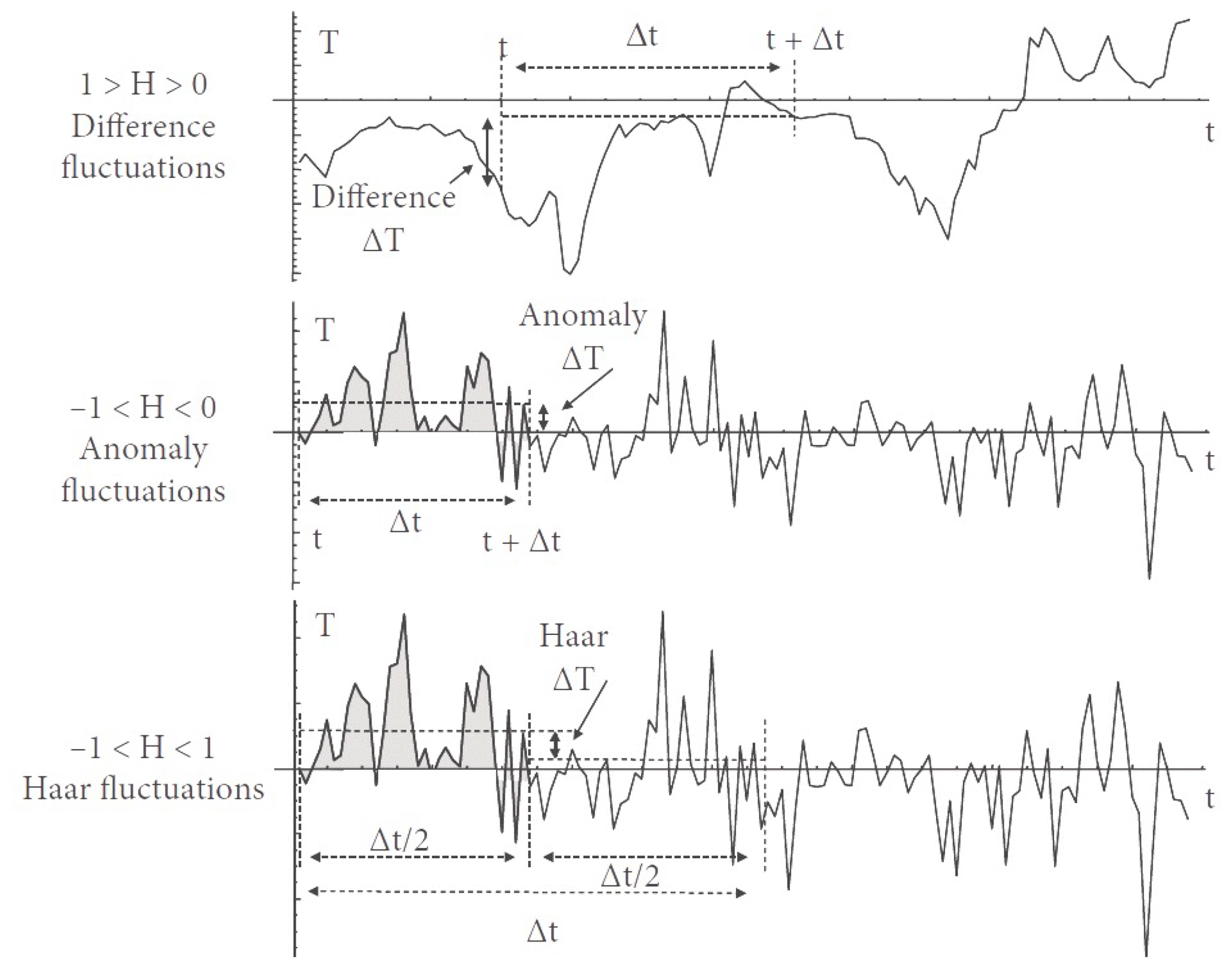
Figure 17Schematic illustration of difference (top) and anomaly (middle) fluctuations for a multifractal simulation of the atmosphere in the weather regime (), top, and in the lower-frequency macroweather regime (), middle. Note the wandering or drifting of the signal in the top panel and the cancelling behaviour in the middle one. The bottom panel is a schematic illustration of Haar fluctuations (useful for processes with ). The Haar fluctuation over the interval Δt is the mean of the first half subtracted from the mean of the second half of the interval Δt. Reproduced from Lovejoy (2019).
Figure 18 shows a modern composite using the rms Haar fluctuation, spanning a range of scales of ≈ 1017 (compare this with Fig. 12, top, for the earlier version using fluctuations as differences). The same five regimes as in Fig. 13 are shown, but now the typical variations in temperature over various timescales are very clear.
Also shown in Fig. 16 are reference lines indicating the typical scale dependencies. These correspond to typical temperature fluctuations , where ξ(1)=H is the “fluctuation exponent” (the exponent of the mean absolute fluctuation, the relationship ξ(2)=2H, is valid if we ignore intermittency: it is the quasi-Gaussian relationship still often invoked; see Eq. 15). In the figure, we see that the character of the regimes alternates between regimes that grow (H>0) and ones that decrease (H<0) with timescale. The sign of H has a fundamental significance; to see this, we can return to typical series over the various regimes in Fig. 2 (left-hand-side column). In terms of their visual appearances, the H>0 regimes have signals that seem to “wander” or “drift”, whereas for H<0 regimes, fluctuations tend to cancel. In the former, waiting longer and longer typically leads to larger changes in temperature, whereas in the latter, longer and longer temporal scales lead to convergence to well-defined values.
With the help of the figure, we can now understand the problem with the usual definition of climate as “long-term” weather. As we average from 10 d to longer durations, temperature fluctuations do indeed tend to diminish – as expected if they converged to the climate. Consider for example the thick solid line in Fig. 18 (corresponding to data at 75∘ N), which shows that, at about 10 d, the temperature fluctuations are 3 K ( K), diminishing at 20 years to .3 K. Since H<0, the Haar fluctuations are nearly equivalent to the anomalies, i.e. to averages of the series with the long-time mean removed. Over this range, increasing the scale leads to smaller and smaller fluctuations about the point of the apparent point of convergence: the average climate temperature. Figure 18 also shows the longer scales deduced purely from paleodata (isotope ratios from either ice or ocean cores).
The interpretation of the apparent point of convergence as the climate state is supported by the analysis of global data compared with GCMs in “control runs” (i.e. with fixed external conditions, Fig. 19). When averaged over long enough times, the control runs do indeed converge, although the convergence is “ultra slow” (at a rate characterized by the exponent 0.15 for the GCMs). Extrapolating from the figure shows that, even after averaging over 1 million simulated years, the GCMs would still typically be only within ±0.01 K of their respective climates.
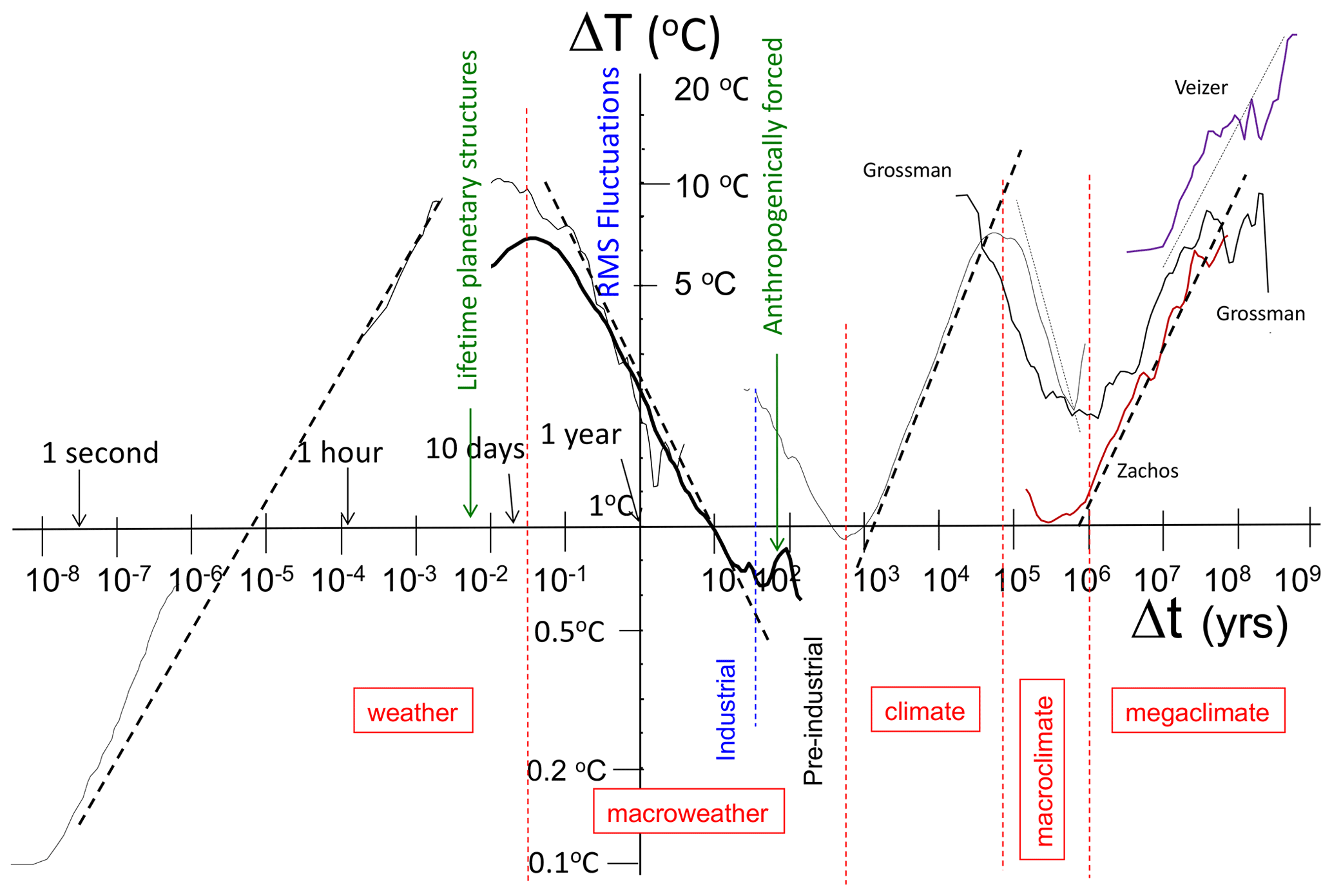
Figure 18The broad sweep of atmospheric variability with rms Haar fluctuations showing the various (roughly power-law) atmospheric regimes, adapted and updated from the original (Lovejoy, 2013) and the update in Lovejoy (2015), where the full details of the data sources are given (with the exception of the paleo-analysis marked “Grossman”, which is from Grossman and Joachimski, 2022). The dashed vertical lines show the rough divisions between regimes; the macroweather–climate transition is different in the preindustrial epoch. Starting at the left, we have, the high-frequency analysis (lower left) from thermistor data taken at McGill at 15 Hz. Then, the thin curve starting at 2 h is from a weather station, the next (thick) curve is from the 20th century reanalysis (20CR), and the next, “S”-shaped curve is from the EPICA core. Finally, the three far-right curves are benthic paleotemperatures (from “stacks”). The quadrillion estimate is for the spectrum: it depends somewhat on the calibration of the stacks. With the calibration in the figure, the typical variation of consecutive 50 million year averages is ±4.5 K (Δt=108 years, rms ΔT=9 K). If the calibration is lowered by a factor of ≈ 3 (to variations of ±1.5 K), then the spectrum would be reduced by a factor of 9. On the other hand, the addition of the 0.017 s resolution thermistor data increases the overall spectral range by another factor of 108 for a total spectral range of a factor ≈ 1017 for scales from 0.017 s to 5 × 10⁸ years.
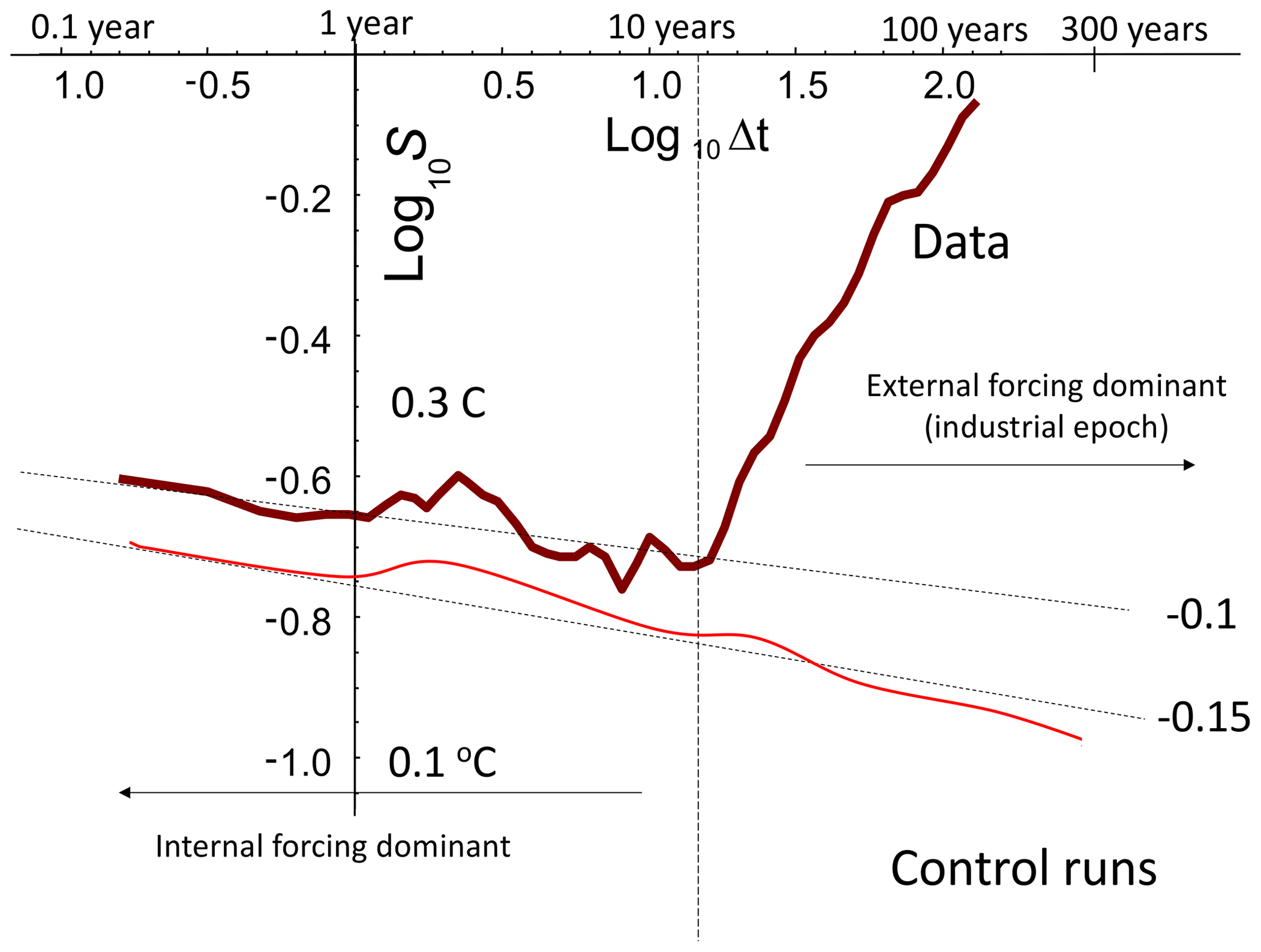
Figure 19Top (brown): the globally averaged, rms Haar temperature fluctuations averaged over three data sets (adapted from Lovejoy, 2019, where there are full details: the curve over the corresponding timescale range in Fig. 19 is at 75∘ N and is a bit different). At small timescales, one can see reasonable power-law behaviour with .1. However, for scales longer than about 15 years, the externally forced variability becomes dominant, although, in reality, the internal variability continues to larger scales and the externally forced variability to smaller ones. The two can roughly be separated at decadal scales as indicated by the vertical dashed line. The curve is reproduced from Lovejoy (2017a). Bottom (red): the rms Haar fluctuations for 11 control runs from the Climate Model Intercomparison Project 5 (CMIP5). The reference slope .15 is adapted from Lovejoy (2019).
Returning to Fig. 18, however, we see that, beyond a critical timescale τc, the convergence is reversed and fluctuations tend rather to increase with timescale. In the Anthropocene (roughly since 1900), the ≈ 15-year timescale where fluctuations stop decreasing and begin increasing with scale is roughly the time that it has taken for anthropogenic warming (over the last decades) to become comparable to the natural internal variability (about ±0.2 K for these globally averaged temperatures). However, for the preindustrial epoch (see the “S”-shaped paleotemperature curve from the EPICA (European Project for Ice Coring in Antarctica) ice core, Fig. 18), the transition time is closer to 300 years. The origin of this larger τc value is not clear; it is a focus of the PAGES–CVAS (Past Climate – Climate Variability Across Scales) working group (Lovejoy, 2017b).
Regarding the last 100 kyr, the key point about Fig. 18 is that we have three regimes – not two. Since the intermediate regime is well reproduced by control runs (Fig. 19), it is termed “macroweather”: it is essentially averaged weather.
If the macroweather regime is characterized by slow convergence of averages with scale, it is logical to define a climate state as an average over durations that are long enough so that the maximum convergence has occurred – i.e. over periods Δt>τc. In the Anthropocene, this gives some objective justification for the official World Meteorological Organization's otherwise arbitrary climate-averaging period of 30 years. Similarly, the roughly 10 d to 1-month weather–macroweather transition at τw gives some objective justification for the common practice of using monthly average anomalies: these define analogous macroweather states. The climate regime is therefore the regime beyond τc where the climate state itself starts to vary. In addition to the analyses presented here, there are numerous papers claiming evidence for power-law climate regimes: Lovejoy and Schertzer (1986b), Shackleton and Imbrie (1990), Schmitt et al. (1995), Ditlevsen et al. (1996), Pelletier (1998), Ashkenazy et al. (2003), Wunsch (2003), and Huybers and Curry (2006); for a more comprehensive review, see the discussion and Table 11.4 in Lovejoy and Schertzer (2013).
Again from Fig. 18, we see that the climate state itself starts to vary in a roughly scaling way up until Milankovitch timescales (at about 50 kyr, half the period of the main 100 kyr eccentricity frequency) over which fluctuations are typically of the order ±2 to ±4 K: the glacial–interglacial “window” (Lovejoy and Schertzer 1986) over typical variability that is quite clear in the figure (the most recent estimate is a total range of 6 K or ±3 K; Tierney et al., 2020). At even larger scales there is evidence (from ice core and benthic paleodata, notably updated with a much improved megaclimate series by Grossman and Joachimski, 2022, bold curve on the right) that there is a narrow macroclimate regime and then a wide-range megaclimate regime, but these are outside our present scope (see Lovejoy, 2015, for more discussion).
2.6 Lagrangian space–time relations, Stommel diagrams, and the weather–macroweather transition time
2.6.1 Space–time scaling from the anisotropic Kolmogorov law
Space–time diagrams are log-time–log-space plots for the ocean (Stommel, 1963, Fig. 20, left) and the atmosphere (Orlanski, 1975, Fig. 20, right). They highlight the conventional morphologies, structures, and processes typically indicated by boxes or ellipses in the space–time regions in which they have been observed. Since the diagrams refer to the lifetimes of structures co-moving with the fluid, these are Lagrangian space–time relations. The Eulerian (fixed-frame) relations are discussed in the next section.
A striking feature of these diagrams – especially in Orlanski's atmospheric version (Fig. 20, right panel) but also in the updates (Fig. 21) – is the near-linear, i.e. power-law, arrangement of the features. As pointed out in Schertzer et al. (1997a), in the case of Orlanski's diagram, the slope of the line is very close to the theoretically predicted value . This is the value that holds if the atmosphere respects (anisotropic) Kolmogorov scaling in the horizontal: , where ε is the power per mass, l is the horizontal length scale, and Δv(l) is the typical velocity difference across a structure of size l. In the scaling “inertial” range where this relationship holds – if only on dimensional grounds – the lifetime τ of a structure is given by . This implies the lifetime–size relation
In isotropic turbulence, this is a classical result, yet it was first applied to the anisotropic Kolmogorov law (and hence up to planetary scales) in Schertzer et al. (1997a). Equation (10) predicts both the exponent (the log–log slope) and – if we know ε – the prefactor (Figs. 20–22; see Lovejoy et al., 2001).
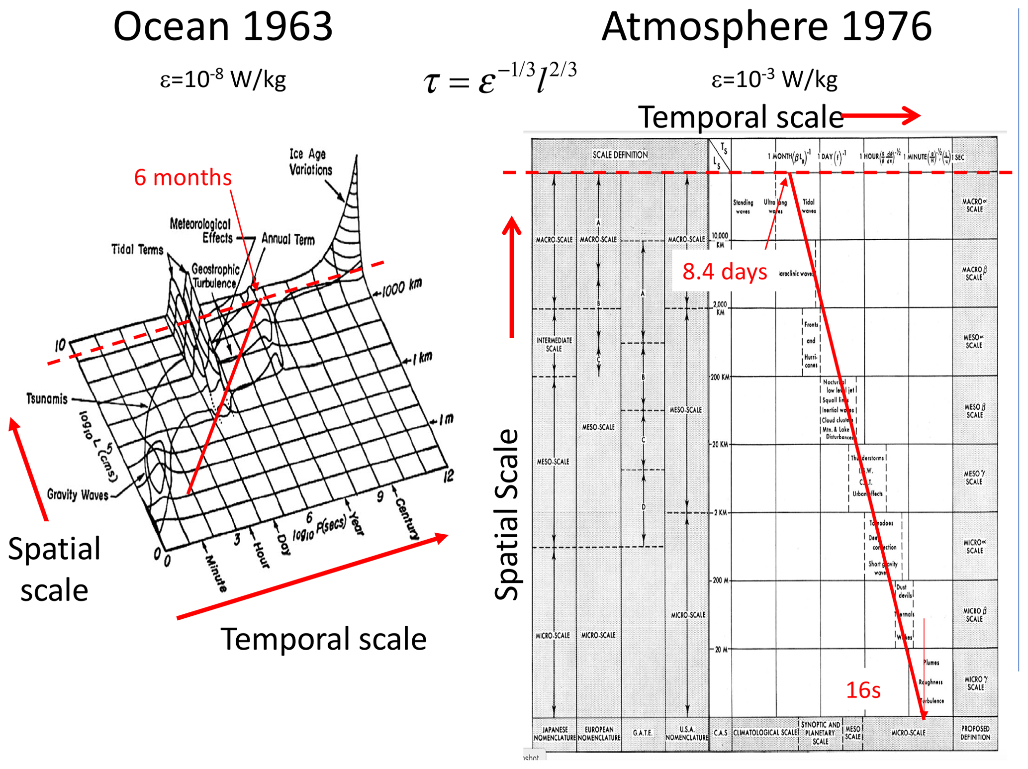
Figure 20The original space–time diagrams (Stommel, 1963, ocean, left; Orlanski, 1975, the atmosphere, right). The solid red lines are theoretical lines assuming the horizontal Kolmogorov scaling with the measured mean energy rate densities indicated. The dashed red lines indicate the size of the planet (half-circumference 20 000 km), where the timescale at which they meet is the lifetime of planetary structures (≈ 10 d in the atmosphere, about 6 months in the ocean). It is equal to the weather–macroweather and ocean weather–ocean macroweather transition scales, and it is also close to the corresponding deterministic predictability limits.
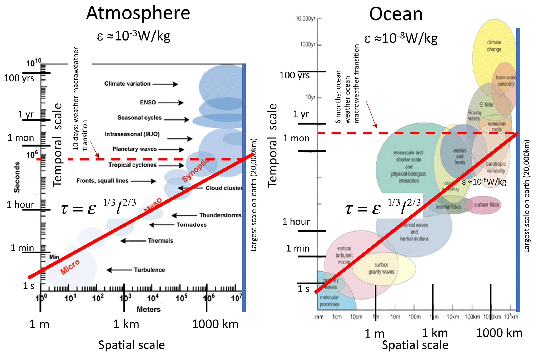
Figure 21The original figures are space–time diagrams for the ocean (left) and atmosphere (right) from Ghil and Lucarini (2020); note that space and time have been swapped as compared to Fig. 20. As in Fig. 20, solid red lines have been added, showing the purely theoretical predictions. On the right, a solid blue line was added showing the planetary scale. The dashed red line (also added) shows the corresponding lifetimes of planetary structures (the same as in Fig. 20). We see once again that wide-range horizontal Kolmogorov scaling is compatible with the phenomenology, especially when taking into account the statistical variability of the space–time relationship itself, as indicated in Fig. 22.
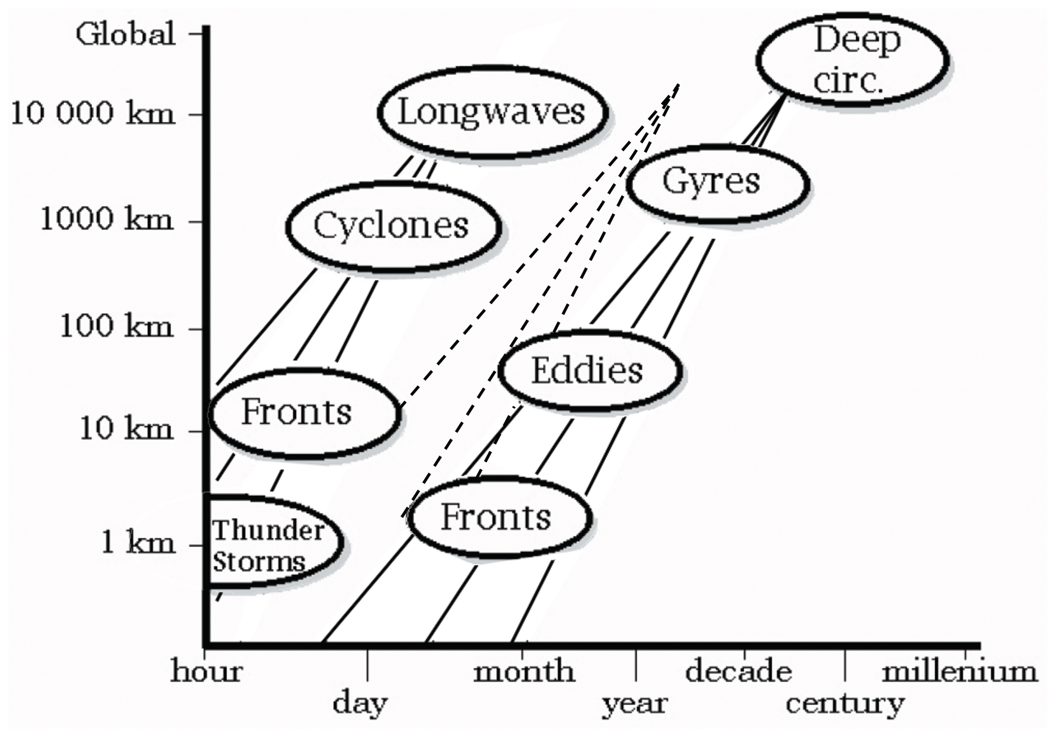
Figure 22A space–time diagram showing the effects of intermittency and, for the oceans, the deep currents associated with very low ε. The original was published in Steele (1995), with solid reference lines added in Lovejoy et al. (2001), and the dashed lines were added in a further update in Lovejoy and Schertzer (2013). The central black lines indicate the mean theory (i.e. with W kg−1 left and right, appropriate for deep water). The central dashed lines (surface layers) represent W kg−1. The lines to the left and right of the central lines represent the effects of intermittency with exponent C1=0.25 (slopes .75 and 0.59; see Sect. 3: this corresponds to roughly 1 standard deviation variation of the singularities in the velocity field). Reproduced from Lovejoy and Schertzer (2013).
2.6.2 The atmosphere as a heat engine: space–time scaling and the weather–macroweather transition scale
Thinking of the atmosphere as a heat engine that converts solar energy into mechanical energy (wind) allows us to estimate ε directly from first principles. Taking into account the average albedo and averaging over day, night, and the surface of the globe, we find that solar heating is ≈ 238 W m−2. The mass of the atmosphere is ≈104 kg m−2, so that the heat engine operates with a total power of 23.8 mW kg−1. However, heat engines are never 100 % efficient, and various thermodynamic models (e.g. Laliberté et al., 2015) predict efficiencies of a few percent. For example, an engine at about 300 K that operates over a range of 12 K has a Carnot efficiency of 4 %.
On Earth, direct estimates of ε from wind gradients (using find large-scale average values of ≈ 1 mW kg−1, implying an efficiency of (1 mW kg−1)(23.8 mW kg−1) ≈ 4 %, confirming the theory (Lovejoy and Schertzer, 2010c) (the values 1 mW kg−1 and 23.8 mW kg−1 are for global averages, there are systematic latitudinal variations, and Fig. 23 confirms that the theory works well at each latitude).
Using the value ε≈1 mW kg−1 and the global length scale Le gives the maximum lifetime τ≈10 d (this is where the lines in the Stommel diagrams intersect the Earth scales in the atmospheric Stommel diagrams). For the surface ocean currents, as reviewed in Chap. 8 of Lovejoy and Schertzer (2013), ocean drifter estimates yield ε≈ 10−8 W kg−1, implying a maximum ocean gyre lifetime of about 6 months to 1 year. Deep ocean currents have much smaller values –10−15 W kg−1 (or less) that explain the right-hand side of the Stommel diagram (Fig. 22). This diagram indicates these values, with the theoretical slope fitting the phenomenology well. The figure also shows the effect of intermittency (Sect. 3.3) that implies a statistical distribution about the exponent (this is simply the exponent of the mean), the width of which is also theoretically estimated and shown in the plot, thus potentially explaining the statistical variations around the mean behaviour.
In space, up to planetary scales, the basic wind statistics are controlled by ε; hence, up to τw, they also determine the corresponding temporal statistics. Beyond this timescale, we are considering the statistics of many planetary-scale structures. That the problem becomes a statistical one is clear since the lifetime in this anisotropic 23/9D turbulence is essentially the same as its predictability limit, the error-doubling time for the l-sized eddies (e.g. Chap. 2 of Lovejoy and Schertzer, 2013). If the atmosphere had been perfectly flat (or “layerwise flat” as in quasi-geostrophic 2D turbulence), then its predictability limit would have been much longer (e.g. Chap. 2 of Lovejoy and Schertzer, 2013). Therefore, at this transition scale, even otherwise deterministic GCMs become effectively stochastic. Since the longer timescales are essentially large-scale weather, this has been dubbed “macroweather”.
Figure 24 shows atmospheric and oceanic spectra clearly showing the weather–macroweather transition and ocean weather–ocean macroweather transitions at the theoretically calculated timescales. It also shows the only other known weather–macroweather transition, this time on Mars using Viking lander data. The Martian transition time may be theoretically determined by using the Martian value ε≈40 mW Kg−1 and a 4 % Carnot efficiency. Using the Martian solar insolation and atmospheric mass, the theory predicts a Martian weather–macroweather transition at about 1.8 sols (1 sol ≈ 25 h), a prediction confirmed in Fig. 24 (Lovejoy et al., 2014).
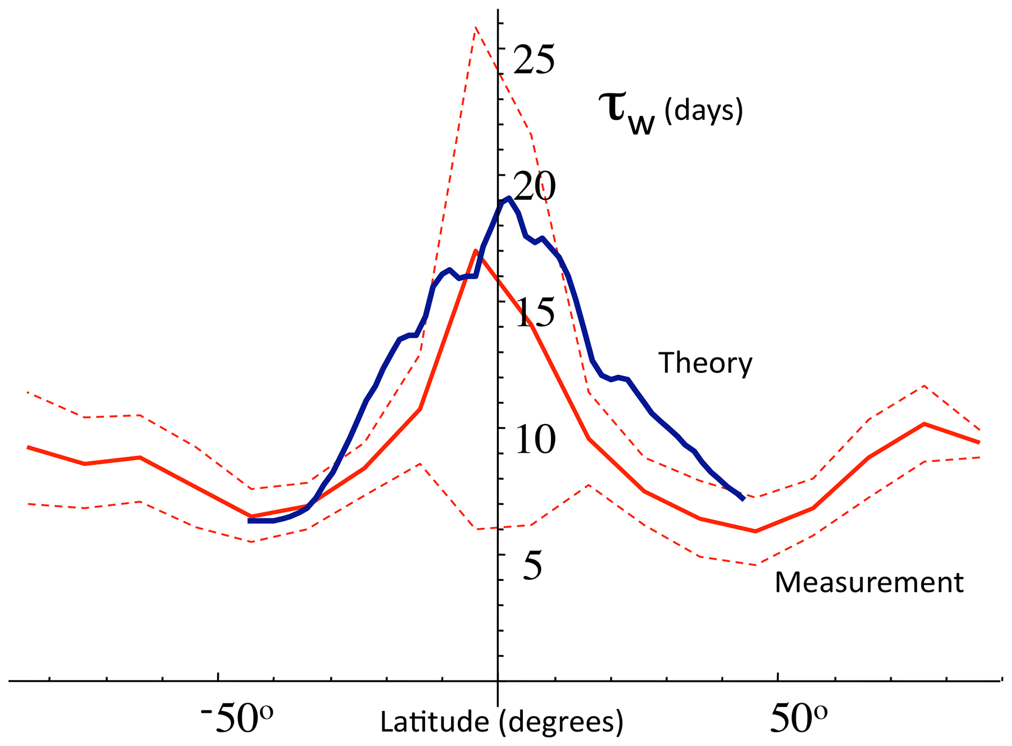
Figure 23The weather–macroweather transition time τw as a function of latitude. Blue shows the theoretical curve (±45∘ latitude only) estimated from the horizontal wind field at 700 mb (blue, using and data from the ECMWF reanalysis) and red direct estimates from breaks in the spectra of 700 mb temperature series at 2∘ resolution from the 20th century reanalysis (the solid line is the mean and the dashed lines are the 1 standard deviation spread along each latitude line). Adapted from Lovejoy and Schertzer (2013).
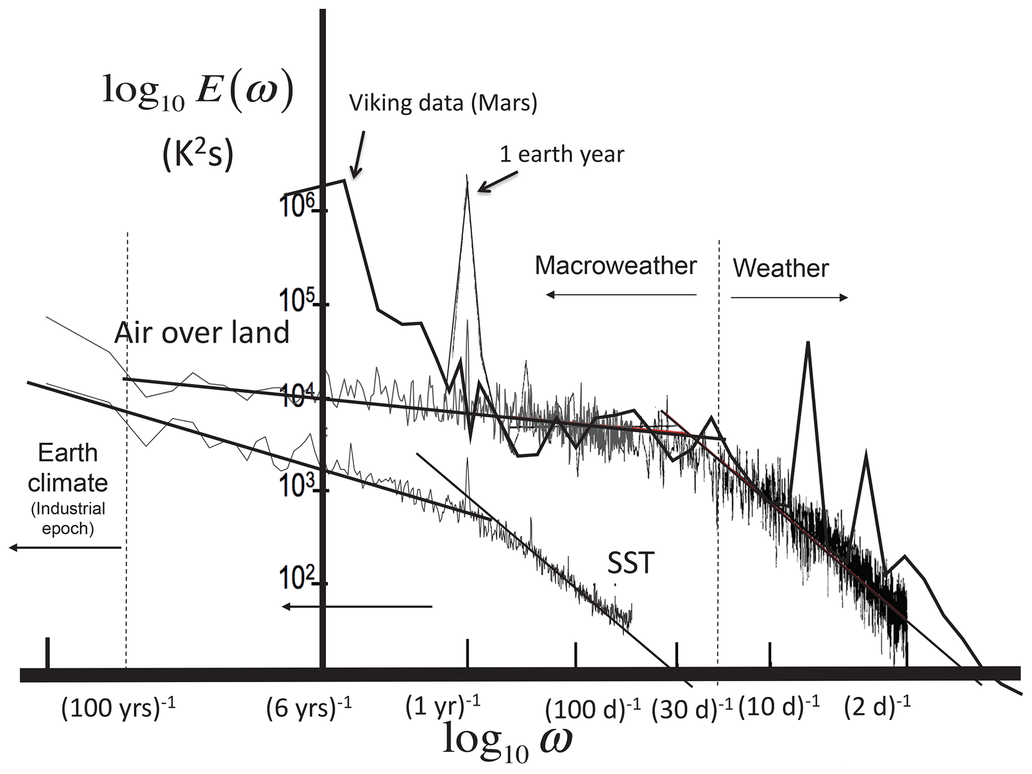
Figure 24The three known weather–macroweather transitions: air over the Earth (black, and upper left, grey), the sea surface temperature (SST, ocean) at 5∘ resolution (lower line, thin black), and air over Mars (thick, solid, black). The air over the Earth's curve is from 30 years of daily data from a French station (Macon, black) and from air temperatures for the last 100 years (5∘ × 5∘ resolution NOAA NCDC), and the spectrum of monthly averaged SST is from the same database. The Mars spectra are from Viking lander data. The strong “spikes” on the right are the Martian diurnal cycle and its harmonics. On the far left, the spectral rise (Earth) is the low-frequency response to anthropogenic forcing. Reproduced from Lovejoy (2019).
2.7 Eulerian space–time relations
In the previous section, we discussed the space–time relations of structures of size l that maintained their identities over a lifetime τ – these space–time diagrams are Lagrangian (albeit deduced from Eulerian data and reanalyses). Unsurprisingly, it turns out to be much simpler to empirically check the corresponding fixed-frame Eulerian relations; we consider this in this subsection.
The key difference between the Eulerian and Lagrangian statistics is that the former involves an overall mean advection velocity V. When studying laboratory turbulence, Taylor (1938) proposed that the turbulence is “frozen”, such that the pattern of turbulence blows past the measuring point sufficiently quickly so that it does not have time to evolve. Frozen turbulence requires the existence of a scale separation between small and large scales, so that the large (nearly frozen) structures really do blow the small ones' structures without much evolution. When this approximation is valid, the spatial statistics may be obtained from time series by the deterministic transformation VΔt→Δx, where V is a constant.
In Taylor's laboratory turbulence, V is determined by the fan and by the wind-tunnel geometry, and within limits, the approximation is valid. However, although the transformation has been frequently used to interpret meteorological data, due to the horizontal scaling, there is no scale separation between large and small scales, so that atmospheric turbulence is not frozen. However, we are only interested in the statistical relations between time and space, and if the system is scaling, then advection can be taken into account using the Galilean transformation , t→t. Since V is now a random (turbulent) velocity, its effects must then be averaged; this is discussed in Sect. 4.1.5. The full theory of space–time scaling requires the consideration of anisotropic space–time and was developed in Schertzer et al. (1997a), Lovejoy et al. (2008b), and Pinel et al. (2014) and reviewed in Lovejoy and Schertzer (2013).
In order to test the space–time scaling on real-world data, the best sources are remotely sensed data such as the space–time lidar data discussed in Radkevitch et al. (2008) or the global-scale data from geostationary satellites in the infrared (IR), whose spectra are shown in Fig. 25 (Pinel et al., 2014). The figure uses 1440 consecutive hourly images at 5 km resolution over the region 30∘ N to 30∘ S and 80 to 200∘ E. A full analysis based on the 3D () space data is given in Pinel et al. (2014); the figure shows only 1D subspaces (EW, NS, and time).
There are two remarkable aspects of the figure. The first is that, in spite of an apparently slight curvature (normally a symptom of deviations from perfect scaling), it is in reality largely a “finite-size effect” on otherwise excellent scaling. This can be seen by comparison with the black curve that shows the consequences of the averaging over the (roughly rectangular) geometry of the observing region combined with the “trivial” anisotropy of the spectrum (implied by the matrix C in Eq. 11). This is clearly visible in the various subspaces analysed in Pinel et al. (2014), where the full theory and analysis are given. Comparing the spectra to the theoretical black curve, we see that there are only small deviations from scaling, and this holds over the range in space from 60 km to ≈ 5000 km (space) and from ≈ 2 h to ≈ 7 d.
The second remarkable aspect of Fig. 25 is the near-perfect superposition of the 1D spectra over the same range (obtained by successively integrating out the conjugate variables (e.g. . Writing , the overall result is that the full 3D, horizontal space–time spectrum respects the symmetry: (see Sect. 4.1.5 for the theory). The full relationship between the Lagrangian and Eulerian statistics is derived in full in Pinel et al. (2014) and Chap. 8 of Lovejoy and Schertzer (2013). By averaging over the turbulent advection, the final theoretical result is
where the nondimensional μx and μy are related to the average zonal and meridional advection velocities and their variances, and a is the average “trivial” zonal to meridional aspect ratio. The vertical bars indicate the usual vector norm. Empirically, s=3.4, a≈1.6. Equation (11) implies that the 1D spectra in Fig. 25 respect as shown.
Given the space–time scaling, one can use the real space statistics to define Eulerian space–time diagrams. Using the same data, this is shown in Fig. 26, where we see that the relationship is nearly linear in a linear–linear plot (i.e. with a constant velocity) up to about 10 d, corresponding to near-planetary scales as indicated in the figure. Note some minor differences between the EW and NS directions.
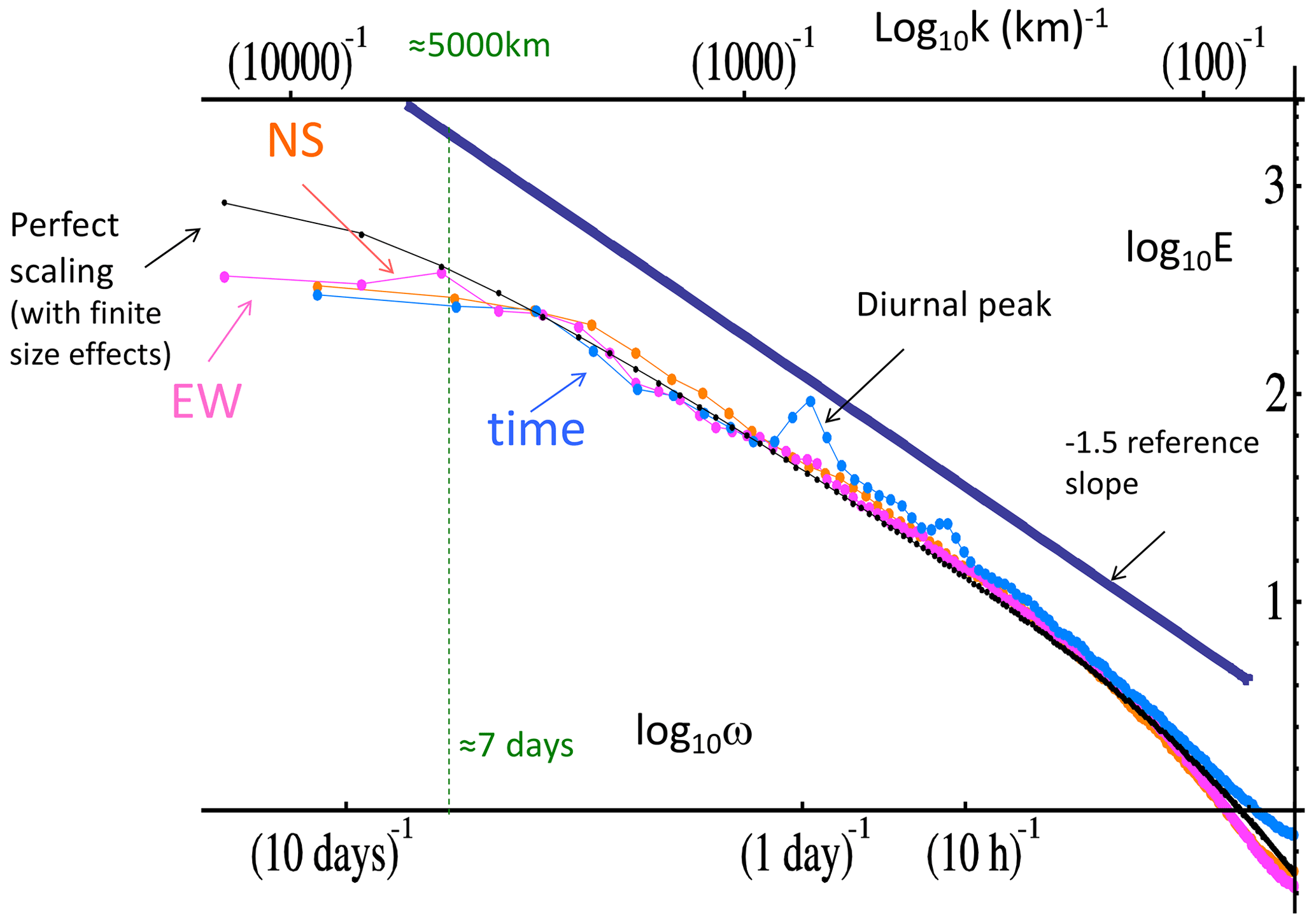
Figure 25The zonal, meridional, and temporal spectra of 1386 images (∼ 2 months of data, September and October 2007) of radiance fields measured by a thermal infrared channel (10.3–11.3 µm) on the geostationary satellite, MTSAT (Multifunctional Transport Satellite), over the south-western Pacific at resolutions 30 km and 1 h over latitudes 40∘ S–30∘ N and longitudes 80–200∘ E. With the exception of the (small) diurnal peak (and harmonics), the rescaled spectra are nearly identical and are also nearly perfectly scaling (the black line shows exact power-law scaling after taking into account the finite image geometry). Adapted from Pinel et al. (2014).
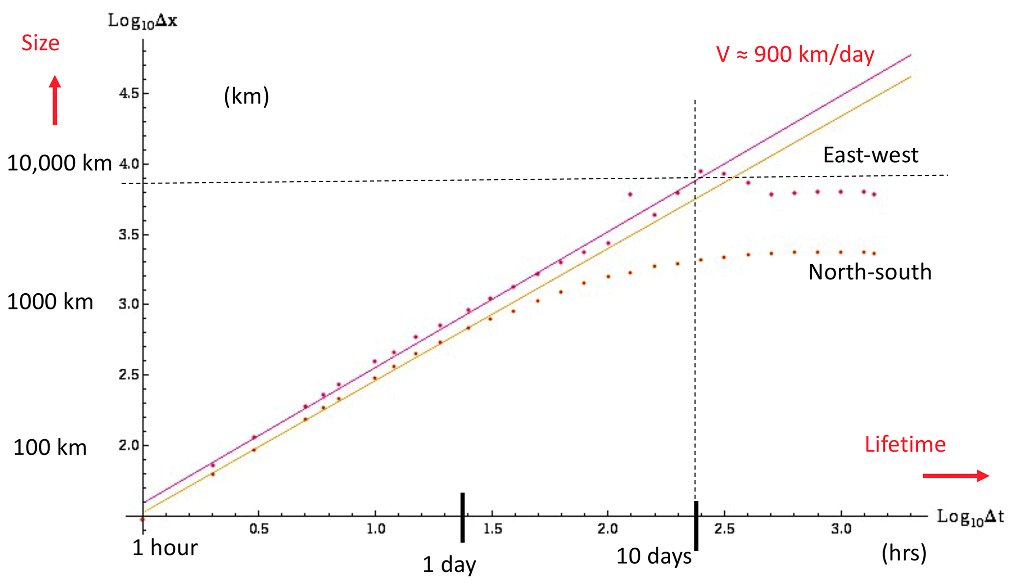
Figure 26The Eulerian (fixed-frame) space–time diagram obtained from the same satellite pictures analysed in Fig. 25, lower left, reproduced from Pinel et al. (2014). The slopes of the reference lines correspond to average winds of 900 km d−1, i.e. about 11 m s−1. The dashed reference lines show the spatial scales corresponding to 1 and 10 d respectively.
3.1 Scaling in one dimension: time series and spatial transects
Up until now, we have discussed scaling at a fairly general level as an invariance under scale changes, contrasting it with scaleboundedness and emphasizing its indispensable role in understanding the atmosphere, the ocean, and, more generally, the geosphere. There are two basic elements that must be considered: (a) the definition of the notion of scale and scale change and (b) the aspect of the system or process that is invariant under the corresponding change (the invariant).
We have seen that, in general terms, a system is scaling if there exists a power-law relationship (possibly deterministic, but usually statistical) between fast and slow (time) or small and large (space, or both, space–time). If the system is a geometric set of points – such as the set of meteorological measuring stations (Lovejoy et al., 1986), then the set is a fractal set and the density of its points is scaling – it is a power law whose exponent is its fractal codimension. Geophysically interesting systems are typically not sets of points but rather scaling fields such as the temperature at the space–time point . Although we will generally use the term scaling “fields”, for multifractals, the more precise notion is of singular densities of multifractal measures.
In such a system, some aspect – most often a suitably defined fluctuation ΔT – has statistics whose small and large scales are related by a scale-changing operation that involves only the scale ratios: the system has no characteristic size. In one dimension the scaling of temporal series or spatial transects can be expressed as
where Δt is the time interval (scale) over which the fluctuations are defined (for transects, replace Δt by the spatial interval Δx), H is the fluctuation exponent, and φΔt is a random variable at resolution ϕΔt. Dimensionally, the units of φ determine H, and physically φ is a turbulent flux that drives the process (or a power of a flux; see Eq. 2). In turbulence theory, (in the relevant “direct” cascades) the fluxes are in Fourier space from small to large wavenumbers. The subscript Δt indicates that φ generally depends on the scale (resolution). The equality sign is in the sense of random variables; this means that the random fluctuation ΔT(Δt) has the same probability distribution as the random variable φΔtΔtH. We suppressed the t dependence since we consider the case where the statistics are independent of time or space – statistical stationarity or statistical homogeneity (see Appendix B4). Physically, this is the assumption that the underlying physical processes are the same at all times and everywhere in space. Equation (12) is the more formal expression of Eq. (1) or of the classical turbulence laws Eq. (4). For example, if we consider space rather than time, the Kolmogorov law has with .
The simplest case is where the fluctuations in a temporal series T(t) follow Eq. (12) but with φ a random variable independent of resolution: , with φ the same as in Eq. (12): a Gaussian random variable. This is the classical special case of non-intermittent, quasi-Gaussian turbulence. Examples are fractional Gaussian noise (fGn, ) and fractional Brownian motion (fBm, ), with special cases Gaussian white noise () and standard Brownian motion ().
Equation (12) relates the probabilities of small and large fluctuations; it is usually easier to deal with the deterministic equalities that follow by taking qth-order statistical moments of Eq. (12) and then averaging over a statistical ensemble:
where “〈〉” indicates statistical (ensemble) averaging.
Equation (13) is the general case where the resolution Δt is important for the statistics of φ; indeed, quite generally, φΔt is a random function (1D) or field averaged at resolution Δt. If φΔt is scaling, its statistics will follow:
where τ is the largest, “outer” scale of the scaling regime satisfied by the equation, and the Δt resolution is λ times smaller. K(q) is a convex (K′′ (q)≥0) exponent function; since the mean fluctuation is independent of the scale (), we have K(1)=0 (see Eq. 2). This is the generic statistical behaviour of cascade processes: it displays general “multiscaling” behaviour – a different scaling exponent K(q) for each statistical moment q. Since large q moments are dominated by large, extreme values and small q moments by common, typical values, K(q)≠0 implies that fluctuations of various amplitudes change scale with different exponents – multiscaling – and each realization of such a process is a multifractal. In general, K(q)≠0 is associated with intermittency, a topic we treat in more detail in Sect. 3.2 and 3.3.
Combining Eqs. (13) and (14), we obtain
where Sq is the qth-order (“generalized”) structure function and ξ(q) is its exponent defined in Eq. (15). Since K(q) is convex, Eq. (15) shows that, in general, ξ(q) will be concave (). The structure functions are scaling since the small and large scales are related by a power law:
As discussed in Sect. 2.3, the spectra are power laws with the exponents related as (Eq. 9).
In the case of “simple scaling” where φ has no scale dependence (e.g. fGn, fBm), we find , where Bq is a constant independent of scale Δt, and hence we have K(q)=0 and Sq(Δt)∝ΔtqH, so that
i.e. ξ(q) is a linear function of q. Simple scaling is therefore sometimes called “linear scaling”, and it respects the simpler relation . Linear scaling arises from scaling linear transformations of noises; the general linear scaling transformation is a power-law filter (multiplication of the Fourier transform by ω−H) or, equivalently, fractional integrals (H>0) or fractional derivatives (H<0). Appropriate fractional integrals of Gaussian white noises (of order ) yield fBm () and fractional derivatives yield fGn (). The analogous Lévy motions and noises are obtained by the filtering of independent Lévy noises (in this case, ξ(q) is only linear for ; for q>α, the moments diverge, so that both ξ(q) and Sq→∞).
The more general “nonlinear scaling” case, where K(q) is nonzero and convex, is associated with fractional integrals or derivatives of scaling multiplicative (not additive) random processes (cascades, multifractals). These pure multiplicative processes (φ in Eq. 12) have H=0, and they are sometimes called “conservative multifractals” since their exponent of the mean is (i.e. the mean is independent of scale). The exponent H in Eq. (15) still refers to the order of fractional integration (H>0) or differentiation (H<0) of φ that adds the extra term qH in the structure function exponent: . Note that while the symbol H is in honour of Edwin Hurst, the interpretation of H as the “Hurst exponent” is only valid for Gaussian processes: more generally, it is a fluctuation exponent describing the behaviour of the mean (q=1) fluctuations.
Note that, in the literature, the notation “H” is not used consistently. It was introduced in honour of Edwin Hurst, a pioneer of long-memory processes sometimes called “Hurst phenomena” (Hurst, 1951). Hurst introduced the rescaled range exponent, notably in the study of Nile River streamflow records. To explain Hurst's findings, Mandelbrot and Van Ness (1968) developed Gaussian scaling models (fGn, fBm) and introduced the symbol H. At first this represented a Hurst exponent, and they showed that, for fGn processes, it was equal to Hurst's exponent. However, by the time of the landmark Fractal Geometry of Nature (Mandelbrot, 1982), the usage was shifting from a scaling exponent to a model specification: the “Hurst parameter”. In this new usage, the symbol H was used for both fGn and its integral fBm, even though the fBm scaling exponent is larger by 1. To avoid confusion, we will call it HM. Subsequently, a mathematical literature has developed using HM with to parameterize both the process (fractional Gaussian motion – fBm) and its increments (fGn). However, also in the early 1980s (Grassberger and Procaccia, 1983; Hentschel and Procaccia, 1983; Schertzer and Lovejoy, 1983b), much more general scaling processes with an infinite hierarchy of exponents – multifractals – were discovered, clearly showing that a single exponent was not enough. Schertzer and Lovejoy (1987) showed that it was nevertheless possible to keep H in the role of a mean fluctuation exponent (originally termed a cascade “conservation exponent”). This is the sense of the H exponent discussed here. As described above, using appropriate definitions of fluctuations (i.e. by the use of an appropriate wavelet), H can take on any real value. When the definition is applied to fBm, it yields the standard fBm value H=HM, yet when applied to fGn, it yields .
We could mention that, here and in Sect. 3.3, where we discuss the corresponding multiscaling probability distributions, we use the c(γ), K(q) codimension multifractal formalism that is appropriate for stochastic multifractals (Schertzer and Lovejoy, 1987). Another commonly used multifractal formalism is the α, f(α), τ(q) dimension formalism of Halsey et al. (1986) that was developed for deterministic chaos applications. The relationship between the two formalisms is , where d is the dimension of the space in which the multifractal process is defined and is the singularity of the measure of the multifractal – not its density, whose singularity is γ. For the moment exponent functions, we have .
The α, f(α), and τ(q) “dimension” formalism was developed to characterize deterministic chaos in low-dimensional (i.e. small d) spaces. Here we are interested in stochastic multifractal processes that are defined on probability spaces with d=∞. Therefore, a codimension formalism that is independent of d is required. Another difference between the formalisms is that the singularity of the multifractal measure α is assumed to be defined at a mathematical point (it is a “Holder exponent”), whereas in the codimension formalism, γ is the singularity of the density of the multifractal measure, and only a looser convergence in the neighbourhood of a point is assumed. This lack of pointwise convergence of the singularities is a general feature of (stochastic) cascade processes and hence the codimension formalism is more relevant in the atmosphere.
3.2 Spikiness, intermittency, and multifractals
3.2.1 Spikes, singularities, and codimensions
Atmospheric modelling is classically done using the deterministic equations of thermodynamics and continuum mechanics. However, in principle, one could have used a more fundamental (lower-level) approach – statistical mechanics – but this would have been impossibly difficult. However, in strongly nonlinear fluid flow, the same hierarchy of theories continues to higher-level turbulent laws. These laws are scaling and may – depending on the application – be simpler and more useful. A concrete example is in the macroweather regime where (strongly nonlinear, deterministic) GCMs are taken past their deterministic predictability limit of about 10 d. Due to their sensitivity to initial conditions, there is an inverse cascade of errors (Lorenz, 1969; Schertzer and Lovejoy, 2004), so that, beyond the predictability limit, small-scale errors begin to dominate the global scales, so that the GCMs effectively become stochastic. To some degree of approximation, since the intermittency is low (the spikiness on the right-hand side of Fig. 2 and at the bottom of Fig. 3), this stochastic behaviour is amenable to modelling by linear stochastic processes, in this case, the half-order and fractional energy balance equations (HEBE, FEBE, Lovejoy, 2021a, b; Lovejoy et al., 2021; Lovejoy, 2022c). The key issue – of whether linear or nonlinear stochastic processes can be used – thus depends on their “spikiness” or intermittency (multifractality).
Classically, intermittency was first identified in laboratory flows as “spottiness” (Batchelor and Townsend, 1949) in the atmosphere by the concentration of atmospheric fluxes in tiny, sparse regions. In time series, it is associated with turbulent flows undergoing transitions from “quiescence” to “chaos”. Quantitative intermittency definitions developed originally for fields (space) are of the “on–off” type, the idea being that when the energy or other flux exceeds a threshold, then it is “on”, i.e. in a special state – perhaps of strong/violent activity. At a specific measurement resolution, the on–off intermittency can be defined as the fraction of space where the field is “on” (where it exceeds the threshold). In a scaling system, for any threshold, the “on” region will be a fractal set and both the fraction and the threshold will be characterized by exponents (by c and γ, introduced shortly) that describe the intermittency over all scales and all intensities (thresholds). In scaling time series, the same intermittency definition applies; note however that other definitions are sometimes used in series in deterministic chaos.
With the help of multifractals, we can now quantitatively interpret the spike plots. Recall that (Eq. 12), where φΔt is the flux driving the process at resolution Δt and normalized so that 〈φΔt〉=1. If we estimate the ensemble mean flux by the (temporal) average flux over the entire time series and then average the result over all the available series (indicated by an overbar), then and the normalized spikes are estimates of the nondimensional, normalized driving fluxes:
where φΔt,un is the raw, unnormalized flux, and the outer scale of the scaling regime is τ, so that the normalized flux φλ is over the scale ratio λ. In the weather regime in respectively time and space, the squares and cubes of the wind spikes are estimates of the turbulent energy fluxes. This spikiness is because most of the dynamically important events are sparse and hierarchically clustered, occurring mostly in storms and at the centre of storms.
As long as H<1 (true for nearly all geo-processes), the differencing that yields the spikes acts as a high-pass filter, and the spikes are dominated by the high frequencies. Smoothed Gaussian white noises such as the scaling fGn and fractional Brownian motion (fBm) processes or non-scaling processes such as autoregressive and moving average processes will have spikes that look like the weak macroweather spikes in Fig. 2, roughly bounded by the solid horizontal line in the figure.
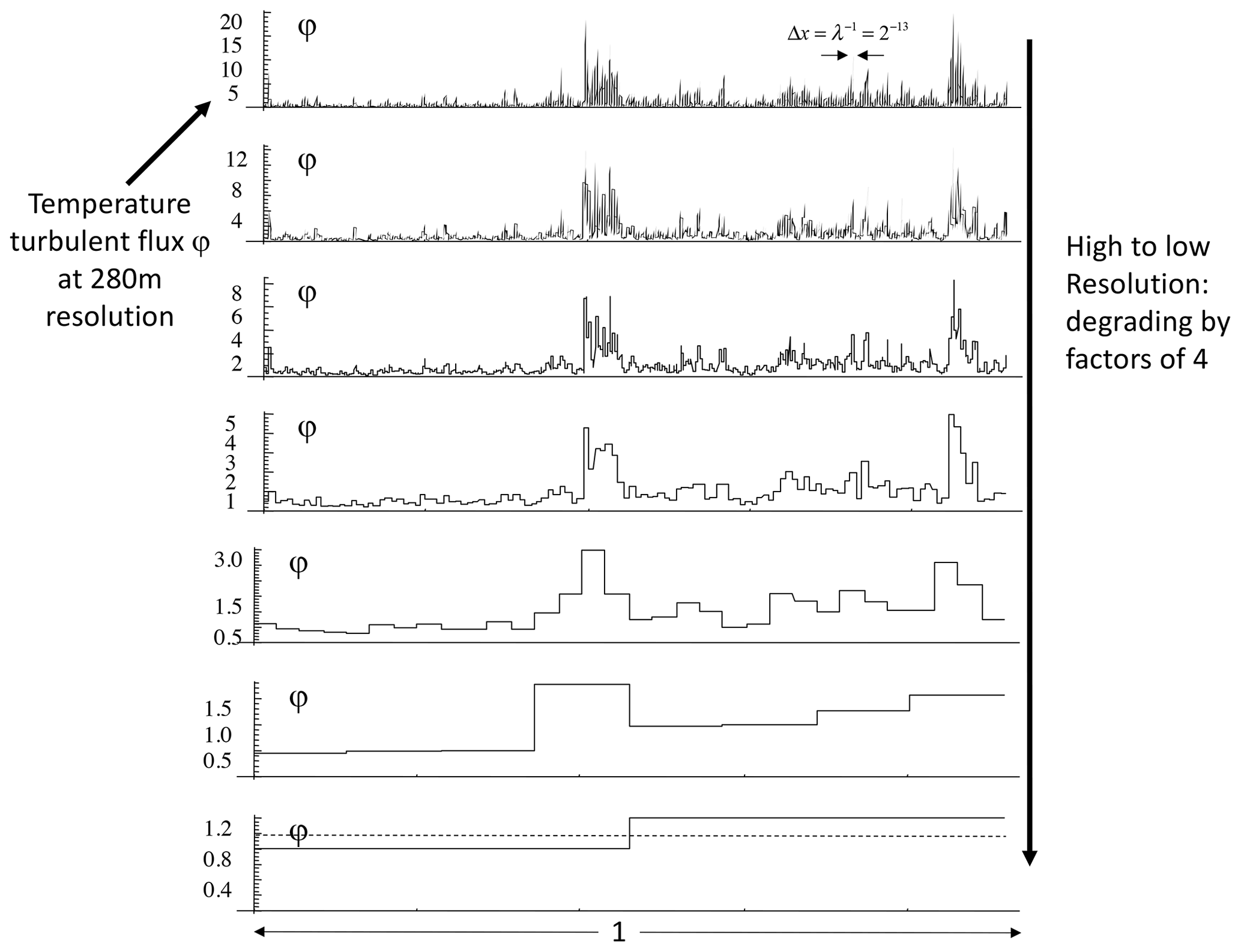
Figure 27The top row is a reproduction of the intermittent spikes taken from the gradients in the aircraft data at the bottom of Fig. 3. The original series is 2294 km long with resolution 280 m, and hence it covers a scale range of a factor of λ=213. Here we use nondimensional units, so that the length is 1 with resolution . Moving from top to bottom, each row degrades (by averaging) the resolution of the previous one by a factor of 4. Note that the scale on the left is constantly changing. At the bottom, the dashed line indicates the mean, which is unity since φ is a normalized process. Reproduced from Lovejoy (2019).
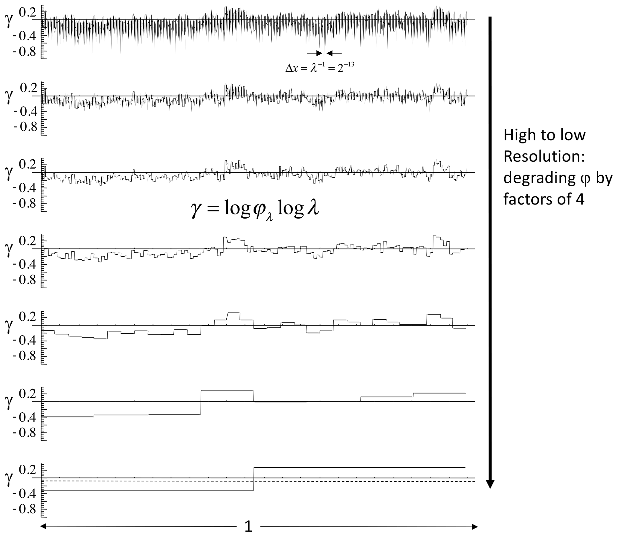
Figure 28The same as Fig. 27 but in terms of the corresponding singularities obtained through the transformation of variables . Note that, while the range of variation of the φ in the previous figure rapidly diminishes as the resolution is lowered, by contrast, the amplitude of the fluctuations of the γ values (above) is roughly the same at all scales. Note that the dashed horizontal line in the bottom plot shows the mean singularity, here −0.06. It is <0 since it is the mean of the log of the normalized flux and the logarithm function is concave. Adapted from Lovejoy and Schertzer (2013).
What happens if we change the resolution of φλ by averaging it over larger and larger scales Δt (smaller λ)? Figure 27 shows this using the example of the spatial (aircraft) transect in Fig. 3. The top plot is identical to the bottom of Fig. 3, except that nondimensional units are used, so that the top spike transect φλ has length 1 with 8192, where L=2294 km is the actual length and Δx=280 m is the transect resolution. As we move from top to bottom, the resolution is successively degraded by factors of 4 (λ decreases by factors of 4). Since the flux is normalized by its mean (λ=1), the fluctuations are about unity (the dashed line at the bottom where λ=2).
Examine now the vertical axes. We see that – as expected – the amplitude of the spikes systematically decreases with resolution, and the plots are clearly not scale-invariant. We would like to have a scale-invariant description of the spikes and a scale-invariant probability distribution of the spikes. For this, each spike is considered to be a singularity of order γ:
This is simply a transformation of variables from the spikes to singularities . Figure 27 shows the same spikes but now in terms of the orders of singularity. Now we see that the vertical range is pretty much independent of the resolution. It is therefore plausible that the characterization of the spikes by γ is scale-invariant. To obtain a scale-invariant characterization of the probabilities, introduce the codimension function c(γ); the spike probability distribution may be written as
is the probability that a randomly chosen normalized spike will exceed a fixed threshold s (it is equal to one minus the more usual cumulative distribution function), and P(s) is a non-scaling prefactor that depends on s and weakly on γ. For data analysis purposes, the P(s) prefactor is inconvenient. Although it can be handled – and c(γ) estimated directly by using the probability distribution multiple-scaling technique (Lavallée et al., 1991) – it is often easier to analyse the statistical moments using trace-moment analysis.
To leading order (i.e. setting the prefactor ≈1), we obtain
We see that, while γ gives a scale-invariant characterization of the spikes, c(γ) does the same for the probability distributions. c(γ) characterizes sparseness because it quantifies how the probabilities of spikes of different amplitudes change with resolution λ. c(γ) corresponds to the sparse set of spikes that exceed the threshold s=λγ. Increasing the spike amplitude (λγ) defines a sparse exceedance set with large c. A series is intermittent whenever it has spikes with c>0.
In the general scaling case, the set of spikes that exceed a given threshold form a fractal set whose sparseness is quantified by the fractal codimension , where d is the dimension of the space (d=1 for series and transects) and D(γ) is the corresponding fractal dimension. The codimension is fundamental since it is the exponent of the probability distribution.
Gaussian series are not intermittent since c(γ)=0 for all the spikes. To see this, note that for Gaussian processes the cumulative probability of a spike exceeding a fixed threshold s is independent of the resolution λ, , where here P(s) is related to the error function. Comparing this with Eq. (20), we see that c=0.
Returning to Fig. 2, we have λ=1000. The extreme spikes ( in this 1000-point-long series have a probability . For Gaussian processes, the spikes with this probability are (calculated from the error function). This is shown by the solid lines in Fig. 2: the line therefore corresponds to . If the series in Fig. 2 were generated by multifractal processes, what is the maximum γ (and hence spike) that we would expect? The extreme value would still correspond to λ−1; hence, from Eq. (20), we have . More generally, in a space of dimension d, there would be λd spikes, and the probability of the maximum would be λ−d, so that . Since the fractal dimension of the spikes is , this is simply the result that . Since c(γ) is a monotonically increasing function, this is just the simple geometric result that the fractal dimension of the exceedance sets cannot be negative. Appendix A, Table 2 gives both the observed maximum γ for each series in Fig. 2 and the generally comparable theoretically expected maxima for the multifractal processes with the parameters estimated for the series in question.
While c(γ) quantifies the way the probability distributions of spikes change with scale, the moment-scaling exponent K(q) (Eq. 14) quantifies the way the statistical moments change with scale. Since the process can be equivalently characterized by either probabilities or moments, c and K must be related. Indeed, the relationship is beautiful and simple, via a Legendre transformation
(Parisi and Frisch, 1985).
These equations imply one-to-one relationships between the spike singularities γ (and amplitudes λγ) and the exponent of the order of moments q; they imply and . is therefore the singularity that gives the dominant contribution to the mean (q=1) of the process. At the same time, K(1)=0, so that (Eq. 22) (where γ1 is the value that gives the maximum of γ−c(γ)) and so that we obtain γ1=c(γ1), and since , we have ). Defining C1=c(γ1) as the codimensions of the singularity γ1 that gives the dominant contribution to the mean, we have . Thus C1 plays the dual role of being the order of singularity that gives the dominant contribution to the mean while also being equal to the codimension of the set of the corresponding singularities. Since we see that ), this justifies the interpretation of C1=γ1 as the codimension of the mean.
3.2.2 Universal multifractals
At first sight, general (multifractal) scaling involves an entire exponent function – either K(q) or c(γ) – for its statistical characterization, the equivalent of an infinite number of parameters (e.g. one for each statistical moment). This would be unmanageable – either from the point of view of empirical parameter estimation or from the point of view of model construction. Fortunately, one can avail oneself of a multiplicative version of the central limit theorem, which leads to “universal multifractals” with
and (via Legendre transform, Eq. 22)
(Schertzer and Lovejoy, 1987). C1 is the codimension of the mean introduced earlier, is the Lévy index, and α′ is an auxiliary variable introduced for convenience.
Figures 28 and 29 show the universal K(q), c(γ) functions for various values of α in the relevant range . The lower limit α=0 corresponds to the on–off, “monofractal” “β model” (Novikov and Stewart, 1964; Frisch et al., 1978), where all the fluxes are concentrated on a fractal set with codimension C1 and the upper limit α=2 on the “log-normal” multifractal (Kolmogorov, 1962; Yaglom, 1966). Note that, due to the divergence of moments discussed in Sect. 3.5, the multifractals with the above K(q), c(γ) are only approximately “log-Lévy” (or, when α=2, “log-normal”).
Table 1 shows various empirical estimates relevant to atmospheric dynamics. We see that, generally, and C1≈0.1, the main exception being precipitation. As quantified in Table 1, precipitation is the most strongly intermittent atmospheric field (C1≈0.4), quantitatively confirming the subjective impression of extreme precipitation intermittency. The multifractal properties of precipitation have been the subject of numerous studies. Early analyses include spatial analyses by Tessier et al. (1993), Olsson and Niemczynowicz (1996), de Montera et al. (2009), Verrier et al. (2010), and Veneziano et al. (2006) and temporal analyses by Tessier et al. (1993), Hubert et al. (1993), Ladoy et al. (1993), Harris et al. (1996), De Lima (1998), De Lima and Grasman (1999), Hubert et al. (2002), Kiely and Ivanova (1999), Hubert et al. (2002), Pathirana et al. (2003), Venugopal et al. (2006), Garcia-Marin et al. (2008), Pathirana et al. (2003), Serinaldi (2010), Sun and Barros (2010), and Verrier et al. (2011). There is more discussion of Table 1 in Sect. 3.4.
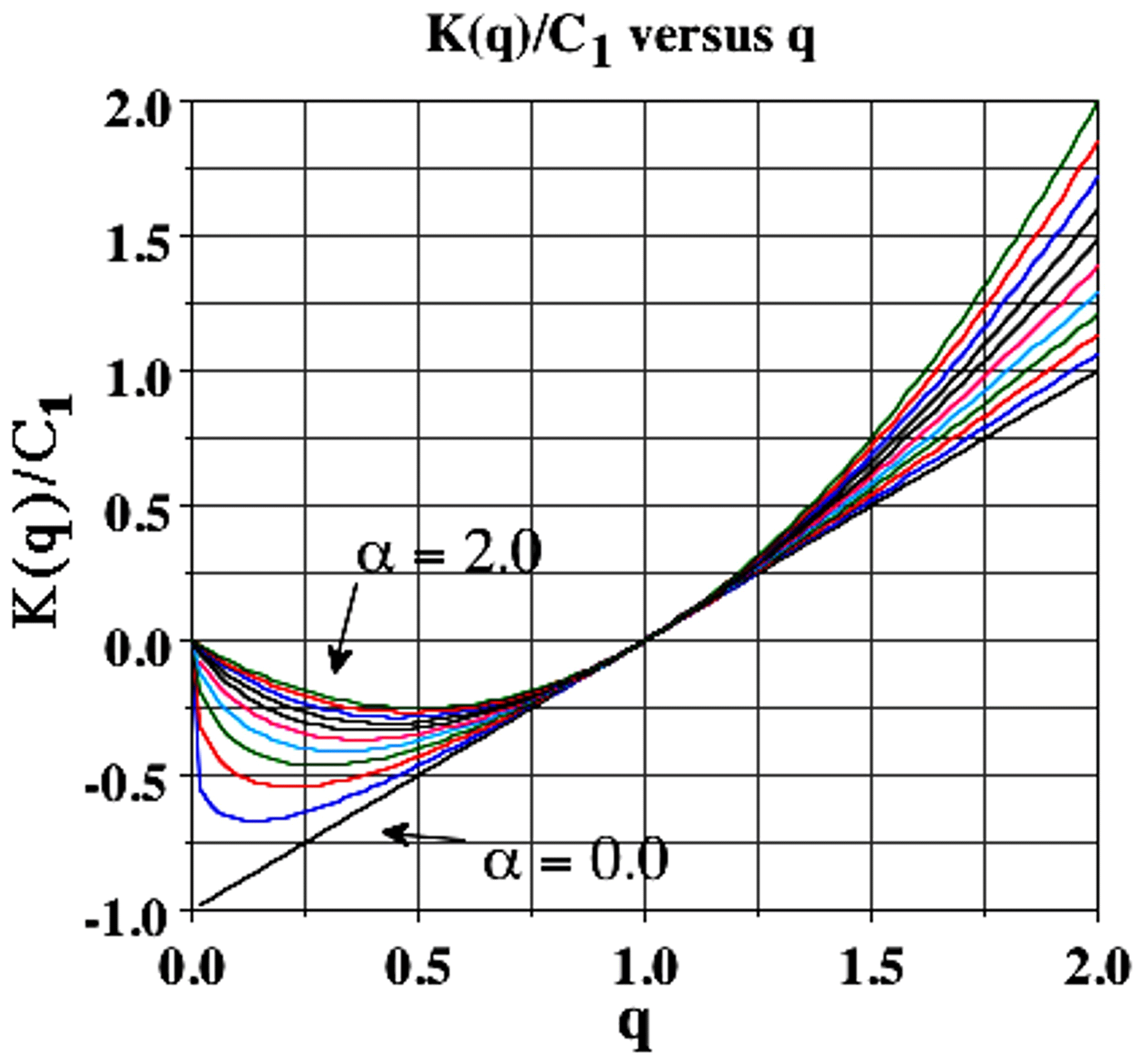
Figure 29Universal K(q) as a function of q for different values from 0 to 2 in increments of 0.2. Adapted from Schertzer and Lovejoy (1989).
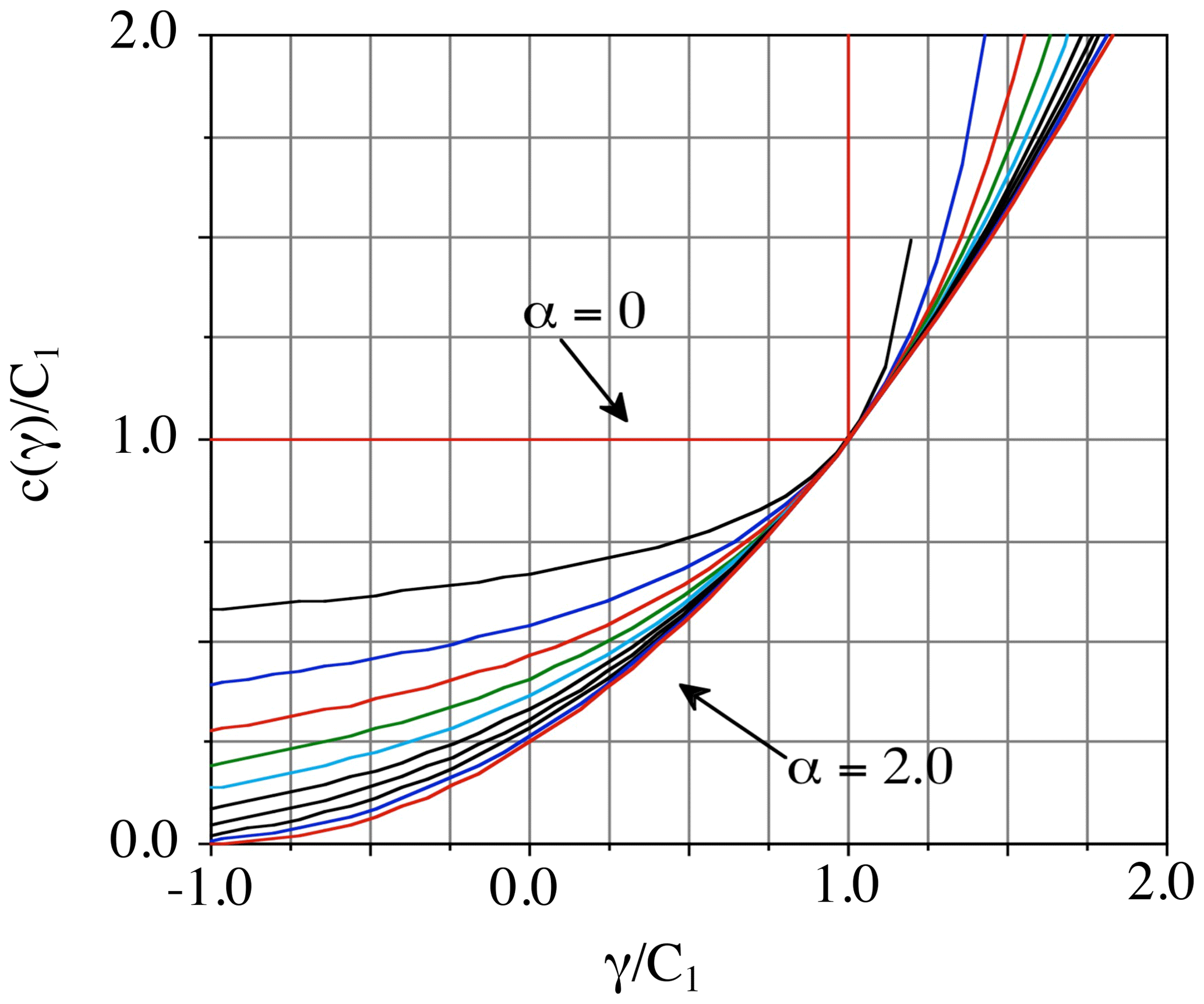
Figure 30Universal c(γ) for α in the range 0 to 2 in increments of 0.2. Adapted from Schertzer and Lovejoy (1989).
Table 1We compare various horizontal parameter estimates, attempting to give summarized categories of values (radiances) or approximate values (u,v, and w are the zonal, meridional, and vertical winds, T the temperature, h the humidity, and z the pressure height). C1 is the codimension of the mean (a convenient intermittency parameter) α, the multifractal index, H the fluctuation exponent, and β the spectral exponent. Leff is the effective outer-cascade scale (determined from the crossing scales of the different moments; this is given in kilometres). When available (and when reliable), the aircraft data were used in precedence over the reanalysis values, with the latter given in parentheses in those cases where there was no comparable in situ value or when it was significantly different from the in situ value. For Leff, where the anisotropy is significant, the geometric means of the north–south and east–west estimates are given; the average ratio is 1.6:1 EW–NS (although for the precipitation rate, the along-track TRMM estimate was used). Finally, the topography estimate of Leff is based on a single realization (one Earth), so that we only verified that there was no obvious break below planetary scales. The aerosol concentration was estimated from the lidar backscatter ratio from the data in Fig. 45.
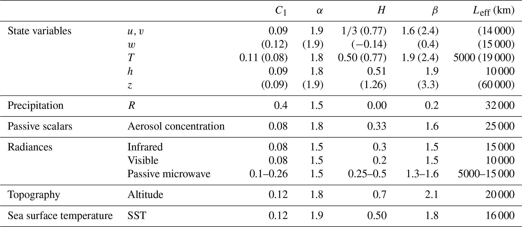
3.3 Quantifying intermittency with structure functions
Using spike plots, we can simply demonstrate the unique character of the macroweather regime: low intermittency in time but high intermittency in space. We introduced the c(γ) function that for each spike level λγ characterizes the probability (fraction) of a transect or series (or more generally space) whose spikes exceed the threshold. In this section we discuss a particularly simple way to analyse the intermittency.
Consider the data shown in Fig. 31 (macroweather time series and spatial transects, top and bottom respectively). Figure 32 compares the rms fluctuations (with exponent ) and the mean fluctuations (with exponent H=ξ(1)) from macroweather temperature time series (bottom) and for the spatial transects (top). When the system is Gaussian (so that K(q)=0), we obtain , so that moments of the mean and rms fluctuations are in a constant ratio. In this case, is parallel to log . Figure 32 (bottom) shows that to a good approximation this is indeed true of the non-spiky temporal series (Fig. 31, top). However, the corresponding statistics of the spatial transect (the top lines in Fig. 31) tend to converge at large Δx corresponding to the highly spiky transect (Fig. 32, bottom). To a first approximation, it turns out that , which characterizes the intermittency near the mean. However, there is a slightly better way to estimate C1, using the intermittency function (see Fig. 33 and caption) whose theoretical slope (for ensemble-averaged statistics) is exactly . As a point of comparison, we could note that fully developed turbulence in the weather regime typically has C1≈0.09. The temporal macroweather intermittency (C1≈0.01) is indeed small, whereas the spatial intermittency is large (C1≈0.12).
For many applications, the exceptional smallness of macroweather intermittency makes the “monoscaling” approximation (i.e. ξ(q)≈Hq) acceptably accurate, so that macroweather processes are relatively easy to statistically characterize. In this case, the fluctuation exponent H, the spectral exponent β, and the DFA exponent a (Appendix A5) are equivalent and sufficient (the general relations are , and here, with no intermittency, K(2)=0, and these simplify to . For examples of macroweather scaling, see Tessier et al. (1996), Pandey et al. (1998), Koscielny-Bunde et al. (1998), Bunde et al. (2004), Eichner et al. (2003), Blender et al. (2006), Huybers and Curry (2006), Rybski et al. (2006), Lennartz and Bunde (2009), Lanfredi et al. (2009), Fraedrich et al. (2009), Franzke (2010, 2012), Varotsos et al. (2013, 2009), and de Lima and Lovejoy (2015).
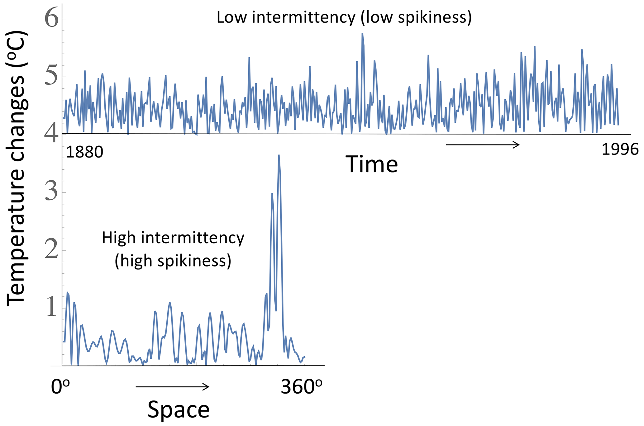
Figure 31A comparison of temporal and spatial macroweather series at 2∘ resolution. The top shows the absolute first differences of a temperature time series at monthly resolution (from 80∘ E, 10∘ N, 1880–1996, displaced by 4 K for clarity), and the bottom is the series of absolute first differences of a spatial latitudinal transect (annually averaged, 1990 from 60∘ N) as a function of longitude. Both use data from the 20CR. One can see that, while the top is noisy, it is not very “spiky”. Quantitatively, the intermittency parameter near the mean is C1≈0.01 (time), C1≈0.12 (space). Reproduced from Lovejoy (2022b).
3.4 Multifractal analyses of geofields: direct (trace-moment) estimates of outer scales and K(q) for Earth and Mars
In the preceding sections, we gave evidence that diverse atmospheric fields are scaling up to planetary scales. In addition, we argued that they generally were multifractal, with each statistical moment q having a different exponent (K(q), Eq. 14). In Sect. 3.2, we saw that this nonlinear, convex part of the structure function exponent ξ(q) arises due to variability building up scale by scale from a large external scale L to smaller scales Δx (ratio or, in time, . By analysing the statistics of the fluxes , this gives us the possibility of directly determining the effective outer scale of the process, i.e. the scale at which the variability starts to grow. As a bonus, our method is based on isolating the flux: in the exponent, it yields K(q) rather than ξ(q) (fluctuations). By effectively removing the qH term, i.e. ξ(q)−K(q), it is only sensitive to K(q), which for small q is often a small correction to ξ(q).
Before proceeding to empirical analyses of the fluxes, a few comments are required. The flux in Eq. (14) is assumed to be normalized, i.e. 〈φλ〉=1. For empirical estimates, one starts with unnormalized fluxes, and one does not know a priori the effective outer scale of the variability L that is needed to estimate the ratio λ. The normalization problem is easy to solve (see Eq. 18). For empirical estimates, one therefore starts with these normalized fluxes at the smallest available resolution (i.e. Δx=1 pixel); using this, lower-resolution estimates (i.e. larger Δx) are obtained simply by averaging. However, to verify Eq. (14), we need the scale ratio λ, which is the ratio of the (a priori unknown) outer scale L to the resolution Δx. The simplest procedure is to use the largest planetary-scale Lref (half the Earth's circumference) as an initial reference scale, a guess hopefully not far from the true outer scale L, a kind of “bootstrap”. When this is done, the statistics of the various moments as functions of the reference-scale ratio (i.e. with in place of are plotted in a log–log plot. For each moment order of q, the regressions with slopes K(q) all converge to the true outer scale; this is because at that scale λ=1, and (Eq. 14) shows that for all q.
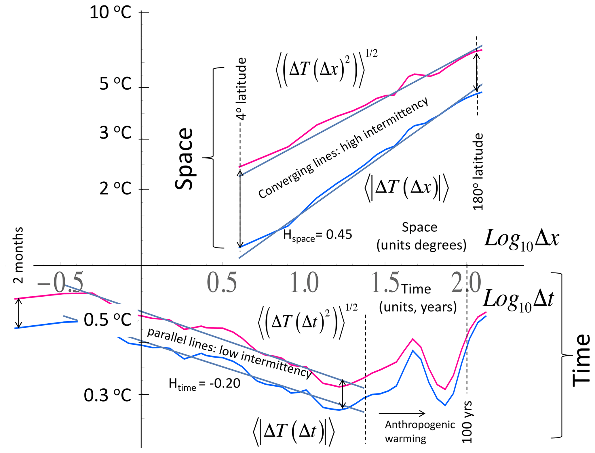
Figure 32The first-order and rms Haar fluctuations of the series and transect in Fig. 31. One can see that, in the spiky transect, the fluctuation statistics converge at large lags (Δx), and the rate of the convergence is quantified by the intermittency parameter C1. The time series (bottom) is less spiky, converges very little, and has low C1 (see Fig. 31, top). The break in the scaling at ≈ 20 years is due to the dominance of anthropogenic effects at longer timescales. Reproduced from Lovejoy (2022b).
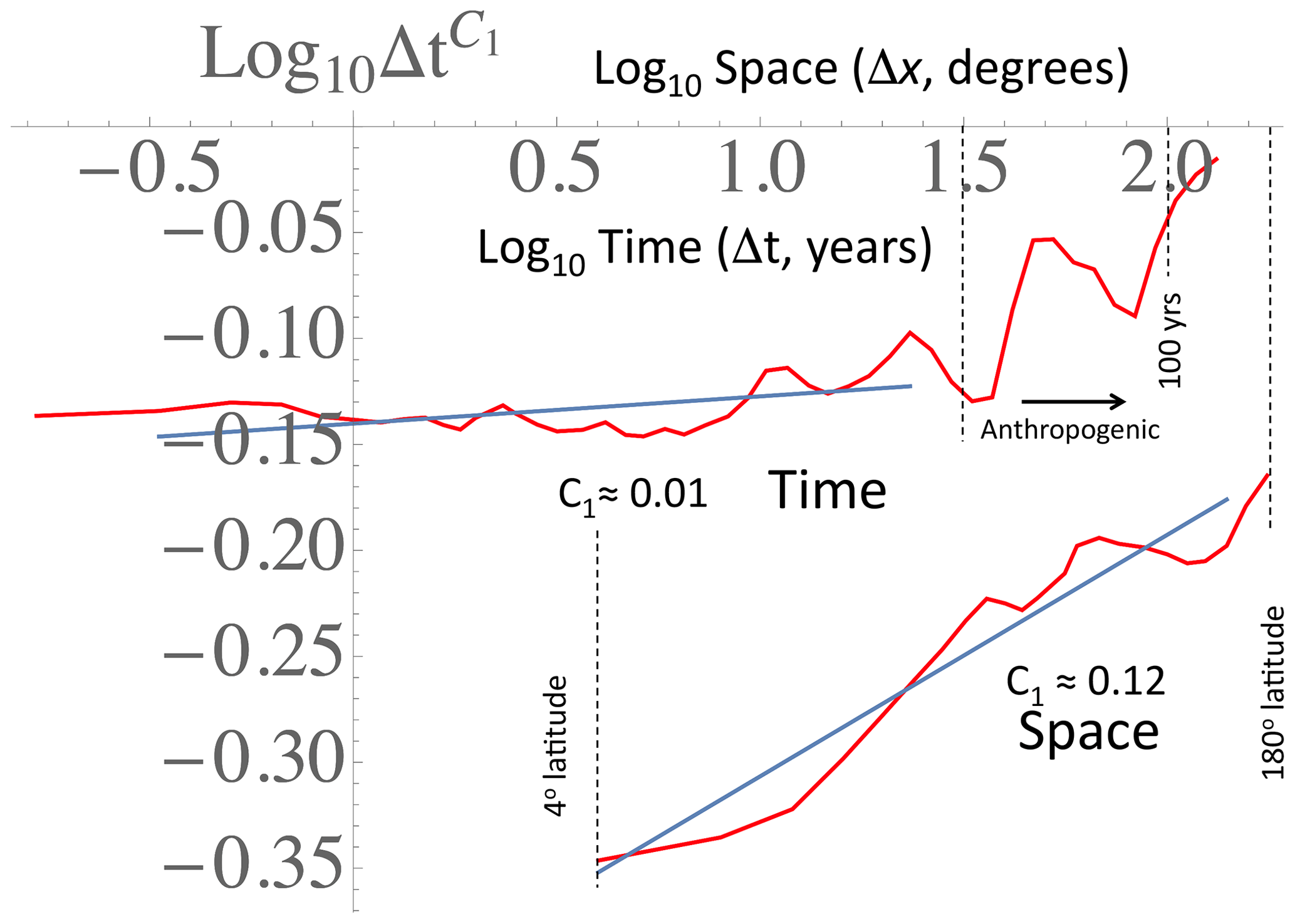
Figure 33A comparison of the intermittency function for the series and transect in Fig. 31, quantifying the difference in intermittencies: in time, C1 ≈ 0.01, and in space, C1 ≈0.12. Since , when Δq is small enough (here, Δq=0.1 was used), we have . The break in the temporal scaling at about 20–30 years (log10Δt≈1.5) is due to anthropogenic forcings. Reproduced from Lovejoy (2022b).
Figure 34 shows the first empirical trace-moment estimate (Schertzer and Lovejoy, 1987). It was applied to data from a land-based radar whose 3 km altitude reflectivity maps were 128 km wide with a 1 km resolution. The vertical axis is Log10Mq, where and , with Lref=128 km. Although this gives a tantalizing hint that atmospheric cascades start at planetary scales, it was not until 20 years later when a decade of satellite radar data was released over the Internet that this was confirmed directly (Fig. 35, Lovejoy et al., 2009e). The poor scalings (curvature) for the low q values (bottom) were quantitatively explained as artefacts of the fairly high minimum detectable signal. Figure 36 shows similar results, but this time using the same geostationary satellite data whose spectra were analysed in Fig. 25. An interesting comparison of horizontal and vertical cascade structures from vertical sections of lidar aerosol backscatter is shown in Fig. 37. Although this is discussed in Sect. 4.1, we can already note that the outer scales are roughly the largest available (≈ 20 000 km in the horizontal and ≈ 10 km in the vertical), but analysis also shows that the slopes K(q) are the theoretically predicted ratio (for all q, Sect. 4).
The trace moments characterize a fundamental aspect of the atmosphere's nonlinear dynamics – its intermittency – in fully developed turbulence, which is expected to be a “universal” feature, i.e. found in all high Reynolds number flows. In our case, the closest universality test is to compare Earth with Mars (using the same reanalyses as in Fig. 9). Figure 38 shows the result when this technique is applied to both terrestrial and Martian reanalyses for pressure, wind, and temperature (for both planets, the reanalyses were at altitudes corresponding to about 70 % of surface pressure). One can note that, (a) as predicted, the turbulence is universal, i.e. not sensitive to the forcing mechanisms and boundaries, so that the behaviour is nearly identical on the two planets, (b) there is clear multiscaling (the logarithmic slopes K(q)≠0), and (c) the effective outer scales (where the lines converge) are indeed nearly the size of the planet. For more detailed discussion and analyses (including spectra and horizontal anisotropy), see Chen et al. (2016).
Table 1 shows typical values of multifractal parameters estimated from trace moments (Sect. 3.4) of various atmospheric fields. Over the decades, many multifractal analyses of geofields have been performed, including of atmospheric boundary conditions, notably the topography on Earth (Lavallée et al., 1993; Gagnon et al., 2006), Mars (Landais et al., 2015), and the sea surface temperature (Lovejoy and Schertzer, 2013). We can see that the universal multifractal index (α) is typically fairly close to the log-normal value (α=2), although due to divergence of moments even when α=2, the statistics of the extremes are power laws (not log-normal; see the next section on divergence of moments). In the table we also see that with the notable exception of the highly intermittent precipitation field, the parameter for the intermittency near the mean (C1) might seem small. However, it should be noted that since the cascades operate over huge ranges of scales, the resulting fields are nevertheless highly intermittent. In addition, it should be recalled that, since α≈2, the intermittency increases very rapidly for the higher-order moments; so, for example, the kurtosis (q=4) has an “effective” intermittency 12 times larger (K(4)=C1 (42−4) = 12C1).
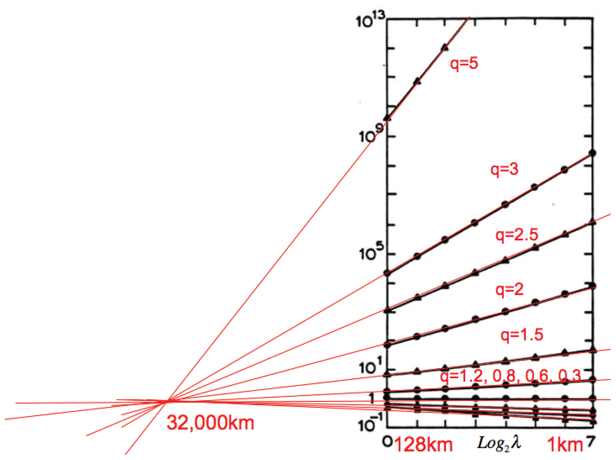
Figure 34The moments of the normalized radar reflectivity factor for 70 constant-altitude radar maps at 3 km altitude from the McGill weather radar (10 cm wavelength). As can be seen, the outer scale (where the lines cross) is at roughly 32 000 km. This scale is a bit larger than the Earth's half-circumference because even at the largest scale there is some precipitation variability due to the interaction of precipitation with the other atmospheric fields. From Schertzer and Lovejoy (1987), adapted in Lovejoy et al. (2008a).
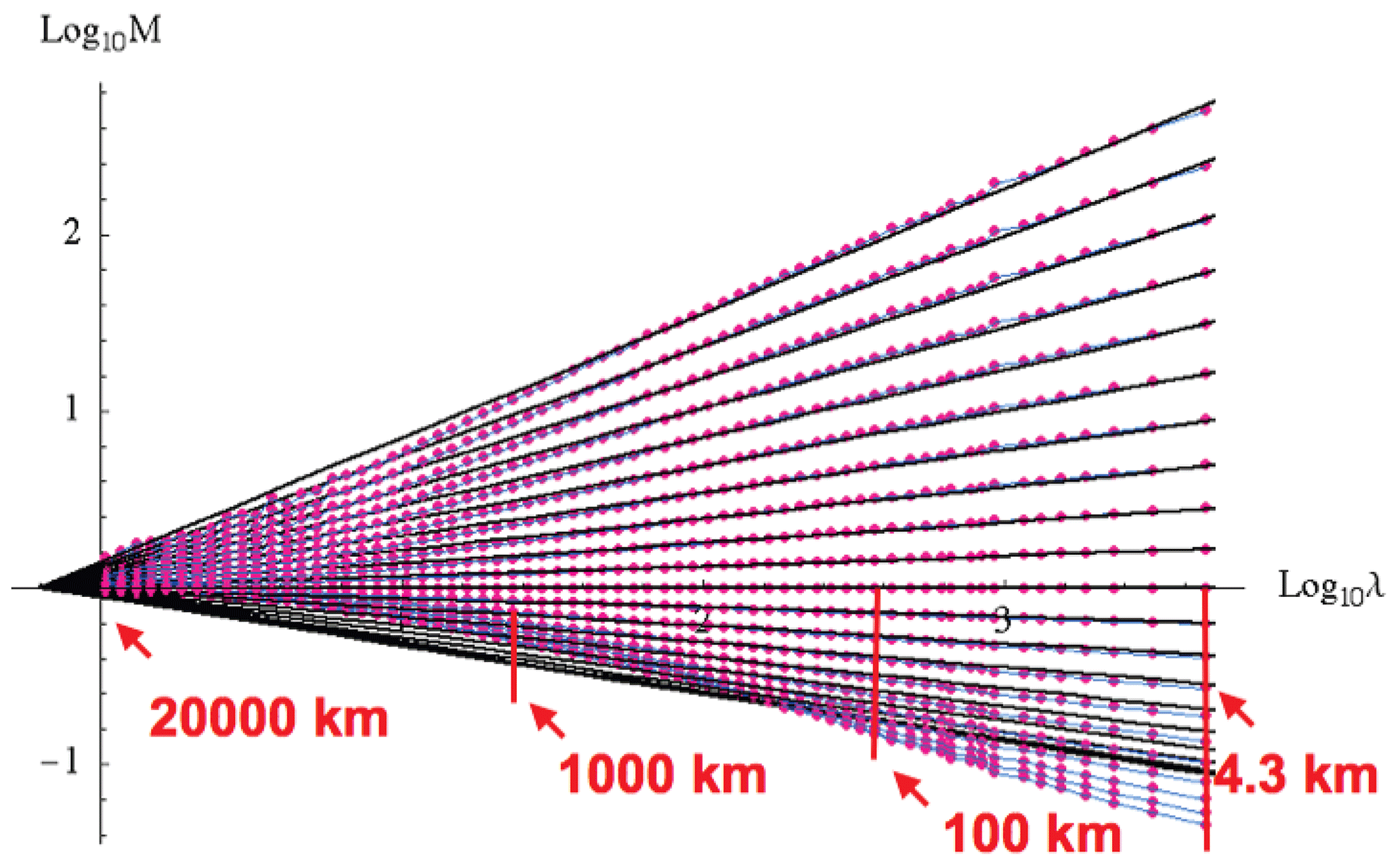
Figure 35The same as Fig. 34 except for TRMM reflectivities (4.3 km resolution). The moments are for , taken along the satellite track. The poor scaling (curvature) for the low q values (bottom) can be explained as artefacts of the fairly high minimum detectable signal. The reference scale used as a first estimate of the outer-cascade scale was Lref=20 000 km, and the outer scale (where the lines cross) was 32 000 km (as in Fig. 34) (Lovejoy et al., 2009e).
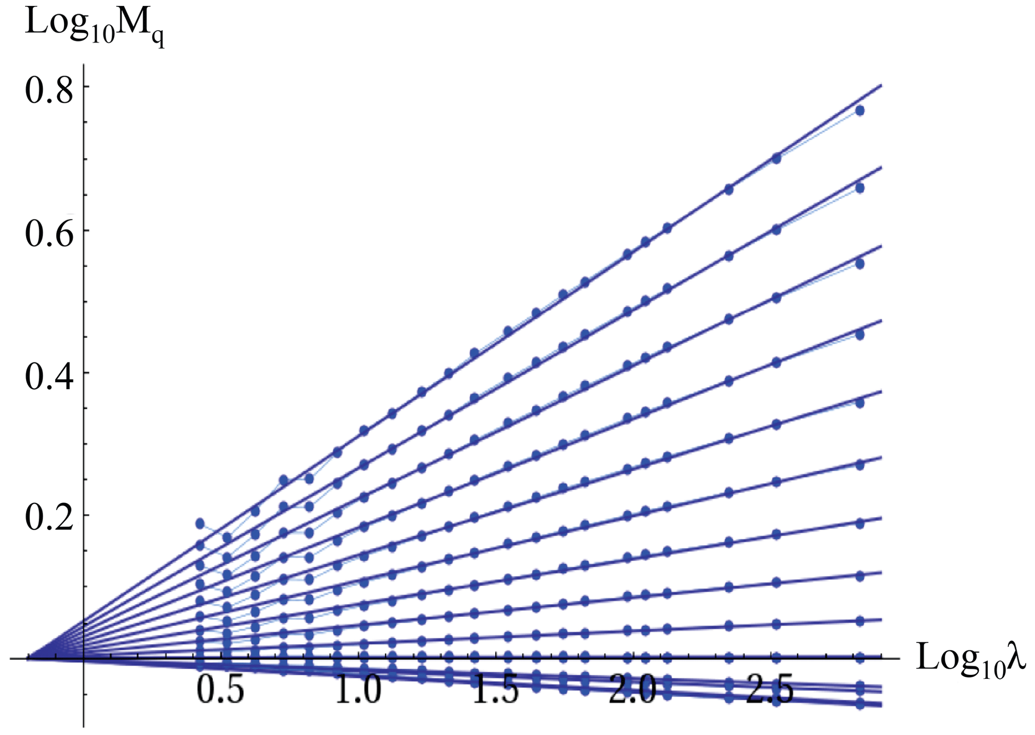
Figure 36Trace moments from (for ) for the 1440 hourly geostationary MTSAT data at a 30 km resolution, over the region 40∘ N to 30∘ S covering 130∘ of longitude over the Pacific Ocean. Lref=20 000 km, and the lines cross at an outer scale of 32 000 km. For the space–time spectra, see Fig. 25. Reproduced from Pinel et al. (2014).
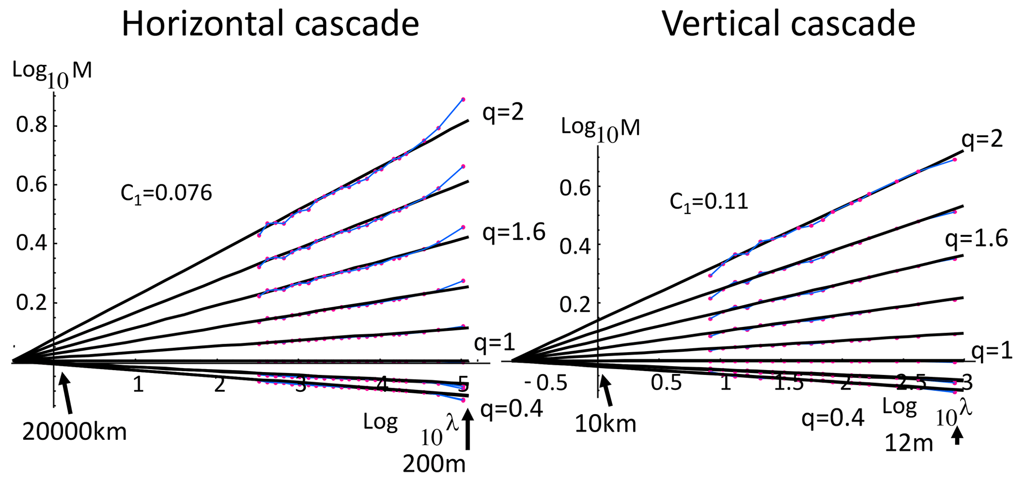
Figure 37The cascade structure of lidar aerosol backscatter; see the example in Fig. 45. Moments of normalized fluxes (indicated as M). We show the moments of order . Note how the lines converge at effective outer scales that are close to the half-circumference (left) and tropopause height (right). Also, the ratio of the intermittency parameters C1 is ≈ 0.70 ± 0.15, compatible with the theoretical ratio Hz. Reproduced from Lovejoy et al. (2009a).
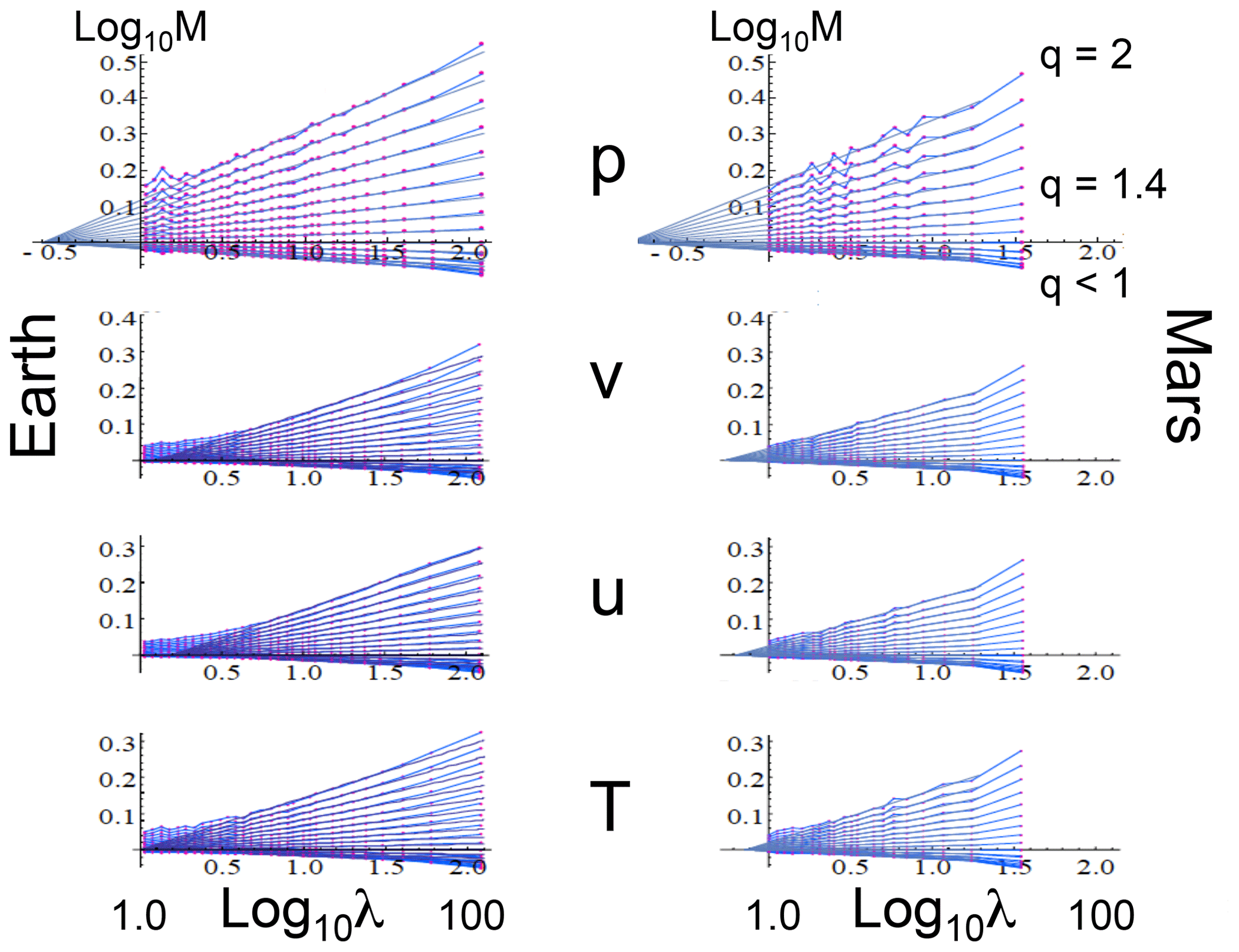
Figure 38A comparison of the scaling of the normalized fluxes (Mq(λ)) as functions of the scale ratio for both Earth (left) and Mars (right) and for surface pressure anomalies (p, top), north–south wind (v), east–west wind (u), and temperature (T, bottom). These were estimated from the fluctuations by using Eq. (18): Lref is the half-circumference of each planet, so that the scale ratio λ (denoted λref in the text) is the inverse of a nondimensional distance. For each individual plot (trace moments), the moments of order are shown as indicated (upper right). For the Earth the data were at 1∘ resolution from daily data from the ECMWF-Interim reanalysis for the year 2006, whereas for Mars, it was from the MACDA (Mars Analysis Correction Data Assimilation) reanalysis at 3.75∘ resolution over 3 Martian years (roughly 8 terrestrial years). The regression lines are fits to Eq. (14); the slopes are the exponents K(q) and the point of convergence is at the outer scale ratio: it indicates the scale at which the variability starts to build up. In all cases, it is nearly the size of the planet (λ=1). Adapted from Chen et al. (2016).
3.5 Bare and dressed multifractals and multifractal extremes
3.5.1 Power-law tails, divergence of high-order moments, and multifractal phase transitions
The multifractal process φλ in Fig. 27 is shown at various resolutions generated from data at 280 m resolution that were then systemically degraded. How could we model such a process? Let us first consider a multiplicative cascade process by starting at the bottom and (multiplicatively) adding details as we move to the top. To go from one level (resolution) to the next (i.e. λ→4λ in this example), we would use the same rule: pick four random multipliers from a unique probability distribution. In order to prevent the mean from tending to either zero or infinity, these multipliers should be normalized so that their mean is constant. At each step, the spikes would become generally sharper, depending only on the lower-resolution spikes. At each level (λ), the statistics would be characterized by the same K(q) (moments) or c(γ) (probability); this is a multifractal cascade, the generic multifractal process.
However, we can already see a problem with this naïve construct. When we reach the top (corresponding to data at 280 m resolution), we are still far from the turbulent dissipation scale that is roughly 1 million times smaller: the top line is better modelled by continuing the cascade down to very small (dissipation) scales and then – imitating the aircraft sensor – averaging the result over 280 m. A multifractal process at scale λ can thus be produced in two ways: either by a cascade that proceeds over a finite range λ and then stops – or alternatively – one that proceeds to very small scales and then is averaged to the same scale. Using renormalization jargon, the former is a “bare” multifractal process, whereas the latter – the typical empirical multifractal – is a “dressed” process. What is the difference between the statistics of the bare and dressed resolution λ multifractal processes?
Mathematically, we can represent the dressed process as
The “flux” ΠΛ(Bλ) and “volume” vol(Bλ) are D-dimensional measures over a λ resolution “ball” Bλ. In the D=1 dimensional process considered here, it is an interval (length λ−1) for isotropic processes in D=2 or and it is a square or cube (areas λ−2 and volumes λ−3 respectively, for anisotropic scaling and balls; see Sect. 4). The “λ resolution dressed” process φ(d),λ is thus the small-scale cascade limit (Λ→∞) of the λ scale average.
A basic result going back to Mandelbrot (1974) and generalized in Schertzer and Lovejoy (1985c, 1987, 1992, 1994) shows that the statistical moments are related as
i.e. the dressed moments greater than a critical order qD diverge, but below this, the bare and dressed moments are nearly the same. In terms of the moment-scaling exponents,
(“d” for “dressed”).
The critical moment for divergence qD is the solution of the implicit equation:
i.e. the qth moment converges if , where D is the dimension of space over which the averaging is performed.
We can now briefly consider the conditions under which there are nontrivial solutions to Eq. (28) with finite qD. First, note that qD>1 since otherwise the process cannot be normalized. Then recall that K(q) is convex () and K(1)=0 (the mean is independent of scale: it is “conserved”). There is therefore a trivial solution at q=1; the solution we require – if it exists – is for q>1. Such solutions qD to Eq. (28) are found at the intersection of K(q) with the line slope D passing through the axis at q=1 for q>1.
It is now convenient to define the strictly increasing “dual” codimension function C(q):
(see Fig. 39 for a graphical representation of this relationship). The equation for divergence is now C(qD)=D and the condition is . Since C(1)<D and C(q) increase with q, then, whenever C(∞)>D, there will be a nontrivial qD. For universal multifractals, this is always the case when the Lévy index α≥1.
To find the corresponding dressed probability exponent cd(γ), we can now take the Legendre transform (Eq. 22) of Kd(q):
where γD is the singularity corresponding to the critical moment qD: . Finally, with this dressed cd(γ), we easily find that the tails of the probability distributions are power laws:
Such tails are sometimes called “fat” or “Pareto”. Note that, unlike additive processes (e.g. sums of random variables) that generally give rise to stable Lévy distributions with divergence order restricted to exponents qD<2, in these multiplicative cascade processes, qD can have any value >1. Finally, since the exponent functions K(q) and c(γ) have thermodynamic analogues, the discontinuities in the dressed quantities can be theorized as “multifractal phase transitions” of various orders (Schertzer and Lovejoy, 1992). Finally, since no empirical value is infinite – infinite moments occur only in the limit of averages over an infinite number of realizations – the moments q>qD will be finite but spurious: see the full theory in Schertzer and Lovejoy (1992), summarized in Chap. 5 of Lovejoy and Schertzer (2013).
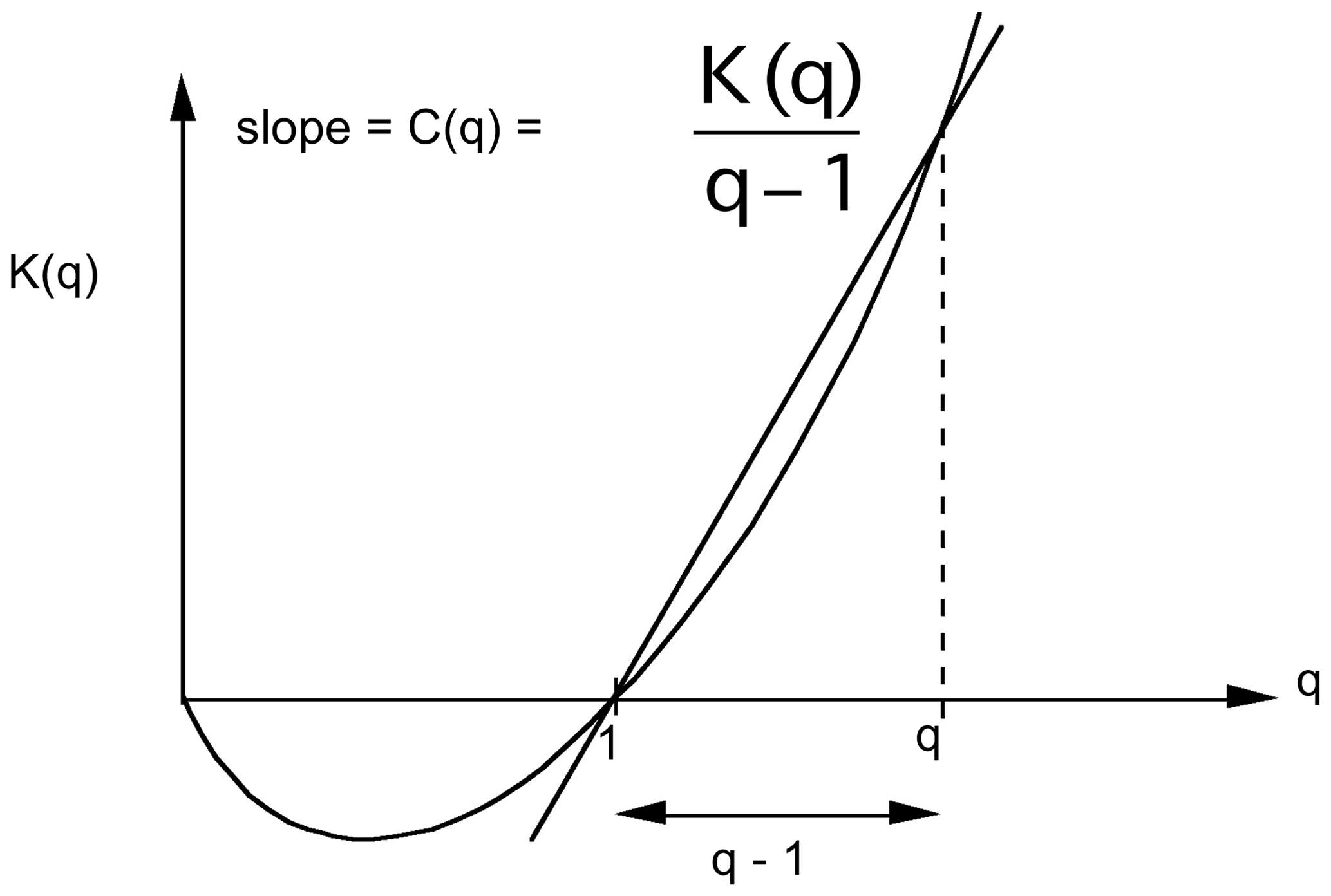
Figure 39A schematic illustration of the relation between K(q) and C(q). Reproduced from Lovejoy and Schertzer (2013).
3.5.2 Power-law tails, outliers, black swans, and tipping points
To get an idea of how extreme the extremes can be, consider the temperature fluctuations with qD=5 (Fig. 40 and Table 2). For a Gaussian, temperature fluctuations 10 times larger than typical fluctuations would be ≈1023 times less likely; if observed, they would be classified as outliers. However, with a power-law tail and qD=5, such extremes occur only 105 times less frequently, so that, although rare, they are no longer outliers. In the context of temperatures, understanding the nature of the extremes is fundamental since it determines our interpretation of large events as either extreme – but nevertheless within the expected range and hence “normal” – or outside this range and hence an “outlier” or perhaps – notably in climate applications – even a “tipping point”.
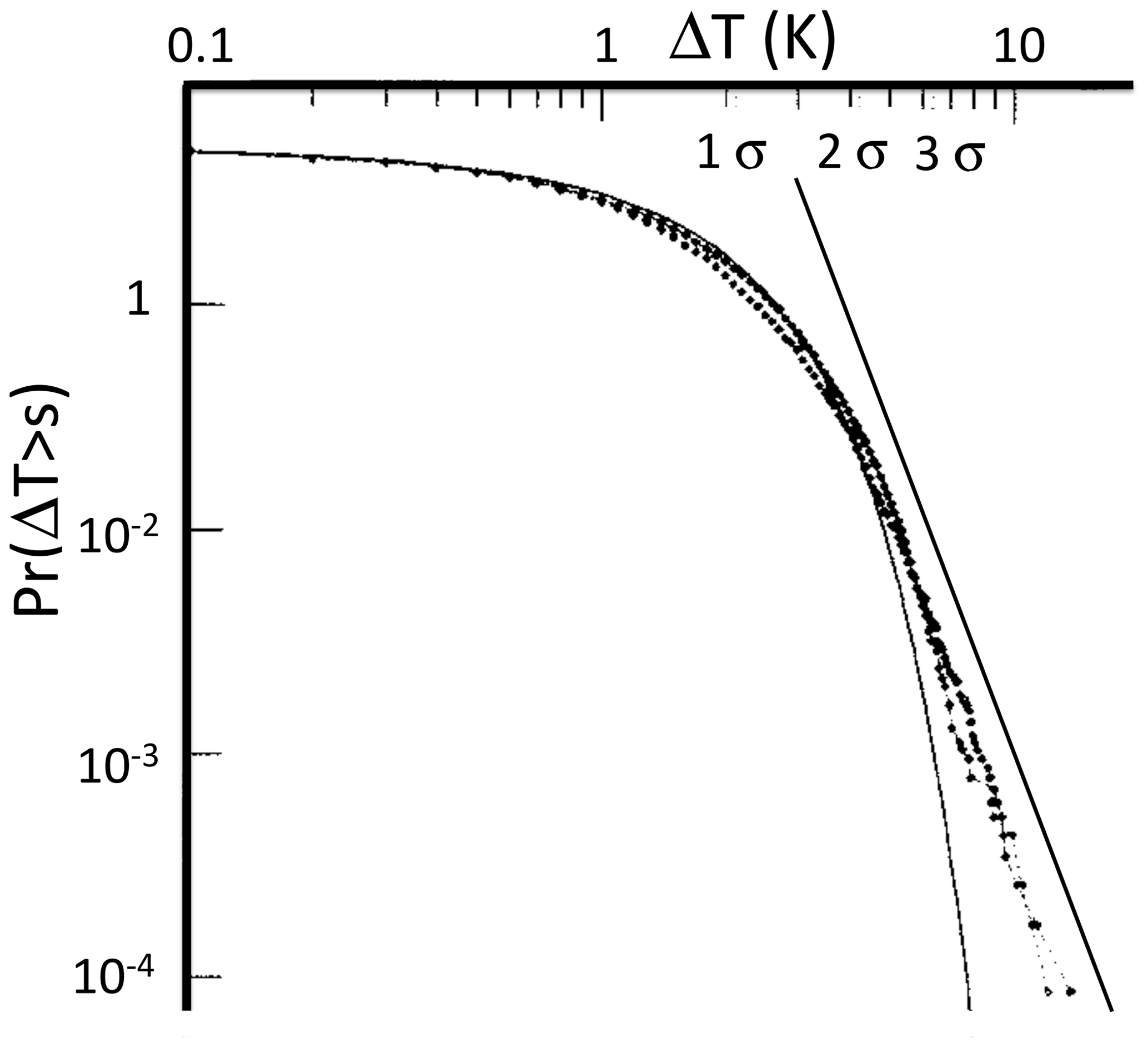
Figure 40The probability distribution of daily temperature differences in daily mean temperatures from Macon, France, for the period 1949–1979 (10 957 d). Positive and negative differences are shown as separate curves. A best-fit Gaussian is shown for reference, indicating that the extreme fluctuations correspond to more than 7 standard deviations. For a Gaussian this has a probability of 10−20. The straight reference line (added) has an absolute slope of qD with qD=5. Adapted from Ladoy et al. (1991).
A relevant example of the importance of the power-law extremes is global warming. Over about a century, there has been 1 ∘C warming of the globally averaged temperature – an event of roughly 5 standard deviations (with Gaussian probability ≈ 3 × 10⁻⁶). In spite of this, climate skeptics claim that it is no more than a giant natural fluctuation (GNF), i.e. a change that might nevertheless be normal – albeit extreme. The relevant extreme centennial changes are indeed non-Gaussian, and bounding the probability tail between power laws with , Lovejoy (2014) showed that the probability of extremes was enhanced by a factor of as much as 1000. However, the GNF hypothesis could nevertheless be statistically rejected with more than 99.9 % confidence.
There are now numerous atmospheric fields whose extremes have been studied and power-tail exponents (qD) estimated. Some of these are shown in Table 2 (reproduced from Lovejoy and Schertzer, 2013), and the wind field is discussed in the next section.
Table 2A summary of various estimates of the critical order of divergence of moments (qD) for various meteorological fields (reproduced from Lovejoy and Schertzer, 2013). The numerous estimates of qD in precipitation are not included; they are more fully reviewed in Lovejoy and Schertzer (2013), and typical estimates are qD≈3.
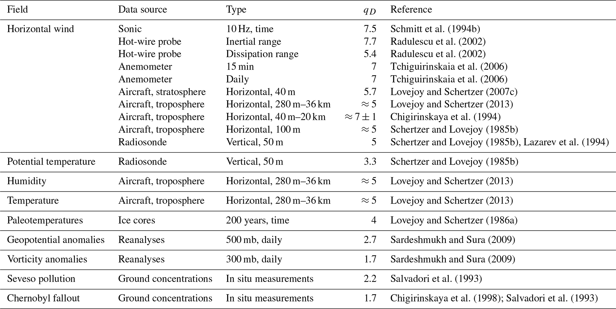
3.5.3 The divergence of high-order velocity moments
While the temperature is of fundamental significance for the climate, the wind is the dynamical field, so that it is analogously important at weather scales (as well as in mechanically forced turbulence). For example, numerous statistical models of fully developed turbulence are based on “closure” assumptions that relate high-order statistical moments to lower-order ones, thus allowing the evolution of the statistics in high Reynolds number turbulence to be modelled. Closures thus postulate the finiteness of some (usually all) high-order statistical moments of the velocity field.
In fully developed turbulence, in the inertial (scaling) range, ε is conserved by the nonlinear terms in the Navier–Stokes equations; this is the basis of the Kolmogorov law and of cascade theories. In this range, the Kolmogorov law gives ε∝Δv3. However, at small enough (dissipation) scales, where the dynamics are dominated by viscosity, dimensional analysis shows that ε∝Δv2. For the probability exponents, these relations imply that (inertial range) and (dissipation range). Since ε is expected to be constant throughout the inertial range – and in the dissipation range to be equal to the dissipation – we expect ; hence, the ratio of velocity exponents in the two ranges is .
Before discussing this further, let us consider the evidence for the divergence of high-order moments in the velocity/wind field. The earliest evidence is shown in Fig. 41 (left): it comes from radiosondes (balloons) measuring the changes in horizontal wind velocity in the vertical direction. Schertzer and Lovejoy (1985c) found as shown in the plot that extends over layers of thicknesses varying from 50 to 3200 m. In Fig. 41 (from the same paper), probability distributions of ε are shown from aircraft data, with ; we see that these exponents approximately satisfy the above inertial range theory: .
These early results had only order 102–103 measurements, which only allows the determination of probabilities down to levels of 10−2–10−3; this is barely enough to robustly characterize the exponents. More recent aircraft results with nearly the same horizontal exponent () were obtained from another aircraft data set, this time with ≈ 106 data points (Fig. 42, right, Lovejoy and Schertzer, 2007b). A probability distribution in the time domain also with ≈ 106 points is shown in Fig. 42 (left); it was obtained using a sonic anemometer at 10 Hz (Schmitt et al., 1994b). Here, the exponent is .5, i.e. a bit larger than in space.
Results from a much larger sample and from a more controlled laboratory setting (a wind tunnel), also in the temporal domain, are shown in Fig. 43 (data taken from Mydlarski and Warhaft, 1998, and analysed in Radulescu et al., 2002, and Lovejoy and Schertzer, 2013). In this case, by placing sensors at varying separations, one can estimate the exponents in both the inertial and dissipation ranges. In the inertial range, the result () is very close to the earlier temporal result (Fig. 43, left: the truncation at large Δv is explained by experimental limitations; Lovejoy and Schertzer, 2013), whereas in the dissipation range, it has the lower value . The ratio .43 is very close to the theoretical ratio noted above with the value qD,ε ≈ 2.7. This good verification of the theoretical result lends credence to the theory and to the reality of the divergence itself.
The previous results from the wind and laboratory turbulence allowed estimates of the probability tails down to levels of only about 10−6. A more recent result (Fig. 44) is about 1 billion times larger. This is from the largest direct numerical simulation (DNS) to date, using (213)3 discrete-volume elements. This high Reynolds number incompressible Navier–Stokes turbulence (Yeung et al., 2015) allows us to reach much lower probability levels (p≈ 10−15). Figure 43 shows that, over ≈ 6 orders of magnitude, the probability tails of ε (and of enstrophy) have . Surprisingly, although the plot was made explicitly to reveal the nature of extreme fluctuations and the theory predicting the divergence of moments in turbulence (Mandelbrot, 1974; Schertzer and Lovejoy, 1987, Eqs. 26 and 30), this striking power-law behaviour of the extremes was not even mentioned by Yeung et al. (2015); it was apparently only first noted in Lovejoy (2019).
We could note that values imply the divergence of the second moment (i.e. the variance) of ε. This divergence is theoretically significant since – following Kolmogorov (1962), who proposed a log-normal distribution of ε (i.e. with all moments finite) – the variance of ε is regularly used to characterize turbulent intermittency, but we now see that, due to the divergence, this characterization is problematic. In practice, no empirical result is ever infinite. What diverging moments imply is rather that, when one attempts to empirically estimate them, the estimates get larger and larger as the sample size increases. Different experiments can thus readily get quite different results, and the parameters are not at all robust.
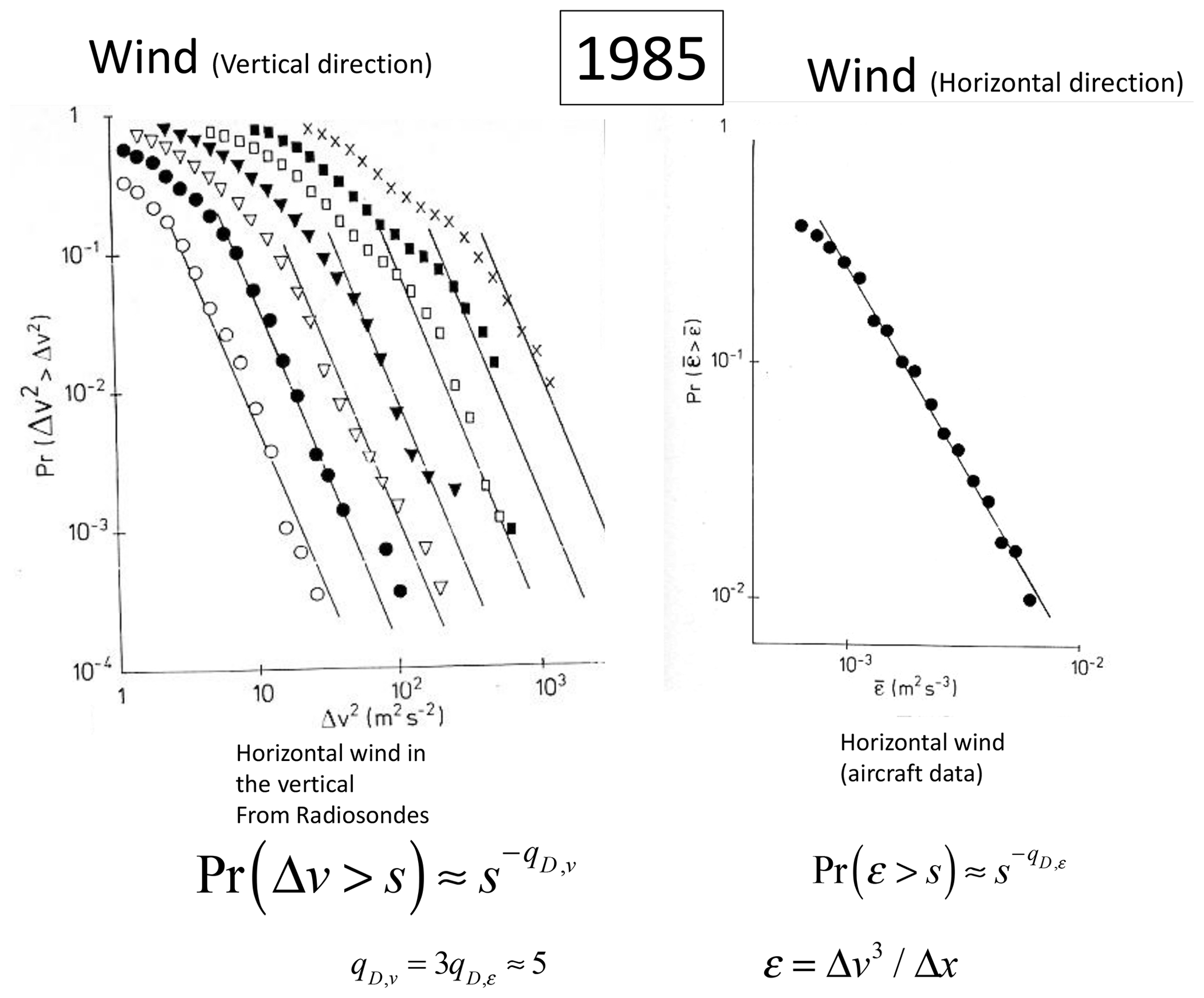
Figure 41The left-hand-side plot shows the probability distribution of the squares of horizontal wind differences in the vertical direction, estimated from radiosondes. The curves from left to right are for layer thicknesses 50, 100, … 3200 m. The curves' straight reference lines have slopes corresponding to qD=5. The separation of each curve is 2Hv with , the Bolgiano–Obukhov value; see Sect. 4. The plot on the right is for the probability distribution of ε estimated in the horizontal from aircraft spectra. The straight line has slope ; since ε∝Δv3, this corresponds to qD=5 for the wind. Both figures are adapted from Schertzer and Lovejoy (1985c).
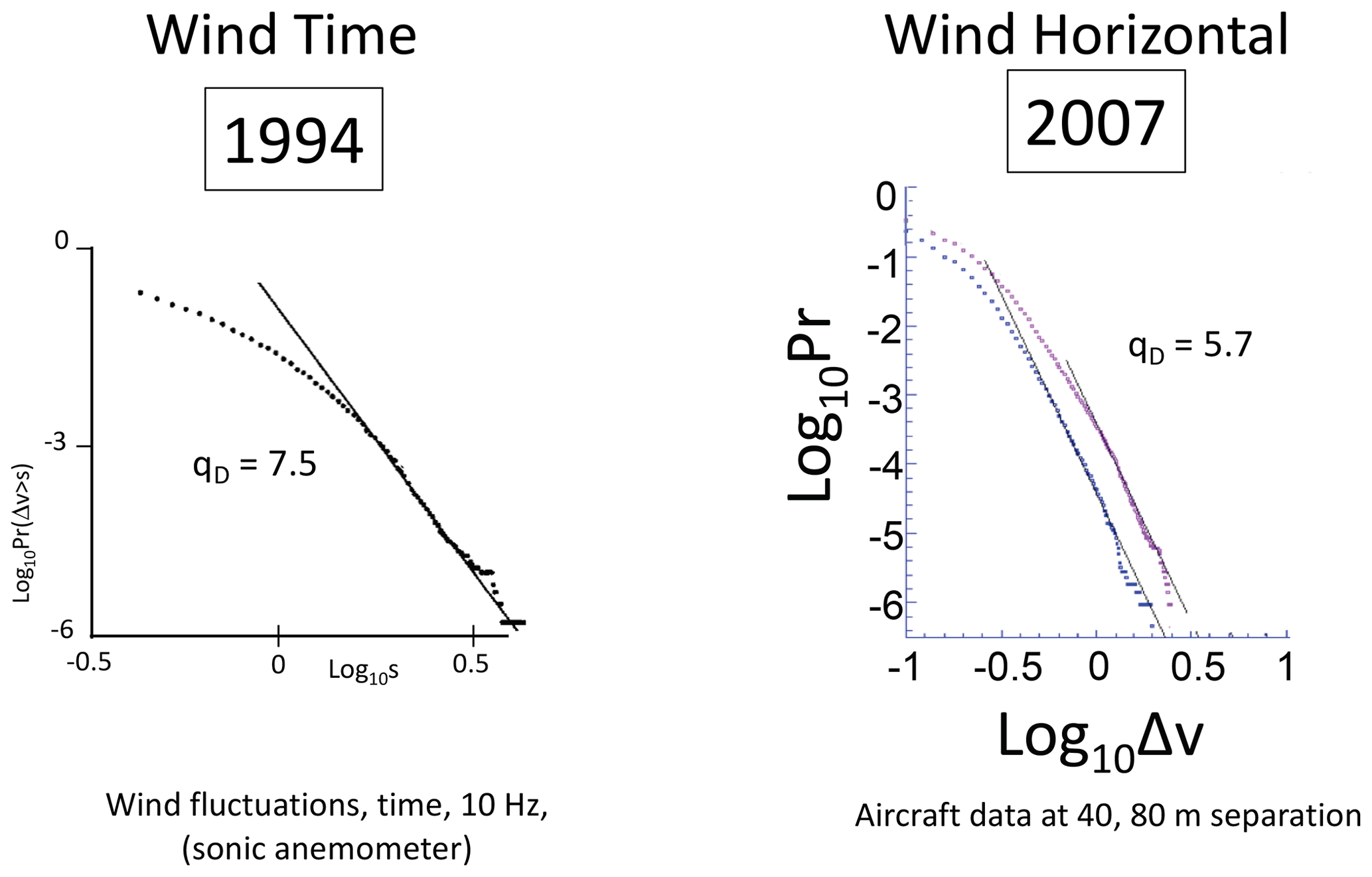
Figure 42The left-hand-side figure shows the probability distribution of changes Δv in the horizontal wind as measured by a sonic anemometer at 10 Hz. The reference slope corresponds to qD=7.5 (adapted from Schmitt et al., 1994a). The figure on the right shows the differences in horizontal wind from 24 aircraft trajectories flying near 12 km altitude; results are shown for separations of 40 and 80 m, and reference slopes corresponding to qD=5.7 are shown. Adapted from Lovejoy and Schertzer (2007b).
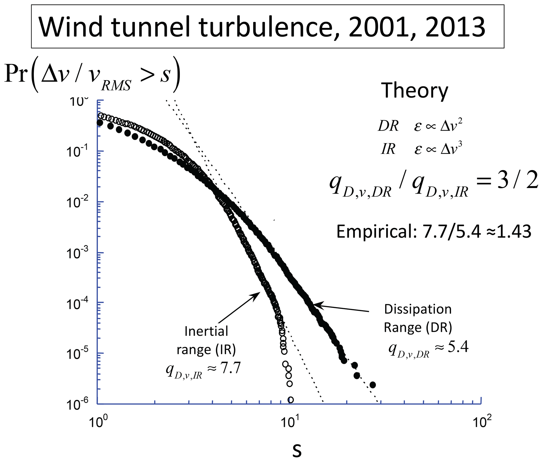
Figure 43Probability distributions from laboratory turbulence from pairs of anemometers separated by small dissipation range (DR) distances and larger (IR) distances. Slopes corresponding to qD=5.4 and 7.7 respectively are shown. Their theoretical ratio is 3 : 2, close to the empirical ratio 1.43. Reproduced from Lovejoy and Schertzer (2013).
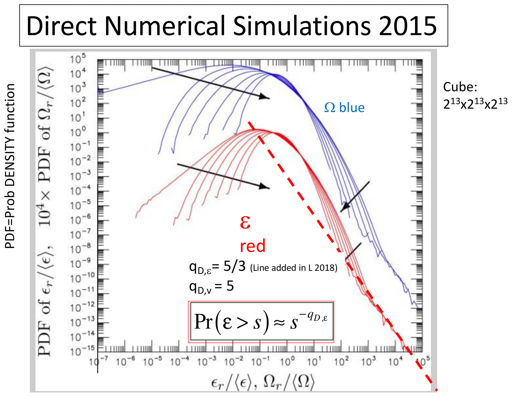
Figure 44Probability distributions of enstrophy (W) and energy (e) fluxes from a large direct numerical simulation of incompressible hydrodynamic turbulence ((213)3), adapted from Yeung et al. (2015) by adding the dashed reference line corresponding to for the velocity qD,v.
3.5.4 Power-law probabilities may be more common than we think
In these log–log plots of probability densities, we see that most of the distributions show evidence of log–log linearity near the extremes. When judging possible deviations, it could be recalled that, due to inadequate instrumental response times, postprocessing noise-reduction procedures (e.g. smoothing), or outlier-elimination algorithms, extremes can easily be underestimated. Since, physically, the extremes are consequences of variability building up over a wide range of spatial scales, we expect that numerical model outputs (including reanalyses) will underestimate the extremes. For example, Lovejoy (2018) argued that the models' small hyperviscous scale range (truncated at ≈ 105 m rather than at the viscous scale of ≈ 10−3 m) effectively truncates the extreme tails. Any of these effects may explain deviations from perfect power-law tails or might explain some of the larger (i.e. less extreme) qD values in Table 2. Finally, while power-law probabilities arise naturally in scaling systems, the distributions are not necessarily power laws; non-power laws (curved tails) may simply correspond to the special cases where qD→∞ (as with the non-intermittent Gaussian special cases).
3.5.5 The Noah effect, black swans, and tipping points
The power-law fluctuations in Figs. 41–44 are so large that, according to classical assumptions, they would be outliers. In atmospheric science, thanks to the scaling, very few processes are Gaussian and extremes occur much more frequently than expected, a fact that colleagues and I regularly underscored starting in the 1980s (see Table 2 and, for a review, Chap. 5 of Lovejoy and Schertzer, 2013).
At best, Gaussians can be justified for additive processes, with the added restriction that the variance is finite. However, once this restriction is dropped, we obtain “Lévy distributions” with power-law extremes but with exponents qD<2 (see however Ditlevsen, 1999). Mandelbrot and Wallis (1968) called the Lévy case the “Noah effect” after the Biblical Flood. The Gaussian assumption also fails for the additive but scaling H model (Lovejoy, 2015; Lovejoy and Mandelbrot, 1985). Most importantly, Gaussians are irrelevant for multiplicative processes: these generally lead to power-law extremes but without any restriction on the value of qD (Mandelbrot, 1974; Schertzer and Lovejoy, 1987). Related models include self-organized criticality (Bak et al., 1987) and correlated additive and multiplicative noise (Sardeshmukh and Sura, 2009). We could also mention that power-law distributions also appear as the special (Frechet) case of generalized extreme-value distributions, although, due to long-range statistical dependencies, standard extreme-value theory does not generally apply to scaling processes.
To underscore the importance of nonclassical extremes, Taleb introduced the terms “grey and black swans” (Taleb, 2010). Originally, the former designated Lévy extremes, and the latter was reserved for extremes that were so strong that they were outliers with respect to any existing theory. However, the term “grey swan” never stuck, and the better-known expression “black swan” is increasingly used for any power-law extremes.
All of this is important in climate science, where extreme events are often associated with tipping points. The existence of black swan extremes leads to a conundrum: since black swans already lead to exceptionally big extremes, how can we distinguish “mere” black swans from true tipping points?
4.1 Generalized scale invariance
4.1.1 Discussion
So far, we have only discussed scaling in 1D (series and transects), so that the notion of scale itself can be taken simply as an interval (space) or lag (time), and large scales are simply obtained from small ones by multiplying by their scale ratio λ. However, series and transects are only 1D subspaces of the full space–time where atmospheric processes are defined. In order to answer the question “how big is a cloud?” – i.e. for more general atmospheric applications – we need to define the scale in 3D space and, for its evolution, in 4D space and time.
The most obvious problem is stratification in the horizontal (see Figs. 4 and 5). This is graphically shown in Fig. 45 of airborne lidar backscatter from aerosols. At low resolution (bottom), one can see highly stratified layers. However, zooming in (top) shows that the layers have small structures that are in fact quite “roundish” and hinting that, at even higher resolutions, there might be stratification instead in the vertical. If we determine the spectra in the horizontal and compare them with those in the vertical, we obtain Fig. 46; the spectra show power laws in both directions but with markedly different exponents. As shown below, it turns out that the key ratio is
where h indicates horizontal and v vertical (see Eq. 9), with the value predicted by the 23/9D model (discussed below). In the figure we see that this prediction is well satisfied by the data. If the atmosphere is scaling but stratified, then the transects and series must more generally have different exponents, ξ(q), H, and K(q), but for any q, the ratio of horizontal to vertical exponents is Hz.
The difference in horizontal and vertical exponents is a consequence of scaling stratification: the squashing of structures with scale. In the simplest case, called “self-affinity”, the squashing is along orthogonal directions that are the same everywhere in space – for example along the y axis in an x−y space. More generally, there is also rotation of structures with scale, and the anisotropy depends not only on scale, but also on position. We need more general nonclassical (non-Euclidean) notions of scale and scale change: this is GSI (Schertzer and Lovejoy, 1985a; for a review, see Chap. 7 of Lovejoy and Schertzer, 2013, or for a nontechnical overview, see Chap. 3 of Lovejoy, 2019). Note that the following presentation is based on scale functions, and these can be used to define anisotropic Hausdorff measures, hence providing a (mathematical) measure-based definition of size (Schertzer and Lovejoy, 1985a).
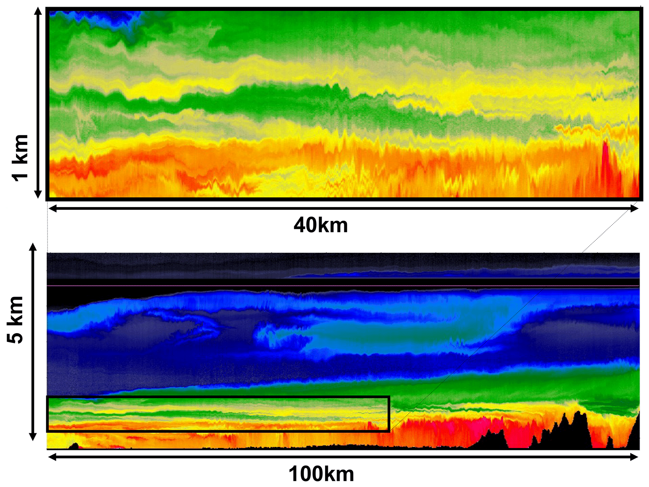
Figure 45Bottom: a vertical section of laser backscatter from aerosols (smog particles) taken by an airborne lidar (laser) flying at 4.5 km altitude (purple line) over British Columbia near Vancouver (the topography is shown in black; the lidar shoots two beams, one up and one down) (Lilley et al., 2004). The resolution is 3 m in the vertical and 96 m in the horizontal. The top panel is at a fairly coarse resolution, and we mostly see a layered structure. Top: the black box in the lower left is shown blown up at the top of the figure. We are now starting to discern vertically aligned and roundish structures. The aspect ratio is about 40:1, reproduced from Lilley et al. (2004).
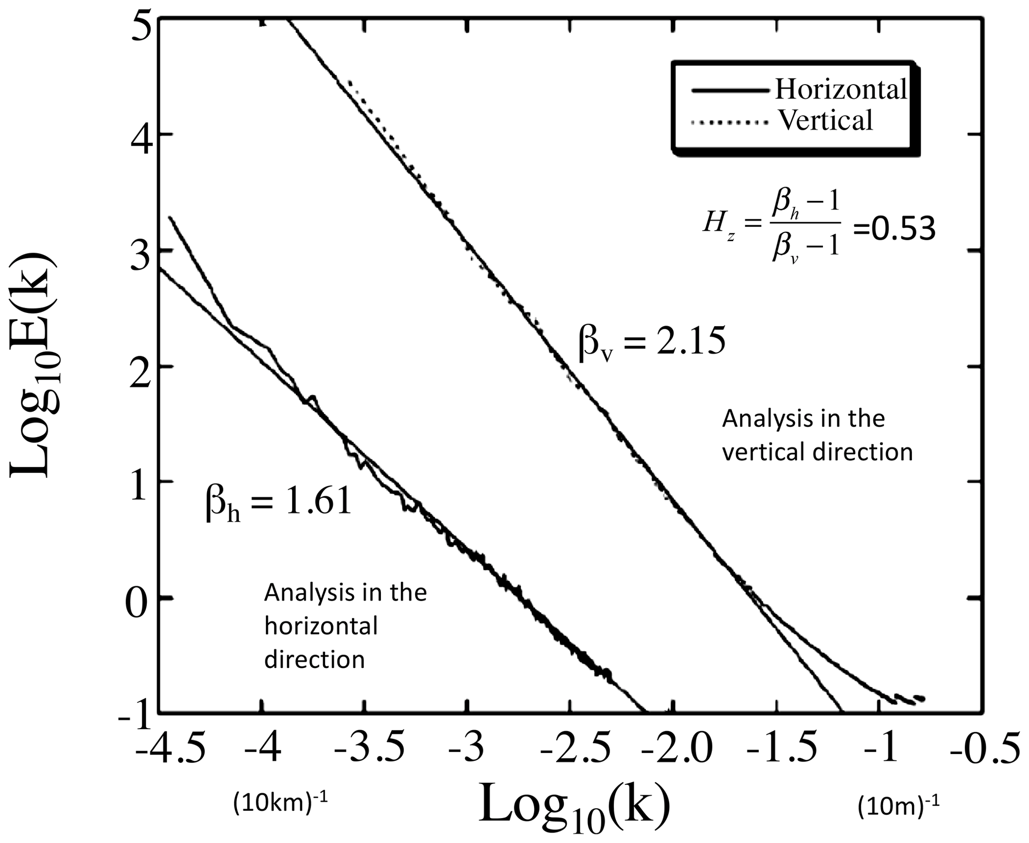
Figure 46The lower curve is the power spectrum for the fluctuations in the lidar backscatter ratio, a surrogate for the aerosol density (B) as a function of horizontal wavenumber k (m−1) with a line of best fit with slope βh=1.61. The upper trace is the power spectrum for the fluctuations in B as a function of vertical number k with a line of best fit with slope βv=2.15. Adapted from Lilley et al. (2004).
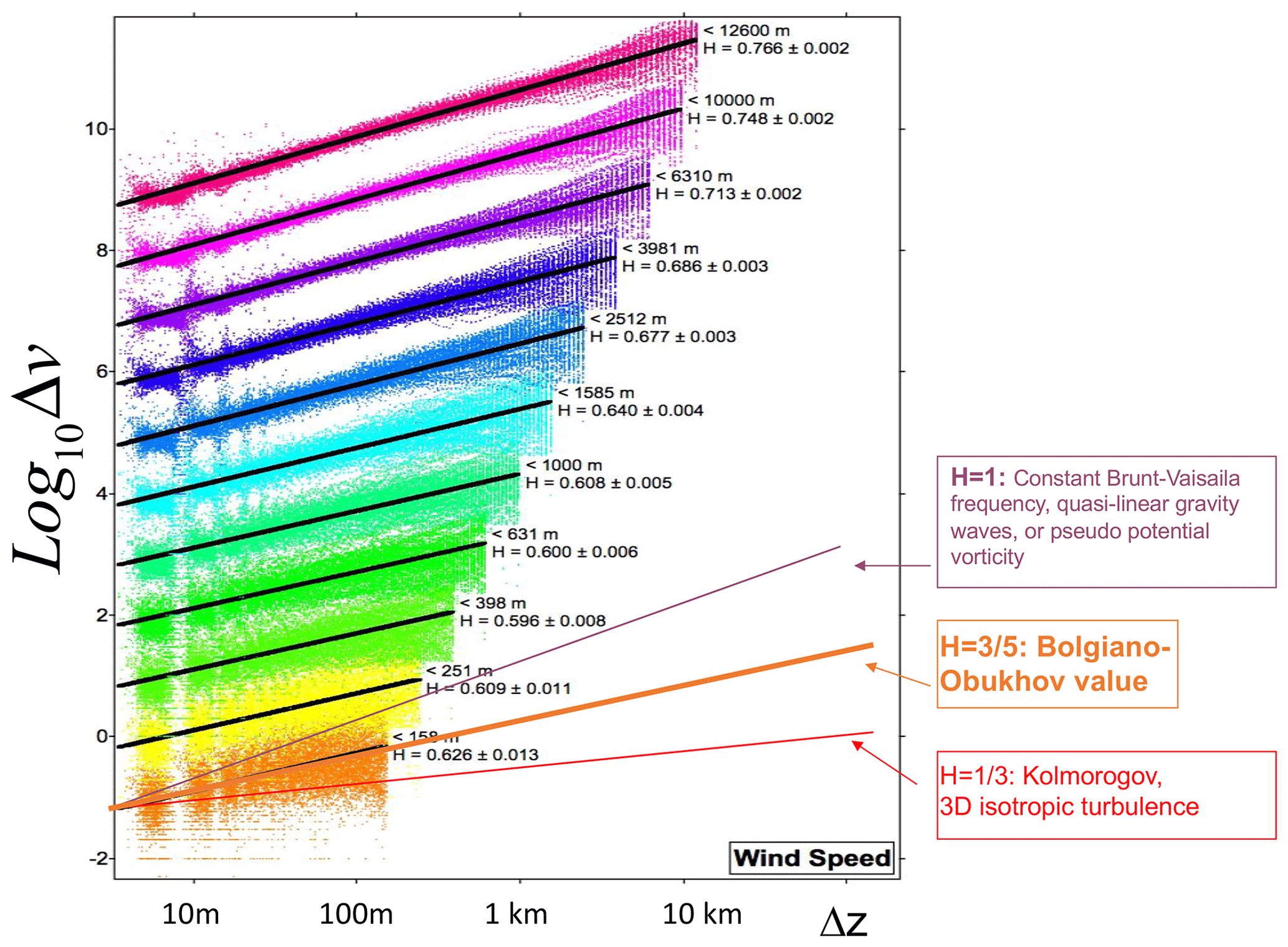
Figure 47The average mean absolute difference in the horizontal wind from 238 dropsondes over the Pacific Ocean taken in 2004. The data were analysed over regions from the surface to higher and higher altitudes (the different lines from bottom to top, separated by a factor of 10 for clarity). Layers of thickness Δz increasing from 5 m to the thicknesses spanning the region were estimated and lines fitted corresponding to power laws with the exponents as indicated. At the bottom, reference lines with slopes (Kolmogorov, K), (Bolgiano–Obukhov, BO), and 1 (gravity waves, GWs, and quasi-geostrophic turbulence) are shown for reference. Reproduced from Lovejoy et al. (2007), and see Hovde et al. (2011).
4.1.2 Scale functions and scale-changing operators: from self-similarity to self-affinity
To deal with anisotropic scaling, we need an anisotropic definition of the notion of scale itself.
The simplest scaling stratification is called self-affinity: the squashing is along orthogonal directions whose directions are the same everywhere in space – for example along the x and z axes in an x−z space, e.g. a vertical section of the atmosphere or solid Earth. More generally, even horizontal sections will not be self-similar: as the scale changes, structures will be both squashed and rotated with scale. A final complication is that the anisotropy can depend not only on scale, but also on position. Both cases can be dealt with by using the GSI formalism corresponding respectively to linear (scale only) and nonlinear (scale and position) GSI (Lovejoy and Schertzer, 2013, Chap. 7; Lovejoy, 2019, Chap. 3).
The problem is to define the notion of scale in a system where there is no characteristic size. Often, the simplest (but usually unrealistic) self-similar system is simply assumed without question: the notion of scale is taken to be isotropic. In this case, it is sufficient to define the scale of a vector by the usual vector norm (in a vertical section , the length of the vector denoted by ). satisfies the following elementary scaling rule:
where again λ is a scale ratio. When λ>1, this equation says that the scale (here, length) of the reduced, shrunken vector is simply reduced by the factor λ−1, a statement that holds for any orientation of .
To generalize this, we introduce a scale function as well as a more general scale-changing operator Tλ; together they satisfy the analogous equation:
For the system to be scaling, a reduction by scale ratio λ1 followed by a reduction λ2 should be equal to the first reduction by λ2 and then by λ1, and both should be equivalent to a single reduction by factor λ=λ1λ2. The scale-changing operator therefore satisfies multiplicative group properties so Tλ is a one-parameter Lie group with generator G:
when G is the identity operator (I), then , so that the scale reduction is the same in all directions (an isotropic reduction): . However, a scale function that is symmetric with respect to such isotropic changes is not necessarily equal to the usual norm since the vectors with a unit scale (i.e. those that satisfy may be any (nonconstant, hence anisotropic) function of the polar angle – they are not necessarily circles (2D) or spheres (3D). Indeed, in order to complete the scale function definition, we must specify all the vectors whose scale is unity – the “unit ball”. If, in addition to G=I, the unit scale is a circle (sphere), then the two conditions imply and we recover Eq. (33). In the more general but still linear case where G is a linear operator (a matrix), Tλ depends on scale but is independent of location. In this case, the qualitative behaviour of the scale functions depends on whether the eigenvalues of G are real or complex. In the former case there is only a finite rotation of structures with scale, and in the latter, structures rotate an infinite number of times as the scale λ goes from 1 to infinity. More generally, in nonlinear GSI G also depends on location and scale: Figs. 48 and 52–55 give some examples of scale functions and Figs. 56–66 and 69 show some of the corresponding multifractal cloud simulations. For simulations of the Earth's magnetization, rock density, gravity, and topography, see Lavallée et al. (1993), Pecknold et al. (2001), Lovejoy and Schertzer (2007a), and Lovejoy et al. (2005).
4.1.3 Scaling stratification
GSI is exploited in modelling and analysing many atmospheric fields (wind, temperature, humidity, precipitation, cloud density, aerosol concentrations; see Lovejoy and Schertzer, 2013). To give the idea, we can define the “canonical” scale function for the simplest stratified system representing a vertical (x,z) section in the atmosphere or solid Earth:
Hz characterizes the degree of stratification (see below) and ls is the “spheroscale”, so called because it defines the scale at which horizontal and vertical extents of structures are equal (although they are generally not exactly circular):
It can be seen by inspection that ∥x,z∥ satisfies
(note that matrix exponentiation is simple only for diagonal matrices – here – but when G is not diagonal, it can be calculated by expanding the series or alternatively by transforming to a diagonal frame). Note that, in this case, the ratios of the horizontal and vertical statistical exponents, i.e. ξ(q), H, K(q), and c(γ), are equal to Hz. We could also note that linear transects taken in any direction other than the horizontal or vertical will have two scaling regimes (with a break near the spheroscale). However, the break is spurious: it is a consequence of using the wrong notion of scale.
Figure 48 shows some examples of lines of constant scale function defined by Eq. (36) with varying Hz values. Successive ellipses are related by the operator Tλ with in the illustration. It can be seen that, while horizontal scales are changed by a factor λ, vertical scales are changed by , and hence cross-sectional areas are changed by
The exponent Del is called the “elliptical dimension” (although the curves of constant scale are generally only roughly elliptical). Similarly, in 3D space, if there are two horizontal directions that scale as λ−1 and the vertical scales as λ−Hz, then the elliptical dimension is . Figure 11 shows a schematic of various models of the atmosphere, with the classical 2D isotropic (totally stratified, flat) large-scale model at one extreme and the 3D isotropic model at the other and the more realistic Del= 23/9D model discussed below. Interestingly, in the atmosphere – although highly variable – ls is typically small (metres to hundreds of metres), but Hz<1 (close to the middle top set of curves in Fig. 48). In contrast, in the solid Earth, ls is very large (probably larger than the planet scale), but Hz>1 (probably ≈2, close to the bottom-right curves; see Lovejoy and Schertzer, 2007a, for a review). In the former, the stratification becomes stronger at larger and larger scales, whereas in the latter, it is stronger at smaller scales.
Equipped with a scale function, the general anisotropic generalization of the 1D scaling law (Eq. 12) may now be expressed by using the scale :
where v could be any scalar with anisotropic scaling properties; below it is a component of the horizontal wind. This shows that the full scaling model or full characterization of scaling requires the specification of the notion of scale via the scale-invariant generator G and unit ball (hence the scale function), the fluctuation exponent H, and the statistics of the generic anisotropic flux specified via K(q), c(γ) or – for universal multifractals – C1, α. In many practical cases – e.g. vertical stratification – the direction of the anisotropy is fairly obvious, but in horizontal sections, where there can easily be significant rotation of structures with scale, the empirical determination of G and the scale function is a difficult, generally unsolved problem.
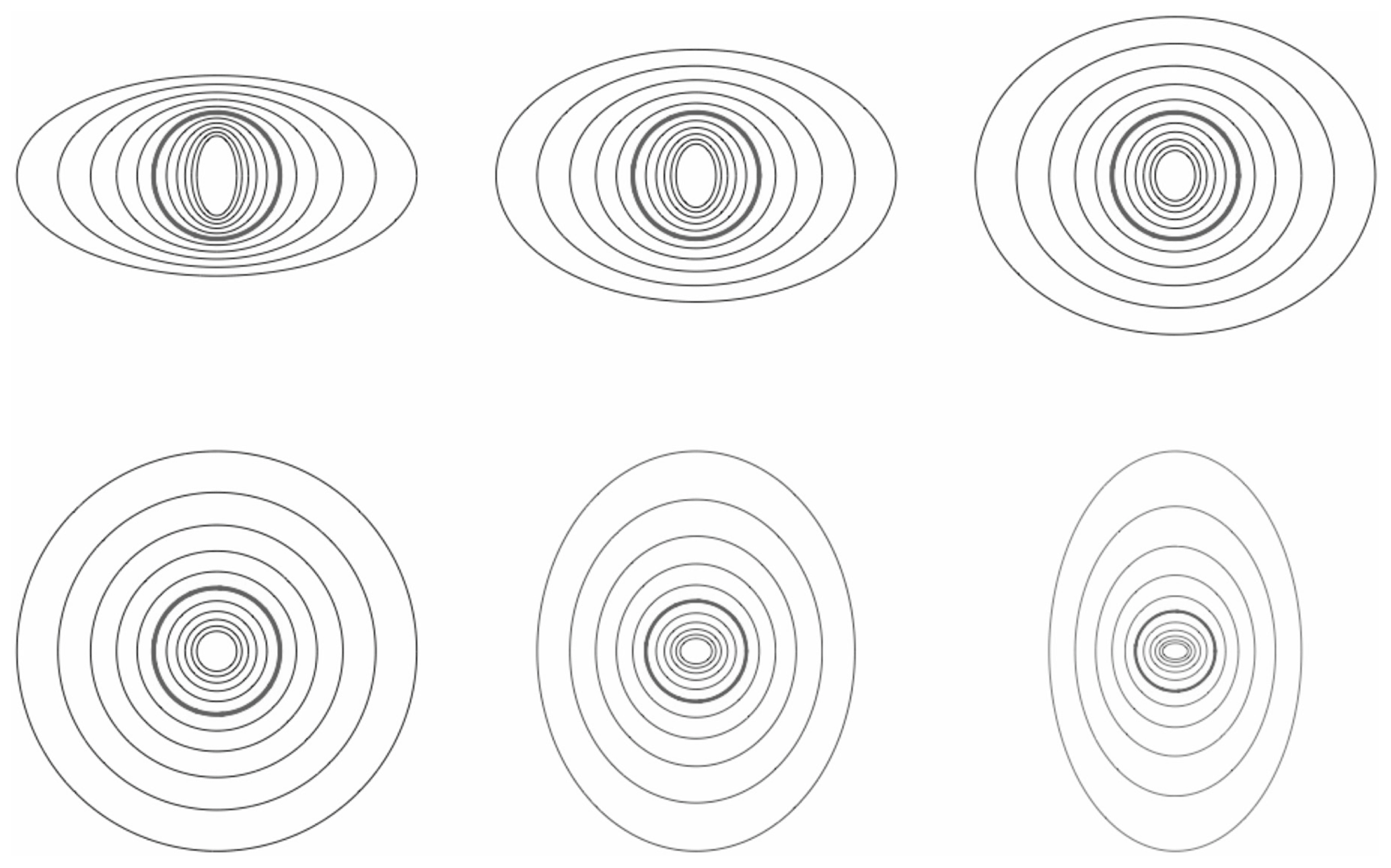
Figure 48A series of ellipses each separated by a factor of 1.26 in scale, red indicating the unit scale (here, a circle and thick lines). Upper left to lower right: Hz increasing from , , (top), 1, , (bottom, left to right). Note that, when Hz>1, the stratification on large scales is in the vertical rather than horizontal direction (this is required for modelling the Earth's geological strata). Reproduced from Lovejoy (2019).
4.1.4 The 23/9D model
Kolmogorov theory was mostly used to understand laboratory hydrodynamic turbulence, which is mechanically driven and can be made approximately isotropic (unstratified) by the use of either passive or active grids. In this case, fluctuations in Δv for points separated by can be determined essentially via dimensional analysis using ε, the latter choice being justified since it is a scale-by-scale conserved turbulent flux. The atmosphere however is fundamentally driven by solar energy fluxes which create buoyancy inhomogeneities; in addition to energy fluxes, buoyancy is also fundamental. In order to understand atmospheric dynamics, we must therefore determine which additional dimensional quantities are introduced by gravity or buoyancy. As discussed in Monin and Yaglom (1975), this is necessary for a more complete dimensional analysis.
In addition to the dynamical equations with quadratic invariant ε – the only dimensional quantity pertinent in the inertial range in isotropic turbulence – we must consider the thermodynamic energy equation for the potential temperature θ (e.g. Lesieur, 1987). Analysis shows that the v and θ fields are only coupled by the Δf buoyancy forcing term:
where g is the acceleration of gravity. f is therefore the fundamental physical and dimensional quantity rather than θ.
The classical way of dealing with buoyancy is to use the Boussinesq approximation, i.e. to assume the existence of a scale separation and then define density (and hence buoyancy) perturbations about an otherwise perfectly stratified “background” flow. This leads to the classical isotropic buoyancy subrange turbulence discovered independently by Bolgiano (1959) and Obukhov (1959). Unfortunately, it was postulated to be an isotropic range, yet it was never observed in the horizontal. Therefore, by the time it was observed later in the vertical, it had either been forgotten (Endlich et al., 1969) or its significance was not appreciated (Adelfang, 1971), and it was subsequently largely ignored.
However, if there is wide-range atmospheric scaling, then there is no scale separation (as outlined in Chap. 6 in Lovejoy and Schertzer, 2013), and so we can make a more physically based argument which is analogous to that used for deriving passive scalar variance cascades in passive scalar advection – the Corrsin–Obhukhov law (Corrsin, 1951; Obukhov, 1949) (itself analogous to the energy flux cascades that lead to the Kolmogorov law).
If we neglect dissipation and forcing, then (where is the advective derivative), so that f obeys a passive scalar advection equation and therefore the corresponding buoyancy force variance flux:
is conserved by the nonlinear terms. In this case, the only quantities available for dimensional analysis are ε (m2 s−3) and ϕ (m2 s−5). In this approach, there is no separation between a stratified “background” state and a possibly isotropic fluctuation field, so that there is no rationale for assuming that either the φ or ε cascades are associated with any isotropic regimes. Indeed, following Schertzer and Lovejoy (1983a, 1985b), it is more logical to assume that the two basic turbulent fluxes ε and ϕ can co-exist and cascade over a single-scale wide-range regime, with the former dominating in the horizontal and the latter in the vertical:
where Δx is a horizontal lag and Δz a vertical lag (for the moment we ignore the other horizontal coordinate y). Dimensionally, the fluxes ε, ϕ define a unique length scale ls:
Figure 47 shows that in the vertical the Bolgiano–Obukhov law holds quite well – especially near the surface, but at all altitudes, it is much better respected than the isotropic Kolmogorov law () or the alternative laws from quasi-linear gravity wave or quasi-geostrophic turbulence that give Hv=1 (Lovejoy et al., 2007; Hovde et al., 2011).
We can see that the two laws in Eq. (43) are special cases of the more general anisotropic scaling law Eq. (40) since, for pure horizontal displacements (Δz=0) and pure vertical displacements (Δx=0), Eq. (40) yields
If we identify and , , we see that Eqs. (40) and (45) are equivalent (use Eq. 36 for the scale functions in the horizontal and vertical directions). If, in addition, we assume that the two horizontal directions are equivalent, we obtain , hence the name “23/9D model”; see Fig. 11 for a schematic.
4.1.5 Scaling space–time, Fourier space GSI
In Sect. 2.6 and 2.7, we mentioned that for Lagrangian frame temporal velocity fluctuations we should use the size–lifetime relation that is implicit in the horizontal Kolmogorov law. If we assume horizontal isotropy, then, for velocity fluctuations, we have
Following the developments in the previous subsection (Eqs. 40 and 43), we can express the full space–time scaling (Eq. 46) in a single expression valid for any space–time vector displacement by introducing a scalar function of space–time vectors called the “(space–time) scale function”, denoted , which satisfies the fundamental (functional) scale equation:
where Gs is the 3×3 matrix spatial generator:
with rows corresponding to (), and the 4×4 matrix Gst is the extension to space and time. We have introduced the notation “[]” for the spacescale and timescale function in order to distinguish it from the purely spatial-scale function denoted “∥∥”.
Using the spacescale and timescale function, we may now write the space–time generalization of the Kolmogorov law as
where the subscripts on the flux indicate the space scale and timescale over which ε is averaged. This anisotropic intermittent (multifractal) generalization of the Kolmogorov law is thus one of the key emergent laws of atmospheric dynamics and serves as a prototype for the emergent laws governing the other fields.
The result analogous to that of the previous subsection, the corresponding simple (“canonical”) spacescale and timescale function, is
where is the “sphero-time” analogous to the spheroscale (see also Marsan et al., 1996). With the scale function (Eq. 50), the fluctuations (Eq. 49) respect Eq. (46).
We now seek to express the generalized Kolmogorov law in an Eulerian framework. The first step is to consider the effects on the scale function of an overall advection. We then consider statistical averaging over turbulent advection velocities.
Advection can be taken into account using the Galilean transformation , t→t, which corresponds to the following matrix A:
where the mean wind vector has components (Schertzer et al., 1997b) and the columns and row correspond to . The new “advected” generator is and the scale function , which is symmetric with respect to Gst,advec, is . The canonical advected scale function is therefore
Note that, since , such constant advection does not affect the elliptical dimension (“Tr” indicates “trace”; see however below for the “effective” Geff, Deff).
It will be useful to study the statistics in Fourier space; for this purpose we can use the result (e.g. Chap. 6 of Lovejoy and Schertzer, 2013) of the Fourier generator , so that
The corresponding canonical dimensional Fourier spacescale function is therefore
In other words, the real-space Galilean transformation corresponds to the Fourier space transformation (this is a well-known result, notably used in atmospheric waves).
The above results are for a deterministic advection velocity, whereas in reality, the advection is turbulent. Even if we consider a flow with zero imposed mean horizontal velocity (as argued by Tennekes, 1975) in a scaling turbulent regime with the typical largest eddy, the “weather scale” Lw will be the scale of the Earth (≈Le), will have a mean velocity , and will survive for the corresponding eddy turn over time estimated as ≈ 10 d above. In other words, if there is no break in the scaling, then we expect that smaller structures will be advected by the largest structures in the scaling regime.
The statistics of the intensity gradients of real fields are influenced by random turbulent velocity fields and involve powers of such scale functions but with appropriate “average” velocities. In this case, considering only the horizontal and time, we introduce the nondimensional variables (denoted by a circumflex “”):
The symbols μx and μy are used for the components of the nondimensional velocity; they are less cumbersome than , , where
Note that here Vw is a large-scale turbulent velocity, whereas , are given by the overall mean advection in the region of interest and μx<1, μy<1 (since ). The use of the averages (indicated by the overbars) is only totally justified if the second power of the scale function is averaged; presumably, it is some other power that is physically more relevant, and there will thus be (presumably small) intermittency corrections (which we ignore). It is now convenient to define
which satisfies . In terms of the nondimensional quantities this yields an “effective” nondimensional scale function:
where the matrix C is given in Eq. (11), its rows and columns corresponding to (left to right, top to bottom; the vertical bars indicate the usual isotropic vector norm). The effective scale function in Eq. (58) is only “trivially anisotropic” since it is scaling with respect to an “effective” G matrix the identity, the matrix C simply determining the trivial space–time anisotropy.
As discussed in Lovejoy and Schertzer (2013), the above real spacescale function is needed to interpret “satellite winds” (deduced from time series of satellite cloud images), and in Sect. 2.7 the Fourier equivalent of Eq. (58) (based on the inverse matrix C−1 and the Fourier scale function ; see Fig. 25 and Eq. 11). It was extensively empirically tested in Pinel et al. (2014), where the full parameters of the C matrix were estimated.
4.2 Empirical testing of the 23/9D model
4.2.1 Testing the 23/9D model with aircraft wind data
The first experimental measurement of the joint (Δx, Δz) structure function of the horizontal velocity was made possible by the development of aircraft navigation systems with a highly accurate TAMDAR (Tropospheric Airborne Meteorological Data Reporting) GPS-based vertical positioning system (Pinel et al., 2012, Fig. 49). High vertical accuracy is needed to distinguish aircraft flying on isobars from those flying on isoheights. The problem with earlier aircraft velocity spectra – going back to the famous and still cited (Nastrom and Gage, 1983) analysis – is that the aircraft fly on isobars, and these were gently sloping. As pointed out in Lovejoy et al. (2009c), at some critical horizontal distance (that depended on the various fluxes ε, φ, and the slope of the isobar), the vertical (Bolgiano–Obukhov) statistics () begin to dominate over the horizontal Kolmogorov statistics (). In the spectral domain this implies a transition from to (using , i.e. ignoring intermittency). The history of aircraft wind spectra – in particular the multidecadal (and continuing) attempts to shoehorn the spurious horizontal Bolgiano–Obukhov spectra into a k−3 regime (in accordance with quasi-geostrophic turbulence theory) – is thoroughly reviewed in Chap. 2 of Lovejoy and Schertzer (2013) and Appendix B of Lovejoy (2022a).

Figure 49A contour plot of the mean squared transverse (top) and longitudinal (bottom) components of the wind as estimated from a year's (≈14 500) TAMDAR flights and 484 000 wind difference measurement (i.e. the second-order structure function from difference fluctuations) data from flight legs between 5 and 5.5 km. Hz was estimated as 0.57±0.02. Black shows the empirical contours, purple the theoretical contours with . Reproduced from Pinel et al. (2012).
To illustrate what the 23/9D model implies for the atmosphere, we can make multifractal simulations of passive scalar clouds: these were already discussed in Fig. 5, which showed that, in general, scaling leads to morphologies, structures that change with scale even though there is no characteristic scale involved. Figure 5 compares a zoom into an isotropic (self-similar) multifractal cloud (left) and into a vertical section of a stratified cloud with 23/9D. While zooming into the self-similar cloud yields similar-looking cross sections at all scales, zooming into the 23/9D cloud on the right of Fig. 5 displays continuously varying morphologies. We see that, at the largest scale (top), the cloud is in fairly flat strata; however, as we zoom in, we eventually obtain roundish structures (at the spheroscale), and then, at the very bottom, we see vertically oriented filaments forming, indicating stratification in the vertical direction (compare this with the lidar data in Fig. 45).
4.2.2 Testing the 23/9D model with cloud data
The anisotropic stratification and elliptical dimension of rain areas (as determined by radar) go back to Lovejoy et al. (1987) and, with much more vertical resolution, to CloudSat, a satellite-borne radar analysed in Fig. 50 (see the sample CloudSat image in Fig. 4). From Fig. 51, we see that the mean relation between horizontal and vertical extents of clouds is very close to the predictions of the 23/9D theory, with a spheroscale (averaged over 16 orbits) of about 100 m. The figure also shows that there is fair amount of variability (as expected since the spheroscale is a ratio of powers of highly variable turbulent fluxes, Eq. 44). Figure 51 shows the implications for typical cross sections. The stratification varies considerably as a function of the spheroscale (and hence buoyancy and energy fluxes).
Finally, we can compare the CloudSat estimates with those of other atmospheric fields (Table 3). The estimates for T (temperature), logθ (log potential temperature), and h (humidity) are from comparing aircraft and dropsonde exponents. These are inherently less accurate than using vertical sections; see the three right-hand columns. Overall, we find excellent agreement with theory. Recall that the leading alternative theory – quasi-geostrophic turbulence – has Hz=1 (for small scales, the isotropic 3D turbulence value) or (for large scales, the isotropic 2D turbulence value). It is clear that these can be eliminated with high degrees of confidence – both are at least 10 standard deviations from the more accurate estimates in Table 3.
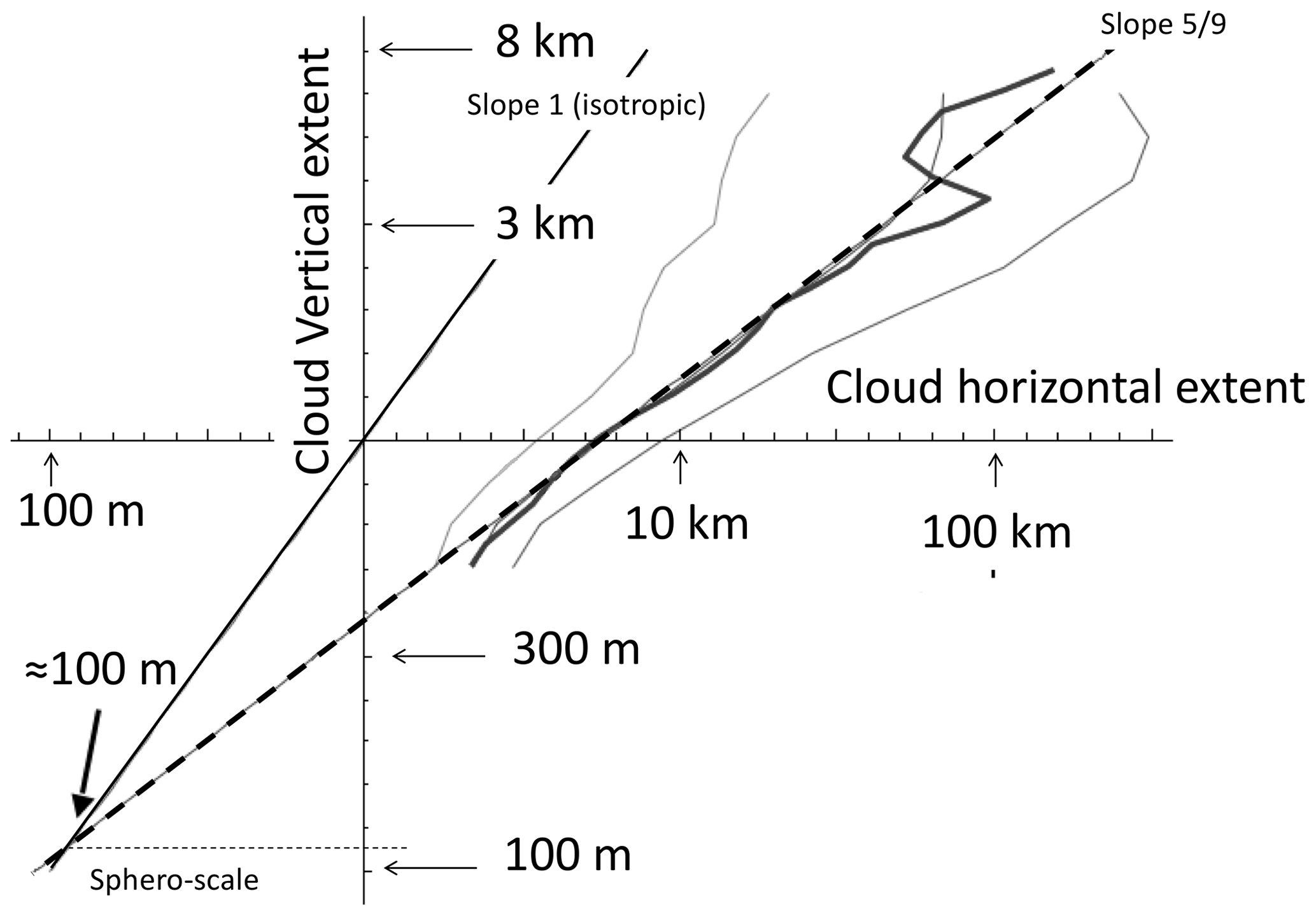
Figure 50A space (horizontal)–space (vertical) diagram estimated from the absolute reflectivity fluctuations (first-order structure functions) from 16 CloudSat orbits. Reproduced from Lovejoy et al. (2009b).
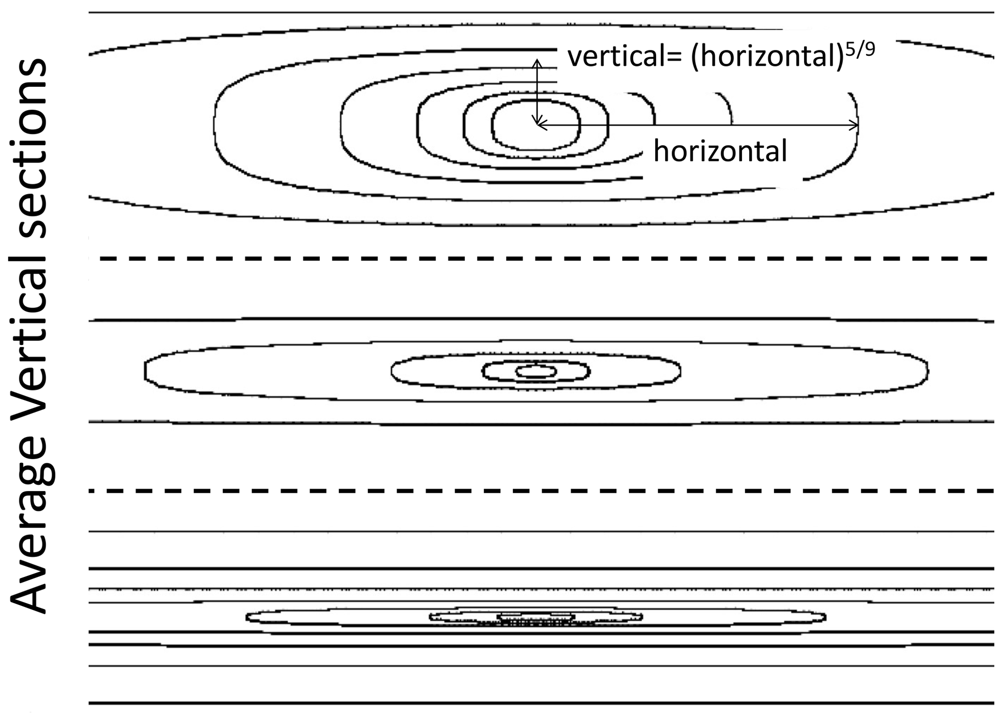
Figure 51The theoretical shapes of average vertical cross sections using the empirical parameters estimated from CloudSat-derived mean parameters: , with spheroscales 1 km (top), 100 m (middle), and 10 m (bottom), roughly corresponding to the geometric mean and 1 standard deviation fluctuations. In each of the three, the distance from left to right horizontally is 100 km, and from top to bottom vertically it is 20 km. It uses the canonical scale function. The top figure in particular shows that structures 100 km wide will be about 10 km thick whenever the spheroscale is somewhat larger than average (Lovejoy et al., 2009c).
Table 3This table uses the estimate of the vertical Hv, the (horizontal) values for Hh for T, logθ, and h (humidity): these are from Lovejoy and Schertzer (2013). For the horizontal velocity v, the aircraft data in Fig. 49 were used. B is the lidar reflectivity (spectral estimate in Fig. 46). For clouds, the far-right column (L) is an estimate using CloudSat cloud length and depth probability data from Guillaume et al. (2018). We find that .

4.2.3 The 23/9D model and numerical weather models
What about numerical weather models? We mentioned that in the horizontal they show excellent scaling (and see Fig. 8 for reanalysis spectra, Fig. 9 for the comparison of Mars and Earth spectra, and Fig. 38 for the cascade structures). According to the 23/9D model, the dynamics are dominated by Kolmogorov scaling in the horizontal () and Bolgiano–Obukhov scaling in the vertical (), so that Assuming that the horizontal directions have the same scaling, typical structures of size L×L in the horizontal have vertical extents of , and hence their volumes are with “elliptical dimension” , the “23/9D model” (Schertzer and Lovejoy, 1985c). Unfortunately, it is nontrivial to test the vertical scaling in models (they are typically based on pressure levels, and their statistics are different than those from true vertical displacements). Nevertheless, an indirect test is to consider the number of vertical levels compared to horizontal levels. In the historical development of NWPs, the number of spatial degrees of freedom – the product of horizontal degrees of freedom multiplied by the vertical number – was limited by computer power. In any given model, the number of vertical levels compared to the number of horizontal pixels is a somewhat ad hoc model choice. However, if we consider (Lovejoy, 2019) the historical development of the models since 1956 (Fig. 52), we see that the number of levels (the vertical range) as a function of the number of zonal degrees of freedom (horizontal range) has indeed followed the power law, so that
Figure 52 shows that the choices of horizontal and vertical scale ranges in the historical development of numerical models are close to the law (and hence to the empirical data), and it contradicts the “standard model” that is based on isotropic symmetries and that attempts to combine a small-scale isotropic 3D regime and a large-scale isotropic (flat) 2D regime in conjunction with a transition supposedly near the atmospheric-scale height of 10 km.
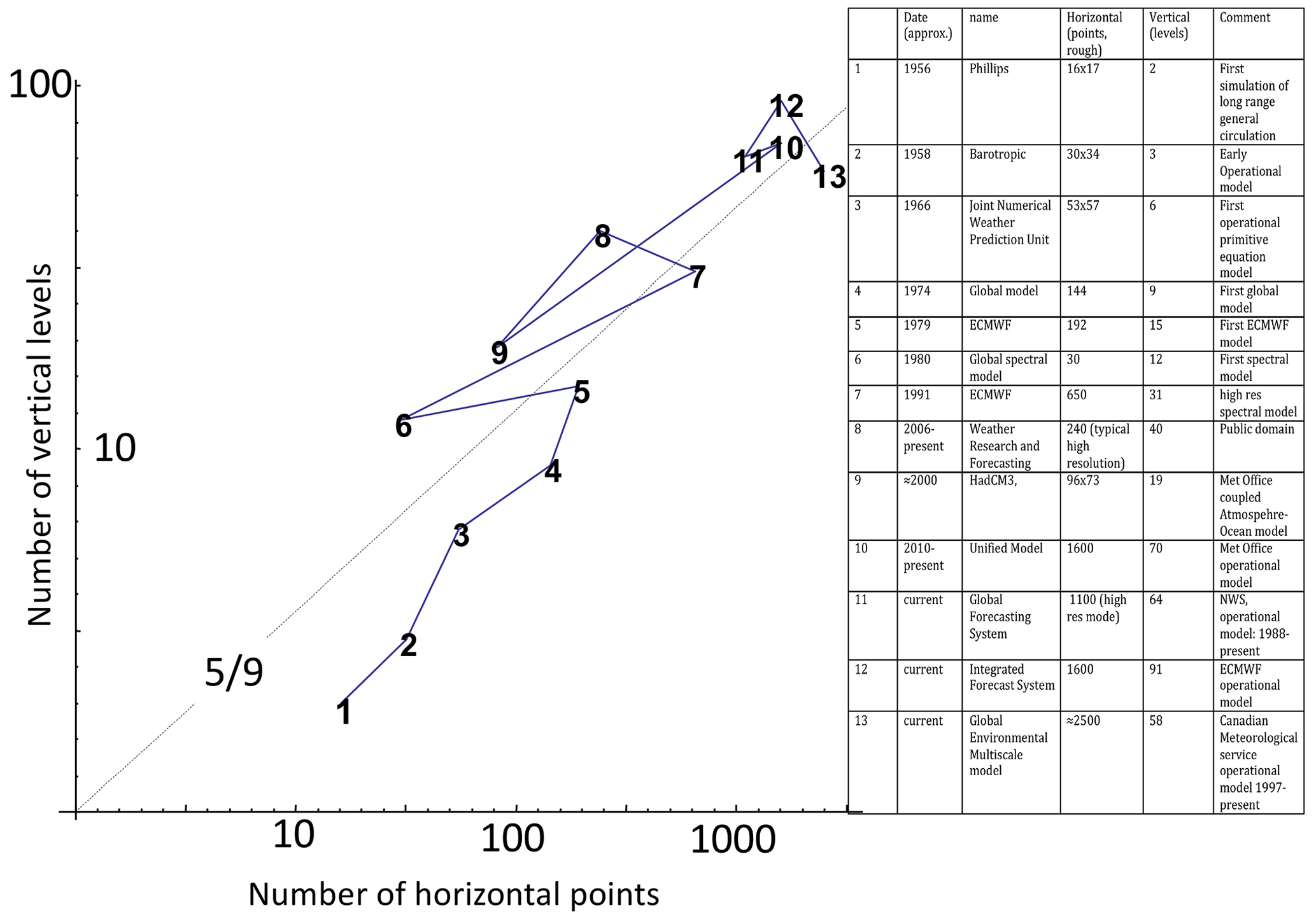
Figure 52The choices of horizontal and vertical numbers of degrees of freedom that were made during the historical development of general circulation models. According to the 23/9D mode I, the dynamics are dominated by Kolmogorov scaling in the horizontal () and Bolgiano–Obukhov scaling in the vertical (), so that Assuming that the horizontal directions have the same scaling, typical structures of size L×L in the horizontal have vertical extents of , and hence their volumes are with “elliptical dimension” , the “23/9D model” (Schertzer and Lovejoy, 1985c). The number of model degrees of freedom thus roughly follows the power of the number of horizontal-resolution (e.g. zonal-resolution) elements. Reproduced from Lovejoy (2019).
4.3 GSI in the horizontal: cloud morphologies, differential rotation, and nonlinear GSI
4.3.1 Differential rotation
Due to the larger north–south temperature gradients, large atmospheric structures 10 000 km in the east–west direction are typically “squashed” to a size about a≈1.6 times smaller in the north–south direction (Sect. 4.1.5). However, there is no systematic change in this aspect ratio as we move to smaller scales, nor is there a plausible theory that might explain one. Although this statement is true of the data, it turns out that one of the limitations of GCMs is that they do have horizontal stratifications that are apparently spurious. If the east–west direction is taken as the reference, GCM structures in the north–south direction follow: (north–south) = (east–west)Hy with Hy=0.80 for this, and for a possible explanation, see Lovejoy and Schertzer (2011).
With this possible exception, we conclude that, unlike the vertical, there is little evidence for any overall stratification in the horizontal analogous to the vertical, but there is still plenty of evidence for the existence of different shapes at different sizes and the fact that shapes commonly rotate by various amounts at different scales. We thus need to go beyond self-affinity and (at least) add some rotation. Mathematically, to add rotation to the blow-up and squashing that we discussed earlier, we only need to add off-diagonal elements to the generator G.
Figures 53–56 show a few examples of contours at different scales, each representing the shapes of the balls at systematically varying scales. We can see that we have the freedom to vary the unit balls (here circles and rounded triangles) and the amounts of squashing and rotation. In Fig. 53, with unit balls taken to be circles, we show the self-similar case in the upper left, a stratified case in the upper right, a stratified case with a small amount of rotation (lower left), and another case with lots of rotation (lower right). Figure 56 shows the same but with unit balls as rounded triangles, Fig. 55 takes the lower-right example and displays the balls over a factor of 1 billion in scale, and in Fig. 56 we show an example with only a little rotation but over the same factor of 1 billion in scale. We can see that, if these represent average morphologies of clouds at different scales, even though there is a single unique rule or mechanism to go from one scale to another, the average shapes change quite a bit with scale.
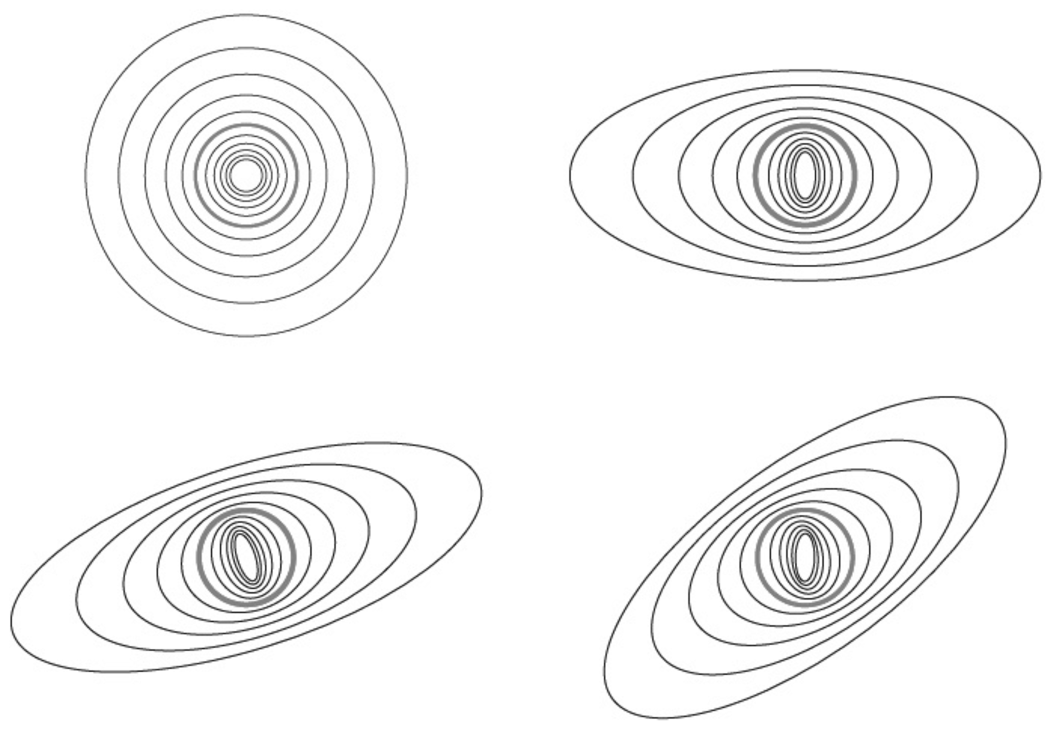
Figure 53Blow-ups and reductions by factors of 1.26 starting at circles (red). The upper left shows the isotropic case, the upper right shows the self-affinity (pure stratification case), the lower-left example is stratified but along oblique directions, and the lower-right example has structures that rotate continuously with scale while becoming increasingly stratified. The matrices used are , , , and (upper left to lower right). Reproduced from Lovejoy (2019).
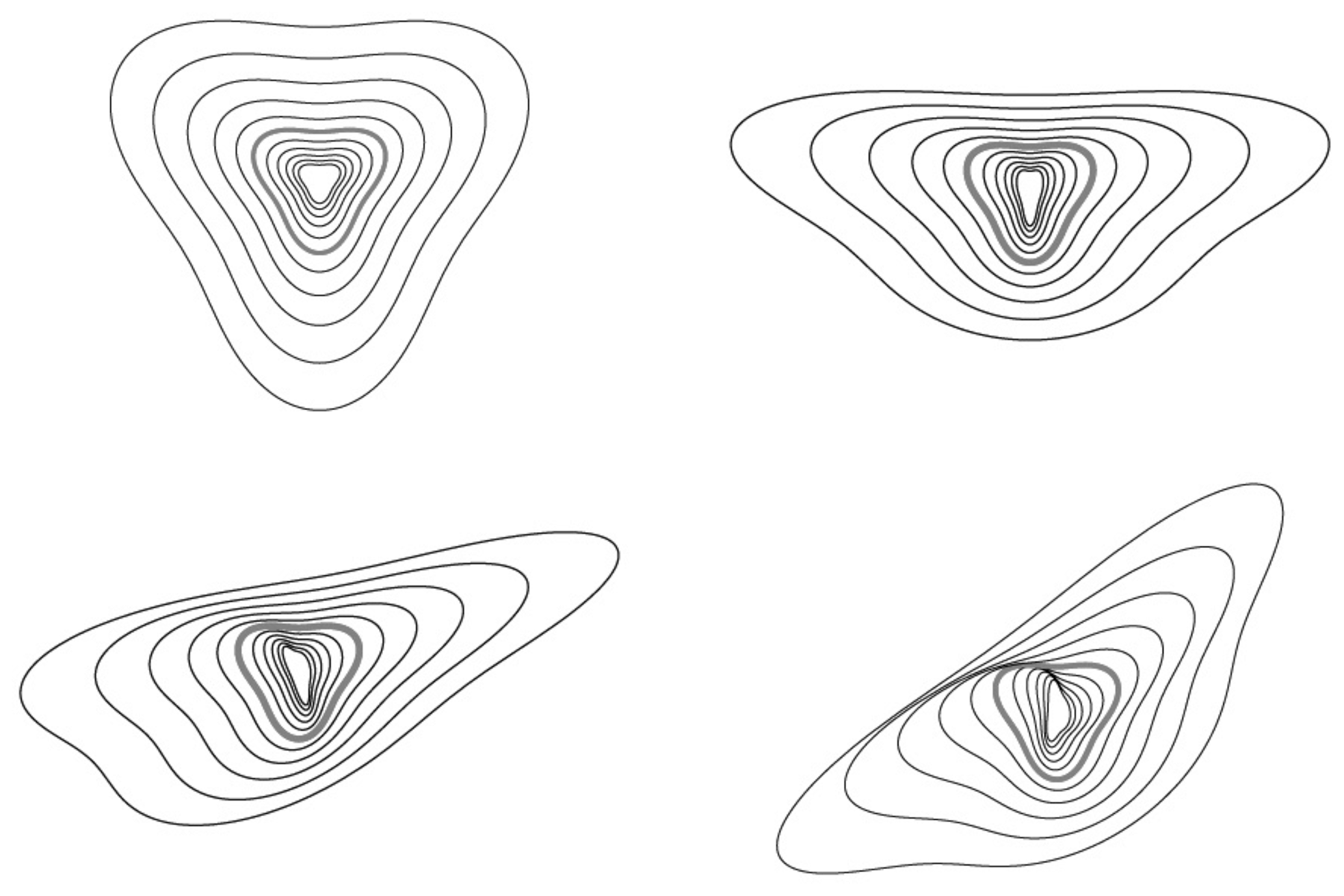
Figure 54The same as above except that now the unit ball is the rounded triangle. Reproduced from Lovejoy (2019).
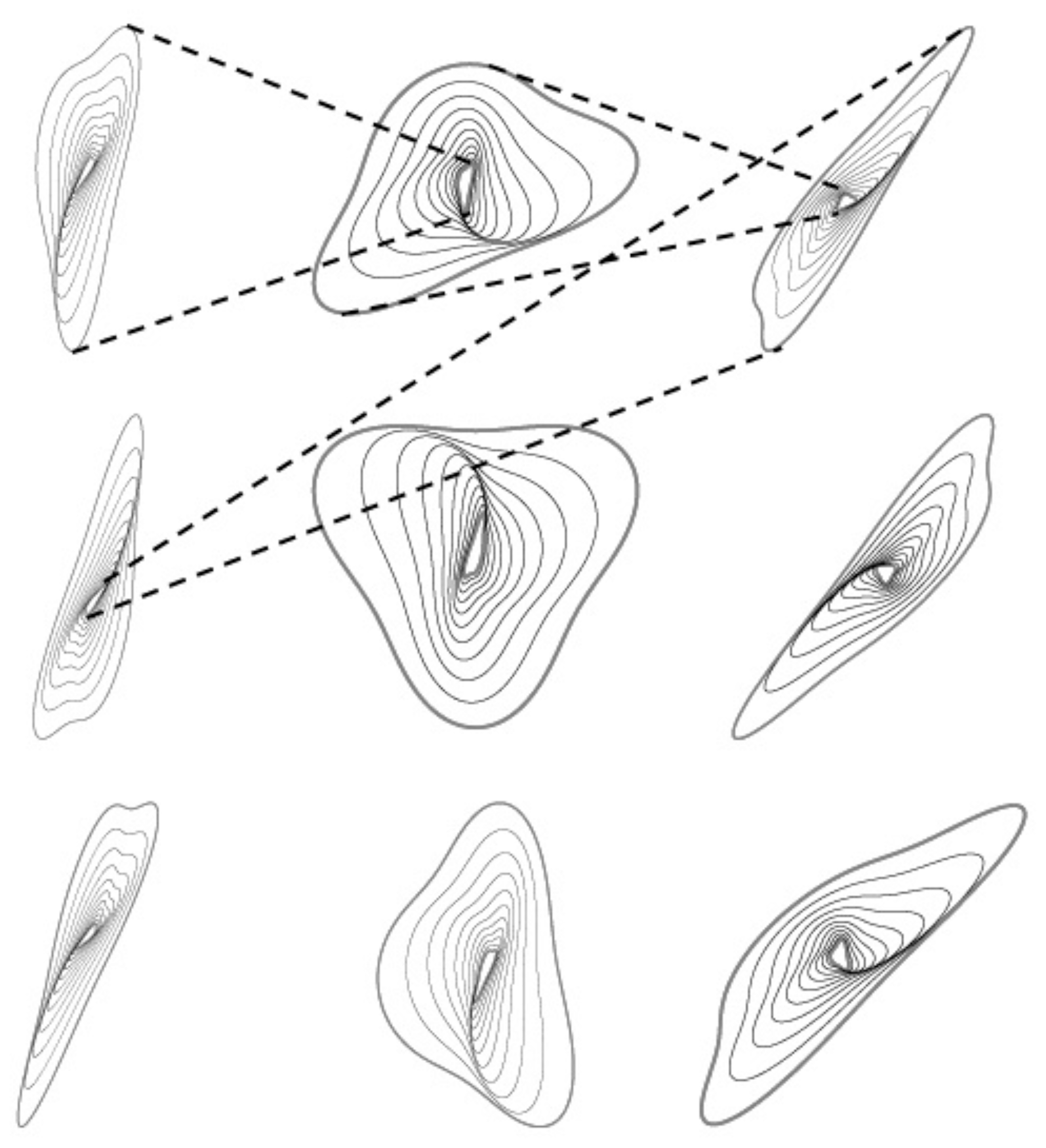
Figure 55The same blow-up rule as in the lower right of Fig. 53 but showing an overall blow-up by a factor of 1 billion. Starting with the inner thick grey ball in the upper-left corner, we see a series of 10 blow-ups, each by a factor of 1.26 spanning a total of a factor of 10 (the outer thick, grey ball). Then, that ball is shrunk (as indicated by the dashed lines) so as to conveniently show the next factor of 10 blow-up (top middle). The overall range of scales in the sequence is thus 109= 1 billion. The scale-changing rule (matrix) used here is the same as the lower right in Figs. 53 and 54: . Reproduced from Lovejoy (2019).
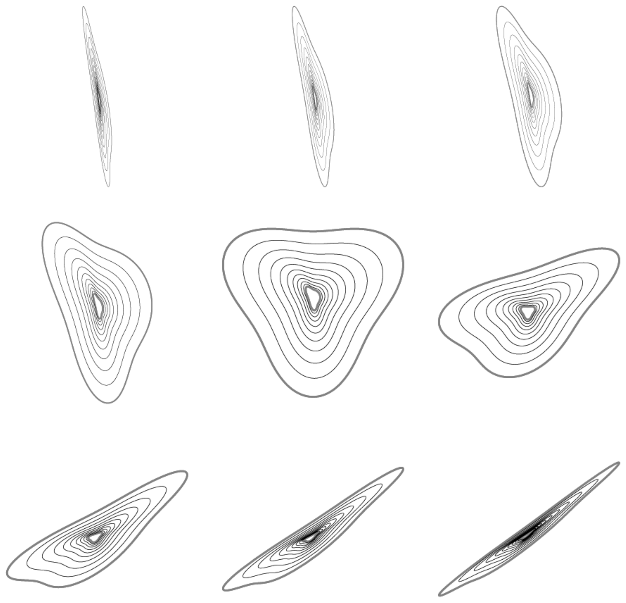
Figure 56A different example of balls with squashing but with only a little rotation: the maximum rotation of structures in this example from very small to very large scales is 55∘. The matrix used here was . Reproduced from Lovejoy (2019).
4.3.2 Anisotropic multifractal clouds
We have explored ways in which quite disparate shapes can be generated using blow-ups, squashings, and rotations. With the help of a unit ball, we generated families of balls, any member of which would have been an equally good starting point. The unit ball has no particular importance, and it does not have any special physical role to play. If we have a scaling model based on isotropic balls, then replacing them with these anisotropic balls will also be scaling when we use the anisotropic rule to change scales: any morphologies made using such a system of balls will be scale-invariant. Mathematically anisotropic space–time models (see Schertzer and Lovejoy, 1987; Wilson et al., 1991; Lovejoy and Schertzer, 2010b, a) are produced in the same way as isotropic ones, except that the usual vector norm is replaced by a spacescale and timescale function and the usual dimension of space–time D (4) is replaced by Del:
where .
We already showed a self-similar and stratified example where the balls were used to make a multifractal cloud simulation of a vertical section (Fig. 5). Let us now take a quick look at a few examples of horizontal and 3D multifractal cloud simulations.
The simulation of a cross section of a stratified multifractal cloud in Fig. 5 already shows that the effect of changing the balls can be quite subtle. Let us take a look at this by making multifractal cloud simulations with realistic (observed) multifractal parameters (these determine the fluctuation statistics, not the anisotropy) and systematically varying the families of balls (Fig. 57). In the figure, all the simulations have the same random “seed”, so that the only differences are due to the changing definition of scale. First we can explore the effects of different degrees of stratification combined with different degrees of rotation. We consider two cases: in the first (Fig. 57), there is roughly a circular unit ball within the simulated range, and in the second (Fig. 58), all the balls are highly anisotropic. Each figure shows a pair: the cloud simulation (left) and the family of balls that were used to produce it on the right.
From the third column in Fig. 57 with no stratification, we can note that changing the amount of rotation (moving up and down the column) changes nothing; this is simply because the circles are rotated to circles: rotation is only interesting when combined with stratification. The simulations in Fig. 58 might mimic small clouds (for example 1 km across) produced by complex cascade-type dynamics that started rotating and stratifying at scales perhaps 10 000 times larger. In both sets of simulations, the effect of stratification becomes more important up and down away from the centre line, and the effects of rotation vary from the left to the right, becoming more important as we move away from the third column.
Figure 59 shows examples where rotation is strong and the scale-changing rule is the same everywhere; only the unit ball is changed. By making the latter have some long narrow parts, we can obtain quite “wispy”-looking clouds.
Figure 60 shows another aspect of multifractal clouds. In Sect. 3.5.5 we discussed the fact that, in general, the cascades occasionally produce extreme events. If we make a sufficiently large number of realizations of the process, from time to time we will generate rare cloud structures that are almost surely absent on typical realizations. For example, a typical satellite picture of the tropical Atlantic Ocean would not have a hurricane, but from time to time hurricanes do appear there. The multifractality implies that this could happen quite naturally, without the need to invoke any special scalebound “hurricane process”. In the examples in Fig. 60, we use a rotating set of balls (Fig. 61). However, in order to simulate occasional, rare realizations, we have “helped” the process by artificially boosting the values in the vicinity of the central pixel. The two different rows are identical except for the sequence of random numbers used in their generation. For each row, moving from left to right, we boosted only the central region to simulate stronger and stronger vortices that are more and more improbable. As we do this, we see that the shapes of the basic set of balls begin to appear out of the chaos.
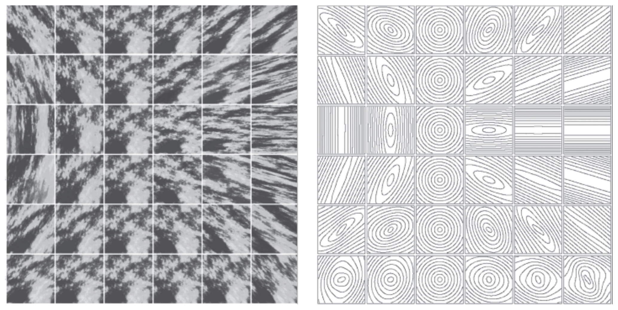
Figure 57Left: multifractal simulations with nearly isotropic unit scales with stratification becoming more important up and down away from the centre line and the rotation parameter (left to right) becoming more important as we move away from the third column. Right: the balls used in the simulations to the left. This is an extract from the multifractal explorer website: http://www.physics.mcgill.ca/~gang/multifrac/index.htm (last access: 3 July 2023). Reproduced from Lovejoy and Schertzer (2007b).
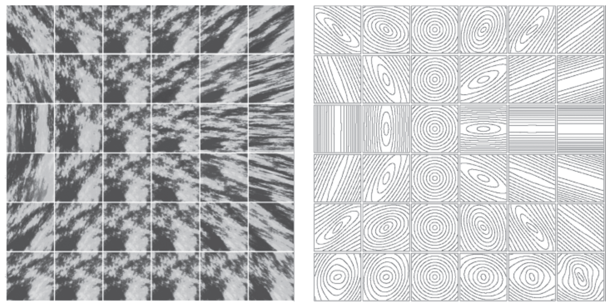
Figure 58The same as above except that the initial ball is highly anisotropic in an attempt to simulate the effect of stretching due to a wide range of larger scales. Reproduced from Lovejoy and Schertzer (2007b).
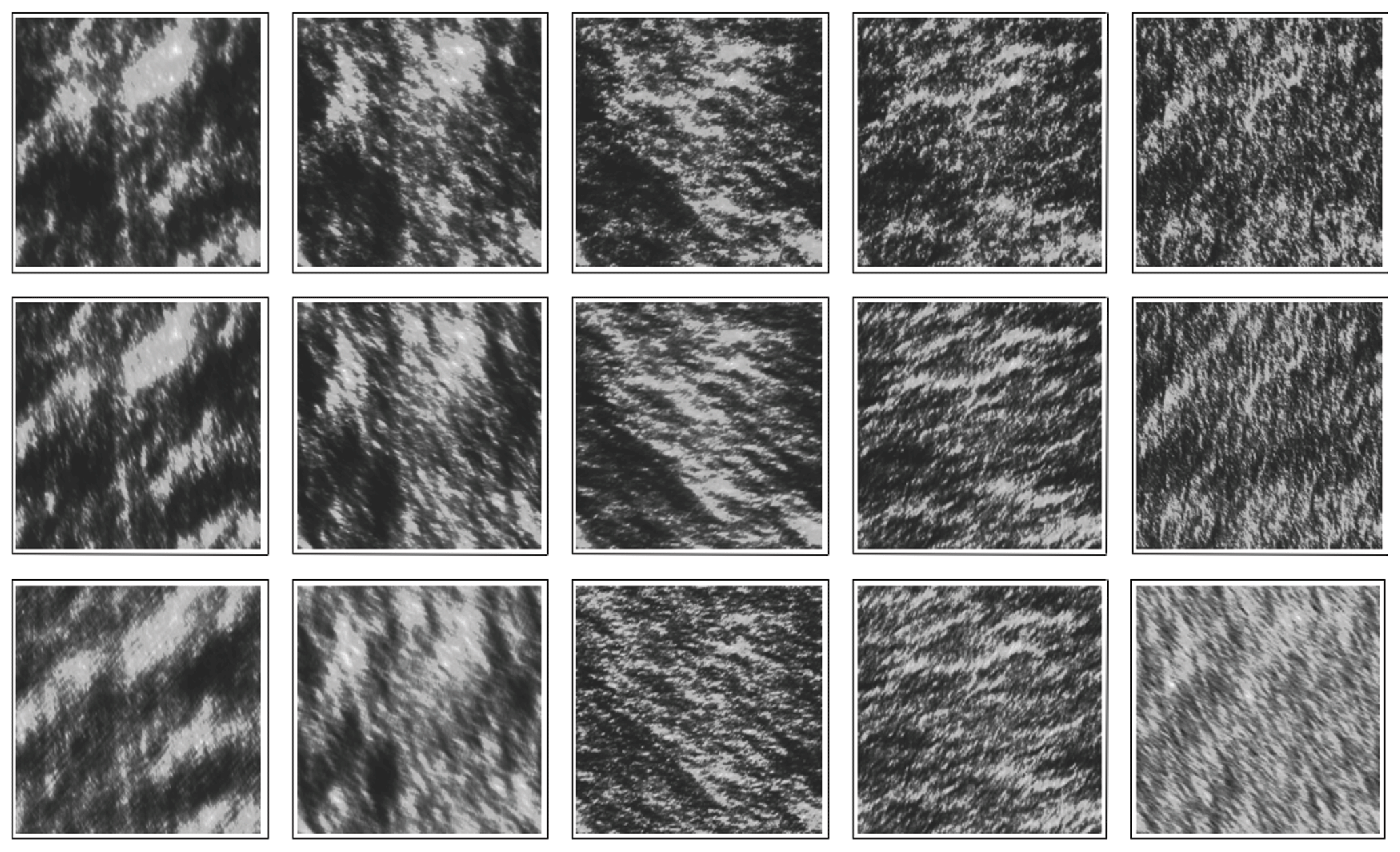
Figure 59Simulations of cloud liquid water density with the scale-changing rule the same throughout: only the unit balls are systematically modified so as to yield more and more “wispy” clouds. Reproduced from Lovejoy et al. (2009).
4.3.3 Radiative transfer in multifractal clouds
The cloud simulations above are for the density of cloud liquid water; they used false colours to display the more and less dense cloud regions. Real clouds are of course in 3D space, and the eye sees the light that has been scattered by the drops. Therefore, if we make 3D cloud simulations, instead of simply using false colours, we can obtain more realistic renditions by simulating the way light interacts with the clouds (see Figs. 8, 25, and 26 for various scaling analyses of cloud radiances at various wavelengths). The study of radiative transfer in multifractal clouds is in its infancy; see however Naud et al. (1997), Schertzer et al. (1997b), Lovejoy et al. (2009d), and Watson et al. (2009).
Figures 61 and 62 show the top and side views of a multifractal cloud with the usual false colours; Figs. 64 and 65 show the same cloud rendered by simulating light travelling through the cloud with both top (Fig. 64) and bottom (Fig. 65) views. Finally, in Fig. 66, we show a simulation of thermal infrared radiation emitted by the cloud, similar to what can observed from infrared weather satellites. We see that quite realistic morphologies are possible.
Up until now, we have only discussed space, but of course clouds and other atmospheric structures evolve in time. Since we have argued that the wind field is scaling and the wind moves clouds around, it effectively couples space and time. We therefore have to consider scaling in space and in time: in space–time. The time domain opens up a whole new realm of possibilities for simulations and morphologies. While the balls in space must be localized – since they represent typical spatial structures, “eddies” – in space–time they can be delocalized and form waves. In this case it turns out that it is easier to describe the system using the Fourier methods. Figure 67 shows examples of what can be achieved with various parameters.
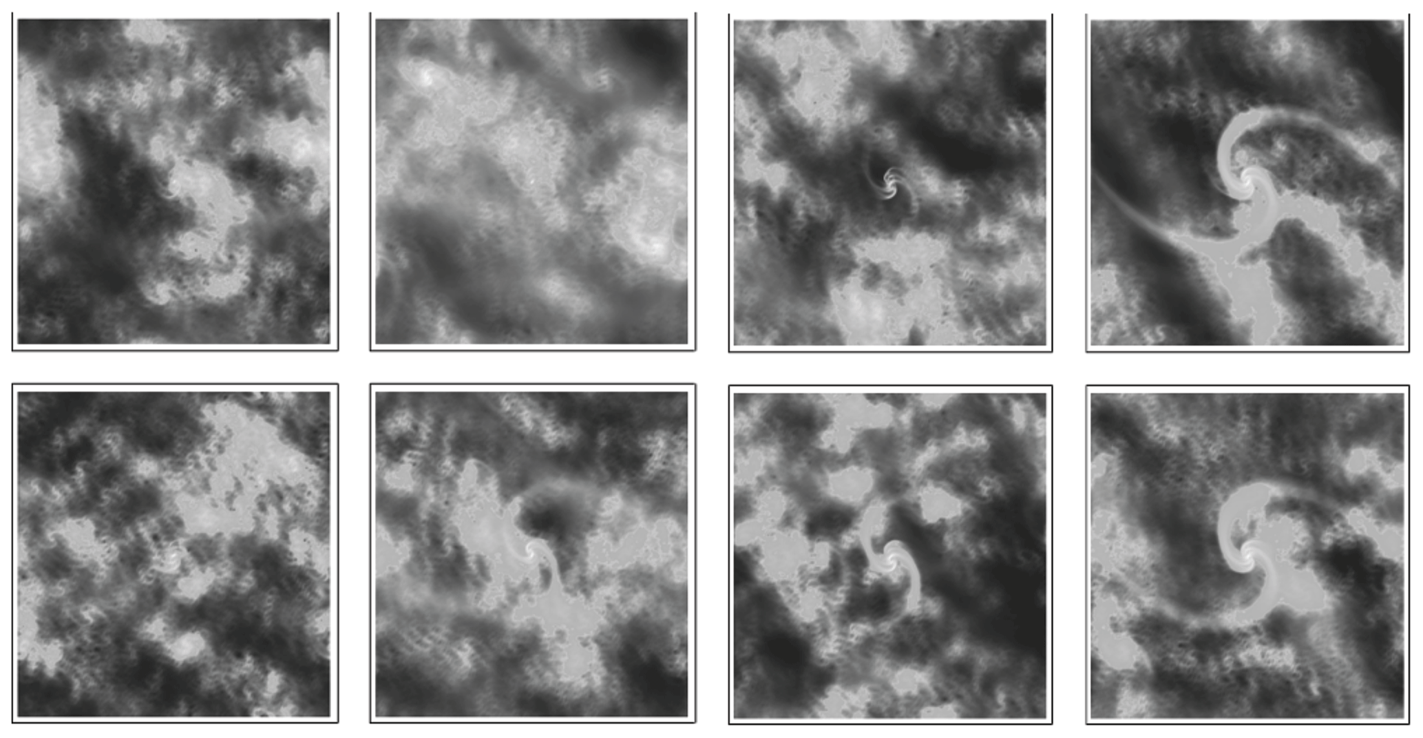
Figure 60Each row has a different random seed but is otherwise identical. Moving from left to right shows a different realization of a random multifractal process, with the central part boosted by factors increasing from left to right in order to simulate very rare events. The balls are shown in Fig. 61. Reproduced from Lovejoy and Schertzer (2013).
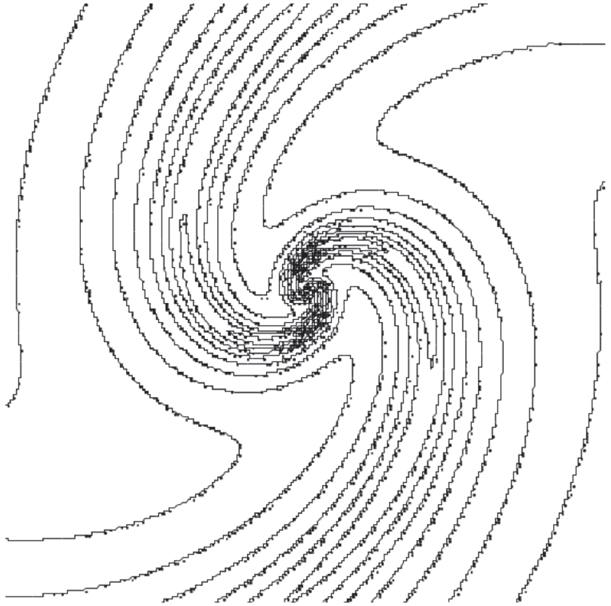
Figure 61The balls used in the simulations above. Contours of the (rotation-dominant) scale function used in the simulations in Fig. 60. Reproduced from Lovejoy and Schertzer (2013).
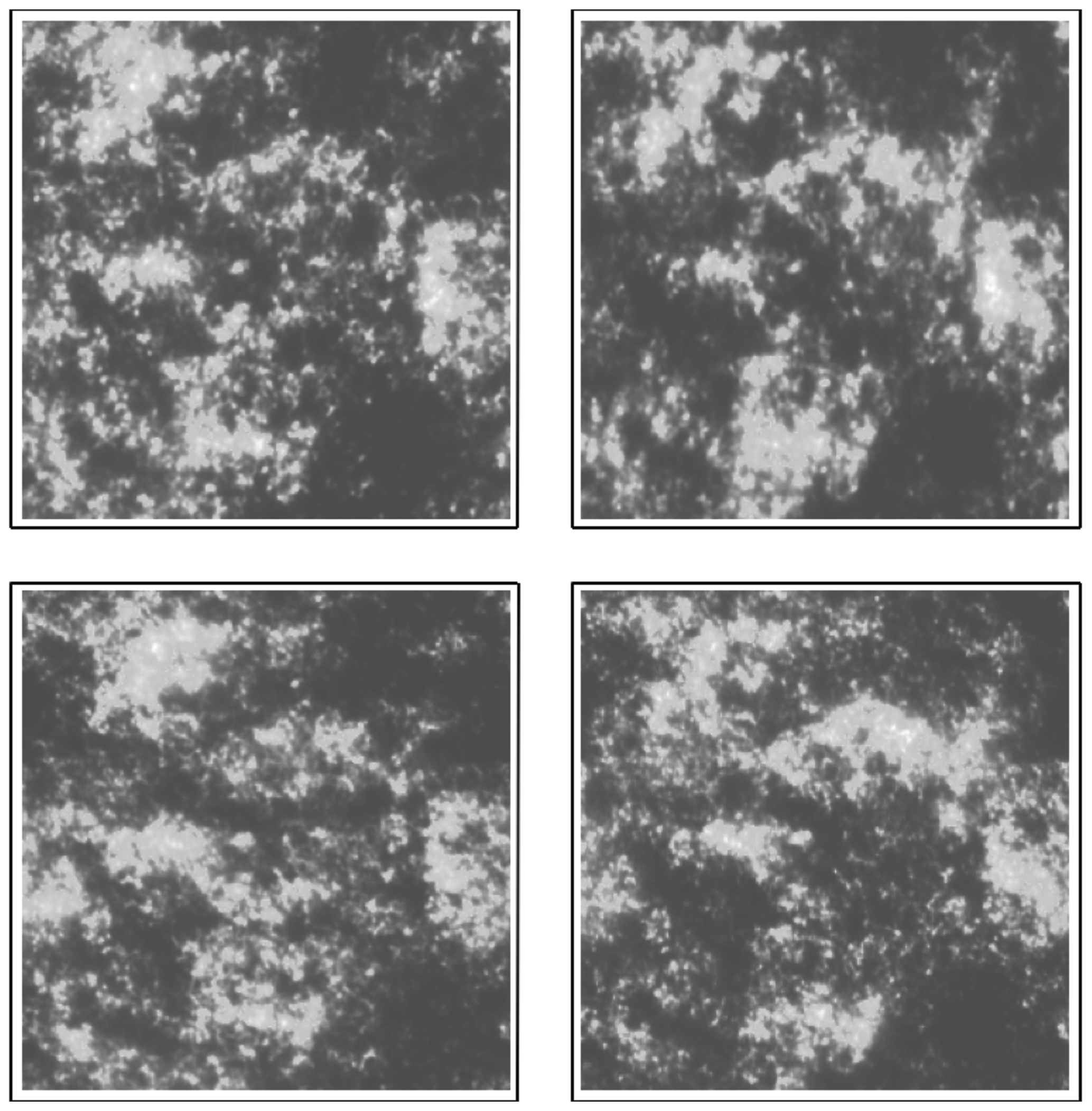
Figure 62The top layer of cloud liquid water using a grey-shaded rendition. Reproduced from Lovejoy and Schertzer (2013).
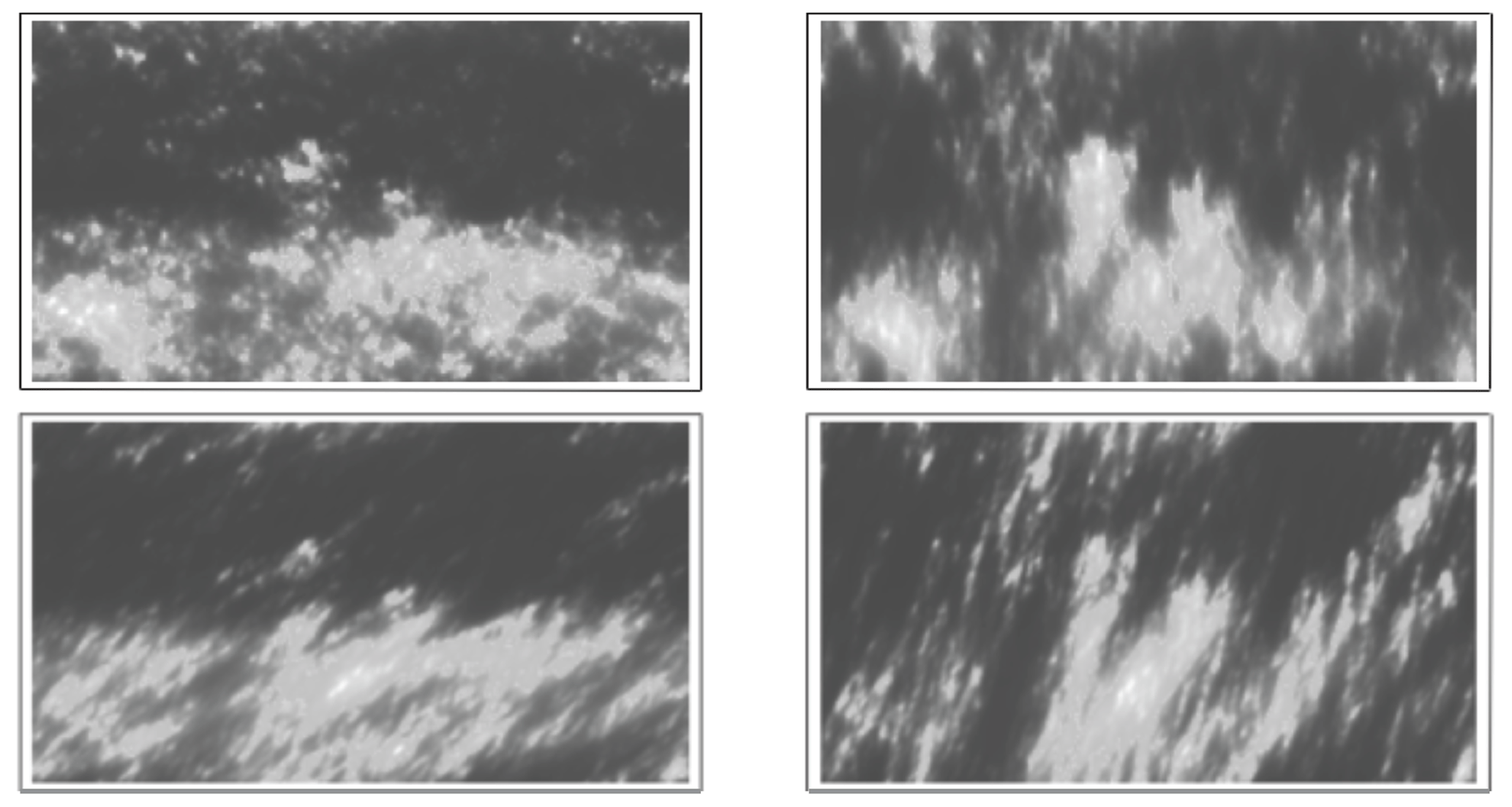
Figure 63A side view of the previous one. Reproduced from Lovejoy and Schertzer (2013).
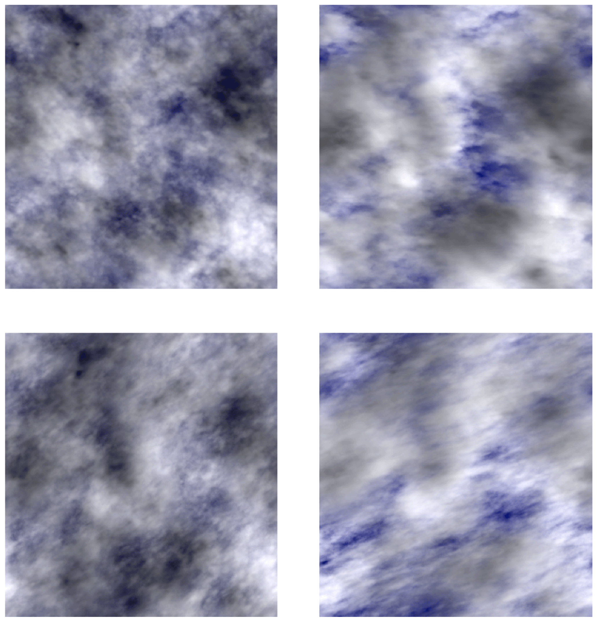
Figure 64The top view with light scattering for the Sun (incident at 45∘ to the right). Reproduced from Lovejoy and Schertzer (2013).
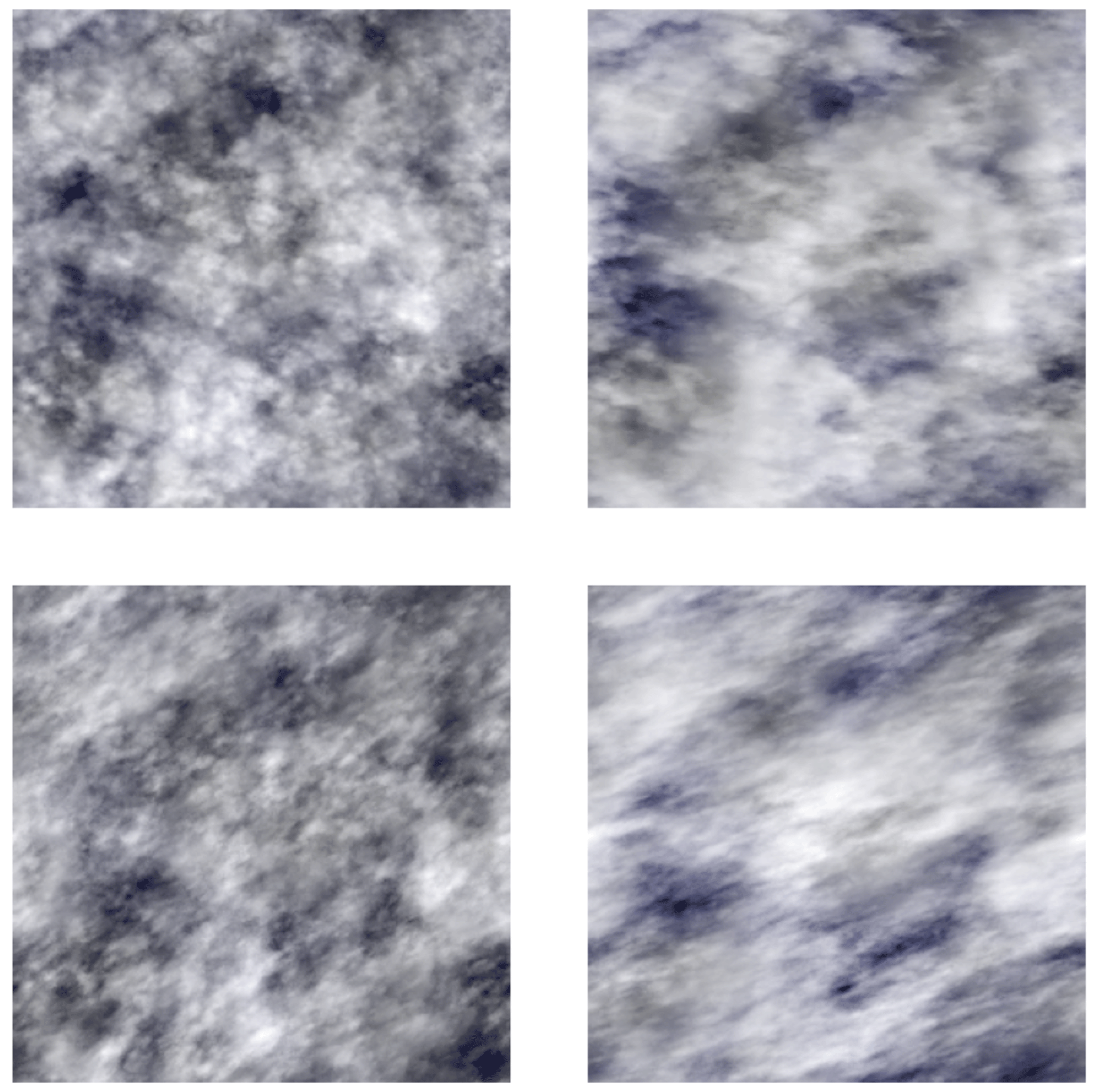
Figure 65The same as Fig. 64 except viewed from the bottom. Reproduced from Lovejoy and Schertzer (2013).
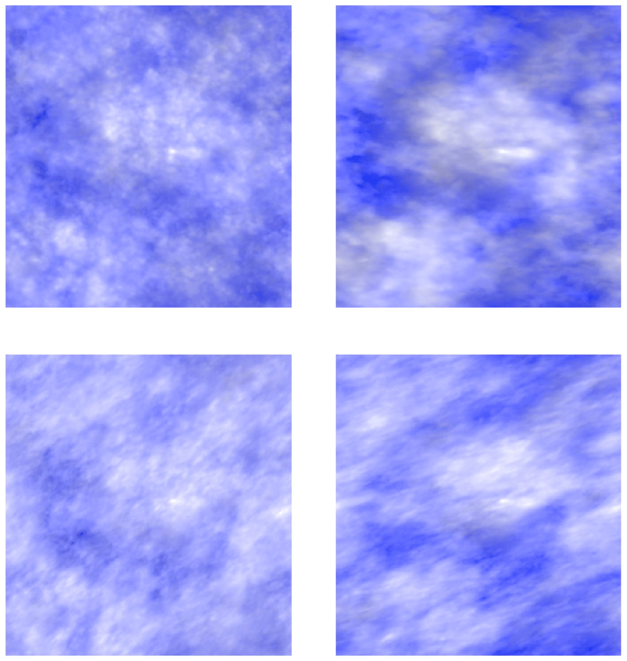
Figure 66The same as Fig. 64 except for a grey-shaded rendition of a thermal infrared field as might be viewed by an infrared satellite. Reproduced from Lovejoy and Schertzer (2013).
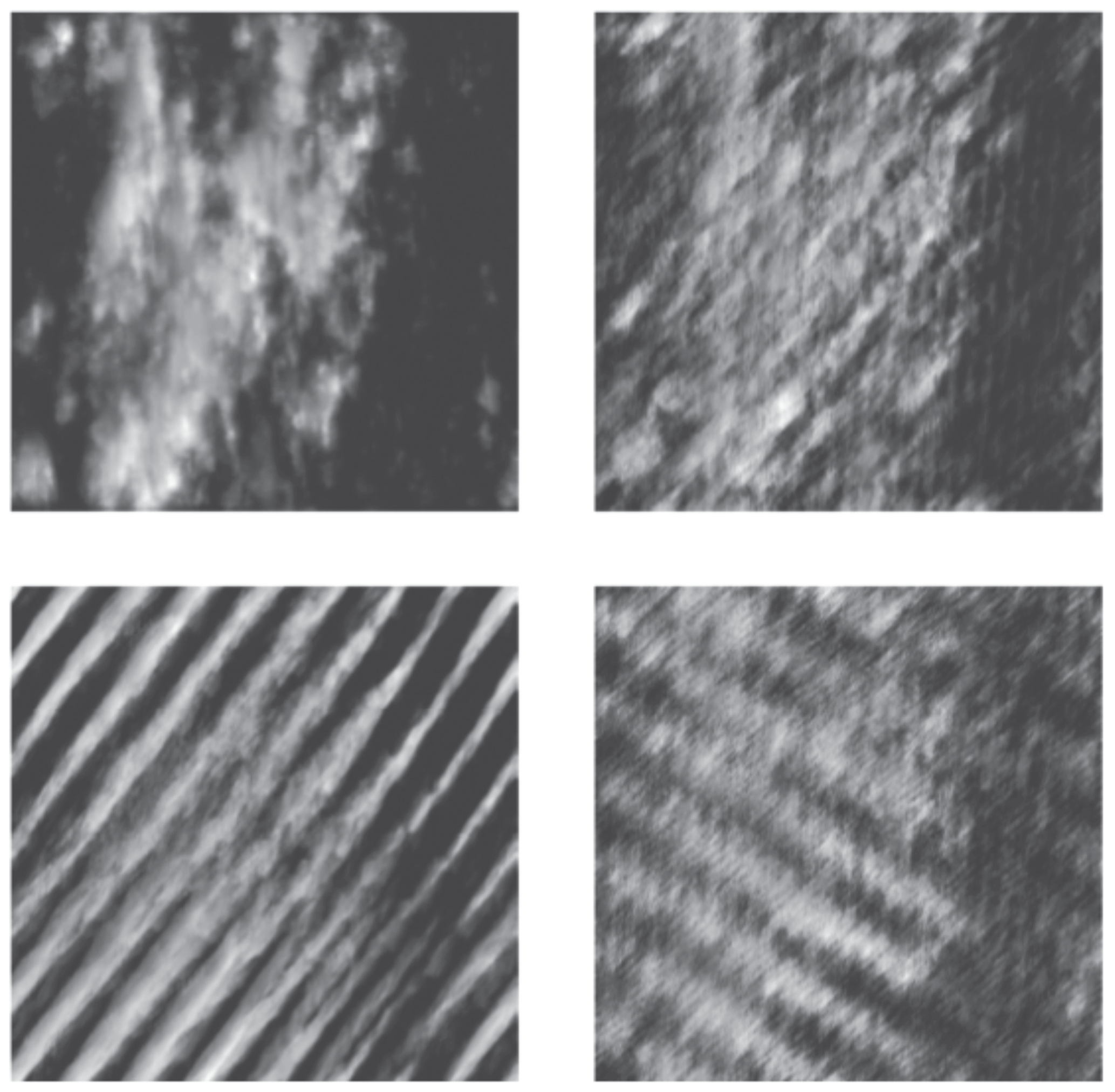
Figure 67Examples of simulations in space–time showing wavelike morphologies. The same basic shapes are shown but with the wavelike character increasing clockwise from the upper left. Reproduced from the reference Lovejoy et al. (2008b).
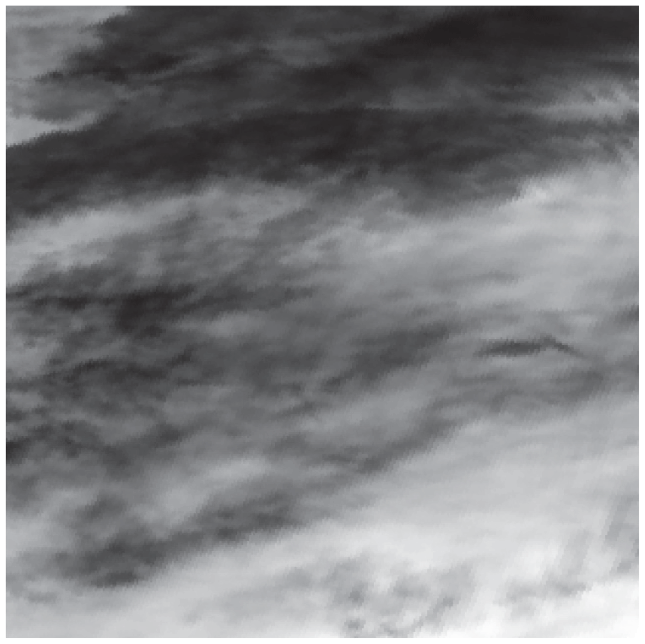
Figure 68An infrared satellite image from a satellite at 1.1 km resolution, 512×512 pixels. Reproduced from Lovejoy and Schertzer (2013).
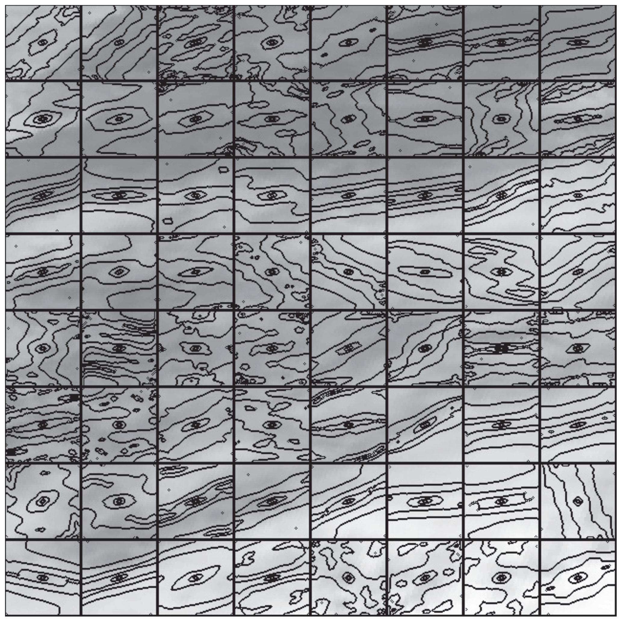
Figure 69Estimates of the shapes of the balls in each 64×64-pixel box from the image in Fig. 68. Reproduced from Lovejoy and Schertzer (2013).
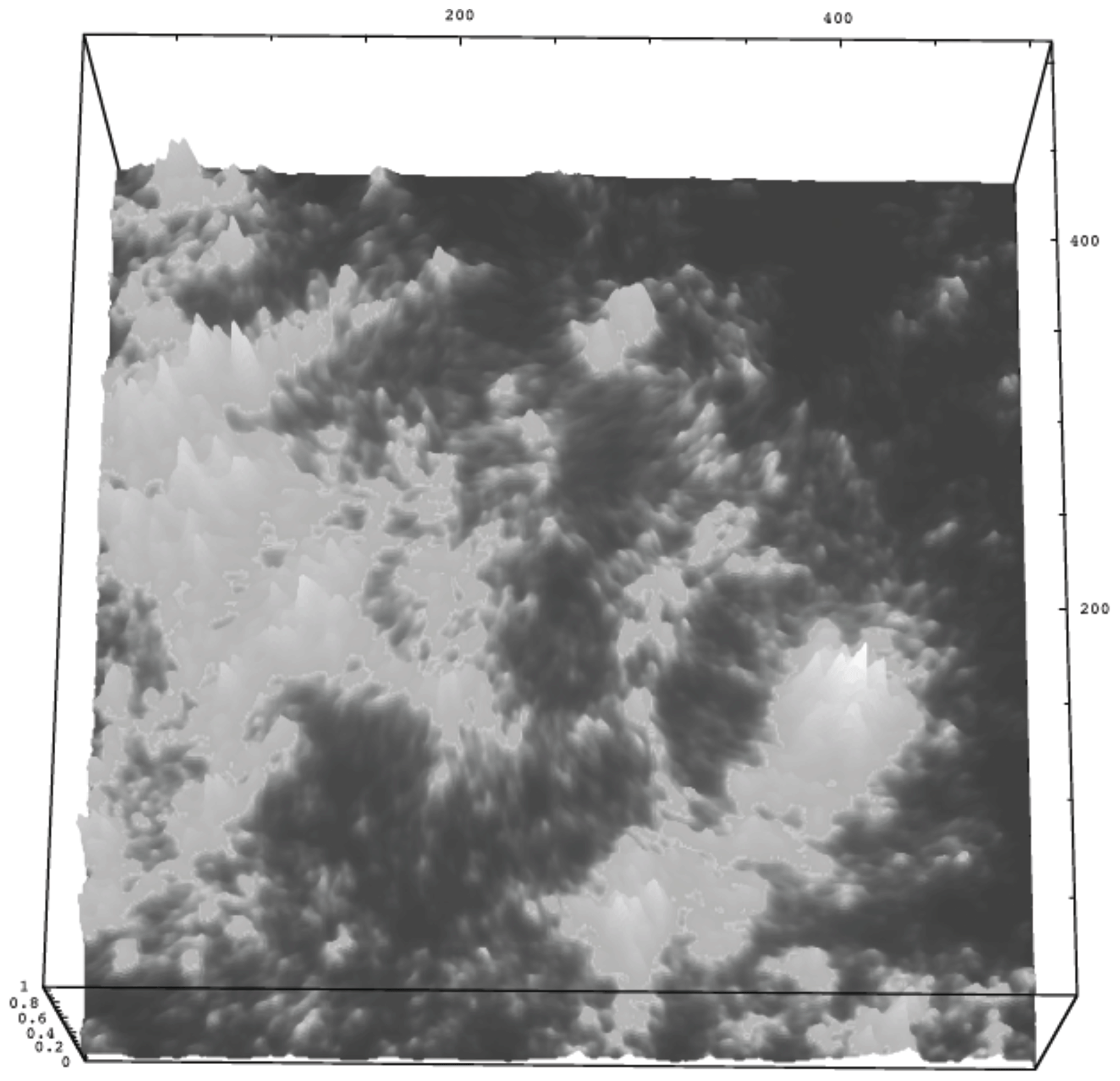
Figure 70A multifractal simulation of a cloud with texture and morphology varying in both location and scale, simulated using nonlinear GSI; the anisotropy depends on both scale and position according to the balls shown in Fig. 71. Reproduced from Lovejoy and Schertzer (2013).
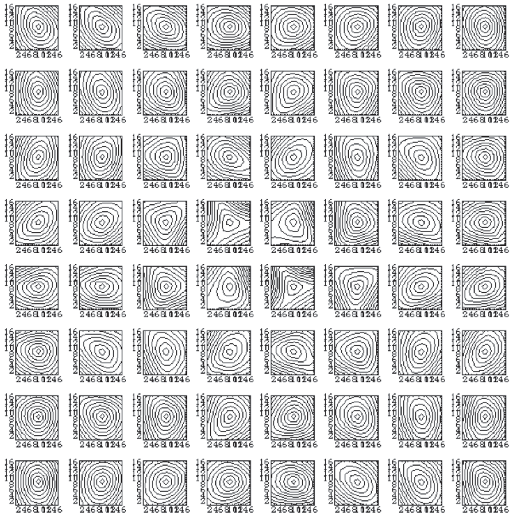
Figure 71The set of balls displayed according to their relative positions used in the simulation shown in Fig. 70. Reproduced from Lovejoy and Schertzer (2013).
4.3.4 Nonlinear GSI: anisotropy that changes from place to place and from scale to scale
Generalized scale invariance is necessary since zooming into clouds displays systematic changes in morphology with the magnification, so that in order to be realistic, we needed to generalize the idea of self-similar scaling. The first step was to account for the stratification. When the direction of the stratification is fixed (pure stratification), there is no rotation with scale. We saw that, to model the horizontal plane, we needed to add rotation and, to a first approximation, we could think of the different cloud morphologies as corresponding to different cloud types – cumulus, stratus, cirrus, etc.
However, there is still a problem. Up until now, we have discussed linear GSI where the generator is a matrix, so that the scale-changing operator λ−G is also a linear transformation. Now we need to generalize this to account for the fact that because cloud types and morphologies not only change with scale, they also change with spatial location (and in time). Figure 66 shows the problem with a real satellite infrared cloud picture: it seems clear that the textures and morphologies vary from one part of the image to another. Using a type of 2D fluctuation analysis, we can try to estimate the corresponding “balls”. When the image is broken up into an 8×8 array of sub-images (Fig. 69, with a fair bit of statistical scatter), we can confirm that the balls are quite different from one place to another.
In the more general nonlinear GSI, the notion of scale depends not only on the scale, but also on the location. In nonlinear GSI we introduce the generator of the infinitesimal scale change (consider just space and use the notation , x2, x3)). Using , we can obtain the following equation for the scale function:
(summation over repeated indices).
Locally (in a small enough neighbourhood of a point), linear GSI is defined by the tangent space; i.e. the elements of the linear generator are
In the special case of linear GSI, this yields
Full details and more examples are given in Chap. 7 of Lovejoy and Schertzer (2013).
Figures 70 and 71 show an example. The physics behind this are analogous to those in Einstein's theory of general relativity. In the latter, it is the distribution of mass and energy in the universe that determines the appropriate notion of distance, i.e. the metric. With GSI, it is the nonlinear turbulent dynamics that determine the appropriate notions of scale and size. Note however an important difference: the GSI notion of scale is generally not a metric; it is not a distance in the mathematical sense.
With nonlinear GSI a bewildering variety of phenomena can be described in a scaling framework. The framework turns out to be so general that it is hard to make further progress. It is like saying “the energy of the atmosphere is conserved”. While this is undoubtedly true – and this enables us to reject models that fail to conserve it – this single energy symmetry is hardly adequate for modelling and forecasting the weather. One can imagine that, if one must specify the anisotropy both as a function of scale and as a function of location, many parameters are required. At a purely empirical level, these are difficult to estimate since the process has such strong variability and intermittency. In order to progress much further, we will undoubtedly need new ideas. However, the generality of GSI does make the introduction of scalebound mechanisms unnecessary.
4.3.5 The scalebound approach and the phenomenological fallacy
We have given the reader a taste of the enormous diversity of cloud morphologies that are possible within the scaling framework. We discussed morphologies that were increasingly stratified at larger scales, that rotated with scale but only a bit, or that rotated many times. There were filamentary structures, there were structures with waves, and there were structures whose character changed with position. Although all of these morphologies changed with scale, they were all consequences of dynamical mechanisms that were scale-invariant. The scalebound approach is therefore logically wrong and scientifically unjustified. When scalebound mechanisms and models based solely on phenomenological appearances are invoked, they commit a corollary of the scalebound approach: the “phenomenological fallacy” (Lovejoy and Schertzer, 2007c). More concisely, the phenomenological fallacy is the inference of mechanisms from phenomenology (appearances).
Starting in the 1970s, deterministic chaos, scaling, and fractals have transformed our understanding of many nonlinear dynamical systems including the atmosphere: they were the main components of the “nonlinear revolution”. While deterministic chaos is largely a deterministic paradigm with a small number of degrees of freedom, the scaling, fractal, and later multifractal paradigm is a stochastic framework with a large number of degrees of freedom that is particularly appropriate to the atmosphere. Ever since Richardson proposed his law of turbulent diffusion in the 1920s, scaling has been explicit and central in turbulence theories. Scaling and multifractals therefore embody the modern turbulent strand of atmospheric science. Over the last century, deterministic and stochastic strands of atmospheric science have developed largely in parallel. The first, “dynamical meteorology”, is an essentially mechanistic, phenomenologically based approach: it is largely scalebound because the relevant processes were believed to occur over narrow ranges of scales. Since atmospheric variability occurs over a wide range of scales, a large number of such processes are required. The second, a statistical turbulence approach, is by contrast based on the scaling idea that there exists a simple statistical relation between structures and processes at potentially widely different scales – unique dynamical regimes spanning wide ranges of scale. However, the classical turbulence notion of scaling is highly restrictive. For one, it assumes that processes are not far from Gaussian, whereas real-world turbulence is by contrast highly intermittent. For another, it reduces scaling to its isotropic special case “self-similarity” – effectively confounding the quite different scale and direction symmetries.
Without further developments, neither classical approach is a satisfactory theoretical framework for atmospheric science. Fortunately, by the turn of the millennium, numerical models – based on the scaling governing equations – had matured to the point that they were increasingly – and today, often exclusively – being used to answer atmospheric questions. As a consequence, the deficiencies of the classical approaches are thus increasingly irrelevant for applied atmospheric science. However, there are consequences: elsewhere (Lovejoy, 2022a), I have argued that the primary casualty of the disconnect between high-level atmospheric theory and empirical science is that it blinds us to potentially promising new approaches. If only to reduce the current large (and increasing) uncertainties in projection projections, new approaches are indeed urgently needed.
This review therefore focuses on the new developments in scaling that overcame these restrictions: multifractals to deal with scaling intermittency (Sect. 3) and generalized scale invariance (Sect. 4) to deal with scaling stratification and more generally scaling anisotropy. GSI clarifies the significance of scaling in geoscience since it shows that scaling is a rather general symmetry principle: it is thus the simplest relation between scales. Just as the classical symmetries (temporal, spatial invariance, directional invariance) are equivalent (Noether's theorem) to conservation laws (energy, momentum, angular momentum), the (nonclassical) scaling symmetry conserves the scaling exponents G,K, and c. Symmetries are fundamental since they embody the simplest possible assumption or model: under a change in the system, there is an invariant. In physics, initial assumptions about a system are that it respects symmetries. Symmetry breaking is only introduced on the basis of strong evidence or theoretical justification: in the case of scale symmetries, one only introduces characteristic space scales or timescales when this is absolutely required.
There are now massive data analyses of all kinds – including ones based on new techniques, notably trace moments and Haar fluctuations – that confirm and quantify atmospheric scaling over wide ranges in the horizontal and vertical. Since this includes the wind field, this implies that the dynamics (i.e. in time) are also scaling. Sections 1 and 2 discuss how, over the range of milliseconds to at least hundreds of millions of years, temporal scaling objectively defines five dynamical ranges: weather, macroweather, climate, macroclimate, and megaclimate. The evolution of the scalebound framework from the 1970s (Mitchell) to the 2020s (Von der Leyden et al.) shows that it is further and further divorced from empirical science. This is also true of the usual interpretation of space–time (Stommel) diagrams that are re-interpreted in a scaling framework (Sect. 2.6). These scalebound frameworks have survived because practising atmospheric scientists increasingly rely instead on general circulation models that are based on the primitive dynamical equations. Fortunately, the outputs of these models inherit the scaling of the underlying equations and are hence themselves scaling: they can therefore be quite realistic. For decades, this has allowed the contradiction between the scaling reality and the dominant “mental model” to persist.
Similar comments apply to the still dominant isotropic theories of turbulence that – although based on scaling – illogically place priority on the directional symmetry (isotropy) ahead of the scaling one – and this in spite of the obvious and strong atmospheric stratification. In order for these theories to be compatible with the stratification – notably the ≈ 10 km scale height – they attempt to marry models of small-scale 3D isotropic turbulence with (layerwise) 2D (quasi-geostrophic) turbulence at large scales. It turns out that the only empirical evidence supporting such an implicit “dimensional transition” is spurious: it comes from aircraft data following isobars rather than isoheights. Although this incoherency has been known for over a decade, thanks to the wide-range scaling of the GCMs, like scalebound views, it does not impact mainstream atmospheric science.
The review also emphasizes the impact of the analysis of massive and new sources of atmospheric data. This involves the development of new data analysis techniques, for example trace moments (Sect. 3) that not only directly confirm the cascade nature of the fields, but also give direct estimates of the outer scales, which turn out to be close to planetary scales (horizontal) and the scale height (vertical). However, for scales beyond weather scales (macroweather), fluctuations tend to decrease rather than increase with scale, and this requires new data analysis techniques. Haar fluctuations are arguably optimal – being both simple to implement and simple to interpret (Sect. 2, Appendix B).
There is still much work to be done. While this review was deliberately restricted to the shorter (weather regime) timescales corresponding to highly intermittent atmospheric turbulence, scaling opens up new vistas at longer timescales too. This has important implications for macroweather – both monthly and seasonal forecasts – that exploits long-range (scaling) memories (Lovejoy et al., 2015; Del Rio Amador and Lovejoy, 2019, 2021a, b) as well as for multidecadal climate projections (Hébert et al., 2021b; Procyk et al., 2022). In addition, the growing paleodata archives from the Quaternary and Pleistocene are clarifying the preindustrial weather–macroweather transition scale (Lovejoy et al., 2013a; Reschke et al., 2019; Lovejoy and Lambert, 2019) and confirming the scaling of paleotemperatures over scale ranges of millennia through to Milankovitch scales (≈ 100 kyr). Similarly, over the “deep-time” megaclimate regime where biogeological processes are dominant, and with the help of scaling analyses and models, quantitative paleobiology data can be increasingly combined with increasingly high-resolution paleoindicators to help resolve outstanding questions, including whether life or the climate dominates macroevolution (Spiridonov and Lovejoy, 2022; Lovejoy and Spiridonov, 2023). Scaling also needs theoretical development. For example, a recent paper by Schertzer and Tchiguirinskaia (2015) provides important new results on vector multifractal processes that are needed for stochastic modelling of the highly intermittent weather regime processes. For the lower-frequency regimes that generally have weak intermittency, the natural framework for scaling models is fractional differential equations (e.g. Lovejoy, 2022c; Lovejoy and Spiridonov, 2023). For example, these arise naturally (and classically) as consequences of the Earth's radiative–conductive boundary conditions (Lovejoy, 2021a, b) and can potentially help explain the scaling of the climate regime via the long (multimillennial, power-law) relaxation times of deep ocean currents.
This Appendix summarizes the technical characteristics of the data presently in Fig. 2 and the corresponding multifractal parameters that characterize their scaling. The only update in Fig. 2 is the (top) megaclimate series that was taken from Grossman and Joachimski (2022) rather than the Veizer et al. (1999) stack whose characteristics are given in Tables A1 and A2.
Table A1A summary of the data used in Figs. 2. For more details and the spatial analyses whose parameters are also given in the table, see Lovejoy (2018). In Fig. 2, the (top) series was the updated series from Grossman and Joachimski (2022). It replaces the similar but somewhat lower-resolution Veizer stack (no. 8 in the table).
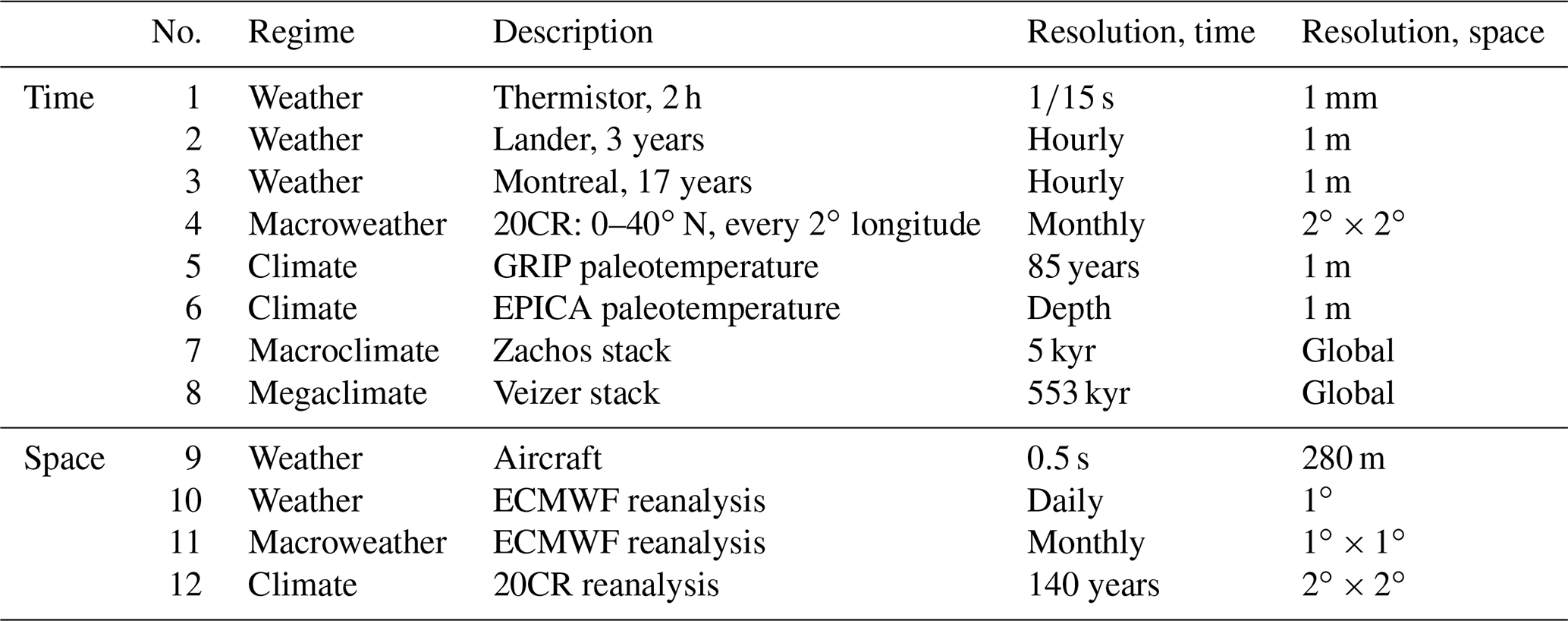
Table A2The scaling parameters H,C1, and α and the probability exponents qD. The far-right columns give theoretical estimates of the maximum spike heights using the parameters C1, α, and qD and the scale ratio λ of the plots in Fig. 2 (1000; the spike plot for data set no. 6 is not shown). The theory column uses these parameters with the multifractal theory described in the text to estimate the solution to the equation . The “observed” column determines γmax from the spike plot directly: , where is the maximum spike. For comparison, for λ=1000, Gaussian probabilities of 10−3, 10−6, and 10−9 yield respectively , 0.26, and 0.30. Error estimates for the right-hand-side columns (extremes) were not given due to their sensitivity to the somewhat subjective choice of range over which the regressions were made. Reproduced from Lovejoy (2018).
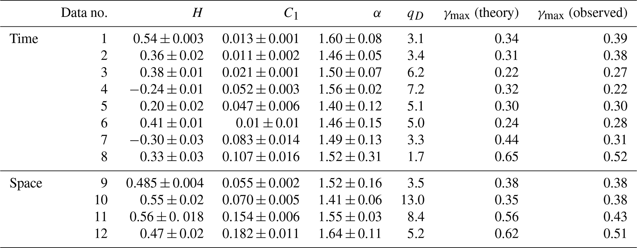
B1 Introduction
In 1994, a new H<0 data analysis technique was proposed by Peng et al. (1994) that was initially applied to biological series: the detrended fluctuation analysis (DFA) method. The key innovation was simply to first sum the series (effectively an integration of order 1), which has the effect of adding 1 to the value of H. The consequence is that, in most geophysical series and transects (as long as ), the resulting summed series had H>0, allowing the more usual difference and difference-like fluctuations to be applied. Over an interval Δt, the DFA method estimates fluctuations in the summed series by using the standard deviation of the residuals of a polynomial fit over the interval length Δt (i.e. a different regression for each fluctuation at each time interval). We return to this in more detail in Sect. B4, but for the moment, note that the interpretation of the DFA “fluctuation function” is sufficiently opaque that typical plots do not bother to even use units for the fluctuation amplitudes.
Over the following decades, there evolved several more or less independent strands of scaling analysis, each with their own mathematical formalism and interpretations. The wavelet community dealing with fluctuations directly, the DFA community wielding a method that could be conveniently implemented numerically, and the turbulence community focused on intermittency. In the meantime, most geoscientists continued to use spectral analysis, occasionally with singular spectral analysis (SSA), the multitaper method (MTM), or other refinements. New clarity was achieved by the first “Haar” wavelet (Haar, 1910). There were two reasons for this: the simplicity of its definition and calculation and the simplicity of its interpretation (Lovejoy and Schertzer, 2012). To determine the Haar fluctuation over a time interval Δt, one simply takes the average of the first half of the interval and subtracts the average of the second half (Fig. 17, bottom; see Sect. B3 for more details). As for the interpretation, when H is positive, then it is (nearly) the same as a difference, whereas whenever H is negative, the fluctuation can be interpreted as an “anomaly” (in this context an anomaly is simply the average over a segment length Δt of the series with its long-term average removed; see Sect. B3). In both cases, in addition to a useful quantification of the fluctuation amplitudes, we also recover the correct value of the exponent H. Although the Haar fluctuation is only useful for H in the range −1 to 1, this turns out to cover most of the series that are encountered in geoscience (see e.g. Fig. 18).
B2 Fluctuations revisited
The inadequacy of using differences as fluctuations forces us to use a different definition. The root of the problem is that “cancelling” series (H<0) are dominated by high frequencies, whereas “wandering” series (H>0) are dominated by low frequencies (see Figs. B3 and B4 discussed in Sect. B2). As we discuss below, differencing can be thought of as a filtering operation that de-emphasizes the low frequencies yet, in the H>1 case, it is not enough: the result depends spuriously on the very lowest frequencies present in the series (later). Conversely, the difference filter does not affect the high frequencies much, so that, in the H<0 case, difference fluctuations are spuriously determined by the very highest frequencies. In either case, the difference-filtered results are spurious in the sense that they depend on various details of the empirical samples: the overall series length and the small-scale resolution respectively. Mathematically, the link between the mean amplitude of the fluctuation and the lags has been broken.
How can we remedy the situation? First, consider the case . If we could obtain a new series whose exponent was raised by 1, then its exponent would be 1+H, which would be in the range , and hence its fluctuations could be analysed by difference fluctuations. However, this turns out to be easy to achieve. Return to the simple sinusoid, frequency ω, period : T(t)=Asin ωt, where the amplitude A of this elementary fluctuation is identified with ΔT. Now, consider its derivative: Aωcos ωt. Since the difference between sine and cosine is only a phase, taking derivatives yields oscillations/fluctuations with the same period Δt but with an amplitude multiplied by the factor . Now consider the integral : fluctuations of the series obtained by integration are simply multiplied by ω−1 or equivalently by Δt. Therefore, if the average fluctuations are scaling with 〈ΔT(Δt)〉≈ΔtH, then we expect any reasonable definition of fluctuation to have the property that fluctuations of derivatives (for discrete series, differences) or fluctuation of integrals (sums) to also be scaling but with exponents respectively decreased or increased by 1. More generally, it turns out that a filter ω−H corresponds to an Hth-order (fractional) integral (when H<0, to a (fractional) derivative).
With this in mind, consider a series with and replace it by its “running sum” so that its mean differences will have the scaling , with exponent 1+H in the useful range between zero and one. However, note now that is simply the sum of the T(t) over Δt values, and hence , where is the temporal average over the interval length Δt. We conclude that, when , the mean of a time average over an interval of length Δt has the scaling . Indeed, this provides a straightforward interpretation: when , H quantifies the rate at which the means of temporal averages decrease as the length of the temporal averaging Δt increases. The only technical detail here is that, when H<0, , so that this interpretation can only be true if the long-term (large Δt) temporal average of the series is indeed zero. To ensure this, it is sufficient to remove the overall mean of the series before taking the running sum (. Whenever , the resulting average is therefore a useful and easy-to-interpret definition of fluctuation called the “anomaly” fluctuation (this was earlier called a “tendency” fluctuation; Lovejoy and Schertzer, 2012). To distinguish it from other fluctuations, we may denote it by .
From the way it was introduced by a running-sum transformation of the series, we see that the anomaly fluctuation will be dominated by low-frequency details whenever H>0 and by high-frequency details whenever (see however Sect. B3 for some caveats when H<0). The variation of the standard deviation of the anomaly fluctuation with scale is sometimes called a “climactogram” (Koutsoyiannis and Montanari, 2007). However, because this is an anomaly statistic, it is only useful when H<0: see Lovejoy et al. (2013).
It turns out that many geophysical phenomena have both and regimes (Fig. 18), so that it is useful to have a single fluctuation definition that covers the entire range . From the preceding discussion, it might be guessed that such a definition may be obtained by combining both differencing and summing; the result is the Haar fluctuation. To obtain (ΔT(Δt))Haar, it suffices to take the differences of averages (or, equivalently, averages of differences; the order does not matter): the result is , i.e. the difference of the average over the first and second halves of the interval between t and t+Δt (note that, in terms of the running sum, s(t), this is expressed in terms of second differences). (ΔT(Δt))Haar is a useful estimate of the Δt scale fluctuation as long as . Note that we do not need to remove the overall mean , since taking differences removes any additive constant.
However, what does the Haar fluctuation mean, and how do we interpret it? Consider first the Haar fluctuation for a series with . We have seen that, for such series, the anomaly fluctuation changes little: it saturates. Therefore, taking the temporal averages of the first and second halves of the interval yields roughly the values at the centre of the intervals, so that 〈(ΔT(Δt))Haar〉=Cdiff〈(ΔT(Δt))dif〉, where Cdiff is a “calibration” constant of order 1. Conversely, consider the Haar fluctuation for a series with . In this case it is the anomaly fluctuation of the consecutive differences over intervals of length , but for H<0, the differences saturate (yielding roughly a constant independent of Δt), so that when , 〈(ΔT(Δt))Haar〉=Canom〈(ΔT(Δt))anom〉. The numerical factors Cdiff,Canom that yield the closest agreements depend on the statistics of the series. However, numerical simulations, much data analysis, and the theory discussed below show that (especially for ; see Fig. B5) using gives quite good agreement, so that if we define the “calibrated” Haar fluctuation (ΔT(Δt))Haar,cal as , then we find for and for . Therefore, the interpretation of the calibrated Haar fluctuation is very close to differences () and anomalies (), and it has the advantage of being applicable to any series with regimes in the range ; this covers almost all geophysical fields that have been analysed to date.
So what about other ranges of H, other definitions of fluctuation? From the above, the obvious method of extending the range of Hs is to use derivatives or integrals (for series, differences, and running sums) which respectively decrease or increase the exponents. Hence, for example, a fluctuation that is useful over the range can be obtained simply by taking the second difference rather than the first and combining this with summing (s(t) above) to yield the “quadratic Haar” fluctuation valid over the range : . While these higher-order fluctuations are quite adequate for estimating exponents H, the drawback is that their interpretations are no longer simple; fortunately, they are seldom needed. More examples are given in the next section.
B3 Fluctuations as convolutions, filters, and the H limits
To get a clearer idea of what is happening, let us briefly put all of this into the framework of wavelets, a very general method for defining fluctuations. The key quantity is the “mother wavelet” Ψ(t), which can be practically any function as long as it has an overall mean zero: this is the basic “admissibility condition”. The fluctuation at a scale Δt at a location t is then simply the integral of the product of the rescaled, shifted mother wavelet.
ΔT(Δt) is the Δt scale fluctuation. The fluctuations discussed in the previous section are the following special cases.
-
Difference fluctuations
-
Anomaly fluctuations
-
Haar fluctuations
These fluctuations are related by
These are shown in Fig. B1 and some other common wavelets in Fig. B2. Table B1 gives definitions and Fourier transforms.
In order to understand the convergence/divergence of different scaling processes, it is helpful to consider the Fourier transforms (indicated with a tilde). The general relation between the Fourier transform of the fluctuation at lag Δt, and the series is obtained from the fact that the fluctuation is a rescaled convolution:
We see that the fluctuation is simply a filter with respect to the original series (its Fourier transform is multiplied by ). Table B1 shows Ψ(ω) for various wavelets, and Figs. B3 and B4 show their moduli squared.
Taking the modulus squared and ensemble averaging (“〈.〉”), we obtain
where EΔT(ω) and ET(ω) are the spectra of the fluctuation and the process respectively.
We may now consider the convergence of the fluctuation variance using Parseval's theorem:
(we have used the fact that the spectrum is a symmetric function). Now consider scaling processes
and consider the high- and low-frequency dependence of the wavelet:
Plugging these forms into the integral for the fluctuation variance, we find that the latter only converges when
When H′ is outside of this range, the fluctuation variance diverges; in practice it is dominated by either the highest () or lowest () frequencies present in the sample. We use the prime since this discussion is valid for second-order moments – not only for Gaussian processes (where ), but also for multifractals where .
When , then the variance is finite and the fluctuation variance 〈ΔT(Δt)2〉 is
If ET is a pure power law (Eq. B10), then we obtain
The integral is just a constant and, since , as expected we recover the scaling of the fluctuations (). We also have C(Δt)=C as a pure “calibration” constant (independent of Δt).
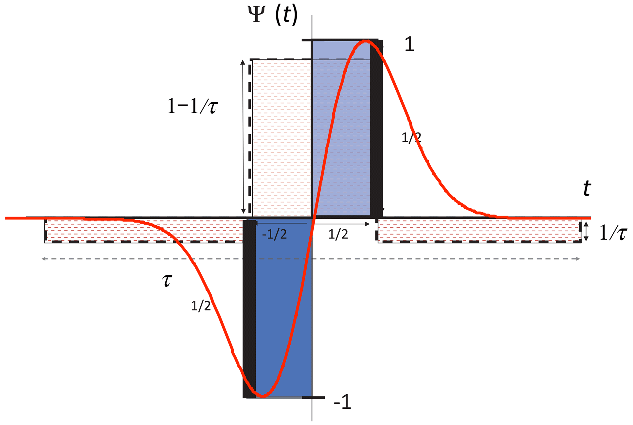
Figure B1The simpler wavelets discussed in the text: see Table A1 for mathematical definitions and properties. The black bars symbolizing Dirac delta functions (these are actually infinite in height) indicate the difference fluctuation (poor man's wavelet), the stippled red line indicates the anomaly fluctuation, the blue rectangles shows the Haar fluctuation (divided by 2), and the red line shows the first derivative of the Gaussian.
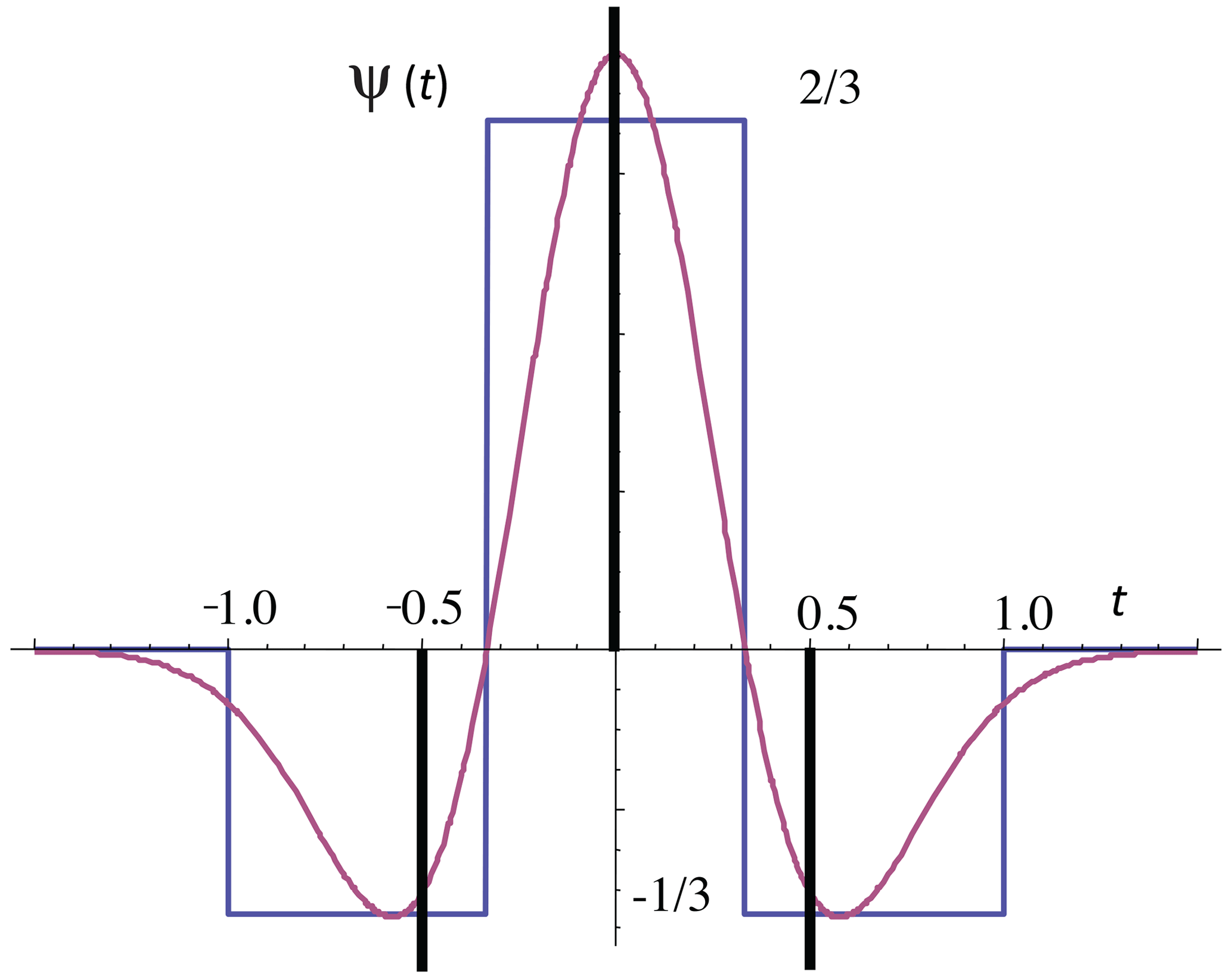
Figure B2The higher-order wavelets discussed in the text: the black bars (representing Dirac delta functions) indicate the second difference fluctuation, the solid blue the quadratic Haar fluctuation, and the red the “Mexican hat wavelet” or second derivative of the Gaussian fluctuation.
The difference between different fluctuations is the integral on the far right of Eq. (B14). As long as it converges, the difference between using two different types of fluctuations is therefore the ratio C:
where Ψref is the reference wavelet (here we consider differences or anomalies). Figure B5 shows that C for the reference wavelet equals the anomaly for and the difference for ; it can be seen that the canonical value C=2 is a compromise that is mostly accurate for but is not so bad for negative H′. If needed, we could use the theory value from the figure, but in real-world applications, there will not be perfect scaling; there may be zones of both positive and negative H′ present, so that this might not be advantageous. Finally, we defined H′ as the rms fluctuation exponent and have discussed the range over which this second-order moment converges for different wavelets characterized by Hlow, Hhigh. In the quasi-Gaussian case, we have 〈(ΔT(Δt))q〉≈ΔtqH, so that and the limits for convergence of the q=1 and q=2 moments are the same. However, more generally, in the multifractal case the limits will depend on the order of moment considered, with the range being valid for the first-order moment.
In summary, when the wavelet falls off quickly enough at high and low frequencies, the fluctuation variance converges to the expected scaling form. Conversely, whenever the inequality is not satisfied, the fluctuation variance depends spuriously on either high- or low-frequency details.
Table B1A comparison of various wavelets along with their frequency (Fourier) representation and low- and high-frequency behaviours. On the right, the range of H′ over which they are useful is indicated. For the anomaly fluctuation, see the text. The normalization for quadratic Haar is chosen to make it close to the Mexican hat.
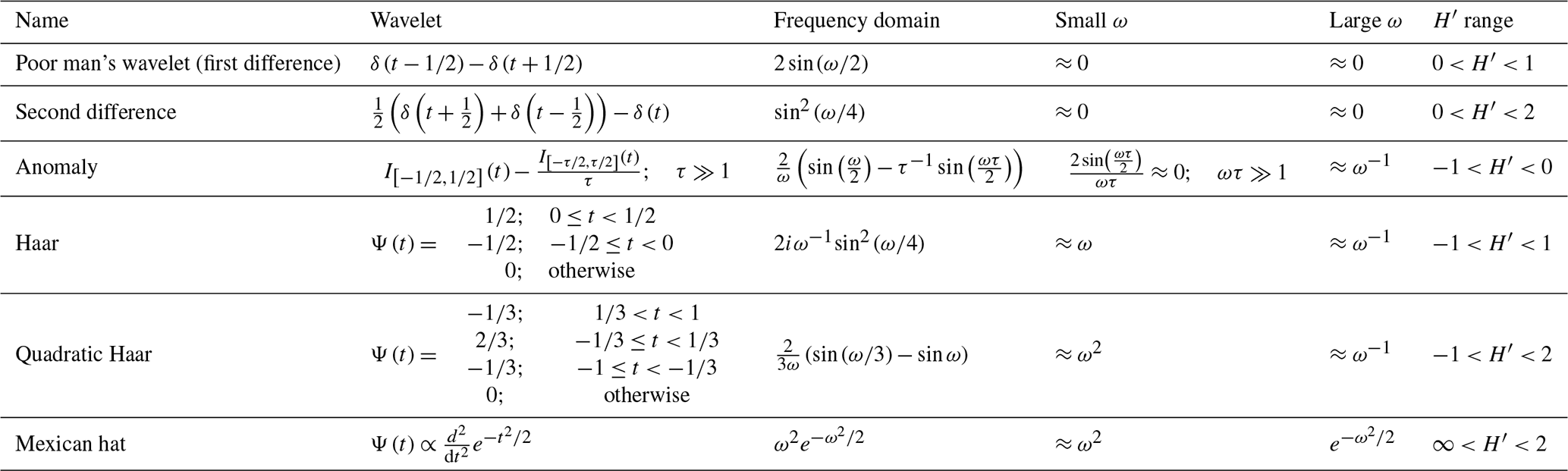
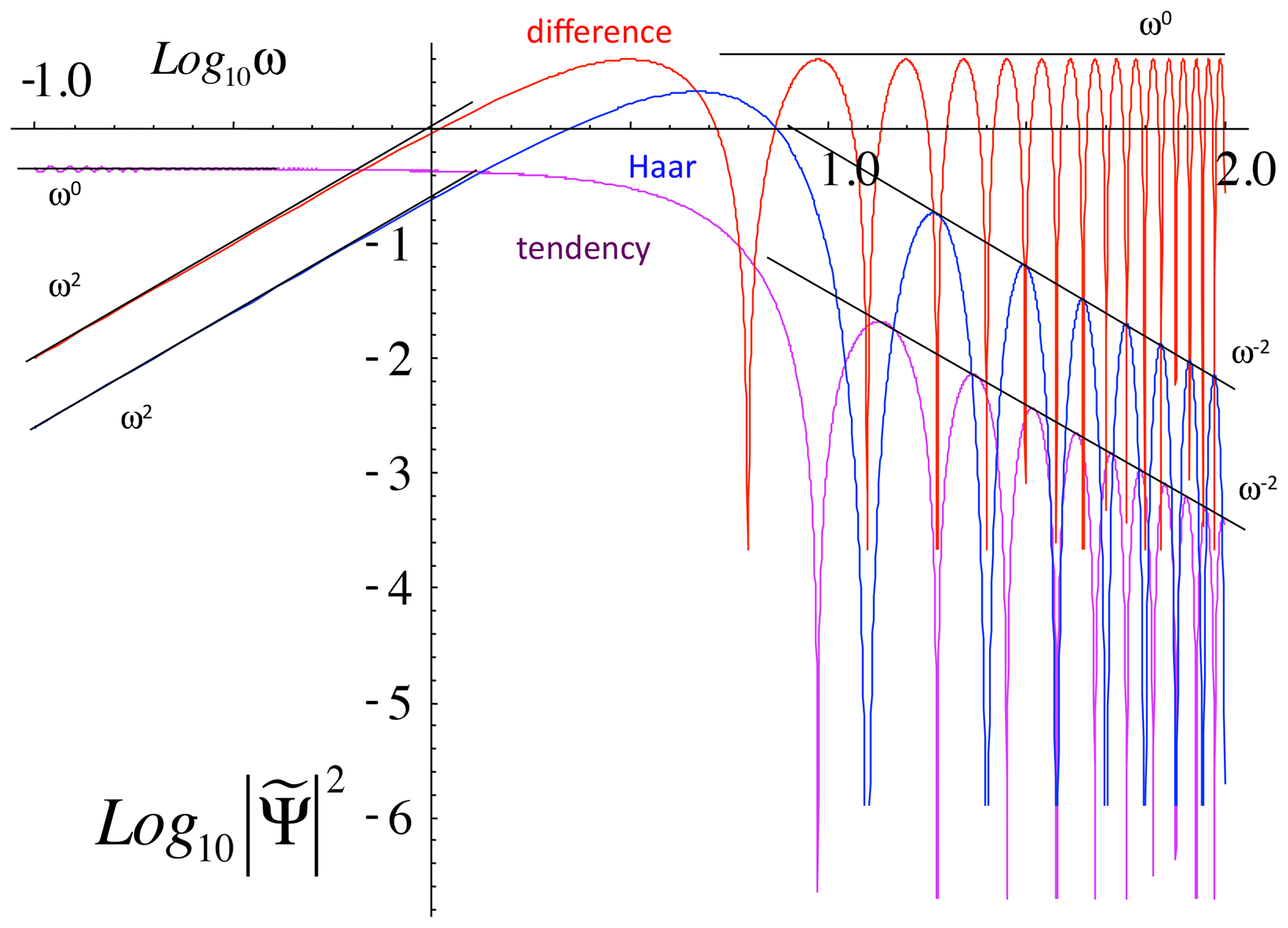
Figure B3The simple wavelets and fluctuations discussed in the text in the frequency domain. The power spectrum of the wavelet filter is shown in a log–log plot ( is the Fourier transform of Ψ(x)). The key asymptotic behaviour is shown by the reference lines.
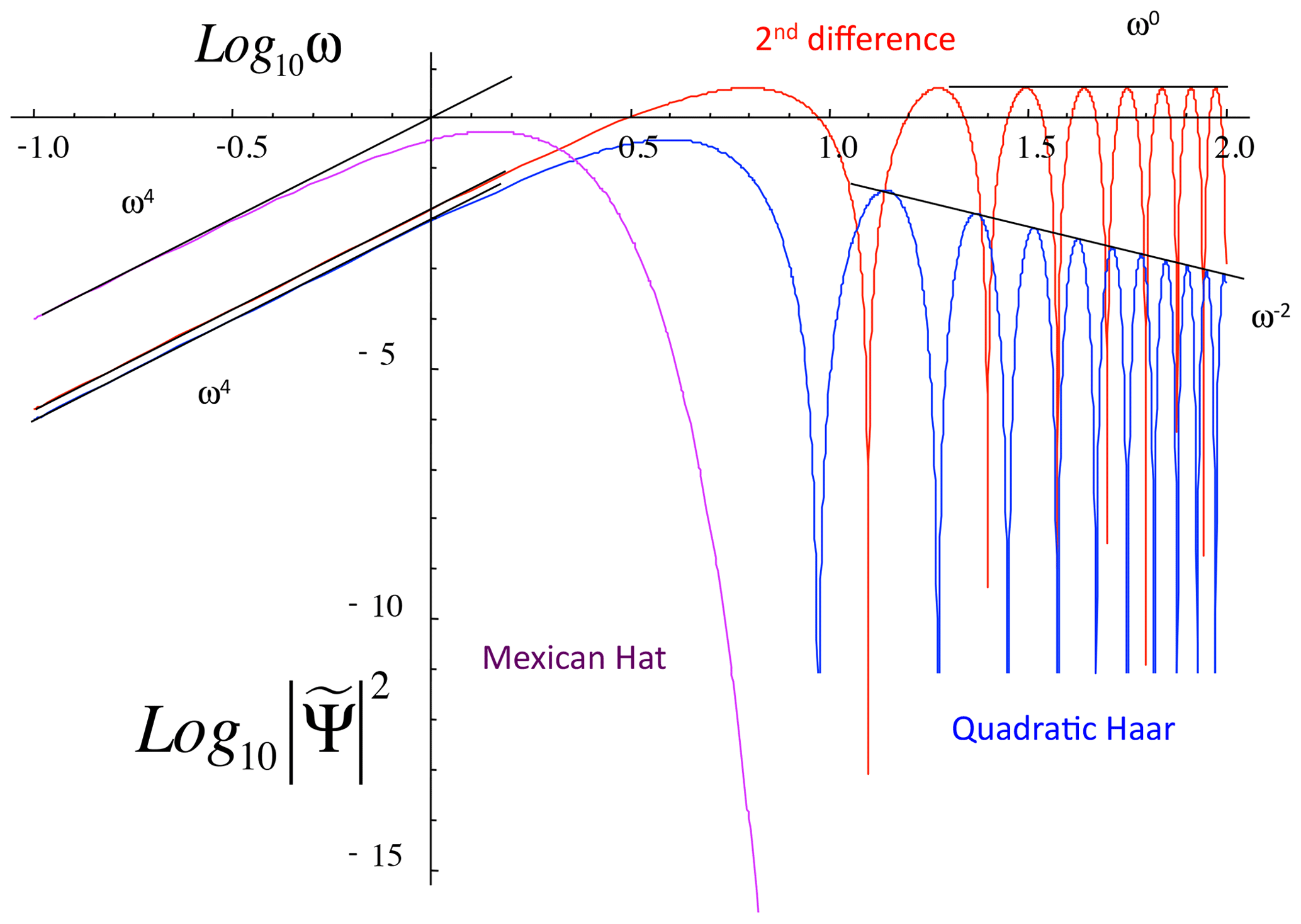
Figure B4The power-spectrum filters for the higher-order wavelets/fluctuations discussed in the text, along with reference lines indicating the asymptotic power-law behaviours. Note that the Mexican hat (second derivative of the Gaussian) decays exponentially at high frequencies, equivalent to an exponent −∞.
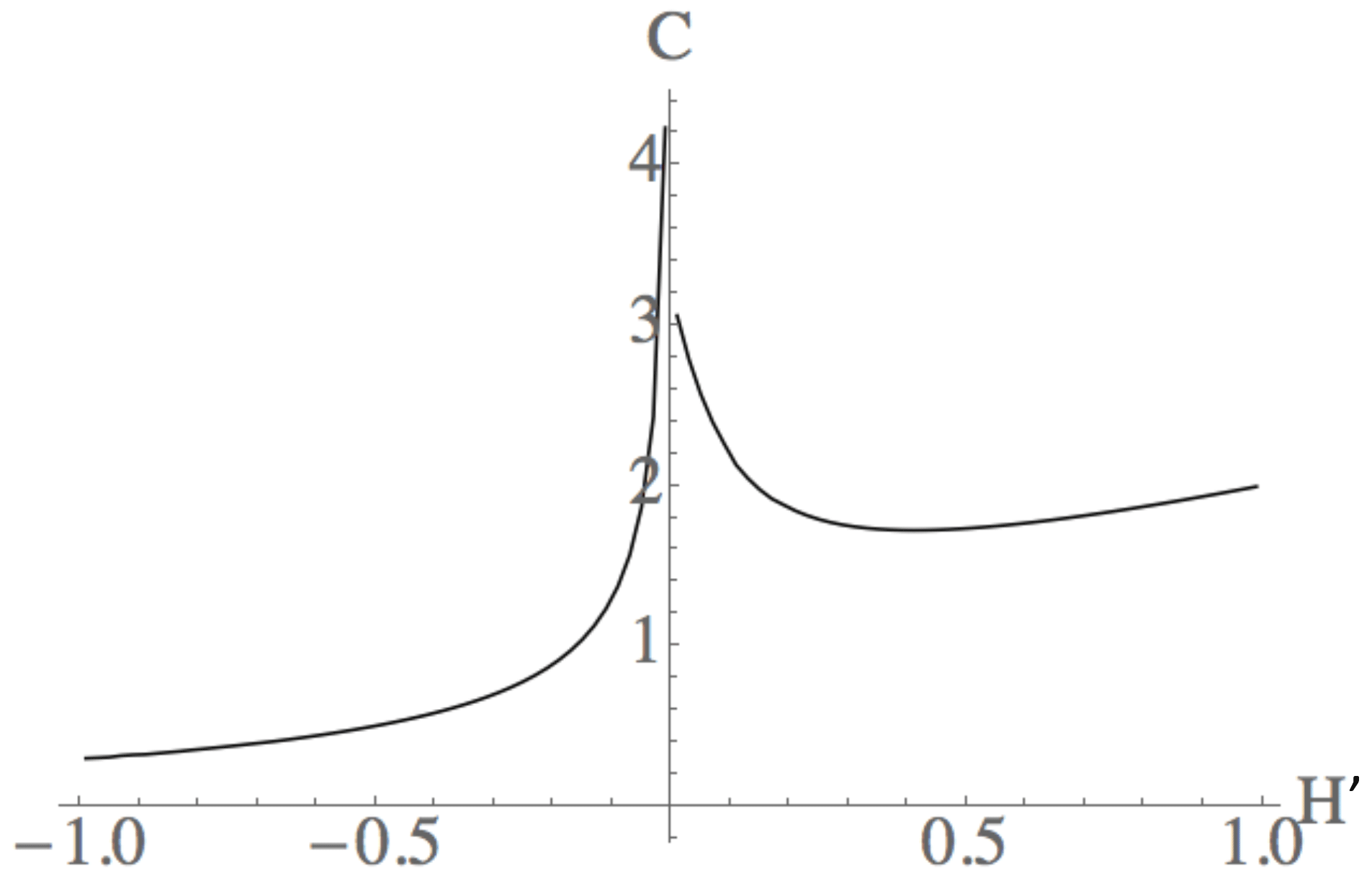
Figure B5The theoretical calibration constant C for the rms second moment (Eq. B15). Note for that it is close to the canonical value C=2.
B4 Stationarity/nonstationarity
To illustrate various issues, we made a multifractal simulation with (Fig. B6, C1=0.1, α=1.8, Sect. 3.2.2) and then took its running sum in Fig. B7. Note that, as expected, while Fig. B6 with H<0 has cancelling fluctuations, Fig. B7 with , it is wandering. Now compare the left- and right-hand sides of Fig. B7 – are they produced by the same stochastic process, or is the drift on the right-hand side caused by an external agent that was suddenly switched on? When confronted with series such as this that appear to behave differently over different intervals, it is often tempting to invoke the action of a statistically nonstationary process. This is equivalent to the conviction that no conceivable (or at least plausible) unique physical process following the same laws at all times could have produced the series. It is worth discussing stationarity in more detail since it is a frequent source of confusion: indeed, all manner of “wandering” signals lead to claims of nonstationarity. Adding to this is the fact that common stochastic processes – such as drunkard's walks (Brownian motion) – are strictly speaking nonstationary (see however below).
What is going on? The first thing to be clear about is that statistical stationarity is not a property of a series or even of a finite number of series, but rather of the stochastic process generating the series. It is a property of an infinite ensemble of series. It simply states that the statistical properties are translationally invariant along the time axis, i.e. that they do not depend on t. Statistical stationarity is simply the hypothesis that the underlying physical processes that generate the series are the same at all instants in time. In reality, the “wandering” character of an empirical signal is simply an indication that the realization of the process has low-frequency components with large amplitudes and that, over the (finite) available range, it tends to be dominated by them (this is a characteristic of all scaling processes with H>0).
However, once one assumes that the process comes from a certain theoretical framework – such as random walks – then the situation is quite different because this more specific hypothesis can be tested. However, let us take a closer look. A theoretical Brownian motion process x(t) (defined for all t≥0) is an example of a process with stationary increments: the rule for the drunk to go either to the left or to the right (an incremental change in position) is always the same, Δx(Δt) indeed independent of t. The only reason that x(t) is nonstationary is that the drunkard's starting location is special – let us say x(0)=0 – so that the statistics of x(t) depend on t. However, on any finite domain it is a trivial matter to make the process perfectly stationary: one need only randomize the drunk's starting location x(0). Note that this method does not work for purely mathematically defined Brownian motions that are defined on the infinite x axis because it is impossible to define a uniform random starting position between ±∞. However, real processes always have finite bounds and – more to the point – real scaling processes always have outer scales, so that, in practice (i.e. over finite intervals), even classical random walks can be made stationary.
B5 Non-wavelet fluctuations: detrended fluctuation analysis
We mentioned that the DFA technique was valid for (with n usually 1; linear DFA). Since it is valid for some negative H, it is an improvement over simply using differences and has been used in climate analyses (e.g. Kantelhardt et al., 2001; Koscielny-Bunde et al., 2006; Monetti et al., 2003). Unfortunately, the determination of the DFA fluctuations is not simple, nor is its interpretation, so that often the units of the fluctuation function are not even given. Other difficulties with the DFA method have been discussed in Varotsos and Efstathiou (2017).
To understand the DFA, take the running sum s(t) of the empirical time series (in DFA jargon, the “profile”; see Fig. B6). Then break s(t) into blocks of length Δt and perform regressions with nth-order polynomials (in Fig. B7, Δt was taken as half the total interval length, and linear regressions were used, i.e. n=1). For each interval length Δt, one then determines the standard deviation F of the regression residues (see Fig. B8). Since F is a fluctuation in the summed series, the DFA fluctuation in the original series (ΔT)DFA is given by
In words, (ΔT)DFA is the standard deviation of the residues of polynomial regressions on the running sums of the series divided by the interval length. Note that the usual DFA treatments do not return to the fluctuations in the original series: they analyse F (not ), which is the fluctuation of the running sum, not the original series. Due to its steeper slope (increased by 1), plots of logF-log Δt look more linear than log(-logΔt. For series with poor scaling – or with a transition between two scaling regimes – this has the effect of giving the illusion of good scaling and may have contributed to the popularity of the technique. However, in at least several instances in the literature, DFA of daily weather data (with a minimum resolution of 2 d) failed to detect the weather–macroweather transition – breaks in the scaling were spuriously hidden from view at the extremely small Δt end of the analysis.
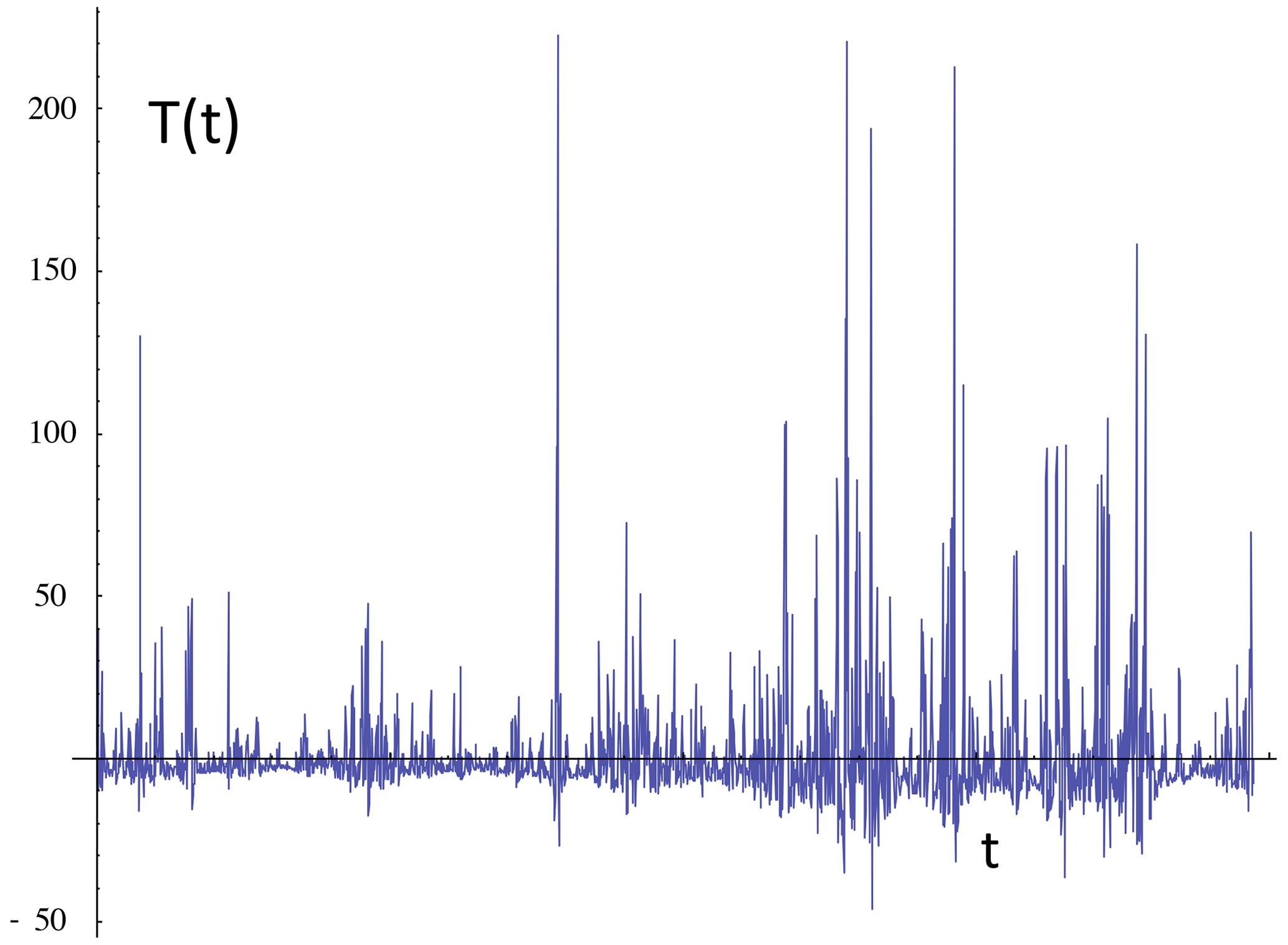
Figure B6A simulation of a (multifractal) process with , C1=0.1, and α=1.8 showing the tendency for fluctuations to cancel.
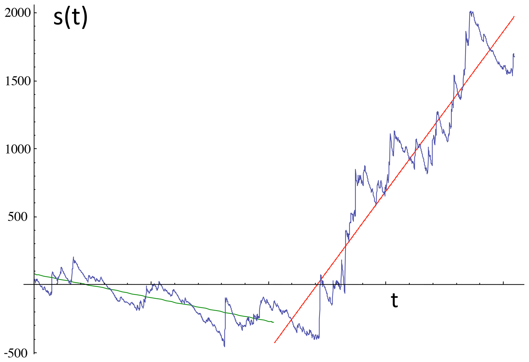
Figure B7The running sum s(t) of the previous realization with ; note the wandering character. Also shown are the two regression lines used to define the fluctuations of the detrended fluctuation analysis technique; for fluctuations with lags Δt, half of the length is shown. For each regression, the fluctuation is estimated by the rms of the residues from the lines; see Fig. B8.
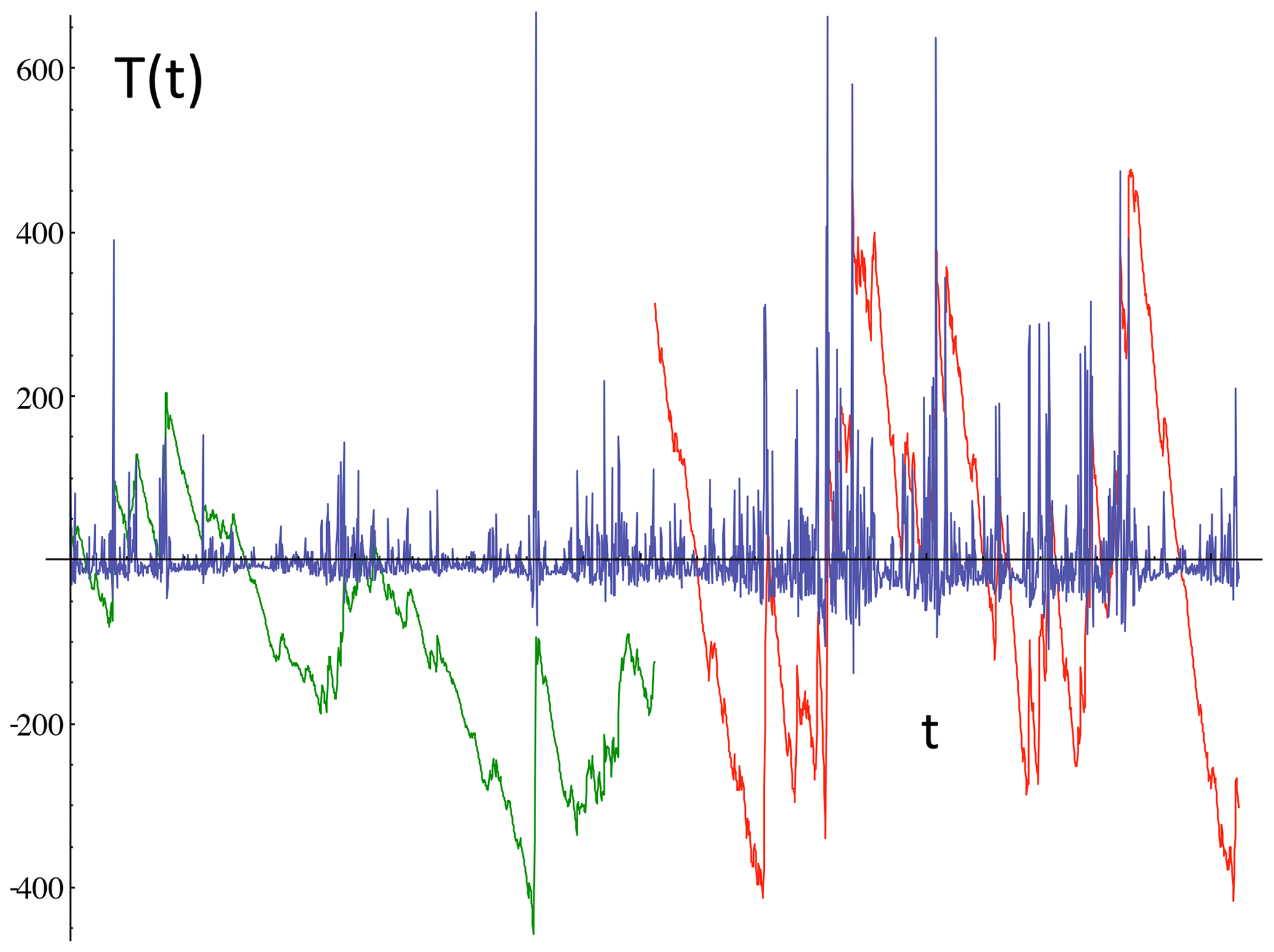
Figure B8The series of Fig. B6 with the residues of the two regression lines in Fig. B7 used to determine the DFA fluctuations for lags Δt half of the length shown (blown up by factors of 3, green and red). For each regression, the fluctuation is estimated by the rms of the residues from the lines.

Figure B9Comparison of the bias in estimates of the second-order structure function δξ(2), obtained from numerical multifractal simulations with parameters α=1.8 and C1=0.1 and with the fluctuation H as indicated. Theoretically, the (unbiased) second-order structure function exponent is , and with these parameters, K(2)=0.18. For each value of H from to (at intervals of ), 50 realizations of the process were analysed, each of length 214 = 16 384 points. Difference fluctuations were only applied to the H>0 cases and anomaly fluctuations for H<0. Spectra, Haar, and multifractal detrended fluctuation analysis (MFDFA) were applied over the whole range. We see that the latter methods are quite accurate (to within about −0.05) over the range ≈ 0.7. Over this range in particular, the Haar fluctuations have a bias of about +0.01, while the MFDFA has a bias of about −0.02. In comparison, the difference and anomaly fluctuations have stronger biases (of about ±0.1) near the limits of their ranges, i.e. when . Adapted from Lovejoy and Schertzer (2012).
Finally, the usual DFA approach defines the basic exponent a, not from the mean DFA fluctuation, but rather from the rms DFA fluctuation:
Comparing this to the previous definitions and using ΔT≈(ΔT)DFA, we see (Eq. B12) that
Interpretations of the DFA exponent a typically (and usually only implicitly) depend on the quasi-Gaussian assumption. For example, one sometimes discusses “persistence” and “antipersistence”. These behaviours can be roughly thought of as types of “cancelling” or “wandering” but with respect to Gaussian white noises (i.e. with ) rather than (as here) with respect to the mean fluctuations that are determined by the sign of H, which is equivalent to instead characterizing the scaling of the process with respect to the “conservative” (pure multiplicative, H=0) multifractal process. A “persistent” Gaussian process is one in which the successive increments are positively correlated, so that the variance of the process grows more quickly than for Brownian motion noise, i.e. , while an “antipersistent” process by contrast has successive increments that are negatively correlated, so that it grows more slowly (; see Eq. B18 with K(2)=0, which holds for Gaussian processes). For Gaussian processes this distinction is associated with precise mathematical convergence/divergence issues. However, if the process is non-Gaussian, this criterion is not relevant and the classification itself is not very helpful, whereas the sign of the fluctuation exponent H remains fundamental (in particular, in the more general multifractal case). In terms of interpretation, the drawback of the , classification is that the neutral (reference) case of persistence and antipersistence () is white noise, which itself is highly cancelling (it has ), so that, even for Gaussian processes, the persistence/antipersistence classification is not very intuitive.
In applications of the DFA method, much is said about the ability of the method to remove nonstationarities. Indeed, it is easy to see that an nth-order DFA analysis removes an nth-order polynomial in the summed series, i.e. an n−1th-order polynomial in the original series. In this, it is no different from the “Mexican hat” or other wavelets and their higher-order derivatives (or from the simple polynomial extensions of fluctuations such as the quadratic Haar fluctuation discussed above). In any case, it removes such trends at all scales, not only at the largest ones, so that it is misleading to describe it as removing nonstationarities. In addition, the stationarity assumption is still made with respect to the residuals from the polynomial regression – just as with the wavelet-based fluctuations. If one only wants to remove nonstationarities, this should be done as a “pretreatment”: i.e. trends should only be removed over the entire series and not over each interval or over each segment within the series. Finally, the most common and strongest geophysical nonstationarities are due to the diurnal and annual cycles, and none of these techniques removes oscillations.
We conclude that the only difference between analysing a data series with the DFA or with wavelet-based fluctuation definitions is the extra and needless complexity of the DFA – the regression part – that makes its interpretation and mathematical basis unnecessarily obscure. Indeed, Fig. B9 numerically compares spectra, (Haar) wavelets, and DFA exponent estimates, showing that Haar wavelets are at least as accurate as DFA but have the added advantage of simplicity of implementation and simplicity of interpretation.
If the underlying process is multifractal, one naturally obtains huge fluctuations (in space, huge structures, “singularities”), but these are totally outside the realm of quasi-Gaussian processes, so that when they are inappropriately interpreted in a quasi-Gaussian framework, they will often be mistakenly treated as nonstationarities (in space, mistakenly as inhomogeneities).
Much software is available from the site: http://www.physics.mcgill.ca/~gang/software/index.html (Lovejoy and Hébert, 2023).
This review contains no original data analyses.
The author is a member of the editorial board of Nonlinear Processes in Geophysics. The peer-review process was guided by an independent editor, and the author also has no other competing interests to declare.
Publisher's note: Copernicus Publications remains neutral with regard to jurisdictional claims in published maps and institutional affiliations.
This article is part of the special issue “Interdisciplinary perspectives on climate sciences – highlighting past and current scientific achievements”. It is not associated with a conference.
The author was helped by numerous colleagues and students over the last decades, especially Daniel Scherzter, with whom much of the multifractal and GSI material was developed. Adrian Tuck was involved in multidecadal collaborations on the subject of aircraft turbulence and scaling analyses thereof.
This paper was edited by Tommaso Alberti and reviewed by Adrian Tuck and Christian Franzke.
Adelfang, S. I.: On the relation between wind shears over various intervals, J. Appl. Meteorol., 10, 156–159, 1971.
Arias, P. A., Bellouin, N., Coppola, E., Jones, R. G., Krinner, G., Marotzke, J., Naik, V., Palmer, M. D., Plattner, G.-K., Rogelj, J., Rojas, M., Sillmann, J., Storelvmo, T., Thorne, P. W., Trewin, B., Achuta Rao, K., Adhikary, B., Allan, R. P., Armour, K., Bala, G., Barimalala, R., Berger, S., Canadell, J. G., Cassou, C., Cherchi, A., Collins, W., Collins, W. D., Connors, S. L., Corti, S., Cruz, F., Dentener, F. J., Dereczynski, C., Di Luca, A., Diongue Niang, A., Doblas-Reyes, F. J., Dosio, A., Douville, H., Engelbrecht, F., Eyring, V., Fischer, E., Forster, P., Fox-Kemper, B., Fuglestvedt, J. S., Fyfe, J. C., Gillett, N. P., Goldfarb, L., Gorodetskaya, I., Gutierrez, J. M., Hamdi, R., Hawkins, E., Hewitt, H. T., Hope, P., Islam, A. S., Jones, C., Kaufman, D. S., Kopp, R. E., Kosaka, Y., Kossin, J., Krakovska, S., Lee, J.-Y., Li, J., Mauritsen, T., Maycock, T. K., Meinshausen, M., Min, S.-K., Monteiro, P. M. S., Ngo-Duc, T., Otto, F., Pinto, I., Pirani, A. Raghavan, K., Ranasinghe, R., Ruane, A. C., Ruiz, L., Sallée, J.-B., Samset, B. H., Sathyendranath, S., Seneviratne, S. I., Sörensson, A. A., Szopa, S., Takayabu, I., Tréguier, A.-M., van den Hurk, B., Vautard, R., von Schuckmann, K., Zaehle, S., Zhang, X., and Zickfeld, K.: Climate Change 2021: The Physical Science Basis. Contribution of Working Group I to the Sixth Assessment Report of the Intergovernmental Panel on Climate Change, Cambridge, United Kingdom and New York, NY, USA, Cambridge University Press, https://doi.org/10.1017/9781009157896.002, 2021.
Ashkenazy, Y., Baker, D., Gildor, H., and Havlin, S.: Nonlinearity and multifractality of climate change in the past 420,000 years, Geophys. Res. Lett., 30, 2146 https://doi.org/10.1029/2003GL018099, 2003.
Bak, P., Tang, C., and Weiessenfeld, K.: Self-Organized Criticality: An explanation of 1/f noise, Phys. Rev. Lett., 59, 381–384, 1987.
Batchelor, G. K. and Townsend, A. A.: The Nature of turbulent motion at large wavenumbers, P. Roy. Soc. Lond. A, A199, 208—256, 1949.
Blender, R., Fraedrich, K., and Hunt, B.: Millennial climate variability: GCM-simulation and Greenland ice cores, Geophys. Res. Lett., 33, L04710, https://doi.org/10.1029/2005GL024919, 2006.
Blöschl, G., Thybo, H., Savenije, H., and Lovejoy, S.: Introduction, in: A voyage through scales: The Earth System in Space and Time, edited by: Blöschl, G., Thybo, H., and Savenije, H., Edition Lammerhuber, 13–18, ISBN 978-3-901753-84-8, 2015.
Boeke, K.: Cosmic View: The Universe in Forty Jumps, John Day, ISBN-10 0381980162, ISBN-13 978-0381980160, 1957.
Bolgiano, R.: Turbulent spectra in a stably stratified atmosphere, J. Geophys. Res., 64, 2226–2232, 1959.
Bunde, A., Eichner, J. F., Havlin, S., Koscielny-Bunde, E., Schellnhuber, H. J., and Vyushin, D.: Comment on “Scaling of Atmosphere and Ocean Temperature Correlations in observations and Climate Models”, Phys. Rev. Lett., 92, p039801-1-039801-5, 2004.
Charney, J. G.: Geostrophic Turbulence, J. Atmos. Sci., 28, 1087–1101, 1971.
Chen, W., Lovejoy, S., and Muller, J. P.: Mars' atmosphere: the sister planet, our statistical twin, J. Geophys. Res.-Atmos., 121, 11968–11988, https://doi.org/10.1002/2016JD025211, 2016.
Chigirinskaya, Y., Schertzer, D., Lovejoy, S., Lazarev, A., and Ordanovich, A.: Unified multifractal atmospheric dynamics tested in the tropics: part I, horizontal scaling and self criticality, Nonlin. Processes Geophys., 1, 105–114, https://doi.org/10.5194/npg-1-105-1994, 1994.
Chigirinskaya, Y., Schertzer, D., Salvadori, G., Ratti, S., and Lovejoy, S.: Chernobyl 137Cs cumulative soil deposition in Europe: is it multifractal?, in: Chaos, Fractals and models 96, edited by: Guindani, F. M. and Salvadori, G., Italian University Press, 65–72, 1998.
Corrsin, S.: On the spectrum of Isotropic Temperature Fluctuations in an isotropic Turbulence, J. Appl. Phys., 22, 469–473, 1951.
De Lima, I.: Multifractals and the temporal structure of rainfall, phD thesis, Wageningen Agricultural University, Wageningen, The Netherlands, 225 pp., 1998.
De Lima, I. and Grasman, J., Multifractal analysis of 15-min and daily rainfall from a semi-arid region in Portugal, J. Hydrol., 220, 1–11, 1999.
de Lima, M. I. P. and Lovejoy, S.: Macroweather precipitation variability up to global and centennial scales, Water Resour. Res., 51, 9490–9513, https://doi.org/10.1002/2015WR017455, 2015.
Del Rio Amador, L. and Lovejoy, S.: Predicting the global temperature with the Stochastic Seasonal to Interannual Prediction System (StocSIPS), Clim. Dynam., 53, 4373–4411, https://doi.org/10.1007/s00382-019-04791-4, 2019.
Del Rio Amador, L. and Lovejoy, S.: Long-range Forecasting as a Past Value Problem: Untangling Correlations and Causality with scaling, Geophys. Res. Lett., 48, e2020GL092147, https://doi.org/10.1029/2020GL092147, 2021a.
Del Rio Amador, L. and Lovejoy, S.: Using regional scaling for temperature forecasts with the Stochastic Seasonal to Interannual Prediction System (StocSIPS), Clim. Dynam., 57, 727–756, https://doi.org/10.1007/s00382-021-05737-5, 2021b.
de Montera, L., Barthès, L., Mallet, C., and Golé, P.: Rain universal multifractal parameters revisited with Dual-Beam Spectropluviometer measurements, J. Hydrometeorol., 10, 493–506, 2009.
Dijkstra, H.: Nonlinear Climate Dynamics, Cambridge University Press, 357 pp., ISBN 9781139034135, 2013.
Ditlevsen, P. D.: Observation of alpha-stable noise induced millennial climate changes from an ice-core record, Geophys. Res. Lett., 26, 1441–1444, 1999.
Ditlevsen, P. D., Svensmark, H., and Johson, S.: Contrasting atmospheric and climate dynamics of the last-glacial and Holocene periods, Nature, 379, 810–812, 1996.
Eichner, J. F., Koscielny-Bunde, E., Bunde, A., Havlin, S., and Schellnhuber, H.-J.: Power-law persistance and trends in the atmosphere: A detailed studey of long temperature records, Phys. Rev. E, 68, 046133, https://doi.org/10.1103/PhysRevE.68.046133, 2003.
Endlich, R. M., Singleton, R. C., and Kaufman, J. W.: Spectral Analyes of detailed vertical wind profiles, J. Atmos. Sci., 26, 1030–1041, 1969.
Feller, W.: An Introduction to probability theory and its applications, Vol. 2, Wiley, 669 pp., ISBN 978-0-471-25709-7, 1971.
Fjortoft, R.: On the changes in the spectral distribution of kinetic energy in two dimensional, nondivergent flow, Tellus, 7, 168–176, 1953.
Fraedrich, K., Blender, R., and Zhu, X.: Continuum Climate Variability: Long-Term Memory, Scaling, and 1/f-Noise, Int. J. Modern Phys. B, 23, 5403–5416, 2009.
Franzke, C.: Long-range dependence and climate noise characteristics of Antarctica temperature data, J. Climate, 23, 6074–6081, https://doi.org/10.1175/2010JCL13654.1, 2010.
Franzke, C.: Nonlinear trends, long-range dependence and climate noise properties of temperature, J. Climate, 25, 4172–4183 https://doi.org/10.1175/JCLI-D-11-00293.1, 2012.
Frisch, U., Sulem, P. L., and Nelkin, M.: A simple dynamical model of intermittency in fully develop turbulence, J. Fluid Mech., 87, 719–724, 1978.
Gagnon, J.-S., Lovejoy, S., and Schertzer, D.: Multifractal earth topography, Nonlin. Processes Geophys., 13, 541–570, https://doi.org/10.5194/npg-13-541-2006, 2006.
Garcia-Marin, A. P., Jimenez-Hornero, F. J., and Ayuso-Munoz, J. L.: Universal multifractal description of an hourly rainfall time series from a location in southern Spain, Atmosfera, 21, 347–355, 2008.
Ghil, M.: Natural climate variability, in: Encyclopedia of Global Environmental Change, Vol. 1, edited by: Munn, M. M. T. E. and Perry, J., J. Wiley & Sons, 544–549, ISBN 978-0-471-97796-4, 2002.
Ghil, M. and Lucarini, V.: The physics of climate variability and climate change, Rev. Modern Phys., 92, 035002, https://doi.org/10.1103/RevModPhys.92.035002, 2020.
Grassberger, P. and Procaccia, I.: Measuring the strangeness of Strange atractors, Physica D, 9, 189–208, 1983.
Grossman, E. L. and Joachimski, M. M.: Ocean temperatures through the Phanerozoic reassessed, Sci. Rep., 12, 8938, https://doi.org/10.1038/s41598-022-11493-1, 2022.
Guillaume, A., Kahn, B. H., Yue, Q., Fetzer, E. J., Wong, S., Manipon, G. J., Hua, H., and Wilson, B. D.: Horizontal And Vertical Scaling Of Cloud Geometry Inferred From Cloudsat Data, J. Atmos. Sci., 75, 2187–2197, https://doi.org/10.1175/jas-d-17-0111.1, 2018.
Haar, A.: Zur Theorie des orthogonalen Funktionsysteme, Math. Ann., 69, 331–371, 1910.
Halsey, T. C., Jensen, M. H., Kadanoff, L. P., Procaccia, I., and Shraiman, B.: Fractal measures and their singularities: the characterization of strange sets, Phys. Rev. A, 33, 1141–1151, 1986.
Harris, D., Menabde, M., Seed, A., and Austin, G.: Multifractal characterizastion of rain fields with a strong orographics influence, J. Geophys. Res., 101, 26405–26414, 1996.
Hébert, R., Rehfeld, K., and Laepple, T.: Comparing estimation techniques for temporal scaling in palaeoclimate time series, Nonlin. Processes Geophys., 28, 311–328, https://doi.org/10.5194/npg-28-311-2021, 2021a.
Hébert, R., Lovejoy, S., and Tremblay, B.: An Observation-based Scaling Model for Climate Sensitivity Estimates and Global Projections to 2100, Clim. Dynam., 56, 1105–1129 https://doi.org/10.1007/s00382-020-05521-x, 2021b.
Hentschel, H. G. E. and Procaccia, I.: The infinite number of generalized dimensions of fractals and strange attractors, Physica D, 8, 435–444, 1983.
Hovde, S. J., Tuck, A. F., Lovejoy, S., and Schertzer, D.: Vertical scaling of temperature, wind and humidity fluctuations: dropsondes from 13 km to the surface of the Pacific Ocean, Int. J. Remote Sens., 32, 5891–5918, https://doi.org/10.1080/01431161.2011.602652, 2011.
Hubert, P., Biaou, A., and Schertzer, D.: De la Meso-Echelle à la Micro-Echelle: Desagregation/Agregation Multifractale et Spatio-Temporelle des Precipitations. Rep., Report, Armines-EdF, 2002.
Hubert, P., Tessier, Y., Ladoy, P., Lovejoy, S., Schertzer, D., Carbonnel, J. P., Violette, S., Desurosne, I., and Schmitt, F.: Multifractals and extreme rainfall events, Geophys. Res. Lett., 20, 931–934, 1993.
Hurst, H. E.: Long-term storage capacity of reservoirs, T. Am. Soc. Civil Eng., 116, 770–808, 1951.
Huybers, P., and Curry, W.: Links between annual, Milankovitch and continuum temperature variability, Nature, 441, 329–332, https://doi.org/10.1038/nature04745, 2006.
Kadau, K., Barber, J. L., Germann, T. C., Holian, B. L., and Alder, B. J.: Atomistic methods in fluid simulation, Philos. T. Roy. Soc. A, 368, 1547–1560, https://doi.org/10.1098/rsta.2009.0218, 2010.
Kantelhardt, J. W., Koscielny-Bunde, E., Rego, H. H. A., Havlin, S., and Bunde, S.: Detecting long range corelations with detrended flucutation analysis, Physica A, 295, 441–454, 2001.
Karman, T. and Howarth, L.: On the statistical theory of isotropic turbulence, P. Roy. Soc. Lond. A, 164, 192–215, 1938.
Kiely, G. and Ivanova, K.: Multifractal analysis of hourly precipitation, Phys. Chem. Earth B, 24, 781–786, 1999.
Kolmogorov, A. N.: Local structure of turbulence in an incompressible liquid for very large Reynolds numbers (English translation: Proc. Roy. Soc. A434, 9–17, 1991), Proc. Acad. Sci. URSS., Geochem. Sect., 30, 299–303, 1941.
Kolmogorov, A. N.: A refinement of previous hypotheses concerning the local structure of turbulence in viscous incompressible fluid at high Reynolds number, J. Fluid Mech., 83, 349–369, 1962.
Koscielny-Bunde, E., Kantelhardt, J. W., Braund, P., Bunde, A., and Havlin, S.: Long-term persistence and multifractality of river runoff records: Detrended fluctuation studies, J. Hydrol. 322, 120–137, 2006.
Koscielny-Bunde, E., Bunde, A., Havlin, S., Roman, H. E., Goldreich, Y., and Schellnhuber, H. J.: Indication of a universal persistence law governing atmospheric variability, Phys. Rev. Lett., 81, 729–732, 1998.
Koutsoyiannis, D. and Montanari, A.: Statistical analysis of hydroclimatic time series: Uncertainty and insights, Water Resour. Res., 43, W05429, https://doi.org/10.1029/2006wr005592, 2007.
Kraichnan, R. H.: Inertial ranges in two-dimensional turbulence, Phys. Fluids, 10, 1417–1423, 1967.
Lacorta, G., Aurell, E., Legras, B., and Vulpiani, A.: Evidence for a k spectrum from the EOLE Lagrangian balloons in the lower stratosphere, J. Atmos. Sci., 61, 2936–2942, 2004.
Ladoy, P., Lovejoy, S., and Schertzer, D.: Extreme Variability of climatological data: Scaling and Intermittency, in: Non-linear variability in geophysics: Scaling and Fractals, edited by: Schertzer, D. and Lovejoy, S., Kluwer, 241–250, ISBN-13 978-0792309857, 1991.
Ladoy, P., Schmitt, F., Schertzer, D., and Lovejoy, S.: Variabilité temporelle des observations pluviométriques à Nimes, CR Acad. Sci. II, 317, 775–782, 1993.
Laliberté, F., Zika, J., Mudryk, L., Kushner, P. J., Kjellsson, J., and Döös, K.: Constrained work output of the moist atmospheric heat engine in a warming climate, Science, 347, 540–543, https://doi.org/10.1126/science.1257103, 2015.
Landais, F., Schmidt, F., and Lovejoy, S.: Universal multifractal Martian topography, Nonlin. Processes Geophys., 22, 713–722, https://doi.org/10.5194/npg-22-713-2015, 2015.
Lanfredi, M., Simoniello, T., Cuomo, V., and Macchiato, M.: Discriminating low frequency components from long range persistent fluctuations in daily atmospheric temperature variability, Atmos. Chem. Phys., 9, 4537–4544, https://doi.org/10.5194/acp-9-4537-2009, 2009.
Lavallée, D., Lovejoy, S., and Schertzer, D.: On the determination of the codimension function, in: Non-linear variability in geophysics: Scaling and Fractals, edited by: Schertzer, D. and Lovejoy, S., Kluwer, 99–110, ISBN-13 978-0792309857, 1991.
Lavallée, D., Lovejoy, S., Schertzer, D., and Ladoy, P.: Nonlinear variability and landscape topography: analysis and simulation, in: Fractals in geography, edited by: De Cola, L. and Lam, N., Prentice-Hall, 171–205, ISBN-10 1930665695, 1993.
Lazarev, A., Schertzer, D., Lovejoy, S., and Chigirinskaya, Y.: Unified multifractal atmospheric dynamics tested in the tropics: part II, vertical scaling and generalized scale invariance, Nonlin. Processes Geophys., 1, 115–123, https://doi.org/10.5194/npg-1-115-1994, 1994.
Lennartz, S. and Bunde, A.: Trend evaluation in records with long term memory: Application to global warming, Geophys. Res. Lett., 36, L16706, https://doi.org/10.1029/2009GL039516, 2009.
Lesieur, M.: Turbulence in fluids, Martinus Nijhoff Publishers, ISBN 9781402064340, 1987.
Lilley, M., Lovejoy, S., Strawbridge, K., and Schertzer, D.: 23/9 dimensional anisotropic scaling of passive admixtures using lidar aerosol data, Phys. Rev. E, 70, 036307-036301-036307, 2004.
Lorenz, E. N.: The predictability of a flow which possesses many scales of motion, Tellus, 21, 289–307, 1969.
Lovejoy, S.: Area perimeter relations for rain and cloud areas, Science, 187, 1035–1037, 1982.
Lovejoy, S.: What is climate?, EOS, 94, 1–2, 2013.
Lovejoy, S.: Scaling fluctuation analysis and statistical hypothesis testing of anthropogenic warming, Clim. Dynam., 42, 2339–2351, https://doi.org/10.1007/s00382-014-2128-2, 2014.
Lovejoy, S.: A voyage through scales, a missing quadrillion and why the climate is not what you expect, Clim. Dynam., 44, 3187–3210 https://doi.org/10.1007/s00382-014-2324-0, 2015.
Lovejoy, S.: How accurately do we know the temperature of the surface of the earth?, Clim. Dynam., 49, 4089–4106, https://doi.org/10.1007/s00382-017-3561-9, 2017a.
Lovejoy, S.: How scaling fluctuation analysis transforms our view of the climate, PAGES Mag., 25, 136–137, https://doi.org/10.22498/pages.25.3.136, 2017b.
Lovejoy, S.: The spectra, intermittency and extremes of weather, macroweather and climate, Nat. Sci. Rep., 8, 1–13, https://doi.org/10.1038/s41598-018-30829-4, 2018.
Lovejoy, S.: Weather, Macroweather and Climate: our random yet predictable atmosphere, Oxford University Press, 334 pp., ISBN 978-0-19-086421-7, 2019.
Lovejoy, S.: The half-order energy balance equation – Part 2: The inhomogeneous HEBE and 2D energy balance models, Earth Syst. Dynam., 12, 489–511, https://doi.org/10.5194/esd-12-489-2021, 2021a.
Lovejoy, S.: The half-order energy balance equation – Part 1: The homogeneous HEBE and long memories, Earth Syst. Dynam., 12, 469–487, https://doi.org/10.5194/esd-12-469-2021, 2021b.
Lovejoy, S.: The future of climate modelling: Weather Details, Macroweather stochastics – or both?, Meteorology, 1, 414–449, https://doi.org/10.3390/meteorology1040027, 2022a.
Lovejoy, S.: Scaling and Scale Invariance, in Encyclopedia of Mathematical Geosciences, edited by: Daya Sagar, B. S., Cheng, Q., McKinley, J., and Agterberg, F., Springer International Publishing, 1–13, ISBN 978-3-030-26050-7, 2022b.
Lovejoy, S.: Fractional relaxation noises, motions and the fractional energy balance equation, Nonlin. Processes Geophys., 29, 93–121, https://doi.org/10.5194/npg-29-93-2022, 2022c.
Lovejoy, S. and Hébert, R.: Multifractal Analysis Functions, 2010–present available in Mathematica and Matlab [code], http://www.physics.mcgill.ca/~gang/software/index.html, last access: 14 July 2023.
Lovejoy, S. and Lambert, F.: Spiky fluctuations and scaling in high-resolution EPICA ice core dust fluxes, Clim. Past, 15, 1999–2017, https://doi.org/10.5194/cp-15-1999-2019, 2019.
Lovejoy, S. and Mandelbrot, B. B.: Fractal properties of rain and a fractal model, Tellus A, 37, 209–221, 1985.
Lovejoy, S. and Schertzer, D.: Scale invariance in climatological temperatures and the spectral plateau, Ann. Geophys., 4B, 401–410, 1986a.
Lovejoy, S. and Schertzer, D.: Scale invariance in climatological temperatures and the local spectral plateau, Ann. Geophys., 4B, 401–410, 1986b.
Lovejoy, S. and Schertzer, D.: Scaling and multifractal fields in the solid earth and topography, Nonlin. Processes Geophys., 14, 465–502, https://doi.org/10.5194/npg-14-465-2007, 2007a.
Lovejoy, S. and Schertzer, D.: Scale, scaling and multifractals in geophysics: twenty years on, in: Nonlinear dynamics in geophysics, edited by: Tsonis, J. E. A. A., Elsevier, 311–337, 2007b.
Lovejoy, S. and Schertzer, D.: Scale, scaling and multifractals in geophysics: twenty years on, in: Nonlinear dynamics in geophysics, edited by: Tsonis, J. E. A. A., Elsevier, 311–337, ISBN-13 978-0387349176, 2007c.
Lovejoy, S. and Schertzer, D.: On the simulation of continuous in scale universal multifractals, part II: space-time processes and finite size corrections, Comput. Geosci., 36, 1404–1413, https://doi.org/10.1016/j.cageo.2010.07.001, 2010a.
Lovejoy, S. and Schertzer, D.: On the simulation of continuous in scale universal multifractals, part I: spatially continuous processes, Comput. Geosci., 36, 1393–1403, https://doi.org/10.1016/j.cageo.2010.04.010, 2010b.
Lovejoy, S. and Schertzer, D.: Towards a new synthesis for atmospheric dynamics: space-time cascades, Atmos. Res., 96, 1–52, https://doi.org/10.1016/j.atmosres.2010.01.004, 2010c.
Lovejoy, S. and Schertzer, D.: Space-time cascades and the scaling of ECMWF reanalyses: fluxes and fields, J. Geophys. Res., 116, D14117, https://doi.org/10.1029/2011JD015654, 2011.
Lovejoy, S. and Schertzer, D.: Haar wavelets, fluctuations and structure functions: convenient choices for geophysics, Nonlin. Processes Geophys., 19, 513–527, https://doi.org/10.5194/npg-19-513-2012, 2012a.
Lovejoy, S. and Schertzer, D.: Low frequency weather and the emergence of the Climate, in: Extreme Events and Natural Hazards: The Complexity Perspective, edited by: Sharma, A. S., Bunde, A., Baker, D. N., and Dimri, V. P., AGU monographs, 231–254, ISBN 978-0-87590-486-3, 2012b.
Lovejoy, S. and Schertzer, D.: The Weather and Climate: Emergent Laws and Multifractal Cascades, Cambridge University Press, 496 pp., ISBN 978-1-107-01898-3, 2013.
Lovejoy, S. and Spiridonov, A.: The Fractional Macroevolution Model, a simple quantitative macroevolution model, Paleobiology, in review, 2023.
Lovejoy, S., Schertzer, D., and Ladoy, P.: Fractal characterisation of inhomogeneous measuring networks, Nature, 319, 43–44, 1986.
Lovejoy, S., Schertzer, D., and Tsonis, A. A.: Functional Box-Counting and Multiple Elliptical Dimensions in rain, Science, 235, 1036–1038, 1987.
Lovejoy, S., Currie, W. J. C., Tessier, Y., Claeredeboudt, M., Roff, J., Bourget, E., and Schertzer, D.: Universal Multifractals and Ocean patchiness Phytoplankton, physical fields and coastal heterogeneity, J. Plankton Res., 23, 117–141, 2001.
Lovejoy, S., Schertzer, D., and Gagnon, J. S.: Multifractal simulations of the Earth's surface and interior: anisotropic singularities and morphology, in GIS and Spatial Analysis, Proc. Inter. Assoc. Math. Geology, edited by: Cheng, G. B.-C. Q., 37–54, 2005.
Lovejoy, S., Tuck, A. F., Hovde, S. J., and Schertzer, D.: Is isotropic turbulence relevant in the atmosphere?, Geophys. Res. Lett., 34, L14802, https://doi.org/10.1029/2007GL029359, 2007.
Lovejoy, S., Schertzer, D., and Allaire, V.: The remarkable wide range scaling of TRMM precipitation, Atmos. Res., 90, 10–32, https://doi.org/10.1016/j.atmosres.2008.02.016, 2008a.
Lovejoy, S., Schertzer, D., Lilley, M., Strawbridge, K. B., and Radkevitch, A.: Scaling turbulent atmospheric stratification, Part I: turbulence and waves, Q. J. Roy. Meteor. Soc., 134, 277–300 https://doi.org/10.1002/qj.201, 2008b.
Lovejoy, S., Tuck, A. F., Hovde, S. J., and Schertzer, D.: The vertical cascade structure of the atmosphere and multifractal drop sonde outages, J. Geophy. Res., 114, D07111, https://doi.org/10.1029/2008JD010651, 2009a.
Lovejoy, S., Tuck, A. F., Schertzer, D., and Hovde, S. J.: Reinterpreting aircraft measurements in anisotropic scaling turbulence, Atmos. Chem. Phys., 9, 5007–5025, https://doi.org/10.5194/acp-9-5007-2009, 2009b.
Lovejoy, S., Tuck, A. F., Schertzer, D., and Hovde, S. J.: Reinterpreting aircraft measurements in anisotropic scaling turbulence, Atmos. Chem. Phys., 9, 5007–5025, https://doi.org/10.5194/acp-9-5007-2009, 2009c.
Lovejoy, S., Watson, B., Grosdidier, Y., and Schertzer, D.: Scattering in Thick Multifractal Clouds, Part II: Multiple Scattering, Physica A, 388, 3711–3727, https://doi.org/10.1016/j.physa.2009.05.037, 2009d.
Lovejoy, S., Schertzer, D., Allaire, V., Bourgeois, T., King, S., Pinel, J., and Stolle, J.: Atmospheric complexity or scale by scale simplicity?, Geophys. Res. Lett., 36, L01801 https://doi.org/10.1029/2008GL035863, 2009e.
Lovejoy, S., Tuck, A. F., and Schertzer, D.: The Horizontal cascade structure of atmospheric fields determined from aircraft data, J. Geophys. Res., 115, D13105, https://doi.org/10.1029/2009JD013353, 2010.
Lovejoy, S., Schertzer, D., and Varon, D.: Do GCMs predict the climate ... or macroweather?, Earth Syst. Dynam., 4, 439–454, https://doi.org/10.5194/esd-4-439-2013, 2013.
Lovejoy, S., Muller, J. P., and Boisvert, J. P.: On Mars too, expect macroweather, Geophys. Res. Lett., 41, 7694–7700, https://doi.org/10.1002/2014GL061861, 2014.
Lovejoy, S., del Rio Amador, L., and Hébert, R.: The ScaLIng Macroweather Model (SLIMM): using scaling to forecast global-scale macroweather from months to decades, Earth Syst. Dynam., 6, 637–658, https://doi.org/10.5194/esd-6-637-2015, 2015.
Lovejoy, S., Procyk, R., Hébert, R., and del Rio Amador, L.: The Fractional Energy Balance Equation, Q. J. Roy. Meteor. Soc., 1964–1988, https://doi.org/10.1002/qj.4005, 2021.
Manabe, S. and Wetherald, R. T.: The effects of doubling the CO2 concentration on the climate of a general circulation model, J. Atmos. Sci., 32, 3–23, 1975.
Mandelbrot, B.: Scalebound or scaling shapes: a useful distinction in the visual arts and in the natural sciences, Leonardo, 14, 43–47, 1981.
Mandelbrot, B. B.: Intermittent turbulence in self-similar cascades: divergence of high moments and dimension of the carrier, J. Fluid Mech., 62, 331–350, 1974.
Mandelbrot, B. B.: Fractals, form, chance and dimension, Freeman, 1977.
Mandelbrot, B. B.: The Fractal Geometry of Nature, Freeman, ISBN 756466301, 1982.
Mandelbrot, B. B. and Van Ness, J. W.: Fractional Brownian motions, fractional noises and applications, SIAM Rev., 10, 422–450, 1968.
Mandelbrot, B. B. and Wallis, J. R.: Noah, Joseph and operational hydrology, Water Resour. Res., 4, 909–918, 1968.
Marsan, D., Schertzer, D., and Lovejoy, S.: Causal space-time multifractal processes: predictability and forecasting of rain fields, J. Geophy. Res., 31, 26333–326346, 1996.
Mitchell, J. M.: An overview of climatic variability and its causal mechanisms, Quaternary Res., 6, 481–493, 1976.
Monetti, R. A., Havlin, S., and Bunde, A.: Long-term persistance in the sea surface temperature fluctuations, Physica A, 320, 581–589, 2003.
Monin, A. S. and Yaglom, A. M.: Statistical Fluid Mechanics, MIT press, ISBN 9780262130622, 1975.
Morel, P. and Larchevêque, M.: Relative dispersion of constant level balloons in the 200 mb general circulation, J.Atmos. Sci., 31, 2189–2196, 1974.
Mydlarski, L. and Warhaft, Z.: Passive scalar statistics in high-Péclet-number grid turbulence, J. Fluid. Mech., 358, 135–175, 1998.
Nastrom, G. D. and Gage, K. S.: A first look at wave number spectra from GASP data, Tellus, 35, 383–403, 1983.
Naud, C., Schertzer, D., and Lovejoy, S.: Fractional Integration and radiative transfer in multifractal atmospheres, in: Stochastic Models in Geosystems, edited by: Woyczynski, W. and Molchansov, S., Springer-Verlag, 239–267, ISBN-13 978-1461385028, 1997.
Noether, E.: Invariante Variationsprobleme, Nachr. kgl. Ges. Wiss. Göttingen, 1918, 235–257, 1918.
Novikov, E. A. and Stewart, R.: Intermittency of turbulence and spectrum of fluctuations in energy-disspation, Izv. Akad. Nauk. SSSR. Ser. Geofiz., 3, 408–412, 1964.
Obukhov, A.: Structure of the temperature field in a turbulent flow, Izv. Akad. Nauk. SSSR. Ser. Geogr. I Geofiz, 13, 55–69, 1949.
Obukhov, A.: Effect of archimedean forces on the structure of the temperature field in a turbulent flow, Dokl. Akad. Nauk SSSR, 125, 1246–1254, 1959.
Olsson, J. and Niemczynowicz, J.: Multifractal analysis of daily spatial rainfall distributions, J. Hydrol., 187, 29–43, 1996.
Orlanski, I.: A rational subdivision of scales for atmospheric processes, B. Am. Meteorol. Soc., 56, 527–530, 1975.
Pandey, G., Lovejoy, S., and Schertzer, D.: Multifractal analysis including extremes of daily river flow series for basis five to two million square kilometres, one day to 75 years, J. Hydrol., 208, 62–81, 1998.
Parisi, G. and Frisch, U.: A multifractal model of intermittency, in Turbulence and predictability in geophysical fluid dynamics and climate dynamics, edited by: Ghil, M., Benzi, R., and Parisi, G., North Holland, 84–88, 1985.
Pathirana, A., Herath, S., and Yamada, T.: Estimating rainfall distributions at high temporal resolutions using a multifractal model, Hydrol. Earth Syst. Sci., 7, 668–679, https://doi.org/10.5194/hess-7-668-2003, 2003.
Pecknold, S., Lovejoy, S., and Schertzer, D.: Stratified multifractal magnetization and surface geomagnetic fields, part 2: multifractal analysis and simulation, Geophys. Int. J., 145, 127–144, 2001.
Pelletier, J. D.: The power spectral density of atmospheric temperature from scales of 10**-2 to 10**6 yr, EPSL, 158, 157–164, 1998.
Peng, C.-K., Buldyrev, S. V., Havlin, S., Simons, M., Stanley, H. E., and Goldberger, A. L.: Mosaic organisation of DNA nucleotides, Phys. Rev. E, 49, 1685–1689, 1994.
Pinel, J., Lovejoy, S., Schertzer, D., and Tuck, A. F.: Joint horizontal – vertical anisotropic scaling, isobaric and isoheight wind statistics from aircraft data, Geophys. Res. Lett., 39, L11803, https://doi.org/10.1029/2012GL051689, 2012.
Pinel, J., Lovejoy, S., and Schertzer, D.: The horizontal space-time scaling and cascade structure of the atmosphere and satellite radiances, Atmos. Res., 140–141, 95–114, https://doi.org/10.1016/j.atmosres.2013.11.022, 2014.
Procyk, R., Lovejoy, S., and Hébert, R.: The fractional energy balance equation for climate projections through 2100, Earth Syst. Dynam., 13, 81–107, https://doi.org/10.5194/esd-13-81-2022, 2022.
Radkevitch, A., Lovejoy, S., Strawbridge, K. B., Schertzer, D., and Lilley, M.: Scaling turbulent atmospheric stratification, Part III: empIrical study of Space-time stratification of passive scalars using lidar data, Q. J. Roy. Meteor. Soc., 134, 316–335, https://doi.org/10.1002/qj.1203, 2008.
Radulescu, M. I., Mydlarski, L. B., Lovejoy, S., and Schertzer, D.: Evidence for algebraic tails of probability distributions in laboratory-scale turbulence paper presented at Advances in turbulence IX: proceedings of the 9th Euro. Turb. Conf. (ETC9), Southampton, UK, 2–5 July 2002.
Reschke, M., Rehfeld, K., and Laepple, T.: Empirical estimate of the signal content of Holocene temperature proxy records, Clim. Past, 15, 521–537, https://doi.org/10.5194/cp-15-521-2019, 2019.
Richardson, L. F.: Atmospheric diffusion shown on a distance-neighbour graph, Proc. Roy. Soc., A110, 709–737, 1926.
Richardson, L. F. and Stommel, H.: Note on eddy diffusivity in the sea, J. Met., 5, 238–240, 1948.
Rybski, D., Bunde, A., Havlin, S., and von Storch, H.: Long-term persistance in climate and the detection problem, Geophys. Res. Lett., 33, L06718, https://doi.org/10.1029/2005GL025591, 2006.
Salvadori, G., Ratti, S., Belli, G., Lovejoy, S., and Schertzer, D.: Multifractal and Fourier analysis of Seveso pollution, J. Toxicol. Environ. Chem., 43, 63–76, 1993.
Sardeshmukh, P. D. and Sura, P.: Reconciling non-gaussian climate statistics with linear dynamics, J. Climate, 22, 1193–1207, 2009.
Schertzer, D. and Lovejoy, S.: Elliptical turbulence in the atmosphere, paper presented at Fourth symposium on turbulent shear flows, Karlshule, West Germany, 11.1–11.8, 1–8 November 1983a.
Schertzer, D. and Lovejoy, S.: On the dimension of atmospheric motions, paper presented at IUTAM Symp. on turbulence and chaotic phenomena in fluids, Kyoto, Japan, 141–144, 1983b.
Schertzer, D. and Lovejoy, S.: Generalised scale invariance in turbulent phenomena, Phys.-Chem. Hydrodyn. J., 6, 623–635, 1985a.
Schertzer, D. and Lovejoy, S.: The dimension and intermittency of atmospheric dynamics, in: Turbulent Shear Flow 4, edited by: Launder, B., Springer-Verlag, 7–33, 1985b.
Schertzer, D. and Lovejoy, S., The dimension and intermittency of atmospheric dynamics, in: Turbulent Shear Flow, edited by: Bradbury, L. J. S., Durst, F., Launder, B. E., Schmidt, F. W., and Whitelaw, J. H., Springer-Verlag, 7–33, ISBN-10 3642699987, 1985c.
Schertzer, D. and Lovejoy, S.: Physical modeling and Analysis of Rain and Clouds by Anisotropic Scaling of Multiplicative Processes, J. Geophys. Res., 92, 9693–9714, 1987.
Schertzer, D. and Lovejoy, S.: Nonlinear variability in geophysics: multifractal analysis and simulation, in: Fractals: Physical Origin and Consequences, edited by: Pietronero, L., Plenum, p. 49, ISBN-13 978-0306434136, 1989.
Schertzer, D. and Lovejoy, S.: Hard and Soft Multifractal processes, Physica A, 185, 187–194, 1992.
Schertzer, D. and Lovejoy, S.: Multifractal Generation of Self-Organized Criticality, in: Fractals In the natural and applied sciences, edited by: Novak, M. M., Elsevier, North-Holland, 325–339, ISBN-10 0444816283, 1994.
Schertzer, D. and Lovejoy, S.: Uncertainty and Predictability in Geophysics: Chaos and Multifractal Insights, in: State of the Planet: Frontiers and Challenges in Geophysics, edited by: Sparks, R. S. J. and Hawkesworth, C. J., 317–334, ISBN 978-1-118-66601-2, 2004.
Schertzer, D. and Tchiguirinskaia, I.: Multifractal vector fields and stochastic Clifford algebra, Chaos, 25, 123127, https://doi.org/10.1063/1.4937364, 2015.
Schertzer, D., Lovejoy, S., Schmitt, F., Chigirinskaya, Y., and Marsan, D.: Multifractal cascade dynamics and turbulent intermittency, Fractals, 5, 427–471, 1997a.
Schertzer, D., Lovejoy, S., Schmitt, F., Naud, C., Marsan, D., Chigirinskaya, Y., and Marguerit, C.: New developments and old questions in multifractal cloud modeling, satellite retrievals and anomalous absorption, paper presented at 7th Atmos. Rad. Meas. (ARM) meeting, San Antonio, 327–335, 1997b.
Schertzer, D., Tchiguirinskaia, I., Lovejoy, S., and Tuck, A. F.: Quasi-geostrophic turbulence and generalized scale invariance, a theoretical reply, Atmos. Chem. Phys., 12, 327–336, https://doi.org/10.5194/acp-12-327-2012, 2012.
Schmitt, F., Schertzer, D., Lovejoy, S., and Brunet, Y.: Estimation of universal multifractal indices for atmospheric turbulent velocity fields, Fractals, 3, 568–575, 1994a.
Schmitt, F., Schertzer, D., Lovejoy, S., and Brunet, Y.: Empirical study of multifractal phase transitions in atmospheric turbulence, Nonlin. Processes Geophys., 1, 95–104, https://doi.org/10.5194/npg-1-95-1994, 1994b.
Schmitt, F., Lovejoy, S., and Schertzer, D.: Multifractal analysis of the Greenland Ice-core project climate data, Geophys. Res. Lett, 22, 1689–1692, 1995.
Sedov, L. I.: Similarity and Dimensional Methods in Mechanics, Academic Press, ISBN 9781483225913, 1959.
Serinaldi, F.: Multifractality, imperfect scaling and hydrological properties of rainfall time series simulated by continuous universal multifractal and discrete random cascade models, Nonlin. Processes Geophys., 17, 697–714, https://doi.org/10.5194/npg-17-697-2010, 2010.
Shackleton, N. J. and Imbrie, J.: The δ18O spectrum of oceanic deep water over a five-decade band, Climatic Change, 16, 217–230, 1990.
Spiridonov, A. and Lovejoy, S.: Life rather than climate influences diversity at scales greater than 40 million years, Nature, 607, 307–312, https://doi.org/10.1038/s41586-022-04867-y, 2022.
Steele, J. H.: Can Ecological concepts span the land and ocean domains?, in: Ecological time series, edited by: Powell, J. H. S. T. M., Chapman and Hall, ISBN-13 978-0412052019, 1995.
Stolle, J., Lovejoy, S., and Schertzer, D.: The stochastic multiplicative cascade structure of deterministic numerical models of the atmosphere, Nonlin. Processes Geophys., 16, 607–621, https://doi.org/10.5194/npg-16-607-2009, 2009.
Stolle, J., Lovejoy, S., and Schertzer, D.: The temporal cascade structure and space-time relations for reanalyses and Global Circulation models, Q. J. Roy. Meteor. Soc., 138, 1895–1913, https://doi.org/10.1002/qj.1916, 2012.
Stommel, H.: Varieties of Oceanographic Experience, Science, 139, 572–576, https://doi.org/10.1126/science.139.3555.572, 1963.
Sun, X. and Barros, A. P.: An evaluation of the statistics of rainfall extremes in rain gauge observations and satellite-based and reanalysis products using Universal Multifractals, J. Hydrometeorol., 11, 388–404, 2010.
Taleb, N. N.: The Black Swan: The Impact of the Highly Improbable, Random House, 437 pp., ISBN 9780679604181, 2010.
Taylor, G. I.: Statistical theory of turbulence, Proc. Roy. Soc. I–IV, A151, 421–478, 1935.
Taylor, G. I.: The spectrum of turbulence, P. Roy. Soc. Lond. A, 164, 476–490, 1938.
Tchiguirinskaia, I., Schertzer, D., Lovejoy, S., and Veysseire, J. M.: Wind extremes and scales: multifractal insights and empirical evidence, in: EUROMECH Colloquium on Wind Energy, edited by: Peinke, P. S. J., Springer-Verlag, ISBN 9783540338659, 2006.
Tennekes, H.: Eulerian and Lagrangian time microscales in isotropic turbulence, J. Fluid Mech., 67, 561–567, 1975.
Tessier, Y., Lovejoy, S., and Schertzer, D.: Universal Multifractals: theory and observations for rain and clouds, J. Appl. Meteorol., 32, 223–250, 1993.
Tessier, Y., Lovejoy, S., Hubert, P., Schertzer, D., and Pecknold, S.: Multifractal analysis and modeling of Rainfall and river flows and scaling, causal transfer functions, J. Geophy. Res., 31, 26427–26440, 1996.
Tierney, J. E., Zhu, J., King, J., Malevich, S. B., Hakim, G. J., and Poulsen, C. J.: Glacial cooling and climate sensitivity revisited, Nature, 584, 569–573, https://doi.org/10.1038/s41586-020-2617-x, 2020.
Tuck, A. F.: Atmospheric Turbulence: A Molecular Dynamics Perspective, Oxford University Press, ISBN 978-0-19-923653-4, 2008.
Tuck, A. F.: Scaling Up: Molecular to Meteorological via Symmetry Breaking and Statistical Multifractality, Meteorology, 1, 4–28 https://doi.org/10.3390/meteorology1010003, 2022.
Varotsos, C., Efstathiou, M., and Tzanis, C.: Scaling behaviour of the global tropopause, Atmos. Chem. Phys., 9, 677–683, https://doi.org/10.5194/acp-9-677-2009, 2009.
Varotsos, C. A. and Efstathiou, M. N.: On the wrong inference of long-range correlations in climate data; the case of the solar and volcanic forcing over the Tropical Pacific, Theor. Appl. Climatol., 128, 761–767 https://doi.org/10.1007/s00704-016-1738-5, 2017.
Varotsos, C. A., Efstathiou, M. N., and Cracknell, A. P.: On the scaling effect in global surface air temperature anomalies, Atmos. Chem. Phys., 13, 5243–5253, https://doi.org/10.5194/acp-13-5243-2013, 2013.
Veizer, J., Ala, D., Azmy, K., Bruckschen, P., Bruhn, F., Buhl, D., Carden, G., Diener, A., Ebneth, S., Goddris, Y., Jasper, T., Korte, C., Pawellek, F., Podlaha, O., and Strauss, H.: 87Sr/86Sr, d18O and d13C Evolution Of Phanerozoic Seawater, Chem. Geol., 161, 59–88, 1999.
Veneziano, D., Furcolo, P., and Iacobellis, V.: Imperfect scaling oftime and spacetime rainfall, J. Hydrol., 322, 105–119, 2006.
Venugopal, V., Roux, S. G., Foufoula-Georgiou, E., and Arneodo, A.: Revisiting multifractality of high-resolution temporal rainfall using a wavelet-based formalism, Water Resour. Res., 42, W06D14, https://doi.org/10.1029/2005WR004489, 2006.
Verrier, S., De Montera, L., Barthès, L., and Mallet, C.: Multifractal analysis of African monsoon rain fields, taking into account the zero rain-rate problem, J. Hydrol., 389, 111–120, 2010.
Verrier, S., Mallet, C., and Barthes, L.: Multiscaling properties of rain in the time domain, taking into account rain support biases, J. Geophys. Res., 116, D20119, https://doi.org/10.1029/2011JD015719, 2011.
von der Heydt, A. S., Ashwin, P., Camp, C. D., Crucifix, M., Dijkstra, H. A., Ditlevsen, P. D., and Lenton, T. M.: Quantification and interpretation of the climate variability record, Global Planet. Change, 197, 103399, https://doi.org/10.1016/j.gloplacha.2020.103399, 2021.
Watson, B. P., Lovejoy, S., Grosdidier, Y., and Schertzer, D.: Multiple Scattering in Thick Multifractal Clouds Part I: Overview and Single Scattering Scattering in Thick Multifractal Clouds, Physica A, 388, 3695–3710, https://doi.org/10.1016/j.physa.2009.05.038, 2009.
Williams, P. D., Alexander, M. J., Barnes, E. A., Butler, A. H., Davies, H. C., Garfinkel, C. I., Kushnir, Y., Lane, T. P., Lundquist, J. K., Martius, O., Maue, R. N., Peltier, W. R., Sato, K., Scaife, A. A., and Zhang, C.: A census of atmospheric variability from seconds to decades, Geophys. Res. Lett., 44, 11201–11211, https://doi.org/10.1002/2017GL075483, 2017.
Wilson, J., Schertzer, D., and Lovejoy, S.: Physically based modelling by multiplicative cascade processes, in: Non-linear variability in geophysics: Scaling and Fractals, edited by: Schertzer, D. and Lovejoy, S., Kluwer, 185–208, ISBN 10 0792309855, 1991.
Wunsch, C.: The spectral energy description of climate change including the 100 ky energy, Clim. Dynam., 20, 353–363, 2003.
Yaglom, A. M.: The influence on the fluctuation in energy dissipation on the shape of turbulent characteristics in the inertial interval, Sov. Phys. Dokl., 2, 26–30, 1966.
Yeung, P. K., Zhai, X. M., and Sreenivasan, K. R.: Extreme events in computational turbulence, P. Natl. Acad. Sci. USA, 112, 12633–12638, https://doi.org/10.1073/pnas.1517368112, 2015.
- Abstract
- Introduction
- Scaling or scalebound? From van Leuwenhoek to Mandelbrot
- Scaling and multifractals
- How big is a cloud? Scaling in 2D or higher spaces
- Conclusions
- Appendix A
- Appendix B: Estimation methods for wide-range scaling processes
- Code availability
- Data availability
- Competing interests
- Disclaimer
- Special issue statement
- Acknowledgements
- Review statement
- References
How big is a cloud?and
How long does the weather last?require scaling to answer. We review the advances in scaling that have occurred over the last 4 decades: (a) intermittency (multifractality) and (b) stratified and rotating scaling notions (generalized scale invariance). Although scaling theory and the data are now voluminous, atmospheric phenomena are too often viewed through an outdated scalebound lens, and turbulence remains confined to isotropic theories of little relevance.
How big is a cloud?and
How long does the weather last?require scaling to answer. We review the...
- Abstract
- Introduction
- Scaling or scalebound? From van Leuwenhoek to Mandelbrot
- Scaling and multifractals
- How big is a cloud? Scaling in 2D or higher spaces
- Conclusions
- Appendix A
- Appendix B: Estimation methods for wide-range scaling processes
- Code availability
- Data availability
- Competing interests
- Disclaimer
- Special issue statement
- Acknowledgements
- Review statement
- References