On parameter bias in earthquake sequence models using data assimilation

The feasibility of physics-based forecasting of earthquakes depends on how well models can be calibrated to represent earthquake scenarios given uncertainties in both models and data. We investigate whether data assimilation can estimate current and future fault states, i.e., slip rate and shear stress, in the presence of a bias in the friction parameter. We perform state estimation as well as combined state-parameter estimation using a sequential-importance resampling particle filter in a zero-dimensional (0D) generalization of the Burridge–Knopoff spring–block model with rate-and-state friction. Minor changes in the friction parameter ϵ can lead to different state trajectories and earthquake characteristics. The performance of data assimilation with respect to estimating the fault state in the presence of a parameter bias in ϵ depends on the magnitude of the bias. A small parameter bias in ϵ (+3 %) can be compensated for very well using state estimation (R² = 0.99), whereas an intermediate bias (−14 %) can only be partly compensated for using state estimation (R² = 0.47). When increasing particle spread by accounting for model error and an additional resampling step, R² increases to 0.61. However, when there is a large bias (−43 %) in ϵ, only state-parameter estimation can fully account for the parameter bias (R² = 0.97). Thus, simultaneous state and parameter estimation effectively separates the error contributions from friction and shear stress to correctly estimate the current and future shear stress and slip rate. This illustrates the potential of data assimilation for the estimation of earthquake sequences and provides insight into its application in other nonlinear processes with uncertain parameters.

1 Introduction

Earthquake hazard quantification requires estimates and uncertainties of parameters such as the long-term average recurrence rate of earthquakes. Hence, modeling earthquake sequences may help us to understand and forecast the processes that determine these recurrence intervals. Physics-based models of the fault are therefore needed to predict the time when a subsequent earthquake will occur (Barbot et al., 2012). Using these models, we calculate fault velocity and stresses for the entire earthquake sequence by solving the quasi-dynamic equation of motion with laboratory-derived rate- and state-dependent friction laws. Most of these physics-based models of seismicity are designed to reproduce general characteristics of earthquakes. To tune and synchronize the model to observed reality, data assimilation can be useful (Barbot et al., 2012). Data assimilation combines prior information from the simulations of a physics-based model with information in the form of observations to obtain the best possible description of a dynamical system and its uncertainty (e.g., Evensen et al., 2022). While data assimilation originates from weather forecasting and oceanography (e.g., Daley, 1997; Bertino et al., 2003; Kalnay, 2003; Vossepoel and van Leeuwen, 2007), few studies have introduced data assimilation for the purpose of earthquake forecasting (e.g., Van Dinther et al., 2019; Werner et al., 2011; Hirahara and Nishikiori, 2019; Hori et al., 2014; Llenos and McGuire, 2011). Applying data-assimilation methods using physics-based models to predict the occurrence time of earthquakes is a highly challenging task because, for example, (i) the governing equations in these physics-based models may not be sufficiently accurate to forecast earthquake cycles; (ii) earthquakes generally occur on faults located at depths of several to tens of kilometers, and we typically need to rely on indirect and noisy measurements to observe the conditions of the fault; and (iii) the state variables and parameters in the models are highly uncertain, and state variables may have multimodal distributions. Several studies have considered parameter uncertainties using data assimilation in earthquake-cycle models (e.g., Kano et al., 2010, 2013; Fakuda et al., 2009; Werner et al., 2011). For example, Kano et al. (2013, 2010) used an adjoint-based data-assimilation method to estimate frictional parameters of afterslip, and Fakuda et al. (2009) used a Markov chain Monte Carlo (MCMC)-based method to estimate fault friction parameters. On the other hand, Van Dinther et al. (2019) and Diab-Montero et al. (2023) assumed the frictional parameters to be known and used an ensemble Kalman filter (Evensen et al., 2022) to estimate the fault states. In our present study, we have used particle filtering, which is also an ensemble-based data-assimilation method that is highly efficient for nonlinear systems with a non-Gaussian prior distribution. Ensemble Kalman filters are not very efficient with respect to encountering non-Gaussian characteristics. This is the reason for choosing a particle filter for this study. For a further discussion of available data-assimilation methods, we refer the reader to Evensen et al. (2022).

Frictional parameters are important in the evolution of fault slip, as they largely determine the recurrence interval of earthquakes. Thus, poorly known or misrepresented parameters can introduce a bias, which can be an important source of uncertainty in the model. If this bias is not corrected, the forecasts obtained using the forward model can be misleading. In previous studies, the frictional parameters have either been estimated as part of the data assimilation or assumed to be perfectly known. In this study, we will investigate the ability of state-estimation methods to correctly update the states and compensate for a parameter bias as well as exploring the ability of state-parameter estimation methods to reduce or even remove parameter bias.

The objective of this paper is to evaluate the effectiveness of data assimilation for state estimation and state-parameter estimation in the presence of a parameter bias. To address this, we consider various cases: one set of cases in which the parameter is assumed to be known but has a biased value and one set of cases in which the parameter is estimated along with the state. In these cases, we model fault slip across faults separating tectonic plates using a spring–block slider model, which is assumed to obey a rate- and state-dependent friction formulation (e.g., Ruina, 1983; Erickson et al., 2008, 2011; Dieterich, 1979). We assimilate observations of fault slip velocity and fault shear stress using a particle filter to estimate the fault states.

2 Methods

2.1 Data-assimilation framework

Let the vector x_t be the state of a model describing a dynamic system at time index $t=\mathrm{1},\mathrm{\dots },T$. We assume that the state is evolving from time t−1 to t according to

$$\begin{array}{}\text{(1)}& {\displaystyle }{\mathit{x}}_t=M_{t-\mathrm{1},t}({\mathit{x}}_{t-\mathrm{1}},\mathit{\xi })+{\mathit{\eta }}_{\mathrm{t}},\end{array}$$

where ξ represents a vector containing the model parameters and $M_{(t-\mathrm{1},t)}$ is the nonlinear operator describing the time evolution of the system. Here, t is the time step for model integration. Acknowledging that the model is not perfect, we use η_t to represent the model error.

Consider a vector y that contains all observations $y_{t_{\mathrm{o}}}$ at time $t_{\mathrm{o}}=\mathrm{1},\mathrm{\dots },T_{\mathrm{o}}$ as $\mathit{y}=(y_{\mathrm{1}},y_{\mathrm{2}},\mathrm{\dots },y_{t_{\mathrm{o}}},\mathrm{\dots },y_{T_{\mathrm{o}}})$. These observations are taken as the “true state” $\stackrel{\mathrm{̃}}{{\mathit{x}}_t}$ for each time t_o, which does not necessarily coincide with the model time steps. Observation $y_{t_{\mathrm{o}}}$ can be related to the true state at that moment as follows:

$$\begin{array}{}\text{(2)}& {\mathit{y}}_{t_{\mathrm{o}}}=H\left(\stackrel{\mathrm{̃}}{{\mathit{x}}_{t_{\mathrm{o}}}}\right)+{\mathit{\beta }}_{t_{\mathrm{o}}},\end{array}$$

where H is the observational operator that maps the model to the data and ${\mathit{\beta }}_{t_{\mathrm{o}}}$ is the observational noise error. We assume observational errors to be independent and uncorrelated. Observational errors can be quantified by comparing observations with independent observations for which the measurement error is known – for example, from instrument specifications. In the synthetic case presented here, we assume the error statistics to be known. Using these definitions of x and y, we apply Bayes' theorem to obtain the posterior distribution of the state estimate:

$$\begin{array}{}\text{(3)}& p(\mathit{x}\mid \mathit{y})={\displaystyle \frac{p(\mathit{y}\mid \mathit{x})p\left(\mathit{x}\right)}{p\left(\mathit{y}\right)}},\end{array}$$

where p(y∣x) is the likelihood, p(x) is the prior density and p(y) is the marginal density of the observations that can be considered a normalization factor.

2.1.1 Particle filter

In the following, we describe a data-assimilation method for a generic state vector z, which can represent the state x of the system (i.e., the variables that change over time), the parameters ξ of the system, which we assume to remain constant, or both. In the case of state estimation, the state vector is z=x; in the case of state and parameter estimation, the state vector also includes the parameters $\mathit{z}=[\mathit{x},\mathit{\xi }{]}^{\mathrm{T}}$.

A Monte Carlo representation in the form of particles can be used to approximate the posterior pdf p(z|y) at observation time t_o as follows:

$$\begin{array}{}\text{(4)}& p\left({\mathit{z}}_{\mathrm{0}:t_{\mathrm{o}}}\right|{\mathit{y}}_{\mathrm{1}:t_{\mathrm{o}}})={\displaystyle \frac{\mathrm{1}}{N}}\sum _{i=\mathrm{1}}^N\mathit{\delta }({\mathit{z}}_{\mathrm{0}:t_{\mathrm{o}}}-{\mathit{z}}_{\mathrm{0}:t_{\mathrm{o}},i}),\end{array}$$

where N is the number of Monte Carlo realizations and i is the counter of these realizations.

We refer to these realizations as “particles”, whereas they may be referred to as “ensemble members” in other studies.

When we insert Eq. (4) into Eq. (3) and replace x with z, we obtain an expression for the posterior distribution of the state vector z:

$$\begin{array}{}\text{(5)}& p\left({\mathit{z}}_{\mathrm{0}:t_{\mathrm{o}}}\right|{\mathit{y}}_{\mathrm{1}:t_{\mathrm{o}}})={\displaystyle \frac{\mathrm{1}}{N}}\sum _{i=\mathrm{1}}^N{w}_i\mathit{\delta }({\mathit{z}}_{\mathrm{0}:t_{\mathrm{o}}}-{\mathit{z}}_{\mathrm{0}:t_{\mathrm{o}},i}).\end{array}$$

Here, the weights w_i for each particle i are

$$\begin{array}{}\text{(6)}& w_i={\displaystyle \frac{p({\mathit{y}}_{\mathrm{1}:t_{\mathrm{o}},i}\mid {\mathit{z}}_{\mathrm{0}:t_{\mathrm{o}},i})}{\frac{\mathrm{1}}{N}{\sum }_{i=\mathrm{1}}^{N}p({\mathit{y}}_{\mathrm{1}:t_{\mathrm{o}},i}\mid {\mathit{z}}_{\mathrm{0}:t_{\mathrm{o}},i})}},\end{array}$$

where $p({\mathit{y}}_{\mathrm{1}:t_{\mathrm{o}},i}\mid {\mathit{z}}_{\mathrm{0}:t_{\mathrm{o}},i})$ is the likelihood belonging to the observations in the time period 1 to t_o. As the observations y are fixed, this likelihood is a function of the vector z for each particle i, as discussed in Van Leeuwen (2015). Assuming that the model operator describes a Markov process and that the state at a certain (assimilation) time is completely determined by the model operator acting on the state of the prior (assimilation) time, we write the weights as follows:

$$\begin{array}{}\text{(7)}& w_i={\displaystyle \frac{p({\mathit{y}}_{t_{\mathrm{o}},i}\mid {\mathit{z}}_{t_{\mathrm{o}},i})}{\frac{\mathrm{1}}{N}{\sum }_{i=\mathrm{1}}^{N}p({\mathit{y}}_{t_{\mathrm{o}},i}\mid {\mathit{z}}_{t_{\mathrm{o}},i})}}.\end{array}$$

Thus, the values of the weights are determined by the likelihood $p\left({\mathit{y}}_{t_{\mathrm{o}}}\right|{\mathit{z}}_{t_{\mathrm{o}}})$. Particles with a higher weight are closer to the observation than those with a lower weight. For the derivation of this method, see Van Leeuwen (2009).

As the number of particles is typically too small to have sufficient samples of the prior, we observe that, as time progresses, most of the particles obtain negligible weights, whereas one or a few particles obtain a very high weight. This is commonly referred to as “filter degeneracy” (e.g., Snyder et al., 2008).

In the present study, the likelihood p(y|z_t) that defines the likelihood at a particular time t for observation $y_{t_{\mathrm{o}}}$ is assumed to be given by the Lorentz function:

$$\begin{array}{}\text{(8)}& p(y_{t_{\mathrm{o}}}\mid {\mathit{z}}_{t_{\mathrm{o}}})={\displaystyle \frac{\mathrm{1}}{\mathrm{1}+\frac{[y_{t_{\mathrm{o}}}-H({\mathit{z}}_{t_{\mathrm{o}}}){]}^{\mathrm{2}}}{{{\mathit{\beta }}_{t_{\mathrm{o}}}}^{\mathrm{2}}}}},\end{array}$$

where ${{\mathit{\beta }}_{t_{\mathrm{o}}}}^{\mathrm{2}}$ is the variance of the observational noise and ${\mathit{z}}_{t_{\mathrm{o}}}$ is the state vector at time t_o. The Lorentz function is chosen instead of a Gaussian function because the wider tails lead to less filter degeneracy (Vossepoel and van Leeuwen, 2007). To further avoid degeneracy, we introduce a resampling step known as sequential-importance resampling (SIR). This resampling discards particles with very low weights while duplicating particles with high weights in such a way that the number of particles remains constant. This ensures an approximation of the prior distribution that is less sensitive to particle degeneracy. Resampling is performed if the effective sample size N_eff exceeds a threshold value. The effective sample size is given as

$$\begin{array}{}\text{(9)}& N_{\text{eff}}={\displaystyle \frac{\mathrm{1}}{\sum w_i^{\mathrm{2}}}},\end{array}$$

and the threshold is typically chosen to be half the particle size, i.e., $N/\mathrm{2}$.

In our study, we have implemented a systematic resampling algorithm, as it provides better estimates compared with other resampling methods used in data assimilation (Hol et al., 2006). For a description of this and other resampling techniques, the reader is referred to publications such as Doucet et al. (2001).

2.2 Forward model

2.2.1 Spring–block slider with rate-and-state friction

A simplified, computationally efficient description of earthquake sequences is provided by a spring–block slider system, often referred to as the Burridge–Knopoff (BK) model for frictional sliding (Burridge and Knopoff, 1967). Such 0D and 1D models have been shown to retain key features of periodic sequences on homogeneous faults, including quantitative estimates of their recurrence interval and maximum coseismic slip upon using the calculated stress rate from 2D or 3D models (Li et al., 2022). The spring–block slider system simplifies stick–slip motion of a fault caused by the adjacent movement of two tectonic plates using an assembly of springs and blocks (Fig. 1a). The blocks are connected by springs with a spring constant k_c and pulled by a plate moving with a uniform velocity V via another set of springs with a spring constant k_p. The blocks represent one side of the fault, where the fault line is the contact surface between the blocks and the rough surface that the blocks are placed upon. The equation of motion of the ith block in a 1D chain of blocks of equal mass m is described by (Cartwright et al., 1997, Eq. 1)

$$\begin{array}{}\text{(10)}& m\ddot{z_i}=k_{\mathrm{c}}(z_{i+\mathrm{1}}-\mathrm{2}{z}_i+z_{i-\mathrm{1}})-k_{\mathrm{p}}(z_i-Vt)-F_i\left(\dot{z_i}\right),\end{array}$$

where z_i is the position of block i, or the displacement from its initial position, and $F_i\left(\dot{z_i}\right)$ describes the frictional force.

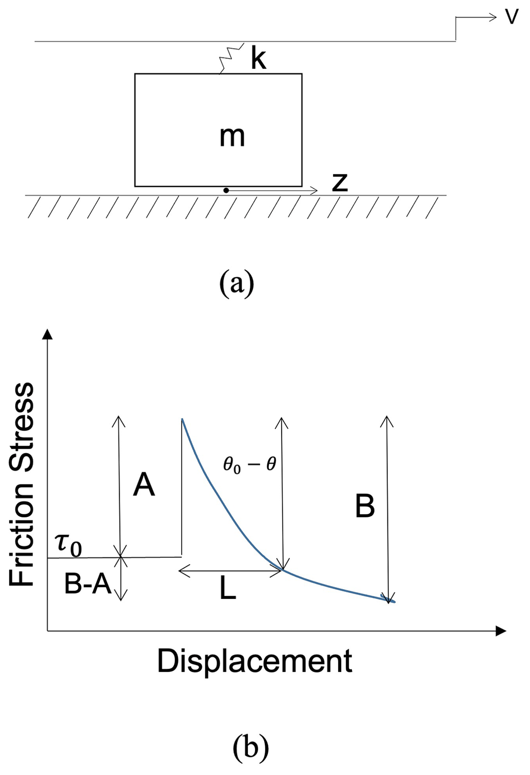
Figure 1 (a) The zero-dimensional (0D) spring–block representation used in this study. k is the spring constant, v is the slip velocity and z (=u) is the slip. (b) A schematic diagram taken from Erickson et al. (2008) illustrating the stress response to a step change in the imposed velocity v of a single spring–block slider model.

We describe the frictional force using a laboratory-derived rate- and state-dependent friction formulation (e.g., Dieterich, 1979; Ruina, 1983; Marone, 1998). This empirical formulation has been used successfully over the last decades to describe the dynamics of sequences of earthquakes, including their spontaneous nucleation, propagation, arrest and post-seismic slip in response to tectonic loading (e.g., Lapusta et al., 2000; Lapusta and Barbot, 2012). As in Rice and Tse (1986), the equation of motion (Eq. 10) for rate- and state-dependent friction equations assuming a slip law for the evolution of state variable θ (Ruina, 1983) can be written as (Erickson et al., 2011, Eq. 6)

$$\begin{array}{}\text{(11)}& {\displaystyle }{F}_i(\dot{z_i},\mathrm{\Theta })={\mathit{\sigma }}_{\mathrm{n}}\left(f^{\ast }+{\mathrm{\Theta }}_i+a\ln {\displaystyle \frac{\dot{z_i}}{v_{\mathrm{0}}}}\right),\text{(12)}& {\displaystyle }\dot{{\mathrm{\Theta }}_i}=-\left({\displaystyle \frac{\dot{z_i}}{L}}\right)\left({\mathrm{\Theta }}_i+b\ln {\displaystyle \frac{\dot{z_i}}{v_{\mathrm{0}}}}\right).\end{array}$$

Here, the capital notation Θ refers to $b\cdot \ln \frac{v_{\mathrm{0}}\mathit{\theta }}{L}$, which is an equivalent yet more convenient description for the rate-and-state friction state variable θ, which can be interpreted as the change in interface strength from reference friction f^∗ (Nakatani, 2001). Furthermore, σ_n is normal stress; v₀ is the reference velocity, which is assumed to be equal to the plate velocity V below; and a, b and L are the associated rate-and-state friction parameters. After a sudden change in the slip rate, parameter a states the direct change in friction. Parameter b describes the evolution towards a new steady-state friction coefficient, where characteristic slip distance L describes the distance taken by state variable θ to reach a new steady-state θ.

In this study, we consider a zero-dimensional (0D) version analyzing a single spring–block slider (Fig. 1a). This model does not take the spatiotemporal correlation between different blocks or fault segments into account. Equation (10) can be rewritten for a single block for nondimensional slip of the block with respect to an initial position on the driving plate u (z in Fig. 1) and nondimensional slip rate v, and it can be solved by assuming v_p=v₀. This can be simplified into three partial differential equations written in terms of dimensionless variables (using $\mathit{\theta }=A\widehat{\mathit{\theta }}$, $v=v_{\mathrm{0}}\widehat{v}$, $u=L\widehat{u}$ and $t=\frac{L}{v_{\mathrm{0}}}\widehat{t}$, where $\widehat{}$ indicates the dimensional variables) as updated from Eq. 2 of Erickson et al. (2008).

$$\begin{array}{}\text{(13)}& {\displaystyle }\dot{\mathrm{\Theta }}=-v(\mathrm{\Theta }+(\mathrm{1}+\mathit{ϵ}\left)\ln v\right),\text{(14)}& {\displaystyle }\dot{u}=v-\mathrm{1},\text{(15)}& {\displaystyle }\dot{v}=-{\mathit{\gamma }}^{\mathrm{2}}\left[u+{\displaystyle \frac{\mathrm{1}}{\mathit{\xi }}}(\mathrm{\Theta }+\ln v)\right],\end{array}$$

where $\mathit{\gamma }=\sqrt{\frac{k}{M}}\frac{L}{v_{\mathrm{0}}}$ is the nondimensional frequency and $\mathit{\xi }=\frac{kL}{A}$ is the nondimensional spring constant (see also Gu et al., 1984). Shear stress τ is derived by multiplying slip by −ξ (e.g., Rice and Tse, 1986).

Finally, the internal parameter $\mathit{ϵ}=\frac{{\mathit{\sigma }}_{\mathrm{n}}^{\prime }(b-a)}{{\mathit{\sigma }}_{\mathrm{n}}^{\prime }a}$ is a key parameter that measures the sensitivity of the velocity relaxation and includes $A=a{\mathit{\sigma }}_{\mathrm{n}}^{\prime }$ and $B=b{\mathit{\sigma }}_{\mathrm{n}}^{\prime }$, where ${\mathit{\sigma }}_{\mathrm{n}}^{\prime }$ is the effective normal stress, as demonstrated in Erickson et al. (2008).

When compared to a slip-weakening friction formulation, the parameter b−a takes the role of a stress drop, whereas a corresponds to the strength excess (Fig. 1b).

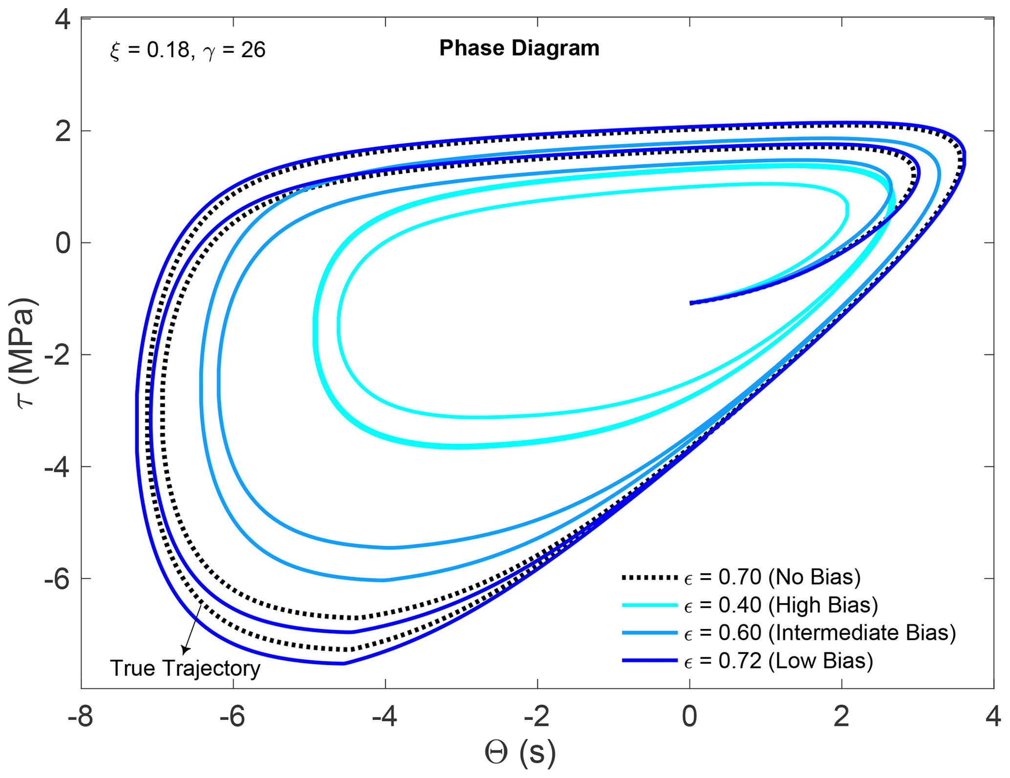
Figure 2 Phase diagram for a Burridge–Knopoff (BK) model with a rate-and-state friction formulation when (1) ϵ = 0.72 (a small-bias case), (2) ϵ = 0.60 (an intermediate-bias case), (3) ϵ = 0.40 (a large-bias case) and (4) the model parameter is equal to the true parameter (a case of no bias).

Table 1 Parameters of the reference model.

2.2.2 Friction parameter ϵ

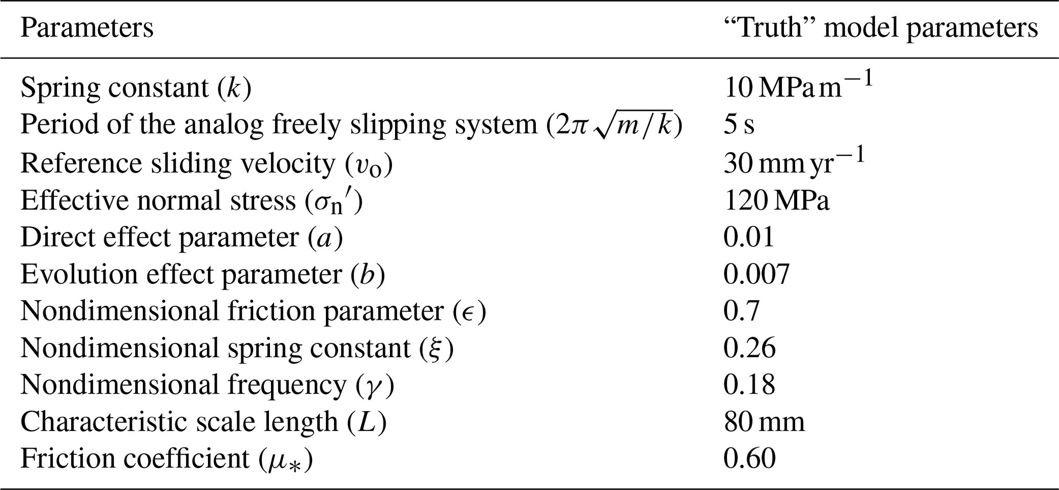
To study stick–slip behavior, we limit our 0D model to a velocity-weakening regime for which $a-b<\mathrm{0}$ and the system generates a stable limit-cycle solution with periodic oscillations (Fig. 2). In nature, earthquakes are far from periodic; however, as we have simplified our model to a 0D system and do not consider the spatiotemporal correlations of the faults, the system generates periodic cycles. The characteristics of the earthquake cycle are strongly influenced by friction parameters a and b. In this study, we address these together and introduce a bias in the prior friction parameter $\mathit{ϵ}=\frac{b-a}{a}$. The parameter values in this work are based on laboratory experiments by Niemeijer and Vissers (2014) on phyllosilicate-rich fault rocks, from which we select the results representative of depths of 6 km. At this depth, five repeat experiments provide a range of ±1 standard deviation (SD) for b−a from 0.00161 to 0.0077 (Fig. 7a in Niemeijer and Vissers, 2014), i.e., equivalent to an ϵ value of 0.161–0.77 for a=0.01. In our synthetic perfect model tests, we define ϵ = 0.7 as the true sensitivity of velocity relaxation. Inspired by the measured b−a SD values, we selected three cases of parameter bias, i.e., ϵ = 0.72 for a small bias of +3 %, ϵ = 0.60 for intermediate bias of −14 % and ϵ = 0.40 for a large bias of −43 %. Figure 2 presents the state trajectories for these three cases. The large impact of the value of ϵ on the system dynamics is evident from the large difference between the trajectory of the simulation with the large parameter bias and that of the true trajectory. All parameters used in the simulations of the “truth” for the fault slip model are summarized in Table 1.

3 Numerical experiments

3.1 State and state-parameter estimation for the seismic-cycle model

In state estimation in the seismic-cycle model, the state x to be estimated is given by $\mathit{x}=[\mathrm{\Theta },\mathit{\tau },v{]}^{\mathrm{T}}$. In the state and parameter estimation, we augment this state vector with

$$\mathit{\xi }=\left[\mathit{ϵ}\right],$$

where ϵ is the poorly known friction parameter. The state vector is then given by $\mathit{z}=[\mathit{x},\mathit{\xi }{]}^{\mathrm{T}}$.

By updating this state vector, we update both the state and the parameter at each new analysis time.

3.2 Experimental design

In the following, we consider a “truth run” with ϵ_t and three different priors with ϵ_m: one with a small bias, one with a medium bias and one with a large bias. To test if data assimilation is indeed capable of estimating the state trajectories, we assimilate synthetic observations of both shear stress and slip rate every four time steps. The reason that we assimilate so frequently is to obtain sufficient information regarding the behavior of the fault in the short coseismic phase (i.e., the phase of the earthquake itself). The performance of the data assimilation is evaluated by comparing state estimates to the true trajectory.

3.3 Twin experiments

As the true state of the fault system is unknown, we validate our data-assimilation algorithms using twin experiments. Using these synthetic experiments, we can assess whether data-assimilation methods are able to correctly evaluate the posterior distribution of the state. For the synthetic truth, we select a forward model run that follows Eqs. (13)–(15). The initial conditions of the three state variables are Θ₀ = 0, d₀ = 6 and v₀ = 1.

For state and parameter estimation, a different approach has been adopted to generate the prior. As we observe that the state variables are highly sensitive to the parameter value, we make sure that prior state variables are fully consistent with the prior parameter values. For this, we use the following procedure:

1. We sample N prior parameters ϵ (where N is the number of particles) from a lognormal distribution with 0.01 SD and a mean of ϵ_m.

2. For each $i=\mathrm{1},\mathrm{\dots },N$ set of parameter values, we run the model forward for a small time duration (around 100 time units) using ${\mathit{ϵ}}_{\mathrm{m}}^{\prime ,i}$.

3. We sample the initial conditions of the state variables (Θ, d, v) from these N forward runs at any random time from each trajectory i.

In this way, each state variable and the parameter chosen in the ensemble (Θ_i, τ_i, v_i, ϵ_i) represent a different trajectory for a different value of ϵ_m. As each particle has a different parameter value, the prior ensemble contains different recurrence times for earthquake slip events.

Synthetic observations are produced by sampling from the synthetic truth and adding an observational error from a Gaussian distribution with an SD of σ_β.

Data-assimilation settings

The experiments are performed with 1000 particles using a sequential-importance resampling (SIR) particle filter. The observations are provided for the two state variables τ and v, as these are most likely to be observable, following the approach and large uncertainties determined by Van Dinther et al. (2019). We sample observations at intervals of four time units (i.e., Δt = 4) and add synthetic observational noise sampled from a normal distribution with zero mean and variance ${{\mathit{\sigma }}_{\mathit{\beta }}}^{\mathrm{2}}\sim N(\mathrm{0},{{\mathit{\sigma }}_{\mathit{\beta }}}^{\mathrm{2}})$. Large assimilation steps can adversely affect data assimilation, as they can miss variations in earthquakes. Thus, it is necessary to choose a short time step. In the present study, observations were sampled at four time units, and the SD of the observation error σ_β was 0.6 for fault shear stress and 1.15 for slip velocity observations. These values are consistent with the estimates of Van Dinther et al. (2019) and Mowafy and Bilbas (2016). The stochastic model error η_t (Eq. 1) for the state evolution is sampled from a normal distribution $\sim N(\mathrm{0},{{\mathit{\sigma }}_{\mathit{\eta }}}^{\mathrm{2}})$ with σ_η = 0.01. We add a value of 0.01 amplitude to represent model error in the fault shear stress τ and state variable Θ and a value of 0.5 for slip velocity v.

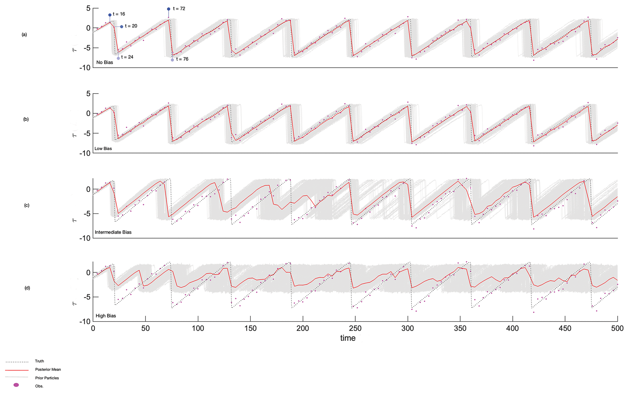
Figure 3 The evolution of 1000 particles along with the posterior mean, observation and truth of state variable τ for state estimation for (a) the case when the model parameter is equal to the true parameter (i.e., a case of no bias; ϵ_m = 0.70), (b) a small-bias case (ϵ_m = 0.72), (c) an intermediate-bias case (ϵ_m = 0.60) and (d) a large-bias case (ϵ_m = 0.40), when ϵ_t = 0.70, γ = 0.26 and ξ = 0.18.

4 Results and analysis

4.1 Case A: state estimation

Figure 3b–d illustrate the evolution of the posterior mean τ (red) and all prior particles (gray) in the three cases of parameter bias and compare it with the reference (no bias) case (Fig. 3a). We refer to the posterior mean as the analysis. When the parameter bias is small, the prior estimates of the fault stress and slip rate evolution capture the truth well, as seen from Fig. 3b. On the other hand, for the intermediate-bias (Fig. 3c) and large-bias (Fig. 3d) cases, the prior state estimation fails to capture the evolution of the shear stress after a few seismic cycles, which complicates the data assimilation going forward. Figure 2b clearly demonstrates that the data assimilation in the large-bias case (ϵ_m = 0.40) is unable to account for the difference in state evolution caused by the parameter bias.

Figure 4 Shear-stress evolution. The coseismic and interseismic phases in the seismic cycle have been highlighted. The time points discussed in the study are $t=\mathrm{16},\mathrm{20},\mathrm{24},\mathrm{72}$ and 76 in the interseismic phase and t=20 in the coseismic phase.

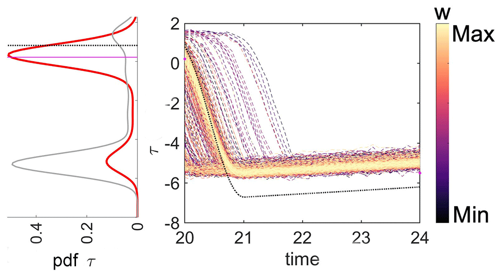
Figure 5 Shear-stress evolution with weight distribution at time t=20. The color of the lines represents the value of the weight, which is a function of the distance between the prior shear-stress estimate and the observation. The red line represents the posterior pdf, the gray line represents the prior pdf, the magenta line shows where the observation stands and the black line is the true state.

Figure 6 Particles in the Θ–τ space for the case of state estimation with (a–e) intermediate bias (ϵ_m = 0.6) and (f–j) no bias (ϵ_m = ϵ_t = 0.7). The points represent the particles in the distribution and the lines represent the trajectories in the phase diagram for the respective values of the parameter ϵ_m. The blue line represents the phase diagram for ϵ_m = 0.6, whereas the black line is for the case in which ϵ_t = 0.7. The sizes and colors of the symbols representing the particles reflect the weight of each particle.

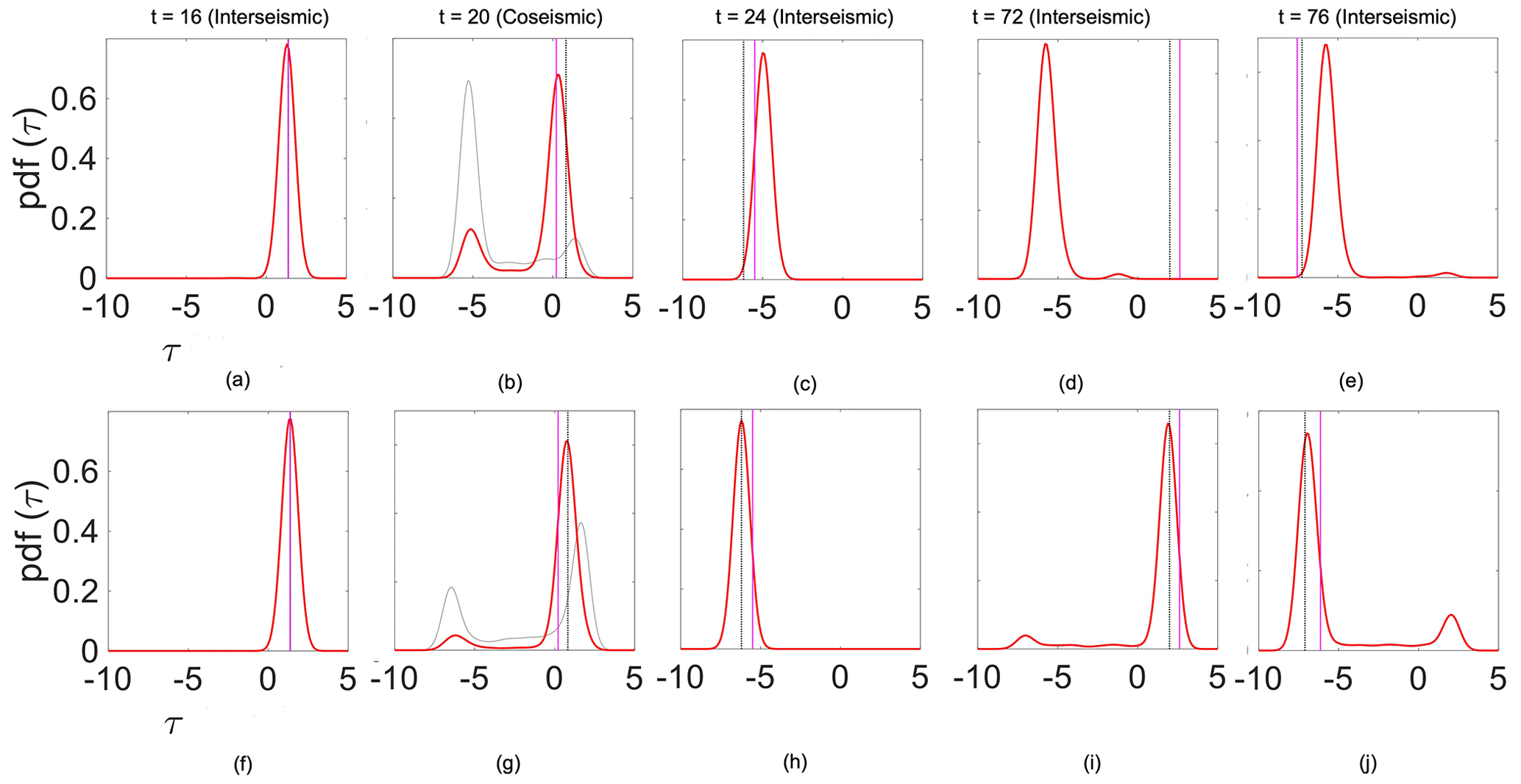
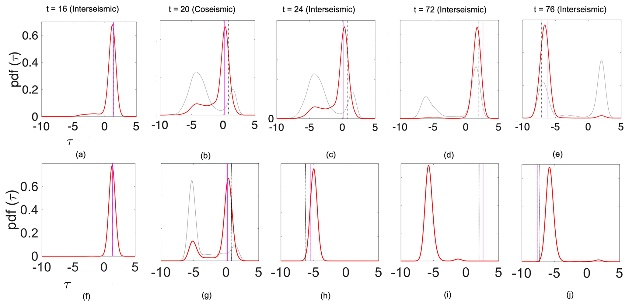
Figure 7 The pdfs representing the posterior mean (red), the prior (gray line), the observation (magenta) and the truth (black line) for the case illustrated in Fig. 6.

To better understand and improve these data-assimilation results, we analyze the results for the experiment with intermediate bias in more detail (Fig. 4). Via the assimilation of data representative of both the interseismic and coseismic periods, we determine whether stress can be estimated. Throughout the paper, we illustrate the stress for a number of assimilation times that represent the time epochs before and after an earthquake (Fig. 3a): $t=\mathrm{16},\mathrm{20},\mathrm{24},\mathrm{72}$ and 76. In the enlarged version of the figure (Fig. 5), we can see the probabilistic estimate of fault shear stress based on the assimilation of coseismic data at t=20. The prior and posterior density represent the particles before and after undergoing resampling, respectively. The mean value of the posterior density of stress corresponds better to the true value than that of the prior density. In fact, at time t=20, the particles closest to the observation (representing a pre-slip condition) have the highest likelihood and, consequently, obtain the highest weights. As a consequence, the posterior density has its peak close to the truth. It should be noted that particles with shear-stress values that are further away from the observations may still obtain high weights because of their fit to the observed slip rate. As a result, the posterior trajectory is close to the observations but fails to completely follow the true trajectory. Figure 6a–j illustrate this further with phase diagrams that show, by means of scatterplots, the distribution of particles in the Θ–τ space. The blue and black lines in the phase diagram in Fig. 2b represent the trajectory of the particles when the model parameter ϵ_m is 0.60 (intermediate bias) and 0.70 (no bias), respectively. The sizes and colors of the symbols indicate the particle weights. Figure 7a–j present the resulting pdf distributions of the corresponding plots in Fig. 6.

The particles with a parameter bias show a phase difference compared with the truth (Fig. 6a–e). Trajectories of particles with lower values of ϵ have a shorter cycle and their Θ–τ trajectories are always ahead of the true trajectories. At time t=16 (i.e., in the interseismic phase), the particles and the truth are almost in sync. However, in the coseismic phase (t=20), minor differences in the state for that specific moment can result in large differences in the state trajectory. In this phase, particles that were previously close to each other are pulled apart. After the coseismic phase (i.e., for t=24), the particles of the biased prior parameter, which have shorter cycles than the truth, reach the interseismic phase of the subsequent earthquake event faster than the truth. The pattern then repeats itself. When there is no bias (Fig. 6f–j), the particles are always in sync with the truth. Compensating for a bias in the prior parameter could also be achieved by changing the assimilation settings. In this study, we explore the effect of (i) increasing the model error and/or (ii) resampling twice rather than once. Using different assimilation settings, it is possible to inflate the ensemble.

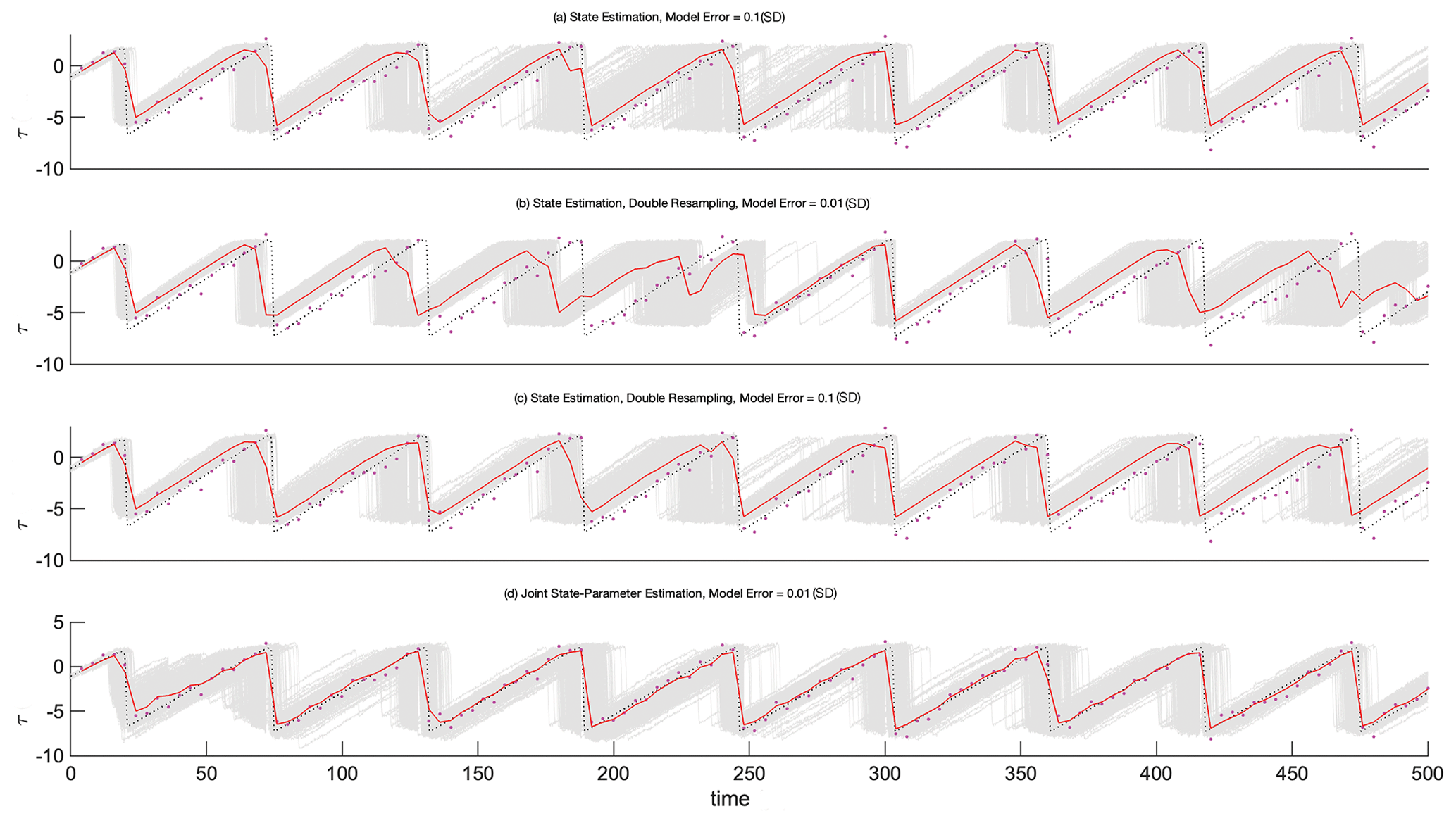
Figure 8 The evolution of particles with time for intermediate bias in state estimation with (a) higher model error (η_t = 0.1), (b) double resampling (η_t = 0.01), (c) a combination of higher model error (η_t = 0.1) and double resampling, and (d) joint state-parameter estimation (η_t = 0.01).

We note that a biased parameter value makes it physically impossible to have Θ and τ in the same phase and amplitude as in the true seismic cycle for an extended period of time. However, with different assimilation settings, it might be feasible to adjust the state such that we can correctly predict the arrival of the next earthquake. Figure 8a–c show the state-estimation results for three different data-assimilation settings, and Fig. 8d presents the case of joint state-parameter estimation. It can be seen from the figure that increasing model error along with frequent resampling leads to more effective compensation for the biased prior parameter than state estimation without these settings (Fig. 3c).

4.2 Case B: increased model error

The model error in the forward model equation represents the imperfections in the model and, thus, maintains ensemble spread. Adding η_t to the forward model equations improves the efficacy of the filter. Choosing a smaller model error reduces the spread, which restricts the solution space considerably.

We find that inclusion of model error has a noticeable positive effect on the posterior estimate (brings the mean of the posterior closer to the truth) when the parameter bias is either small or intermediate.

We observe that increasing the model error causes the prior τ distribution of the particles to have two peaks in the coseismic phase. This was a single peak when the model error was smaller. This shows that increasing model error allows for a larger variety of states in the prior. The phase diagrams for the intermediate bias case when we increase the model error (η_t in Eq. 1) are presented in Fig. S1 in the Supplement.

4.3 Case C: double resampling

Resampling improves the effectiveness of the particle filter by introducing more particles with a state close to the observed state (Sect. 2.1.1). We observe that double resampling retains particles that are in the same interseismic phase as that of the truth (as at t=24). From this, we conclude that double resampling can be useful with respect to retaining more particles “in sync” with the truth in the distribution, but additional spread in the ensemble is required to shift the posterior distribution more towards the truth. It is also important to highlight that we observe a double peak at 250 time steps in Fig. 8b, which represents the double-resampling experiment. At this (250th) time step, the data-assimilation analysis does not fit the observations well. A similar mismatch is observed after approximately 500 time steps in this experiment. At these moments, double resampling effectively increases the spread in the particles to such an extent that the constraint to the shear-stress observations becomes less strong. Hence, we can conclude that, although it can be useful with respect to retaining important particles in the prior distribution, double resampling is not as effective with respect to increasing the ensemble spread compared with increased model error (Fig. 8a). The effect of double resampling on the posterior distribution for an intermediate bias is provided in Fig. S2 in the Supplement.

4.4 Case D: increased model error and double resampling

We study the effect of increasing the model error with consequent double resampling on the posterior estimates and use the term “combined adjustment” for this data-assimilation setting. The posterior distribution of stress for the combined adjustment captures the truth distinctly better compared with the case with model error only. There is no significant difference in the forecasting ability of the prior particle distribution in the first seismic cycle for the combined adjustment. Increasing model error and double resampling both increase the variability within the particles. However, at time t=76, after the coseismic phase, particles of this combined adjustment experiment are no longer fully in sync with the truth. The effect of combined adjustment on the posterior distribution for an intermediate bias is provided in Fig. S3 in the Supplement.

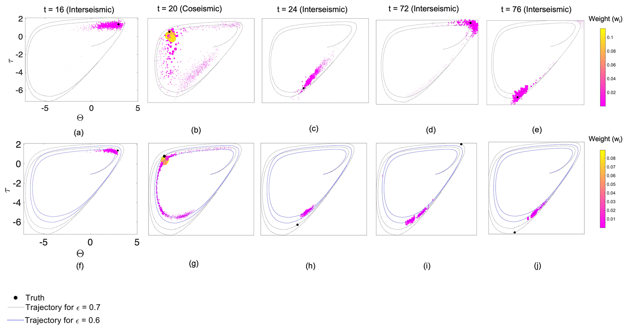
Figure 9 The Θ–τ phase diagrams for the case with (a–e) state-parameter estimation and (f–j) state estimation for intermediate bias. The use of colors and lines is the same as in Fig. 6.

Figure 10 The pdfs for the case with (a–e) joint state-parameter estimation and (f–j) state estimation with intermediate bias in Fig. 9.

4.5 Case E: joint state-parameter estimation

Figure 9 presents the results for state-parameter estimation as phase diagrams. Figure 10 presents the corresponding pdf distributions of these phase diagrams. Not surprisingly, joint state-parameter estimation (Fig. 9a–e) improves the posterior distribution compared with the case of state estimation (Fig. 9f–j).

The parameter estimate gradually comes close to its true value after a certain time period. In the state-parameter estimation case, the parameter estimate gradually changes from its prior (biased) value towards the correct estimate of ϵ = 0.7 and then remains at that value. Hence, in this case, the state variables are improved in the next seismic cycle, which is not the case in state estimation. From this, we can conclude that joint state-parameter estimation is the most effective approach for seismic-cycle estimation in the presence of a parameter bias in this case. It is important to note that the state-parameter estimate leads not only to a reasonably good posterior estimate of the state at these selected time steps but also at all assimilation time steps in the period considered, i.e., from t=4 to t=500 (Fig. 4).

To evaluate the overall accuracy of the state and the joint state-parameter estimation for the different biased-parameter cases, we perform a regression analysis. The results in Fig. 11 show how close the posterior estimates of the different experiments are to the truth using the R-squared (R²) value. We find that state estimation is efficient when the parameter bias is small, with an R² value of 0.99. For the intermediate-bias case, the setting of increasing the model error to 0.1 and consequent resampling with a smaller model error of 0.01 SD (standard deviation) results in an R² value of 0.61. However, for all of the cases, the joint state-parameter estimation leads to significantly higher R² values and, hence, improved state estimates compared with the cases with state estimation only. This confirms our conclusion from Sect. 4.5.

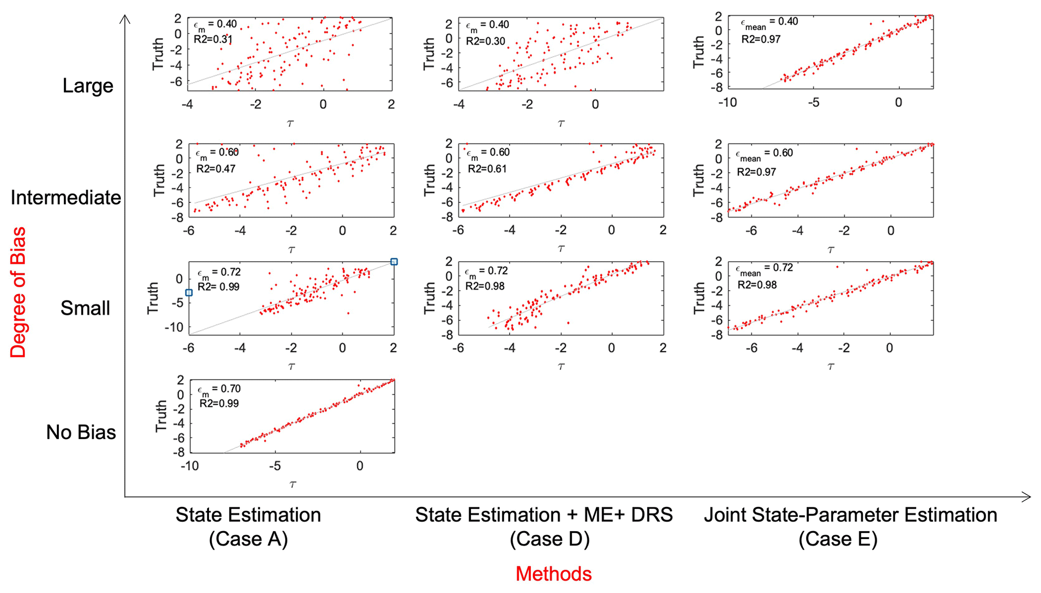
Figure 11 Comparison of regression between the estimate of τ and the true τ, showing the corresponding R² values for the three bias cases (rows) and for different assimilation approaches (columns). The red dots indicate the estimated values or the posterior and true τ values at the observation times. A diagonal line is added for reference.

5 Discussion

The results of this study illustrate the implications of parameter bias in data-assimilation applications for seismic-cycle modeling. They show that it is feasible to apply a particle filter to a fault slip model; moreover, they reveal that uncertainties in friction parameters can be accounted for by either directly estimating these parameters or via a larger model error. By accounting for these improved parameter estimates, fault state estimates can also be improved. This demonstrates that a possible trade-off between estimating shear stress and friction can be effectively accounted for using data-assimilation methods. In other words, data assimilation is able to separate error contributions due to uncertainties in friction (i.e., shear over normal stress) from uncertainties in estimates of a fault's shear stresses. This suggests that potentially large uncertainties in friction do not hamper the further development of data-assimilation methods nor physics-based seismic hazard assessment.

The simplest and most effective approach to deal with parameter bias depends on the degree of parameter bias observed. For laboratory experiments with increased accuracy, one can potentially still use and tune state estimation (e.g., via increasing model error). However, for observed uncertainties in laboratory experiments such as in Niemeijer and Vissers (2014), particularly when also accounting for uncertainties under in situ conditions (e.g., effective pressure and thermal conditions and the amount of displacement) and in laboratory setups (e.g., sample type with or without gouge), state-parameter estimation is clearly the best and the required approach. It is remarkable to observe that any degree of bias can be dealt with equally effectively by accounting for state-parameter estimation (Fig. 11). This suggests that, even upon extrapolation to significantly larger biases, state-parameter estimation can be an effective solution for earthquake-cycle problems.

It is important to remember that these findings are based on the performance of state update and state-parameter update algorithms for a simplified nonlinear physics-based model in synthetic experiments. Some limitations that are still present in this pioneering study, which eventually need to be addressed, include the following:

• In this study, we assimilate both the fault shear-stress and the slip rate observations on the plate interface. However, we have also conducted experiments only assimilating the fault shear-stress observations. In the latter case, it is observed that the state estimate yields better fits to the truth compared with the case in which we assimilate both types of observations or only the slip rate. Assimilating slip rate observations leads to lower weight values owing to their relatively high observation error. This affects the posterior estimate. However, a thorough study still needs to be conducted to identify which observations provide the most meaningful information when assimilated in earthquake-cycle models.

• In this study, we focus only on the uncertainty with respect to parameter ϵ. It can be seen from Eqs. (13)–(15) that the highly uncertain characteristic slip length L also impacts fault states and cycle characteristics.

• Typically, earthquake forecasting is approached in a probabilistic manner (e.g., Marzocchi et al., 2017). Kinematic inversions of earthquake global positioning system (GPS) data have been used to estimate frictional properties in afterslip areas (e.g., Miyazaki et al., 2004; Hsu et al., 2006) but not for the estimation of earthquake dynamics. As outlined by Van Dinther et al. (2019), data assimilation for earthquake sequences has the advantage that it can account for measurement and model errors, non-Gaussian probabilities and sequential updating as data become available. The results of this study demonstrate how, for a highly simplified representation of earthquake cycles, nonlinear data assimilation provides a means to account for both measurement errors and parameter biases. It also highlights how observations can be included as they become available. While particle filters are not computationally efficient, they can propagate the full error distribution, which makes them attractive for the estimation and forecasting of highly nonlinear processes like earthquake generation.

• Another point of attention is the selection of the number of particles required for a correct sampling of the prior. On the one hand, increasing the number of particles can improve estimation accuracy, but limited computational resources can make this impractical. On the other hand, having a lower number of particles increases the risk of filter degeneracy. In this study, we initially used 50 and 100 particles but increased the number of particles to 1000 to avoid degeneracy. Realization of 1000 particles may be computationally expensive for models that are more complex than the model used here. Improved sampling techniques, such as using a proposal density function, or using a particle flow (e.g., Hu and Van Leeuwen, 2021) could help one to reduce computational costs while maintaining the advantage of a nonlinear filtering method.

• An additional point worth mentioning is the use of synthetic observations for fault displacement and velocities for data assimilation in this study. In realistic applications, the assumptions that we have made with respect to data-assimilation frequency and the SD and distribution of the observational errors may not be valid. However, if we know the distribution of the measurement errors, we can use that information to choose the relevant likelihood function, which can greatly effect our fault estimates. Fault shear-stress observations are usually not available or are subject to large errors if they are available. In contrast, fault velocities can be observed fairly accurately using GPS; this has been discussed by Van Dinther et al. (2019), who demonstrated that stress measurements are useful despite their large errors. Following Van Dinther et al. (2019), we emphasize the need to conduct additional sensitivity studies in order to understand the implications of factors such as data gaps, outliers and instrumental noise before our proposed methods can be used on real data.

• It is also very important to highlight the reason behind selecting a 0D model for this study. Simplified fault slip models are computationally efficient tools that help us to understand the physics behind earthquake dynamics. A study by Li et al. (2022) compared the simulation of earthquakes in 0D, 1D, 2D and 3D models and found that lower-dimension models (0D and 1D) qualitatively represent the same dynamics as 2D and 3D models. Although 0D models cannot simulate the full complexity of earthquake physics, they have the advantage that they are computationally inexpensive and provide the user with a tractable conceptual description of earthquake physics and the importance of the friction parameter. In our case, we were interested in investigating the effect of frictional parameter bias on the estimated fault states in earthquake-cycle models. Hence, in the present work, we investigated a simplified version of a Burridge–Knopoff spring–block slide model in a simplified 0D form. Eventually, in order to accurately simulate the behavior of real earthquake faults, 1D, 2D and 3D simulation models will be required (e.g., Li et al., 2022).

Nonetheless, simplified models provide useful insights to solve more complex problems. This is an important stepping stone in the development of data-assimilation applications for the simulation of more realistic earthquake cycles. Future developments for these purposes, addressing the above limitations, could utilize other methods explicitly accounting for parameter bias in the data-assimilation scheme in order to obtain a better accuracy (e.g., Dee and Da Silva, 1998; Sørensen and Madsen, 2004; Chepurin et al., 2005; Auligné et al., 2007; Li et al., 2009; Du et al., 2020).

6 Conclusions

In this study, we demonstrated the effect of a parameter bias in an earthquake-cycle model on the estimated states with data assimilation. Synthetic, noisy observations of the shear stress and slip velocity on the fault plate interface were assimilated with state and state-parameter estimation methods using a particle filter. In our forward model, the shear-stress estimates strongly depend on the friction parameter ϵ. Therefore, an inaccurate representation of this parameter would impact the stress estimates and forecast cycles obtained using this model. To quantify this impact, we considered three different magnitudes of biases with respect to the true parameter ϵ_t = 0.7: (i) small bias (model parameter ϵ_m = 0.72), (ii) intermediate bias (model parameter ϵ_m = 0.60) and (iii) large bias (model parameter ϵ_m = 0.40).

For a small bias in friction parameter ϵ, we find that state estimation is most effective (R² = 0.99 for the regression between the estimated and true shear stress). In the case of an intermediate bias, state estimation alone is less effective (R² = 0.47). However, by increasing the prior model error and adding a second resampling step in the data-assimilation approach, the results can be improved (R² = 0.61). Nonetheless, state-parameter estimation in this case is best (R² = 0.97). In the case of a large parameter bias, state-parameter estimation (R² = 0.97) is a significantly more effective manner to reconstruct the true state than state estimation (R² = 0.31) or improved state estimation with combined adjustments (R² = 0.30). This suggests that state-parameter estimation using data assimilation could be an effective method to improve forecasts of frequently recurring fault slip events.