the Creative Commons Attribution 4.0 License.
the Creative Commons Attribution 4.0 License.
 | 25 Feb 2022
Fractional relaxation noises, motions and the fractional energy balance equation
We consider the statistical properties of solutions of the stochastic fractional relaxation equation and its fractionally integrated extensions that are models for the Earth's energy balance. In these equations, the highest-order derivative term is fractional, and it models the energy storage processes that are scaling over a wide range. When driven stochastically, the system is a fractional Langevin equation (FLE) that has been considered in the context of random walks where it yields highly nonstationary behaviour. An important difference with the usual applications is that we instead consider the stationary solutions of the Weyl fractional relaxation equations whose domain is −∞ to t rather than 0 to t.
An additional key difference is that, unlike the (usual) FLEs – where the highest-order term is of integer order and the fractional term represents a scaling damping – in the fractional relaxation equation, the fractional term is of the highest order. When its order is less than (this is the main empirically relevant range), the solutions are noises (generalized functions) whose high-frequency limits are fractional Gaussian noises (fGn). In order to yield physical processes, they must be smoothed, and this is conveniently done by considering their integrals. Whereas the basic processes are (stationary) fractional relaxation noises (fRn), their integrals are (nonstationary) fractional relaxation motions (fRm) that generalize both fractional Brownian motion (fBm) as well as Ornstein–Uhlenbeck processes.
Since these processes are Gaussian, their properties are determined by their second-order statistics; using Fourier and Laplace techniques, we analytically develop corresponding power series expansions for fRn and fRm and their fractionally integrated extensions needed to model energy storage processes. We show extensive analytic and numerical results on the autocorrelation functions, Haar fluctuations and spectra. We display sample realizations.
Finally, we discuss the predictability of these processes which – due to long memories – is a past value problem, not an initial value problem (that is used for example in highly skillful monthly and seasonal temperature forecasts). We develop an analytic formula for the fRn forecast skills and compare it to fGn skill. The large-scale white noise and fGn limits are attained in a slow power law manner so that when the temporal resolution of the series is small compared to the relaxation time (of the order of a few years on the Earth), fRn and its extensions can mimic a long memory process with a range of exponents wider than possible with fGn or fBm. We discuss the implications for monthly, seasonal, and annual forecasts of the Earth's temperature as well as for projecting the temperature to 2050 and 2100.
- Article
(8902 KB) - Full-text XML
- BibTeX
- EndNote


Over the last decades, stochastic approaches have rapidly developed and have spread throughout the geosciences. From early beginnings in hydrology and turbulence, stochasticity has made inroads in many traditionally deterministic areas. This is notably illustrated by stochastic parameterizations of numerical weather prediction models, e.g. Buizza et al. (1999), and the “random” extensions of dynamical systems theory, e.g. Chekroun et al. (2010).
In parallel, pure stochastic approaches have developed primarily along two distinct lines. One is the classical (integer-ordered) stochastic differential equation approach based on the Itô or Stratonovich calculus that goes back to the 1950s (see the useful review by Dijkstra, 2013). The other is the scaling strand that encompasses both linear (monofractal, Mandelbrot, 1982) and nonlinear (multifractal) models (see the review by Lovejoy and Schertzer, 2013) that are based on phenomenological scaling models, notably cascade processes. These and other stochastic approaches have played important roles in nonlinear geoscience.
Up until now, the scaling and differential equation strands of stochasticity have had surprisingly little overlap. This is at least partly for technical reasons: integer-ordered stochastic differential equations have exponential Green functions that are incompatible with wide-range scaling. However, this shortcoming can – at least in principle – be easily overcome by introducing at least some derivatives of fractional order. Once the (typically) ad hoc restriction on integer orders is dropped, the Green functions are based on “generalized exponentials” that in turn are based on fractional powers (see the review by Podlubny, 1999). The integer-ordered stochastic equations that have received the most attention are thus the exceptional, non-scaling special cases. In physics they correspond to classical Langevin equations; in geophysics and climate modelling, they correspond to the linear inverse modelling (LIM) approach that goes back to Hasselmann (1976) and later elaborated notably by Penland and Magorian (1993), Penland (1996), Sardeshmukh et al. (2000), Sardeshmukh and Sura (2009) and Newman (2013). Although LIM is not the only stochastic approach to climate, in two recent representative multi-author collections (Palmer and Williams, 2010; Franzke and O'Kane, 2017), all 32 papers shared the integer-ordered assumption (a single exception being Watkins, 2017; see also Watkins et al., 2020).
Under the title “Fractal operators”, West et al. (2003) review and emphasize that, in order to yield scaling behaviours, it suffices that stochastic differential equations contain fractional derivatives. However, when it is the time derivatives of stochastic variables that are fractional – fractional Langevin equations (FLEs) – then the relevant processes are generally non-Markovian (Jumarie, 1993), so that there is no Fokker–Planck (FP) equation describing the corresponding probabilities. Even in the relatively few cases where the FLE has been studied, the fractional terms are generally models of viscous damping, so that the highest-order terms are still integer-ordered (an exception is Watkins et al., 2020, who mention “fractionally integrated FLE” of the type studied here but without investigating its properties). Integer-ordered terms have the convenient consequence of regularizing the solutions, so that they are at least root mean square continuous; in this paper the highest-order derivatives are fractional, so that when the highest-order terms are , the solutions are “noises”, i.e. generalized functions that must be smoothed in order to represent physically meaningful quantities.
An additional obstacle is that – as with the simplest scaling stochastic model, fractional Brownian motion (fBm, Mandelbrot and Van Ness, 1968) – we expect that the solutions will not be semi-martingales and hence that the Itô calculus used for integer-ordered equations will not be applicable (see Biagini et al., 2008). This may explain the relative paucity of mathematical literature on stochastic fractional equations (see however Karczewska and Lizama, 2009). In statistical physics, starting with Mainardi and Pironi (1996), Metzler and Klafter (2000) and Lutz (2001) helped with numerics; the FLE (and a more general “Generalized Langevin Equation”, Kou and Sunney Xie, 2004; Watkins et al., 2019) has received a little more attention as a model for (nonstationary) particle diffusion (see West et al., 2003, for an introduction, or Vojta et al., 2019, for a more recent example). These technical aspects may explain why the statistics of the resulting processes are not available in the literature.
Technical difficulties may also explain the apparent paradox of continuous-time random walks (CTRWs) and other approaches to anomalous diffusion that involve fractional equations. While CTRW probabilities are governed by the deterministic fractional-ordered generalized fractional diffusion equation (e.g. Hilfer, 2000; Coffey et al., 2012), the walks themselves are based on specific particle jump models rather than (stochastic) Langevin equations. Alternatively, a (spatially) fractional-ordered Fokker–Planck equation may be derived from an integer-ordered but nonlinear Langevin equation for a diffusing particle driven by an (infinite-variance) Levy motion (Schertzer et al., 2001).
In nonlinear geoscience, it is all too common for mathematical models and techniques developed primarily for mathematical reasons to be subsequently applied to the real world. This approach – effectively starting with a solution and then looking for a problem – occasionally succeeds, yet historically the converse has generally proved more fruitful. The proposal that an understanding of the Earth's energy balance requires the fractional energy balance equation (FEBE, Lovejoy et al., 2021, announced in Lovejoy, 2019a) is an example of the latter. First, the scaling exponent of macroweather (monthly, seasonal, interannual) temperature stochastic variability was determined () and shown to permit skillful global temperature predictions (Lovejoy, 2015b; Lovejoy et al., 2015; Del Rio Amador and Lovejoy, 2019), and then it was extended to regional temperatures (at resolution) (Del Rio Amador and Lovejoy, 2019, 2021a, b). The latter papers showed how the long-memory high-frequency approximation to the FEBE can not only make state-of-the-art multi-month temperature forecasts, but also how the corresponding simulations generate emergent properties such as realistic El Niño events.
In parallel, the multidecadal deterministic response to external (anthropogenic, deterministic) forcing was shown to also obey a scaling law but with a different exponent (Hébert, 2017; Lovejoy et al., 2017; Procyk et al., 2020, 2022; Procyk, 2021), . It was only then realized that the order h FEBE naturally accounts for both the high- and low-frequency global temperature exponents with and , with both empirical exponents recovered with a FEBE of order . The realization that the FEBE fit these basic empirical facts motivated the present research into its statistical properties, including its predictability.
In the EBE, energy storage is modelled by a uniform slab of material, implying that, when perturbed, the temperature exponentially relaxes to a new thermodynamic equilibrium. However, as reviewed in Lovejoy and Schertzer (2013), both conventional global circulation models and observations show that atmospheric, oceanic and surface (e.g. topographic) structures are spatially scaling. A consequence is that the temperature relaxes to equilibrium in a power law manner. This motivated earlier approaches (van Hateren, 2013; Rypdal, 2012; Hébert, 2017; Lovejoy et al., 2017) to postulate that the climate response function (CRF) itself is scaling. However, these models require either ad hoc truncations or imply infinite sensitivity to small perturbations (Rypdal, 2015; Hébert and Lovejoy, 2015).
The FEBE instead situates the scaling in the energy storage processes; this is the physical basis for the phenomenological derivation of the FEBE proposed in Lovejoy et al. (2021), and the zeroth-order term guarantees that equilibrium is reached after long enough times. The scaling of the basic physical quantities in both time and space motivates the study of the FEBE and its fractionally integrated extensions discussed below with temperature treated as a stochastic variable. The FEBE determines the Earth's global temperature when the energy storage processes are scaling and modelled by a fractional time-derivative term. Recently, analysis of the atmospheric radiation budget has shown that, at least over some regions, the internal component of the radiative forcing may itself be scaling: this justifies the consideration of the extensions to fGn forcing.
The FEBE differs from the classical energy balance equation (EBE) in several ways. Whereas the EBE is integer-ordered and describes the deterministic, exponential relaxation of the Earth's temperature to equilibrium, the FEBE is of fractional order, and because it is both deterministic and stochastic, it unites all the forcings and responses into a single model. Whereas the stochastic part represents the forcing and response to the unresolved degrees of freedom – the “internal variability” – and is treated as a zero mean Gaussian noise, the deterministic part represents the external (e.g. anthropogenic) forcing and the forced response modelled by the total external forcing. Complementary work (Procyk et al., 2020, 2022; Procyk, 2021) uses the deterministic FEBE as the basic model for the response to external forcing, but its Bayesian parameter estimation uses the stochastic FEBE to characterize the likelihood function of the residuals assumed to be the responses to stochastic internal forcing and governed by the same equation. It thus avoids the ad hoc error models involved in conventional Bayesian parameter estimation. The result is a parsimonious, FEBE projection of the Earth's temperature to 2100 that has much lower uncertainty than the classical global circulation model alternative. This is the first time that classical general circulation model climate projections have been confirmed by an independent, qualitatively different, approach.
An important but subtle EBE–FEBE difference is that, whereas the former is an initial value problem whose initial condition is the Earth's temperature at t=0, the FEBE is effectively a past value problem whose prediction skill improves with the amount of available past data, and – depending on the parameters – it can have an enormous memory (Del Rio Amador and Lovejoy, 2021b). To understand this, recall that an important aspect of fractional derivatives is that they are defined as convolutions over various domains. To date, the main one that has been applied to physical problems is the Riemann–Liouville (and the related Caputo) fractional derivative specialized to convolutions over the interval between an initial time=0 and a later time t. With one or two exceptions, this is the domain considered in Podlubny's mathematical monograph on deterministic fractional differential equations (Podlubny, 1999) as well as in the stochastic fractional physics discussed in West et al. (2003), Herrmann (2011), Atanackovic et al. (2014), and most of the papers in Hilfer (2000) (with the partial exceptions of Schiessel et al., 2000, and Nonnenmacher and Metzler, 2000). A key point of the FEBE is that it is instead based over semi-infinite domains – here from −∞ to t – often called Weyl fractional derivatives. This is the natural range to consider for the Earth's energy balance, and it is needed to obtain statistically stationary responses. Random walk problems involving fractional equations over the domain 0 to t can be dealt with using Laplace transform techniques. In comparison, the Earth's temperature balance involves statistically stationary stochastic forcings that are more conveniently dealt with using Fourier techniques.
We have mentioned that the FEBE can be derived phenomenologically where the fractional derivative of order h term represents the energy storage processes (Lovejoy et al., 2021). In this approach order h is an empirically determined parameter with h=1 corresponding to the classical (exponential) exception. Alternatively, it may derived from a more fundamental starting point, the classical heat equation – the same starting point as the classical Budyko–Sellers energy balance models (Budyko, 1969; Sellers, 1969). Recently it was shown with the help of Babenko's operator method that the special FEBE – the half-ordered energy balance equation (HEBE) – could be derived analytically from the classical heat equation (Lovejoy, 2021a, b).
To obtain the HEBE, it is sufficient to follow the Budyko–Sellers approach but to avoid one of their key approximations. The Earth's atmosphere and ocean are driven by local imbalances in radiative fluxes. While Budyko–Sellers models simply redirect this flux away from the Equator, the HEBE improvement (Lovejoy, 2021a, b) is to instead use the mathematically correct radiative–conductive surface boundary conditions. When this is done in the classical energy transport equation, one obtains an important special case of the FEBE, the half-order EBE or HEBE. The use of half-order derivatives in the heat equation is completely classical and goes back to at least Oldham (1973), Oldham and Spanier (1972), Babenko (1986), Magin et al. (2004), and Sierociuk et al. (2013). The extension to can be obtained using the same mathematical techniques by starting with the fractional generalization of the classical heat equation, the fractional heat equation. Further generalizations are also possible and will be reported elsewhere.
The choice of a Gaussian white noise forcing was made not so much for its theoretical simplicity as for its physical realism. Using scaling to divide atmospheric dynamics into dynamical ranges (Lovejoy, 2013, 2015a, 2019b), the main ones are weather, macroweather and climate. While the temperature variability in both space and time is generally highly intermittent (multifractal), there is one exception: the temporal macroweather regime (starting at the lifetime of planetary structures – roughly 10 d – up until the climate regime at much longer scales). Macroweather is the regime over which the FEBE applies, and it has exceptionally low intermittency: temporal (but not spatial) temperature anomalies are not far from Gaussian (Lovejoy, 2018). Responses to multifractal or Levy process FEBE forcings may however be of interest elsewhere.
This paper is structured as follows. In Sect. 2 we present the fractional relaxation equation, forced by a Gaussian white noise as a natural generalization of classical fractional Brownian motion, fractional Gaussian noise and Ornstein–Uhlenbeck processes (Sect. 2.1 and 2.2). When forced by Gaussian white noises, the solutions define the corresponding fractional relaxation motions (fRm) and fractional relaxation noises (fRn). We consider further extensions to the case where the equation is forced by a scaling noise fGn (Sect. 2.3, Eqs. 21 and 22). This is equivalent to considering the fractionally integrated fractional relaxation equation with white noise forcing. In Sect. 2, we first solve the equations in terms of Green's functions and then introduce powerful Fourier techniques that yield integral representations of the second-order statistics, including autocorrelations, structure functions (Eqs. 33 and 35), Haar fluctuations and spectra (with many details in Appendix A and in Appendix B, we derive the properties of the HEBE special case). In Sect. 3, we develop both short- and long-time (asymptotic) series expansions for the statistics (Eqs. 49 and 51), and we display and discuss sample fRn and fRm processes. In Sect. 4 we discuss the problem of prediction – important for macroweather forecasting – and derive expressions for the optimum predictor (Eq. 63) and its theoretical prediction skill as a function of forecast lead time (Eq. 68). In Sect. 5 we conclude.
We could note that the paper is somewhat complex due to the necessity of developing several approaches: Fourier for the main integral representations (Sect. 2), Laplace for the asymptotic expansions (Sect. 3), and real space for the predictability results (Sect. 4).
2.1 fRn, fRm, fGn and fBm
In the introduction, we outlined physical arguments that the Earth's global energy balance could be well modelled by the fractional energy balance equation. Taking T as the globally averaged temperature, τ as the characteristic timescale for energy storage/relaxation processes, F as the (stochastic) forcing (energy flux; power per area), and s as the climate sensitivity (temperature increase per unit flux of forcing), the FEBE can be written in Langevin form as
where the Riemann–Liouville fractional derivative symbol is defined as
where Γ is the standard gamma function. Derivatives of order ν>1 can be obtained using , where m is the integer part of ν, and then applying this formula to the mth ordinary derivative. The main case studied in applications (e.g. random walks) is a=0, so that Laplace transform techniques are often used (alternatively, the somewhat different Caputo fractional derivative is used). However, here we will be interested in : the Weyl fractional derivative , which is naturally handled by Fourier techniques (Sect. 2.4 and Appendices A and B), and, in this case, this distinction is unimportant.
Since Eq. (1) is linear, by taking ensemble averages, it can be decomposed into deterministic and random components with the former driven by the mean forcing external to system 〈F〉 and the latter by the fluctuating stochastic component F−〈F〉 representing the internal forcing driving the internal variability. The deterministic part has been used to project the Earth's temperature throughout the 21st century (Procyk et al., 2020, 2022); in the following we consider the simplest purely stochastic model in which 〈F〉=0 and F=γ, where γ is a Gaussian “delta-correlated” and with unit amplitude white noise:
In Hébert (2017), Lovejoy et al. (2017), and Hébert et al. (2021), it was argued on the basis of an empirical study of ocean–atmosphere coupling that τr≈2 years, while recent work indicates a value somewhat higher, ≈5 years (Procyk et al., 2022). At high frequencies, Lovejoy et al. (2015) and Del Rio Amador and Lovejoy (2019, 2021a) showed that the value h≈0.4 reproduced the Earth's temperature at scales <τ as well as for macroweather scales (longer than the weather regime scales of about 10 d) but still <τ. Procyk et al. (2020) also used the FEBE to estimate (the global) (90 % confidence interval), and the amplitude of the radiative forcing at monthly resolution was [0.89;1.42] W m−2 (90 % confidence interval).
When , Eq. (1) with γ(t) replaced by a deterministic forcing is a fractional generalization of the usual (h=1) relaxation equation; when , it is the “fractional oscillation equation”, a generalization of the usual (h=2) oscillation equation (Podlubny, 1999).
To simplify the development, we use the relaxation time τ to nondimensionalize time, i.e. to replace time by to obtain the canonical Weyl fractional relaxation equation:
for the nondimensional process Uh. The dimensional solution of Eq. (1) with nondimensional γ=sF is simply ), so that in the nondimensional Eq. (4), the characteristic transition “relaxation” time between dominance by the high frequency (differential) and the low frequency (Uh term) is t=1. Although we give results for the full range – i.e. both the “relaxation” and “oscillation” ranges – for simplicity, we refer to the solution Uh(t) as “fractional relaxation noise” (fRn) and to Qh(t) as “fractional relaxation motion” (fRm). Note that fRn is only strictly a noise when .
In dealing with fRn and fRm, we must be careful of various small and large t divergences. For example, Eqs. (1) and (4) are the fractional Langevin equations corresponding to generalizations of integer-ordered stochastic diffusion equations: the classical h=1 case is the Ohrenstein–Uhlenbeck process. Since γ(t) is a “generalized function” – a “noise” – it does not converge at a mathematical instant in time, and it is only strictly meaningful under an integral sign. Therefore, a standard form of Eq. (4) is obtained by integrating both sides by order h (i.e. by differentiating by −h and assuming that differentiation and integration of order h commute):
(see e.g. Karczewska and Lizama, 2009). The white noise forcing in the above is statistically stationary; the solution for Uh(t) is also statistically stationary. It is tempting to obtain an equation for the motion Qh(t) by integrating Eq. (4) from −∞ to t to obtain the fractional Langevin equation , where W is the Wiener process (a standard Brownian motion) satisfying dW=γ(t)dt. Unfortunately the Wiener process-integrated −∞ to t almost surely diverges, and hence we relate Qh to Uh by an integral from 0 to t.
In the high-frequency limit, the derivative dominates, and we obtain the simpler fractional Langevin equation
whose solution Fh is the fractional Gaussian noise process (fGn, not to be confused with the forcing) and whose integral Bh is fractional Brownian motion (fBm). We thus anticipate that Fh and Bh are the high-frequency limits of fRn and fRm.
2.2 Green's functions
Although it will turn out that Fourier techniques are very convenient for calculating the statistics, there are also advantages to classical (real-space) approaches, and in any case they are needed for studying the predictability properties (Sect. 4). We therefore start with a discussion of Green's functions that are the classical tools for solving inhomogeneous linear differential equations:
where and are Green's functions for the differential operators corresponding respectively to and . Note that, due to causality, all Green's functions used in this paper vanish for t<0.
and are the usual “impulse” (Dirac) response Green's functions (hence the subscript “0”). For the differential operator Ξ, they satisfy
Integrating this equation, we find an equation for their integrals G1,h, which are thus “step” (Heaviside, subscript “1”) response Green functions satisfying
where Θ is the Heaviside (step) function (=0 for t<0, =1 for t≥0). The inhomogeneous equation
has a solution in terms of either an impulse or a step Green function:
the equivalence being established by integration by parts with the conditions and . The use of the step rather than impulse response is standard in the energy balance equation literature since it gives direct information on energy balance and the approach to equilibrium (see e.g. Lovejoy et al., 2021). The step response for the noise is also the basic impulse response function for the motion.
For fGn, Green's functions are simply the kernels of the fractional integrals
obtained by integrating both sides of Eq. (6) by order h. We conclude that
For fRn, we now recall some classical results useful in geophysical applications. First, these Green functions are often equivalently written in terms of Mittag–Leffler functions (“generalized exponentials”), Eα,β.
To lighten the notation in Eq. 14 and in the following, we suppress the superscripts for fRn and fRm processes. A convenient feature of Mittag–Leffler functions is that they can easily be integrated by any positive order α:
(Podlubny, 1999). As mentioned, the constraint t>0 is due to causality, and physical Green functions vanish for negative arguments. In the following this will simply be assumed. With α=1, we obtain the useful formulas
With this, we see that and are simply the first terms in the power series expansions of the corresponding fRn and fRm Green functions. The solution to Eq. (4) with the white noise forcing γ(t) is therefore
where for this “pure” fRn process, we have added the subscript “0” for reasons discussed below. We note that, at the origin, for , G0,h is singular, whereas G1,h is regular, so that it may be advantageous to use the latter (step) response function (for example in the numerical simulations in Sect. 4). These Green function responses are shown in Fig. 1. When , the step response is monotonic; in an energy balance model, this would correspond to relaxation to equilibrium. When , we see that there are overshoot and oscillations around the long-term value; it is therefore (presumably) outside the physical range of an equilibrium process.
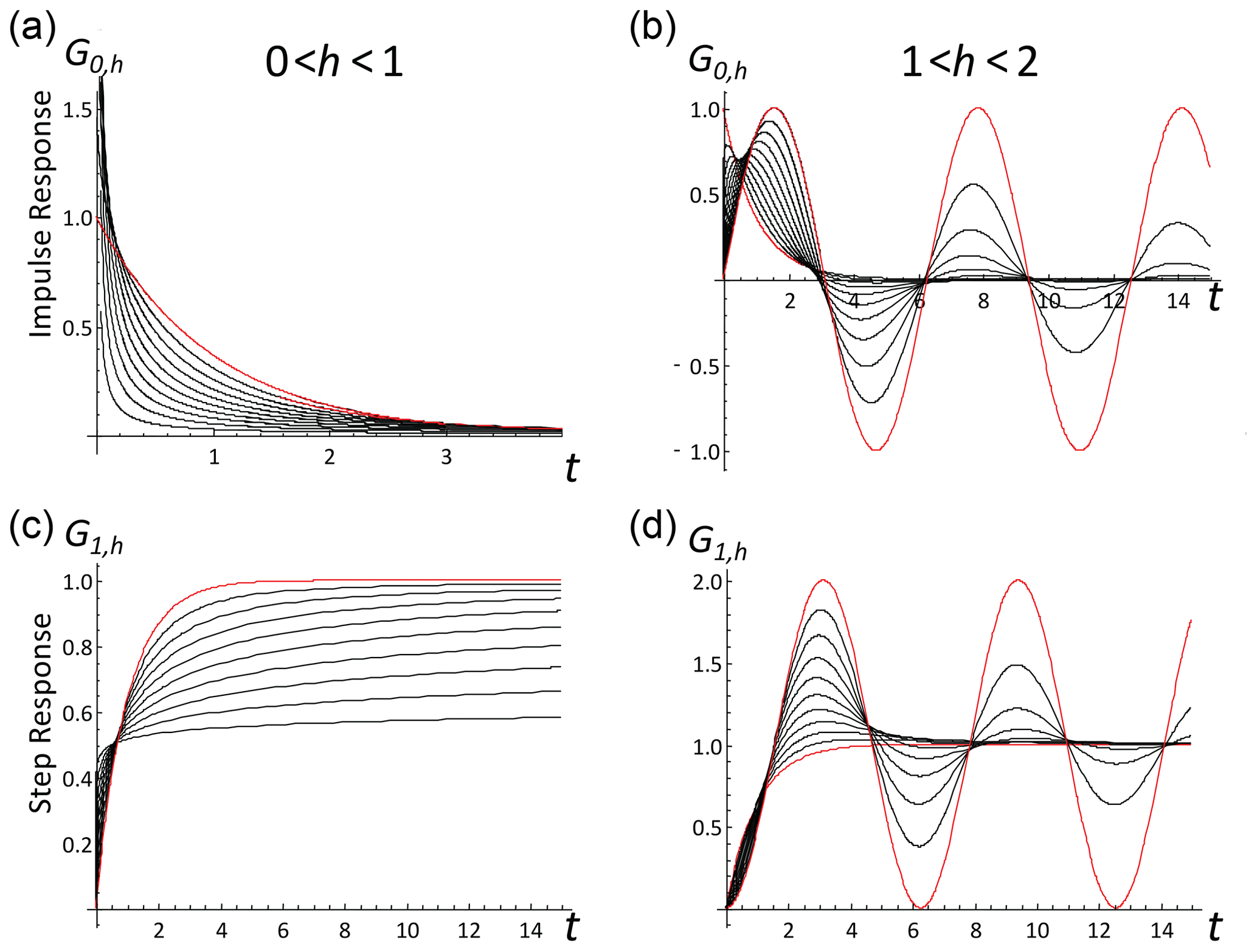
Figure 1The impulse (a, b) and step response functions (c, d) for the fractional relaxation range (a, c: , and red is h=1, the exponential), the black curves, bottom to top, are for , , … and the fractional oscillation range (b, d: , red is the integer values h=1, c, d is the exponential, and a, b h=2), and the sine function, the black curves, bottom to top are for , , …, .
In order to understand the relaxation process – i.e. the approach to the asymptotic value 1 in Fig. 1 for the step response G1,h – we need the asymptotic expansion
For α=0, 1 we obtain the special cases corresponding to impulse and step responses:
(, ; note that the n=0 terms are 0 and 1 for G0,h and G1,h respectively) (Podlubny, 1999), i.e. the asymptotic expansions are power laws in t−h rather than th. According to this, the asymptotic approach to the step function response (bottom row in Fig. 1) is a slow, power law process. In the FEBE, this implies for example that the classical CO2 doubling experiment would yield a power law rather than exponential approach to a new thermodynamic equilibrium. Comparing this to the EBE, i.e. the special case h=1, we have
so that when h=1, the asymptotic step response is instead approached exponentially quickly. We see that when h=1, the process is a classical Ornstein–Uhlenbeck process, so that fRn can be considered a generalization of the latter. There are also analytic formulae for fRn when (the HEBE) is discussed in Appendix B, notably involving logarithmic corrections.
2.3 The α-order fractionally integrated fRn and fRm processes
Before proceeding to discuss the statistics of fRn and fRm processes, it is useful to make a generalization to the fractionally integrated processes:
Uα,h is the “α-order-integrated, fractional h relaxation noise”. Combined with Green's function relation (Eq. 15; recall that for t<0), we find that Uα,h and Gα,h are respectively the fractionally integrated relaxation noises and Green's functions of the fractionally integrated fractional relaxation equation:
If the highest-order derivative is constrained to be an integer (i.e. or 2), then the equation is a standard fractional Langevin equation; for example, U could be for the velocity of a particle with fractional damping and white noise forcing, although even here, the initial conditions are usually taken to be at t=0 and not . Equivalently, Uα,h is the solution of the relaxation equation but with an fGn forcing:
(the Weyl fractional derivatives commute). Fα is the α-order fGn process, and the restriction is needed to ensure low-frequency convergence (see below).
In the Earth's radiative balance, such fractionally integrated fRn processes arise in two physically interesting situations. The first is where the forcing itself has a long memory – e.g. it is an fGn process. Whereas the memory in a pure fRn process is purely from the high-frequency storage term, in this case, the forcing (the overall radiative imbalance) also contributes to the memory, and this has important consequences for the predictability (Sect. 4). Although the solutions Uα,h are mathematically the same whether from the fractional relaxation equation with fGn forcing (Eq. 23) or the fractionally integrated fractional relaxation equation with white noise forcing (Eq. 22), only the former is directly relevant for the Earth's energy balance. This is because the energy balance involves the response from both stochastic (internal) and deterministic (external) forcing. For the latter, it is important that, following a step function forcing, at long times, the system will approach a new state of thermodynamic equilibrium. This implies that the term in the equation that dominates at low frequencies – the lowest-order term – is of order zero, so that if F in Eq. (1) is a step function, the new equilibrium temperature (anomaly) is T=sF.
The second situation where fractionally integrated fRn processes arise is for the energy storage (even in the purely white noise forcing case). The storage process is the difference between the forcing and the response:
so that
Even when the forcing is pure white noise (α=0), the storage is an h-ordered fractionally integrated process: ; this corresponds to the storage following an impulse forcing. The storage following a step forcing is obtained by integration order 1: . Similarly, Green's function for the fRn storage following an impulse forcing is Gh,h and, following a step forcing, (Fig. 2). Since it turns out that most of the pure fRn (α=0) results are readily generalized to , many fractionally integrated results are given below.
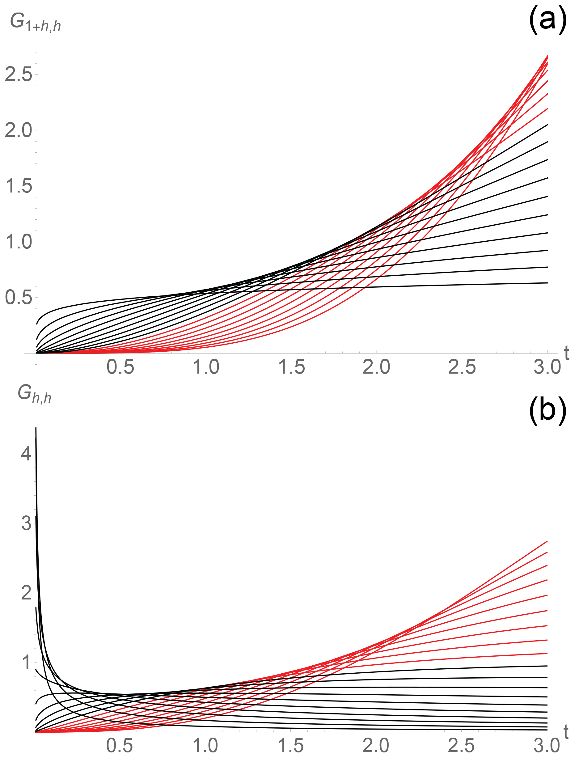
Figure 2The storage Green functions for the fractional relaxation equation (α=0): (a) impulse response (Gh,h); (b) step response (). Black is for , , … and red for , , … (to identify the curves; use the fact that at large t, they are in order of increasing h – bottom to top). For small t, (Eq. 15), so that for , the impulse response is singular at the origin. For large t, (Eq. 18), so that for h<1, the total impulse response storage decreases following the impulse; for h=1 (the EBE), it tends to unity, and for h>1, it diverges.
2.4 Statistics
In the above, we discussed fGn, fRn and their order 1 integrals fBm, fRm as well as fractional generalizations, presenting a classical (real-space) approach stressing the links with fGn and fBm. We now turn to their statistics. Uα,h(t) is a mean zero stationary Gaussian process (i.e. , where “〈.〉” indicates ensemble or statistical averaging); therefore, its statistics are determined completely by its autocorrelation function Rα,h(t), which is only a function of the lag t:
The far-right equality follows from and (“*” indicates “convolution”). The process can only be normalized by Rα,h(0) when there is no small-scale divergence, i.e. when
When , this diverges; in order to be normalized, the process must be averaged at a finite resolution (below).
Although it is possible to follow Mandelbrot and Van Ness (1968) and derive many statistical properties in real space, a Fourier approach is not only more streamlined, but is also more powerful. The reason for the simplicity of the Fourier approach is that the Fourier transform (FT, indicated by the tilde) of the Weyl fractional derivative is symbolically
(e.g. Podlubny, 1999). This is simply the extension of the usual rule for the FT of integer-ordered derivatives. Therefore, since Uα,h and Gα,h are respectively solutions and Green's functions of the fractionally integrated fractional relaxation equation (Eq. 22), we have
so that
We see that in the limit h→0, Uα,0 is an α-order fGn process (see e.g. Eq. 23).
Now we can use the fact that the white noise γ has a flat spectrum:
The modulus (vertical bars) intervenes since for any real function f(t) we have , where the superscript “*” indicates a complex conjugate.
Application of Eq. (31) leads to
i.e. the spectrum EU is the FT of the correlation function Rα,h(t) (the Wiener–Khinchin theorem). Applying this to Uα,h, we obtain
This shows that , so that below, we only consider t≥0.
Since Rα,h(0) diverges for , we consider the integral of the process (the “motion”) from which we can easily compute the average. The corresponding variance Vα,h is
In terms of ,
We see that at low frequencies, when , the integral diverges for all t. Also note that a series expansion for Vα,h(t) in t will only have even-ordered integer power terms.
Comparing Eqs. (33) and (35), we see that R and V are linked by the simple relation
Therefore, by integrating Eq. (26) (twice), we can express Vα,h in terms of Gα,h:
This can be verified by differentiation and using
The basic behaviour can be understood in the Fourier domain. First, putting t=0 in Eq. (32) (i.e. “Parseval's theorem”), we have
so that when , R diverges at high frequencies (small t), and hence to represent a physical process (here, the Earth's temperature), the process must be averaged over a finite-resolution τ. When , R(0) is finite and can therefore be used to obtain a normalized autocorrelation function (Eq. 27).
From Eq. (32), we may also easily obtain the asymptotic high- and low-frequency behaviours of the energy spectrum:
2.5 Finite-resolution processes
When , the process does not converge at any instant t: it is a noise, a generalized function. To represent the Earth's temperature, it must therefore be averaged at a finite-resolution τ:
Applying Eqs. (34) and (40), we obtain the “resolution τ” autocorrelation:
Alternatively, measuring time in units of the resolution ,
can be conveniently written in terms of centred finite differences:
The finite-difference formula is valid for Δt≥τ. For finite τ, it allows us to obtain the correlation behaviour by replacing the second difference with a second derivative, an approximation that is very good except when Δt is close to τ. Taking the limit τ→0 in Eq. (43), we obtain the second derivative formula Eq. (36).
3.1 fBm and fGn
The above derivations were for noises and motions derived from differential operators whose impulse and step Green functions had convergent Vα,h(t). Before applying them to fRn and fRm, we illustrate this by applying them first to fBm and fGn.
The fBm results are obtained by using the fGn step Green function (Eq. 13) in Eq. (35) with h=0 to obtain
The standard normalization and parametrization are
This normalization turns out to be convenient not only for fBm, but also for fRm, so that for the normalized process,
where we have introduced the standard fBm parameter , so that
and hence H is the fluctuation exponent for fBm. Note that fBm is usually defined as the Gaussian process with VH given by Eq. (46), i.e. with this normalization (e.g. Biagini et al., 2008).
We can now calculate the correlation function relevant for the fGn statistics. With the above normalization,
the bottom approximations are valid for large-scale ratios λ. We note the difference in sign for (“persistence”) and for (“anti-persistence”). When , the noise corresponds to standard Brownian motion, and it is uncorrelated.
3.2 fRm and fRn
3.2.1 Rα,h(t)
Since fRm and fRn are Gaussian, their properties are determined by their second-order statistics, by Vα,h(t) and Rα,h(t). These statistics are second order in Gα,h(t) and can most easily be determined using the Fourier representation of Gα,h(t) (Sect. 2.4, Appendices A and B). The development is challenging because unlike the Gα,h(t) functions that are entirely expressed in series of fractional powers of t, Vα,h(t) and Rα,h(t) involve mixed fractional and integer power expansions; the details are given in the Appendices, and here we summarize the main results.
First, for the noises, we have
At small t, the lowest-order terms dominate, and the normalized autocorrelations are thus
(note that F3<0 for ; see Appendix A). We see that at small t, the behaviour of the normalized autocorrelations depends essentially on the sum h+α; in particular, when , the process is effectively an fGn process with an effective fluctuation exponent . This is to be expected since α+h is the highest-order term in the fractionally integrated fractional relaxation equation (Eq. 22).
3.2.2 Vα,h(t)
Integrating twice
we obtain
When , the leading (n=2) term for Vα,h is (), so that the fBm coefficient can be used for normalization using . When , this normalization becomes negative, so that it cannot be used; however, in this case, and may be used for normalization instead. For an analytic expression, convergence properties including numerical results and modified expansions converge more rapidly; see Appendix A and, for the special case , Appendix B.
For convenience, the leading terms of the normalized Vα,h are
3.2.3 Asymptotic expansions
For multidecadal global climate projections, the relaxation time has been estimated at ≈ 5 years (Procyk et al., 2020, 2022), so that we are interested in the long-time behaviour (exploited for example in Hébert et al., 2021). For this, asymptotic expansions are needed: in Appendix A we show
where for h<1, while for it has exponentially damped oscillations (see Fig. 3d and Appendix A).
Figure 3The normalized correlation functions R0,h for fRn corresponding to the V0,h function in Fig. 4: (a), (b), (c), and (d). In each plot, the curves correspond to h increasing from bottom to top in units of starting from (a) to (d). For , the resolution is important since diverges at small τ. In (a), is shown with ; they were normalized to the value at resolution , and for , the curves are normalized with . In all cases, the large t slope is .
For pure fRn processes, a useful formula is
or, more generally,
We see that when α≠0, D0>0, so that, as expected, the leading behaviour has no h dependence: it is only due to the long-range correlations in the forcing; we obtain the fGn result: . For pure fRn processes this reduces to
(note that for ).
Integrating Rα,h twice and doubling, we obtain
(the full expansion is given in Appendix A; see Fig. 4 for plots). The constants of integration aα,h and bα,h are not determined since the expansion is not valid at t=0; they can be determined numerically if needed. However, in the limit α→0 (the pure fRn case), the leading term is exactly t (corresponding to ordinary Brownian motion), so that an extra a0,h is not needed (Appendix A). When α>0, the far-left (fGn) term from the forcing dominates; at large enough t, with , and the corresponding motion is an fBm.
Figure 4The normalized V0,h functions for the various ranges of h for fRm. The plots from (a) to (d) are for the ranges , , , and . Within each plot, the lines are for h increasing in units of starting at a value above the plot minimum; overall, h increases in units of starting at values (a) to (d) (e.g. for a, the lines are for , , , , and ). For all h the large t behaviour is linear (slope =1, although note the oscillations for the lower right-hand plot (d) for ). For small t, the slopes are 1+2h () and 2 ().
Using the above results, we see that there are three limiting fRnfRm cases that yield fGnfBm processes:
3.3 Haar fluctuations
A useful statistical characterization of the processes is by the statistics of their Haar fluctuations over an interval Δt. For an interval Δt, Haar fluctuations (based on Haar wavelets) are the differences between the averages of the first and second halves of an interval. For a process U, the Haar fluctuation is
In terms of the process at resolution (i.e. averaged at this scale), :
Therefore,
where V(t) is the variance of the integral of U over an interval t (Eq. 34).
Using Eq. (60), we can determine the behaviour of the root mean square (rms) Haar fluctuations; terms like contribute to the rms Haar fluctuation (the exception is when ξ=2, which contributes nothing). Applying this equation to fGn parameter h, we obtain with .
Using the results above for Vα,h, we therefore obtain the leading exponents:
Figure 5 shows that the theory agrees well with the numerics.
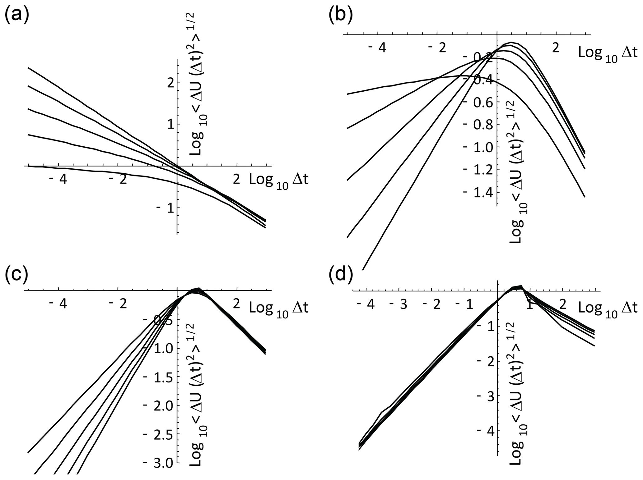
Figure 5The rms Haar fluctuation plots for the pure (α=0) fRn process for (a), (b), (c), and (d). The individual curves correspond to those of Figs. 3 and 4. The small Δt slopes follow the theoretical values up to (slope=1); for larger h, the small t slopes all equal 1. Also, at large t due to dominant V≈t terms, in all cases we obtain slopes .
For the range of α, h discussed here (, ), H spans the range (white noise) to 1. In comparison, fGn processes have H covering the range and fBm processes have ; therefore, depending on whether the process is observed at timescales below or above the relaxation timescale (Δt=1), fractionally integrated fRn processes can mimic fGn or fBm processes. If we consider the integrals – the motions – the value of H is increased by 1 (although for Haar fluctuations, it cannot exceed H=1). Overall, from an empirical viewpoint, if over some range of scales (that may only be a factor of 100 or less), it may be quite hard to distinguish the various models, especially since the transition from low- to high-frequency scaling may be very slow (see especially Appendix B for the case). Recent work shows that the maximum likelihood method may be the optimum parameter estimation technique (Procyk, 2021).
3.4 Sample processes
It is instructive to view some samples of fRn and fRm processes (here we consider only α=0). For simulations, both the small- and large-scale divergences must be considered. Starting with the approximate methods developed by Mandelbrot and Wallis (1969), it took some time for exact fBm and fGn simulation techniques to be developed (Hipel and McLeod, 1994; Palma, 2007). Fortunately, for fRm and fRn, the low-frequency situation is easier since the long-time memory is much smaller than for fBm and fGn. Therefore, as long as we are careful to always simulate series a few times longer than the relaxation time and then to throw away the earliest or of the simulation, the remainder will have accurate statistics. With this procedure to take care of low-frequency issues, we can therefore use the solution for fRn in the form of a convolution and use standard numerical convolution algorithms.
We must nevertheless be careful about the high frequencies since the impulse response Green functions G0,h are singular for h<1. In order to avoid singularities, simulations of fRn are best made by first simulating the motions Q0,h using and obtaining the resolution τ fRn, using . Numerically, this allows us to use the smoother (nonsingular) G1,h in the convolution rather than the singular G0,h. The simulations shown in Figs. 6–9 follow this procedure, and the Haar fluctuation statistics were analysed, verifying the statistical accuracy of the simulations.
In order to clearly display the behaviours, recall that when t≫1, we showed that all the fRn converge to Gaussian white noises and the fRm to Brownian motions (albeit in a slow power law manner). At the other extreme, for t≪1, we obtain the fGn and fBm limits (when ) and their generalizations for .
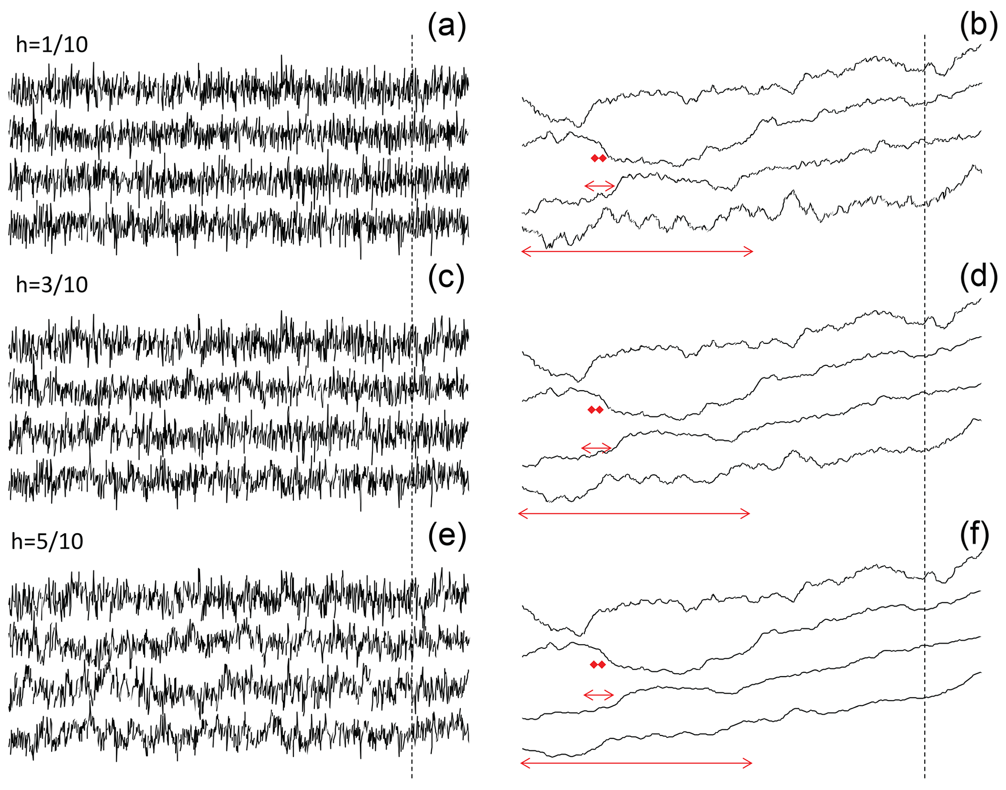
Figure 6fRn and fRm simulations (left and right columns respectively) for , , and (top to bottom sets, all with α=0), i.e. the exponent range that overlaps with fGn and fBm. There are three simulations, each of length 219 pixels, and each uses the same random seed with the unit scale equal to 210 pixels (i.e. a resolution of ). The entire simulation therefore covers the range of scale to 512 units. The fRm on the right is from the running sum of the fRn on the left. Starting at the top line of each set, we show 210 points of the original series degraded in resolution by a factor 29. Since the length is t=29 units long, each pixel has resolution . The second line of each set takes the segment of the upper line lying to the right of the dashed vertical line, of its length. It therefore spans t=0 to , but resolution was taken as , and hence it is still 210 pixels long. Since each pixel has a resolution of 2−4, the unit scale is 24 pixels long: this is shown in red in the second series from the top (middle set). The process of taking and blowing up by a factor of 8 continues to the third line (length t=23, resolution ), unit scale=27 pixels (shown by the red arrows in the third series), until the bottom series which spans the range t=0 to t=1, and resolution with unit scale 210 pixels (the whole series displayed). Each series was rescaled in the vertical so that its range between maximum and minimum was the same. The unit relaxation scales indicated by the red arrows mark the transition from small to large scales. Since the top series in each set has a unit scale of 2 (degraded), it is nearly a white noise (a, c, e) or (ordinary) Brownian motion (b, d, f). In contrast, the bottom series is exactly of length t=1, so that it is close to the fGn and fBm limits (left and right) with the standard exponent . As indicated in the text, the second series from the top in the bottom set is most realistic for monthly temperature anomalies.
Figure 6 shows three simulations, each of length 219 pixels, with each pixel corresponding to a temporal resolution of , so that the unit (relaxation) scale is 210 elementary pixels. Each simulation uses the same random seed, but they have h's increasing from (top set) to (bottom set). The fRm on the right is from the running sum of the fRn on the left. Each series has been rescaled, so that the range (maximum–minimum) is the same for each. Starting at the top line of each group, we show 210 points of the original series degraded by a factor of 29. The second line shows a blow-up by a factor of 8 of the part of the upper line to the right of the dashed vertical line. The line below is a further blow-up by a factor of 8 until the bottom line shows a part of the full simulation but at full resolution. The unit scale indicating the transition from small to large is shown by the horizontal red line in the middle-right figure. At the top (degraded by a factor of 29), the unit (relaxation) scale is 2 pixels, so that the top line degraded view of the simulation is nearly a white noise (left) or (ordinary) Brownian motion (right). In contrast, the bottom series is exactly of length unity, so that it is close to the fGn limit with the standard exponent . Moving from bottom to top in Fig. 6, one effectively transitions from fGn to fRn (left column) and from fBm to fRm (right column).
If we take the empirical relaxation scale for the global temperature to be 27 months (≈10 years, Lovejoy et al., 2017) and we use monthly-resolution temperature anomaly data, then the nondimensional resolution is 2−7, corresponding to the second series from the top (which is thus 210 months ≈80 years long). Since (Procyk et al., 2022), the second series from the top in the bottom set is the most realistic, and we can make out the low-frequency undulations that are mostly present at scales of the series (or less).
Figure 7 shows realizations constructed from the same random seed but for the extended range (i.e. beyond fGn). Over this range, the top (large-scale, degraded-resolution) series are close to white noises (left) and Brownian motions (right). For the bottom series, there is no equivalent fGn or fBm process and the curves become smoother, although the rescaling may hide this somewhat (see for example the set, the blow-up of the far-right of the second series from the top shown in the third line). For , also note the oscillations with frequency (Eqs. 53 and A3): this is the fractional oscillation range.
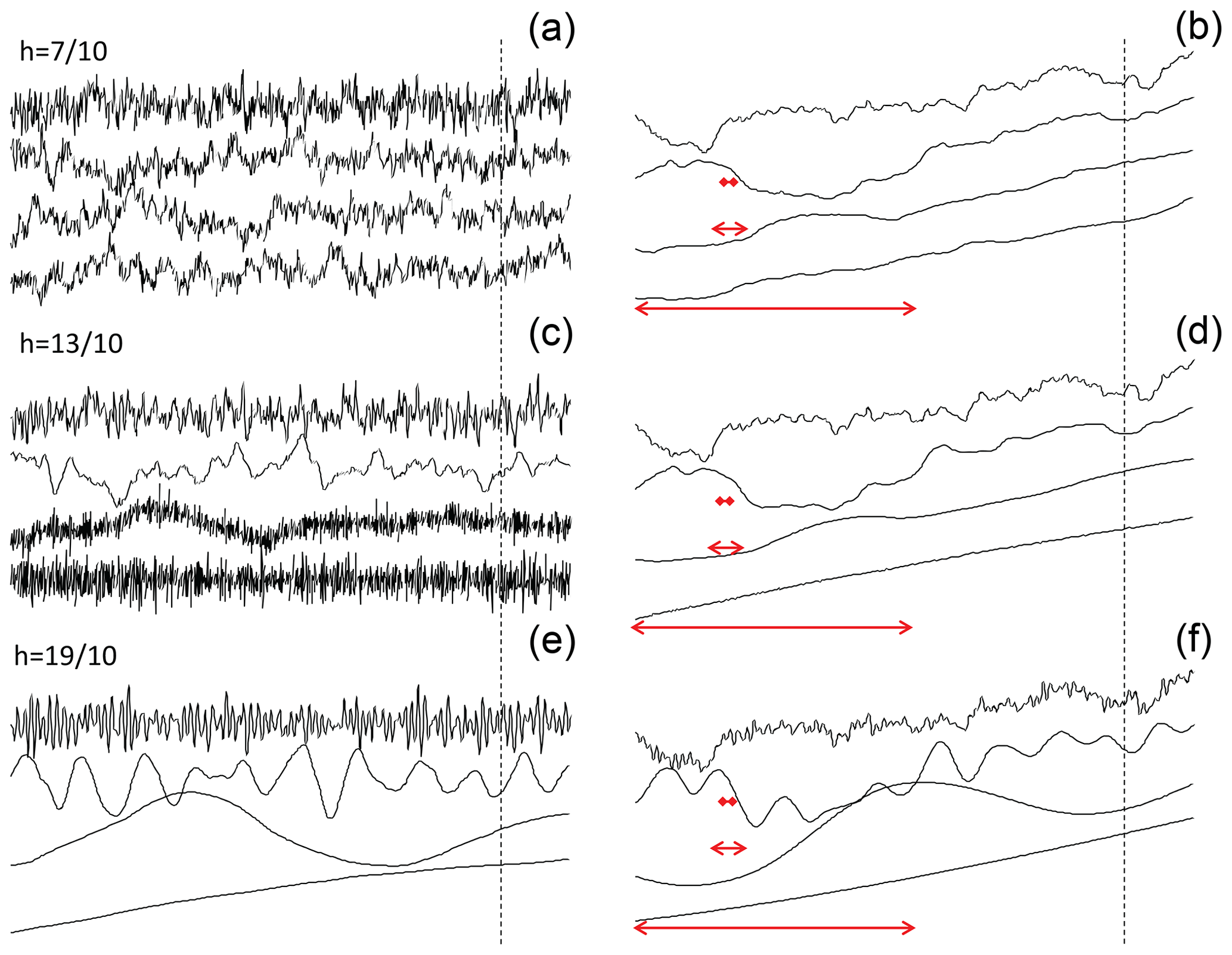
Figure 7The same as Fig. 6 but for , and (top to bottom). Over this range, the top (large-scale, degraded-resolution) series is close to a white noise (a, c, e) and Brownian motion (b, d, f). For the bottom series, there is no equivalent fGn or fBm process and the curves become smoother, although the rescaling may hide this somewhat (see for example the middle set, the blow-up of the far-right of the second series from the top shown in the third line). Also note for the bottom two sets with the oscillations that have frequency : this is the fractional oscillation range.
Figure 8 shows simulations similar to Fig. 5a (fRn on the left, fRm on the right), except that instead of making a large simulation and then degrading and zooming, all the simulations were of equal length (210 points), but the relaxation scale was changed from 215 pixels (bottom) to 210, 25 and 1 pixel (top). Again, the top is white noise (left) and Brownian motion (right), and the bottom is (nearly) fGn (left) and fBm (right); Fig. 9 shows the extensions to .
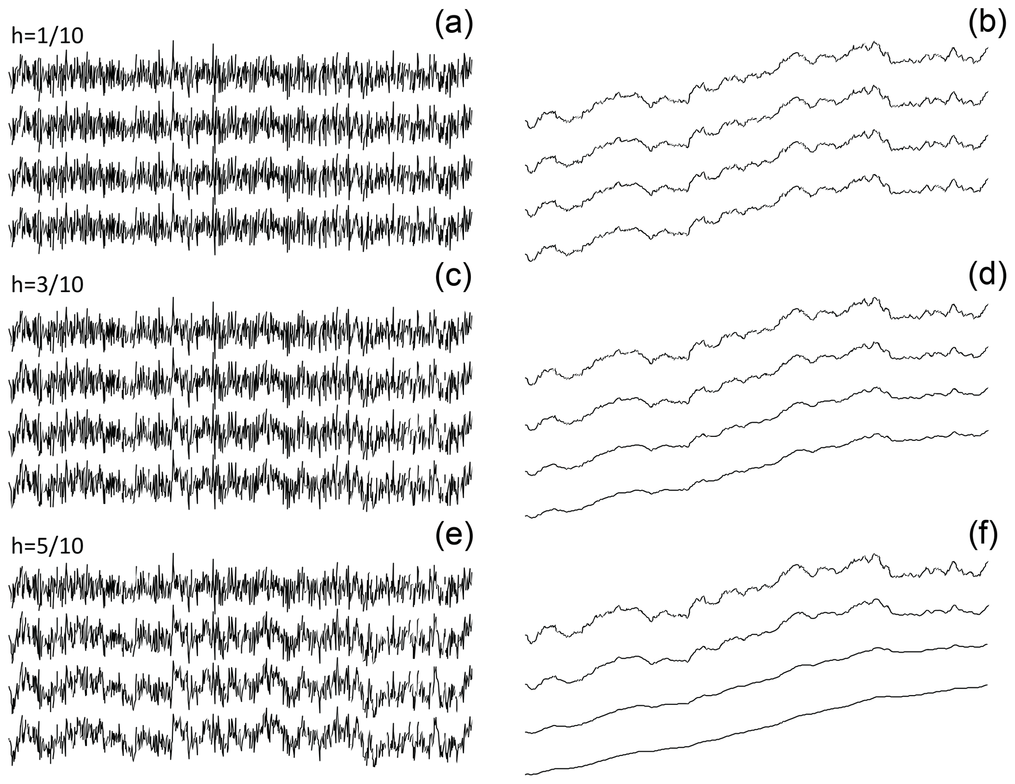
Figure 8This set of simulations is similar to Fig. 6 ((a, c, e) fRn, (b, d, f) fRm) except that instead of making a large simulation and then degrading and zooming, all the simulations were of equal length (210 points) but resolutions , 2−10, 2−5, and 1 (bottom to top). The simulations therefore spanned the ranges of scale 2−15 to 2−5, 2−10 to 1, 2−5 to 25, and 1 to 210, and the same random seed was used in each so that we can see how the structures slowly change when the relaxation scale changes. The bottom fRn, set is the closest to that observed for the Earth's temperature, and since the relaxation scale is of the order of a few years, the second series from the top of this set (with 1 pixel = 1 month) is close to that of monthly global temperature anomaly series. In that case the relaxation scale would be 32 months and the entire series would be years long. The top series (of total length 210 relaxation times) is (nearly) a white noise (a, c, e) and Brownian motion (b, d, f), and the bottom is (nearly) an fGn (a, c, e) and fBm (b, d, f). The total range of scales covered here (210×215) is larger than in Fig. 5a and allows one to more clearly distinguish the high- and low-frequency regimes.

The initial value for Weyl fractional differential equations is effectively at , so that for fRn, it is not directly relevant at finite times (although the ensemble mean is assumed=0; for fRm, the initial condition is important). The prediction problem is thus to use past data (say, for t<0) in order to make the most skillful prediction for t>0. We are therefore dealing with a past value rather than usual initial value problem. The emphasis on past values is particularly appropriate since in the fGn limit, the memory is so large that values of the series in the distant past are important. Indeed, prediction of fGn with a finite length of past data involves placing strong (mathematically singular) weight on the most ancient data available (see Gripenberg and Norros, 1996; Del Rio Amador and Lovejoy, 2019, 2021a, b). This is quite different from standard stochastic predictions that are based on short-memory (exponential) auto-regressive or moving-average-type processes that are not much different from initial value problems.
To deal with the small-scale divergences when , it is necessary to predict the finite-resolution fRn: . Using Eq. (40) for , we have
Now define the predictor for t≥0 (indicated by a circumflex):
To show that it is indeed the optimal predictor, consider the predictor error Eτ(t):
Equation (64) shows that the error depends only on γ(v) for v>0, whereas the predictor (Eq. 63) only depends on γ(v) for v<0, and hence they are orthogonal:
This is a sufficient condition for to be the minimum square predictor, which is the optimal predictor for stationary Gaussian processes (e.g. Papoulis, 1965). The prediction error variance is
or, with a change in variables,
where we have used (the unconditional variance).
There are numerous skill indicators, but the most popular and easy-to-interpret definition of forecast skill is the minimum square skill score or MSSS (Sk,τ, see Del Rio Amador and Lovejoy, 2021a, for a discussion of this and other indicators). For this, we obtain
When and
we obtain the fGn result:
(Lovejoy et al., 2015), where λ is the forecast horizon (lead time) measured in the number of time steps in the future (due to the fGn scaling, it is independent of the resolution τ). The MSSS gives the fraction of the variance explained by the optimum predictor; when skill=1, the forecast is perfect.
To survey the implications, let us start by showing the τ independent results for fGn, shown in Fig. 10, which is a variant on a plot published in Lovejoy et al. (2015). We see that when (H≈1), the skill is very high; indeed, in the limit , we have perfect skill for fGn forecasts (this would of course require an infinite amount of past data to attain).
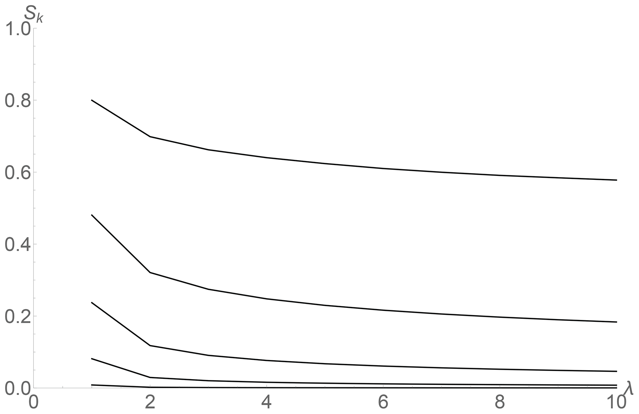
Figure 10The prediction skill (Sk) for pure fGn processes for forecast horizons up to λ=10 steps (10 times the resolution). This plot is nondimensional, and it is valid for time steps of any duration. From bottom to top, the curves correspond to , , … (red, top, close to the empirical h).
Now consider the fRn skill: we will start by considering the pure (α=0) fRn case where the memory comes completely from the (high-frequency) storage, anticipating that the fGn forced case (α≠0) obtains its memory and skill from both storage and forcing. In comparison with fGn, fRn has an extra parameter, the resolution of the data, τ. Figure 11 shows curves corresponding to Fig. 10 for fRn with forecast horizon integer multiples (λ) of τ, i.e. for times t=λτ in the future but with separate curves, one for each of five τ values increasing from 10−4 to 10 by factors of 10. When τ is small, the results should be close to those of fGn, i.e. with potentially high skill, and in all cases, the skill is expected to vanish quite rapidly for τ>1 since in this limit, fRn becomes an (unpredictable) white noise (although there are scaling corrections to this).

Figure 11Panels (a, c, e) show the skill (Sk) of pure (α=0) fRn forecasts (as in Fig. 10 for fGn) for fRn skill with , , and (top to bottom sets); λ is the forecast horizon, the number of steps of resolution τ forecast into the future. Panels (b, d, f) show the ratio (r) of the fRn to the corresponding fGn skill. Here the result depends on τ; each curve is for different values increasing from 10−4 (top, black) to 10 (bottom, purple) and increasing by a factor of 10 (the red set in the bottom plots with ; are closest to the empirical values).
To better understand the fGn limit, it is helpful to plot the ratio of the fRn-to-fGn skill (Fig. 11, right column). We see even with quite small values (top, black curves) that some skill has already been lost. Figure 12 shows this more clearly: it shows 1-time-step and 10-time-step skill ratios. To put this into perspective, it is helpful to compare this using some of the parameters relevant to macroweather forecasting. According to Lovejoy et al. (2015) and Del Rio Amador and Lovejoy (2019), the relevant empirical Haar exponent is for the global temperature, so that . Although direct empirical estimates of the relaxation time are difficult since the responses to anthropogenic forcing begin to dominate over the internal variability after ≈10 years, Procyk et al. (2022) have used the deterministic response to estimate a global relaxation time of ≈5 years (work in progress using maximum likelihood estimates shows that at scales of hundreds of kilometres, it is quite variable, ranging from months to decades; Procyk, 2021). For monthly-resolution forecasts, the nondimensional resolution is . With these values, we see (red curves) that we may have lost ≈30 % of the fGn skill for 1-month forecasts and ≈85 % for 10-month forecasts. Comparing this with Fig. 10, we see that this implies about 60 % and 10 % skill (see also the red curve in Fig. 11, bottom set).
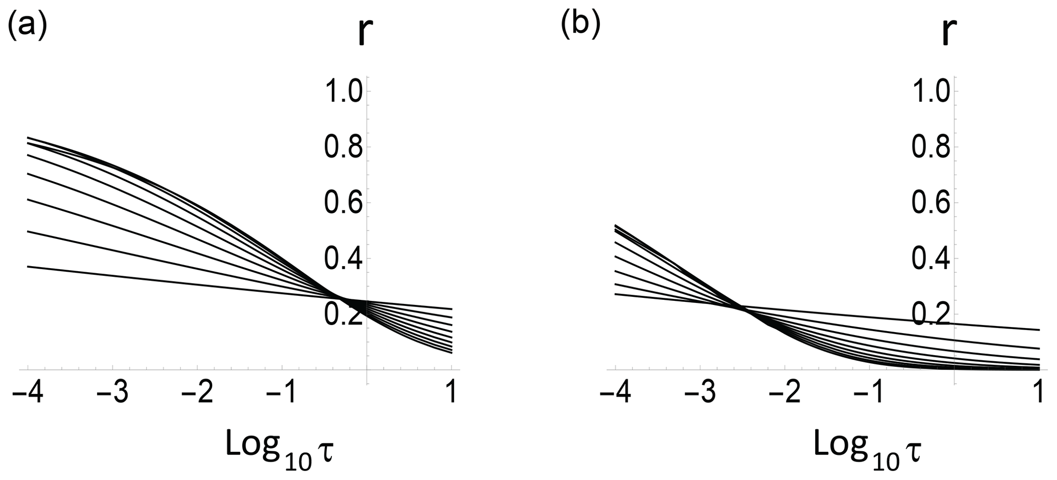
Figure 12The ratio of (α=0) fRn skill to fGn skill (a: 1-step horizon, b: 10-step forecast horizon) as a function of resolution τ for h increasing from (at left) bottom to top (, , … ); the curve (close to the empirical value) is the curve that starts at the upper left of each plot.
Going beyond the region that overlaps fGn, Figs. 12 and 13 clearly show that the skill continues to increase with h. We already saw (Fig. 4) that the range has rms Haar fluctuations that for Δt<0 mimic fBm, and these do indeed have higher skill, approaching unity for h near 1 corresponding to a Haar exponent , i.e. close to an fBm with , i.e. a regular Brownian motion. Recall that for Brownian motion, the increments are unpredictable but the process itself is predictable (persistence). In Fig. 12, we show the skill for various h's as a function of resolution τ. Figure 14 shows that for , the skill decreases rapidly for τ>1. Figure 15 in the fractional oscillation equation regime shows that the skill oscillates.

Figure 13The 1-step (a) and 10-step (b) pure (α=0) fRn forecast skill as a function of h for various resolutions (τ) ranging from (black, left of each set) through (brown) 10−2 (red), 0.1 (blue), 1 (orange), and 10 (purple). In the right set τ=1 (orange), 10 (purple) lines are nearly on top of the Sk=0 line. Again, red () is the more empirically relevant value for monthly data. Recall that the regime (to the left of the vertical dashed lines) corresponds to the overlap with fGn.

Figure 14One-step pure (α=0) fRn prediction skills as a function of resolution for hs increasing from (bottom) to (top) every . Note the rapid transition to low skill (white noise) for τ>1. The curve for is shown in red.
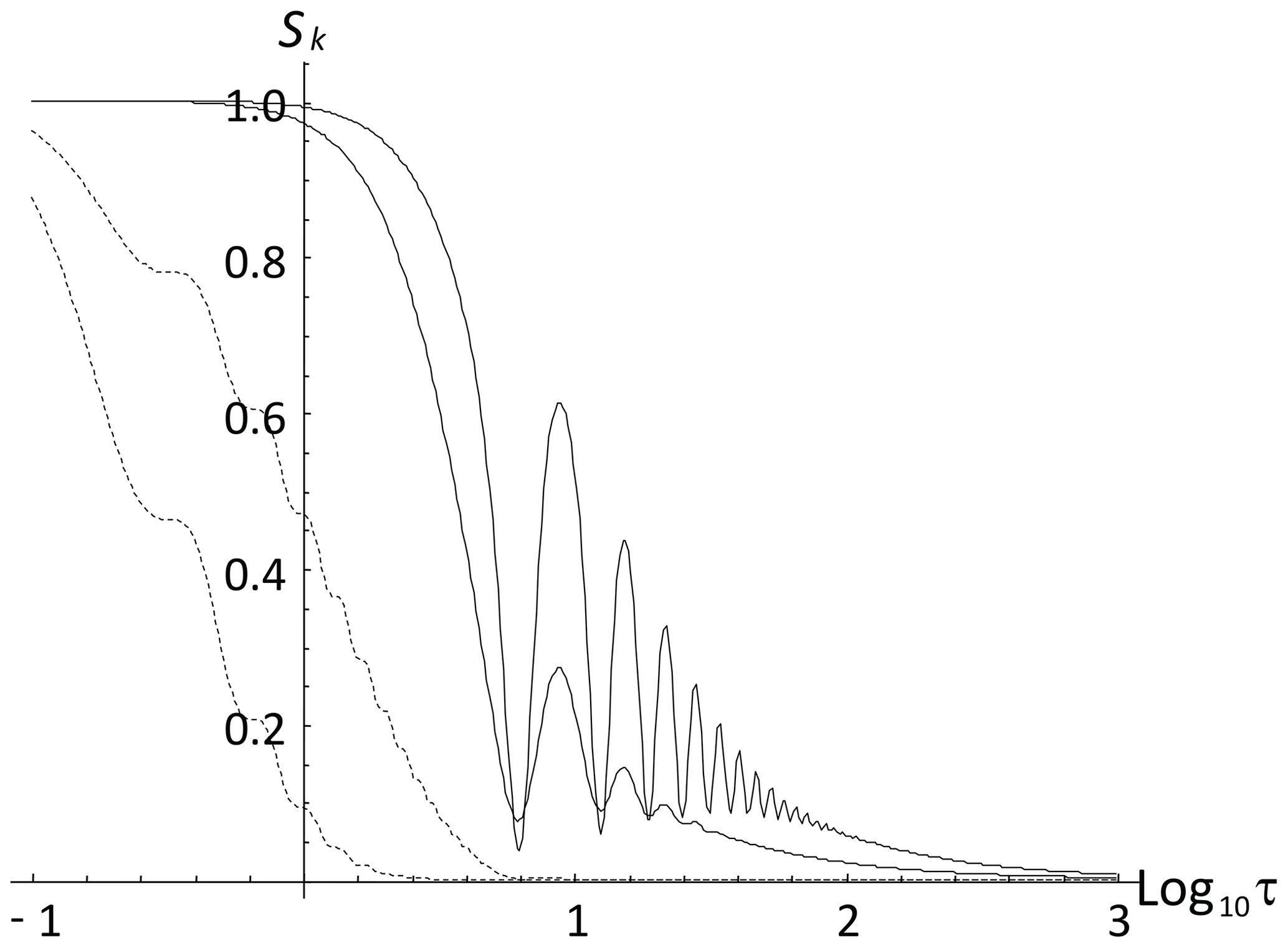
Figure 15Same as Fig. 14 except for and showing the 1-step skill (black) and 10-step skill (dashed). The right-hand dashed and right-hand solid lines are for : they clearly show that the skill oscillates in this fractional oscillation equation regime. The corresponding left lines are for .
We may now consider the skill of the fGn-forced process (α≠0) in Fig. 16. For small τ, short lags, λ (the upper left), the contours are fairly linear along lines of constant h+α, so that, as expected, the predictability is essentially that of an fGn process but with an effective exponent h+α. At the opposite extreme, (large τ, h) the lines are fairly horizontal, indicating that the skill from the storage (i.e. from h) is negligible and that all the memory (and hence skill) comes from the forcing fGn, exponent α. The in-between resolutions and lags generally have in-between slopes. As expected, the skill from the storage drops off quickly for resolutions . For h≥1, there is some waviness in the contours due to the oscillatory nature of the Green functions.

Figure 16Contour plots of the forecast skill, with h along the horizontal axis and α along the vertical axis. The plots are for increasing nondimensional resolutions: τ=0.001, 0.01, 0.1, 1, and 10 (top to bottom), with forecasts for lags λ=1, 3, and 10 (left to right) and with contour levels (legend) varying from nearly no skill (0.03) to nearly full skill (0.98).
Ever since Budyko (1969) and Sellers (1969), the energy balance between the Earth and outer space has been modelled by the energy balance equation (EBE) based on the continuum heat equation; see North and Kim (2017) for a recent review and see Ziegler and Rehfeld (2020) for a recent regional application. It is most commonly used as a model for the globally averaged temperature, where it is usually derived by applying Newton's law of cooling applied to a uniform slab of material, a “box”. The resulting EBE is a first-order relaxation equation describing the exponential relaxation of the temperature to a new equilibrium after it has been perturbed by an external forcing. Its first-order (h=1) derivative term accounts for energy storage.
The resulting model relaxes to equilibrium much too quickly, so that to increase realism, it is usual to introduce a few interacting slabs (representing for example the atmosphere and ocean mixed layer; the Intergovernmental Panel on Climate Change recommends two such components; IPCC, 2013). However, it turns out that these h=1 box models do not use the correct surface radiative–conductive boundary conditions. If one assumes heat transport by the classical heat equation and radiative–conductive boundary conditions are used instead, one instead obtains the half-order EBE, the HEBE with (Lovejoy, 2021a, b), which is already close to the global empirical value (, Procyk et al., 2022; Del Rio Amador and Lovejoy, 2019; see also Lovejoy et al., 2015). However, this model is only valid in the macroweather regime – for timescales of weeks and longer and, due to the spatial scaling in the atmosphere, the fractional heat equation (FHE) may be a more appropriate model than the classical one. The use of the FHE can be justified by recognizing that a realistic energy transport model involves a continuous hierarchy of mechanisms. The extension to the FHE leads directly to a fractional relaxation equation that generalizes the EBE: the fractional energy balance equation (Lovejoy, 2021a, b) (FEBE). The FEBE can also be derived phenomenologically by assuming that energy storage processes are scaling (Lovejoy, 2019; Lovejoy et al., 2021).
When forced by a Gaussian white noise, the FEBE is also a generalization of fractional Gaussian noise (fGn), and its integral (fractional relaxation motion, fRm) generalizes fractional Brownian motion (fBm). More classically, it generalizes the Orenstein–Uhlenbeck process that corresponds to the h=1 special case (i.e. the standard EBE with white noise forcing). Over the parameter range , the high-frequency FEBE limit (fGn) has been used as the basis of monthly and seasonal temperature forecasts (Lovejoy et al., 2015; Del Rio Amador and Lovejoy, 2019, 2021a, b); at 1-month lead times, these macroweather forecasts are similar in skill to conventional numerical models, whereas for bimonthly, seasonal and annual forecasts, they are more skillful (Del Rio Amador and Lovejoy, 2021a). For multidecadal timescales the low-frequency limit has been used as the basis of climate projections through to the year 2100 (Hébert, 2017; Lovejoy et al., 2017; Hébert et al., 2021), and more recently, the full FEBE has been used directly (Procyk et al., 2020, 2022; Procyk, 2021).
It was the success of predictions and projections with different exponents but the same theoretically derived empirical underlying FEBE h≈0.4 that, over recent years, motivated the development of the FEBE (announced in Lovejoy, 2019) and the work reported here. The statistical characterizations, correlations, structure functions, Haar fluctuations and spectra as well as the predictability properties are important for these and other FEBE applications and are derived in this paper.
While the deterministic fractional relaxation equation is classical, various technical difficulties arise when it is generalized to the stochastic case: in the physics literature, it is a fractional Langevin equation (FLE) that has almost exclusively been considered a model of diffusion of particles starting at an origin. This requires t=0 initial conditions that imply that the solutions are strongly nonstationary. In comparison, the Earth's temperature fluctuations that are associated with its internal variability are statistically stationary. This can easily be modelled with initial conditions at , i.e. by using Weyl fractional derivatives. In addition, in the usual FLE, the highest-order derivative is an integer, so that sample processes are rms differentiable of order at least 1 (Watkins et al., 2020, have called the FEBE a “Fractionally Integrated FLE”). In the FEBE and the fractionally integrated extensions, the highest-order derivative is readily of order , so that sample processes are generalized functions (“noises”) and must be smoothed/averaged for physical applications.
Although EBEs were originally developed to understand the deterministic temperature response to external forcing, the temperature also responds to stochastic “internal” forcing. While the Earth's system variability is generally highly non-Gaussian (multifractal, Lovejoy, 2018), the temporal macroweather regime modelled here is the quasi-Gaussian exception. This paper therefore explores the statistics of the temperature response when it is stochastically forced by Gaussian processes, both by white noise (α=0) and by a (long-memory) fractional Gaussian noise (fGn) process. The white noise special case – “pure fRn and fRm” – is the α=0 special case; the fGn-forced case extends the parameter range to . According to work in progress using satellite and reanalysis radiances, both cases appear to be empirically relevant for modelling the Earth's energy balance.
A key novelty is therefore to consider the fractional relaxation equation (a FLE) forced by white and scaling noises starting from , equivalent to Weyl's “fractionally integrated fractional relaxation equation”. In addition, the highest-order terms in standard FLEs are integer-ordered: the fractional terms represent damping and are of lower order, guaranteeing that solutions are regular functions. However, the FEBE's highest-order term is fractional, and over the main empirically significant parameter range () the processes are noises (generalized functions): in order to represent physical processes, they must be averaged. This is conveniently handled by introducing their integrals or “motions”. We proceeded to derive their fundamental statistical properties, including series expansions about the origin and infinity. These expansions are nontrivial since they mix fractional and integer-ordered terms (Appendix A). Since the FEBE is used as the basis for macroweather predictions, the theoretical predictability skill is important in applications and was also derived.
With these stationary Gaussian forcings, the solutions are a new stationary process – fRn (α=0) and its extensions to fractionally integrated fRn processes (α>0). Over the range , we show that the small-scale limit is an fGn, and its integral – fRm – has stationary increments and generalizes fBm. Although at long enough times the fRn (α=0) tends to a Gaussian white noise and fRm to a standard Brownian motion, this long time convergence is typically very slow (when α>0, the long time behaviours are fGn and fBm processes, parameter α).
Much of the effort was in deducing the asymptotic small- and large-scale behaviours of the autocorrelation functions that determine the statistics and in verifying these with extensive numerical simulations. An interesting exception was the special case, which for fGn corresponds to an exactly noise. Here, we give the exact mathematical expressions for the full correlation functions, showing that they had logarithmic dependencies at both small and large scales. The resulting HEBE has an exceptionally slow transition from small to large scales (a factor of a million or more is needed), and empirically it is quite close to the global temperature series over scales of months, decades and possibly longer.
Beyond improved monthly and seasonal temperature forecasts and multidecadal projections, the stochastic FEBE opens up several paths for future research. One of the more promising is to apply these techniques to the spatial FEBE and generalize it in various directions. This is a follow-up on the special value that is very close to that found empirically and that can be analytically deduced from the classical Budyko–Sellers energy transport equation by improving the mathematical treatment of the radiative boundary conditions (Lovejoy, 2021a, b). In the latter case, one obtains a partial fractional differential equation for the horizontal space–time variability of temperature anomalies over the Earth's surface, allowing regional forecasts and projections. This has already allowed improved regional projections (Procyk, 2021) and promises better monthly and seasonal forecasts.
While the FEBE has already demonstrated its ability to project future climates, these improvements will allow for the modelling of the nonlinear albedo–temperature feedbacks needed for modelling of transitions between different past climates. Finally, FEBE-based projections have shown that, in spite of improved computer power and algorithms, conventional GCM approaches may be suffering from diminishing returns; the GCMs in the latest IPCC assessment (AR6, 2021) are even more uncertain: a range of 2–5.5 KCO2 doubling (90 % confidence) those in the previous assessment (AR5, 2013, 1.5–4.5 K per doubling) while also being somewhat warmer. The FEBE had the somewhat lower but much less uncertain range 1.6–2.4 KCO2 doubling (90 % confidence). Conventional GCM approaches attempt to explicitly model as many degrees of freedom as possible, and by the year 2030 they are expected to have kilometric-scale (“cloud-resolving”) resolutions that will model structures that live for only 15 min and then average them over decades. The FEBE (with regional and other future extensions) is, in contrast, a high-level stochastic model that accounts for the collective interactions of huge numbers of degrees of freedom (Lovejoy, 2019). It is thus a promising candidate for a new generation of climate models.
A1 Rα,h(t) as a Laplace transform
In Sect. 2.4, we derived general statistical formulae for the autocorrelation functions of motions and noises defined in terms of Green's functions of fractional operators. Since the processes are Gaussian, autocorrelations fully determine the statistics. While the autocorrelations of fBm and fGn are well known, those for fRm and fRn are new and are not so easy to deal with since they involve quadratic integrals of Mittag–Leffler functions. In this Appendix, we derive the basic power law expansions as well as large t (asymptotic) expansions, and we numerically investigate their accuracy.
It is simplest to start with the Fourier expression for the autocorrelation function for the unit white noise forcing (Eq. 33). First convert the inverse Fourier transform (Eq. 66) into a Laplace transform. For this, consider the integral over the contour C in the complex plane:
Take C to be the closed contour obtained by integrating along the imaginary axis (this part gives Rα,h(t), Eq. 33) and closing the contour along an (infinite) semicircle over the second and third quadrants. When , there are no poles in these quadrants, but we must integrate around a branch cut on the negative real axis. When , we must take into account two new branch cuts and two new poles in the negative real half-plane. In a polar representation z=reiθ, the additional branch cuts are along the rays , r>1, circling around the poles at . The additional branch cuts give no net contribution, but the residues of the poles do make a contribution ( below). We can express both cases with the formula
“Im” indicates the imaginary part and
While the integral term is monotonic, the Pα,h term oscillates with frequency . Pα,h accounts for the oscillations visible in Figs. 3, 4, and 7, although since when , , they decay exponentially. When h>1, this pole contribution dominates Rα,h(t) for a wide range of t values around t=1, although as we see below, eventually at large t, power law terms come to the fore.
Comments
- a.
When α=0, h=1, and we obtain the classical Ornstein–Uhlenbeck autocorrelation: .
- b.
In the case h=0, the process reduces to an fGn process: . There is an extra factor of 4 that comes from the small h limit .
A2 Asymptotic expansions
An advantage of writing Rα,h(t) as a Laplace transform is that we can use Watson's lemma to obtain an asymptotic expansion (e.g. Bender and Orszag, 1978). The idea is that an expansion of Eq. (A2) around x=0 can be Laplace-transformed term by term to yield an asymptotic expansion for large t.
The expansion of the integrand around x=0 can be obtained from a binomial expansion (see also Eq. A10):
This leads to
(note that D−n is used in the expansion here; Dn is used below).
Therefore, taking the term-by-term Laplace transform and using Watson's lemma,
We have included the exponentially decaying residue that contributes when . Note that although Γ diverges for all negative integer arguments, using the identity , we see that the product is finite.
The first terms are explicitly
We see that when α≠0, D0>0, so that, as expected, the leading behaviour has no h dependence: it is only due to the long-range correlations in the forcing. We obtain the fGn result t2α−1. However, for the pure fRn case, α=0 and D0=0, so that we obtain
i.e. the leading behaviour is . Note that the leading n=1 coefficient reduces to and that for , .
For the motions (fRm), we need the expansion of Vα,h(t); this can be obtained by integrating Rα,h twice (using Eq. 36):
where is from the poles when . Since the asymptotic expansion is not valid for t=0, we used the indefinite integrals of Rα,h, and hence there is a linear term from the constants of integration. However, when α>0, the leading term is the t2α+1 term from the fGn forcing, and in the pure fRn case (α=0), we can take so that the leading term n=0 already gives the correct fRm behaviour: , so that (b0,h can be determined numerically).
A3 Power series expansions about the origin
For many applications, one is interested in the behaviour of Rα,h(t) for scales of months, which is typically less than the relaxation time, i.e. t<1. It is therefore important to understand the small t behaviour. We again consider the Laplace integral for the case. In this case, we can divide the range of integration in Eq. (A2) into two parts for and x>1. For the former, we use the expansion in Eq. (A4) and, for the latter,
We can now integrate each term separately using
where is the exponential integral. Adding the two integrals and summing over n, we obtain
(we have interchanged the order of summations and used Dn from Eq. A5 with n>0).
The series for the coefficient Fj can now be summed analytically. Although the sum is a special case of the Lipchitz summation and Poisson summation formulae, the easiest method is to use the Sommerfeld–Watson transformation (e.g. Mathews and Walker, 1973) that converts an infinite sum into a contour integral that is then deformed. The Sommerfeld–Watson transformation states that for an analytic function f(z) that goes to zero at least as fast as |z|−1,
where zk is the location of the poles of f(z) and Rk is the residue of the corresponding pole. In the above, take
There is a single pole at , and the residue is ; therefore,
The second sum needed in Fj can be obtained using h=0 in the above, so that, overall,
If j is even, then the term in the square bracket is pure real, hence Fj vanishes. Otherwise
Note that F1>0 for (with , ), whereas for it is quite complicated (see below).
Comments
- 1.
These and the following formulae are for t>0; in addition, only the even integer-ordered terms are non-zero (the sum over odd j).
- 2.
Each integer term of the expansion Fj is itself obtained as an infinite sum, so that the overall result for Rα,h(t) is effectively a doubly infinite sum. This procedure swaps the order of the summation and apparently explains the fact that, while the expansions were derived for the case , the final expansion is valid for and the full range : numerically, it accurately reproduces the oscillations when h>1.
- 3.
The fGn correlation function is given by the single n=2 term:
It is also proportional to the correlation function of the fGn-forced h=0; fRn process: .
- 4.
When , R is divergent at the origin; this leading term is only dependent on h+α corresponding to an fGn with parameter h+α. When , it is still the leading fractional term, but the constant F1 dominates at small t.
- 5.
The Fj terms diverge when is an integer. For example, if α=0, the overall sum over all j thus diverges for all rational h. For irrational h, the convergence properties are not easy to establish, although due to the Γ functions, these series apparently converge for all t≥0, but the convergence is rather slow.
Figure A1 shows some numerical results for α=0 showing the convergence of the 10th-order fractional 10th-order integer power approximation (). Since the leading (fGn) term diverges for small t, when , it is more useful to consider the convergence of the difference with respect to the fGn term, i.e. , where the approximation is from the sum from n=3 to 10 and odd j≤9. Figure A1 shows the logarithm of the ratio of the approximation with respect to the true value: (to avoid exact rationals, 10−4 was added to the h values). From the figure we see that the approximation is satisfactory except for small h. In the next section we return to this.
- 6.
For , when t=0, the only nonzero term is from the constant F1: . This gives the normalization constant. Comparing with Eq. (27), we therefore have
Similarly, when , for the quadratic the squared integral of is finite, and it gives the coefficient of the t2 term, so that
- 7.
The expression for Vα,h(t) can be obtained by integrating twice (Eq. 36).
- 8.
In the special cases , with m a positive integer, Fj is independent of j, and the integer-powered series can be summed, yielding a result proportional to cosh t. However, this large t divergence is cancelled out by the fractional term, and the result is finite (this partial cancellation is discussed in the next subsection). The special important case is dealt with in Appendix B.
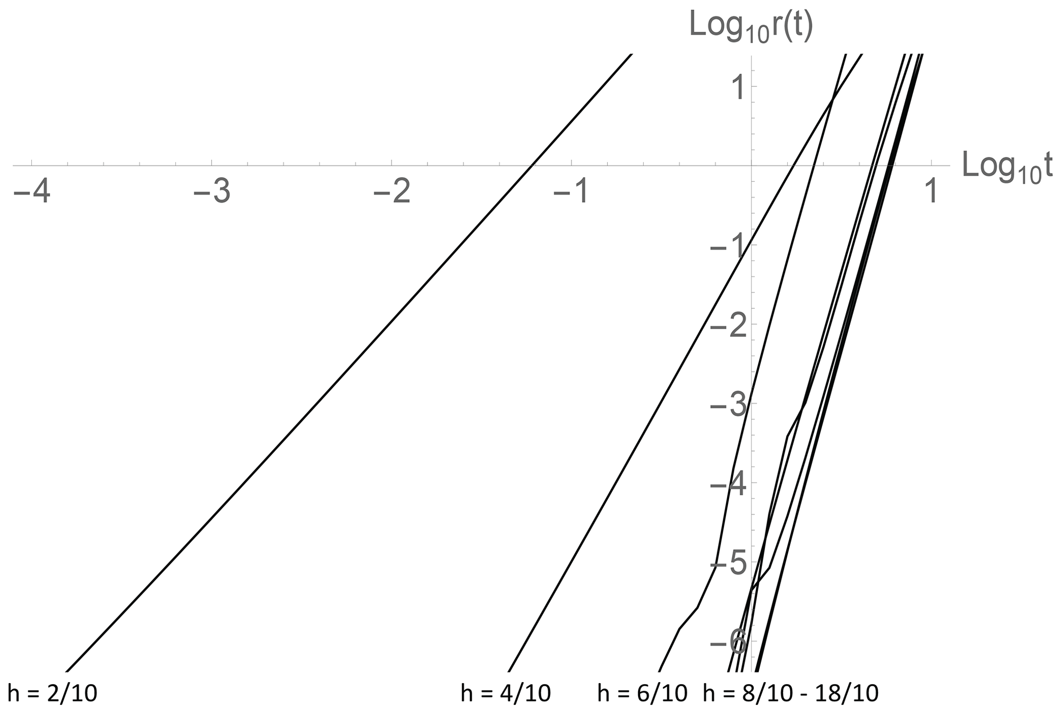
Figure A1This shows the logarithm of the relative error in the approximation (i.e. with 10 fractional terms and 10 integer-ordered terms) with respect to the deviation from the fGn R0,h(t) . The lines are for , , …, , (excluding the exponential case h=1), from left to right (note that convergence is only for irrational h, and therefore an extra 10−4 was added to each h). For the low h values the convergence is particularly slow.
A4 A convenient approximation
The expansion for Rα,h is the sum of a fractional-ordered and an integer-ordered series. Partial sums appear to converge (Fig. A1), albeit slowly. For simplicity, we consider the case of primary interest, a pure fRn process (α=0). Examination of partial sums shows that the integer-ordered and fractional-ordered terms tend to cancel, the difficulty being due to the coefficient of the integer-ordered terms that comes from the exponential integral and that can be large when . This suggests an alternative way of expressing the series:
where Dn is given by Eq. (A5) and the n sums start at n=2 since D1=0. Cj can be expressed as
where Φ is the Hurwitz–Lerch phi function .
We can also expand the exponential integral:
For the jmax and nmax partial sums, we have
Now define the (jmax, nmax) approximation by
This has the effect of adding half the next-highest n term and is more accurate; overall, jmax and nmax may now be taken to be much smaller than in the previous approximation. For example, putting nmax=2, jmax=1, we get with the partial sum
where
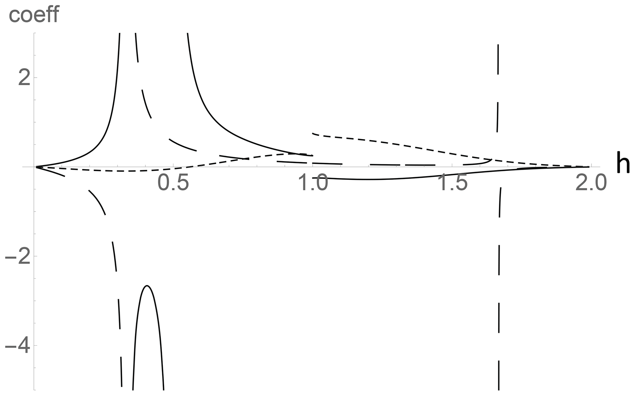
Figure A2The solid line is the constant term F1, the long dashes are the coefficients of the fractional power, and the short dashes are the coefficients of the linear term: . We can see that the contribution of the linear term (used in the approximation) for h<1 and t<1 is fairly small, whereas for , it is larger and the approximation is significantly better than the approximation (see Fig. A3).
To understand the behaviour, Fig. A2 shows the behaviour of the coefficient of the term , the constant term F1 and the coefficient of the next integer (linear in t) term
Up until the end of the fGn region (), the and F1 terms have opposite signs and tend to cancel. In addition, we see that for and h<1, they dominate over the (omitted) linear term. Figure A3 shows that the approximation is surprisingly good for h<1 and is still not so bad for . This approximation is thus useful for monthly-resolution macroweather temperature fields that have relaxation times of years or longer and where h is mostly over the range but over some tropical ocean regions can increase to as much as h≈1.2 (Del Rio Amador and Lovejoy, 2021a). Figure A3 shows that the (2,1) approximation is reasonably accurate for , especially for h<1.
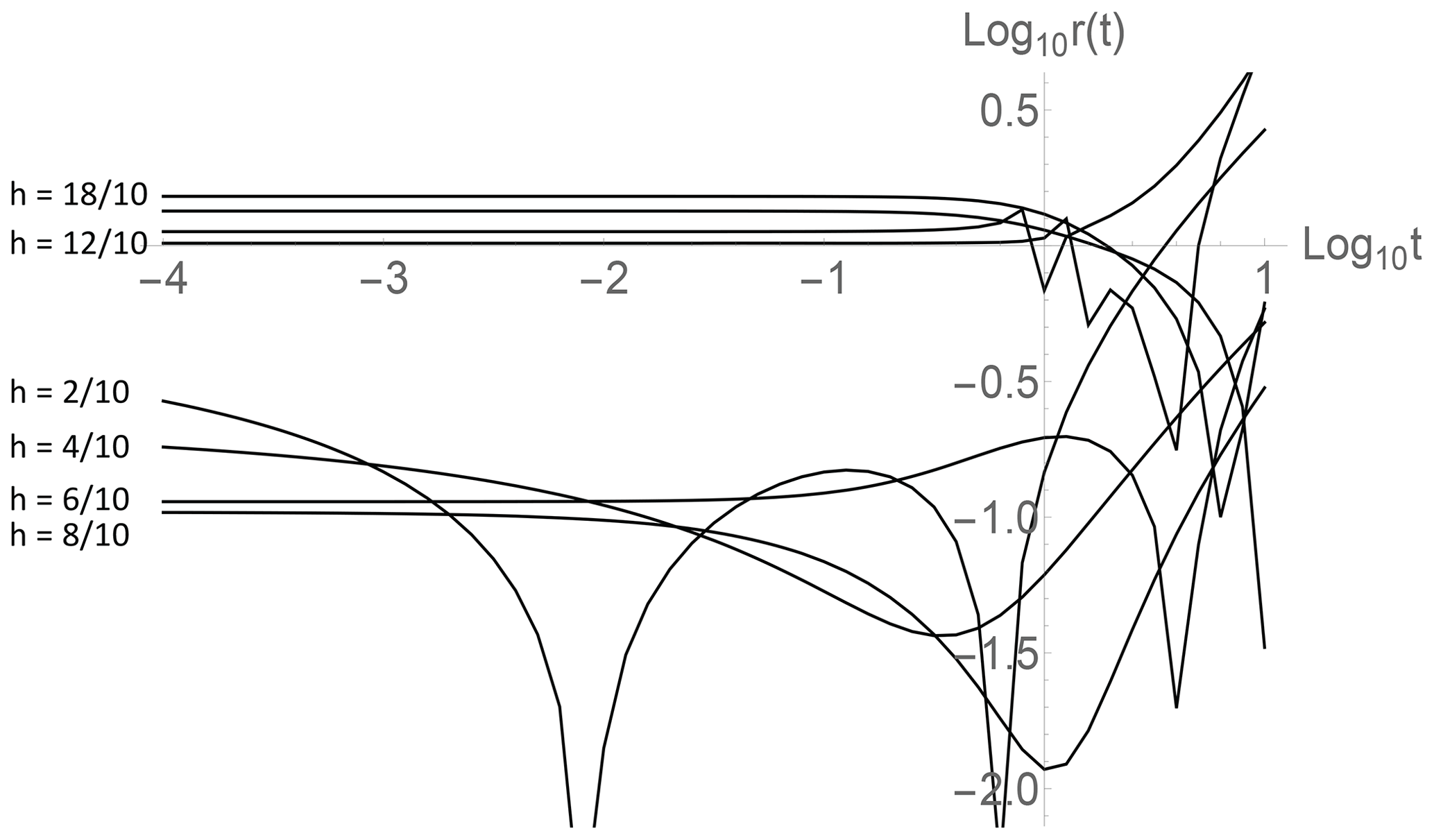
Figure A3This shows the logarithm of the relative error in the (2,1) approximation with respect to the deviation from the fGn Rh(t) (). For h<1, t<0 is of the order ≈30 %, whereas for h>1, it of the order 100 %. The h=1 (exponential) curve is not shown, although when t<0, the error is of order 60 %.
When α=0, , and the high-frequency fGn limit is an exact “ noise” (spectrum ω−1); it has both high- and low-frequency divergences. The high-frequency divergence can be tamed by averaging, but not the low-frequency divergence, so that fGn is only defined for . However, for fRn, the low frequencies are convergent over the whole range , and for we find that the correlation function has a logarithmic dependence at both small and large scales. This is associated with particularly slow transitions from high- to low-frequency behaviours. The critical value corresponds to the HEBE (Lovejoy, 2021a, b), where it was shown that the value could be derived analytically from the classical Budyko–Sellers energy balance equation. Therefore, and characterize the statistics of the temperature response of the classical heat equation response to an fGn-order α forcing.
It is possible to obtain exact analytic expressions for , and the Haar fluctuations; we develop these in this Appendix; for some early results, see Mainardi and Pironi (1996).
The starting point is the Laplace expression (Eq. A2) with :
We require the following Laplace transforms:
where we have introduced the incomplete gamma function: (with a branch cut in the complex plane from −∞ to 0). The general result is thus
Figure B1 shows plots over 8 orders of magnitude in t, indicating the generally very slow convergence to the asymptotic behaviour (shown as straight lines on the right).
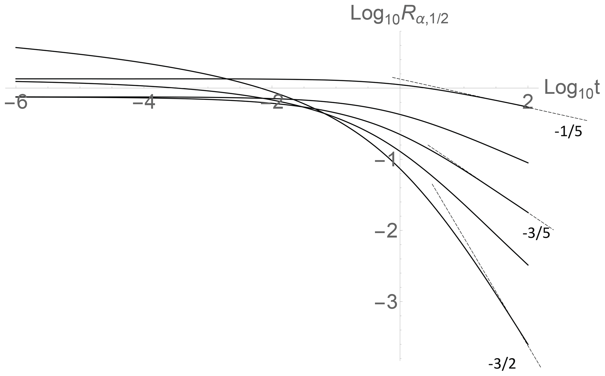
Figure B1 for α increasing from 0 (pure fRn) to in steps of (on the right: bottom to top). The α=0 curve has a logarithmic divergence at small t (far left). Recall from the section that at large t, and that for α>0, ; for α=0, , and the theoretical asymptotes of the leading terms are indicated for reference.
Figure B1 also shows the singular small t behaviour of the pure fRn case (α=0). In this limit both L1 and L2 are singular – they both yield logarithmic small-scale divergences. Pure fRn is of special interest and yields the somewhat simpler result:
We can use these results to obtain small and large t expansions:
where γE is Euler's constant=0.57… (the asymptotic formula can be obtained as a special case of Eq. A8 in Appendix A, but not the logarithmic small-scale divergence).
To obtain the corresponding results for , use
The exact is
where is the MeijrG function, Chi is the CoshIntegral function and Shi is the SinhIntegral function. The expansions are
We can also work out the variance of the Haar fluctuations:
Figure B2 shows numerical results for α=0 and . The transition between small and large t behaviour is extremely slow; the nine orders of magnitude depicted in the figure are barely enough. The extreme low ( (dashed) asymptotes on the left to a 0 slope (a square root logarithmic limit, Eq. B8) and to a slope on the right. The rms Haar fluctuation (black) changes slope from H=0 to (left to right). Figure B2 also shows the logarithmic derivative of the rms Haar (black) compared to a regression estimate over 2 orders of magnitude in scale (dashed; a factor of 10 smaller and 10 larger than the indicated scale was used; this represents a possibly empirically accessible range). This figure underlines the gradualness of the transition from H=0 to . If empirical data were available only over a factor of 100 in scale, depending on where this scale was with respect to the relaxation timescale (unity in the plot), the rms Haar fluctuations could have any slope in the range 0 to , with only small deviations.
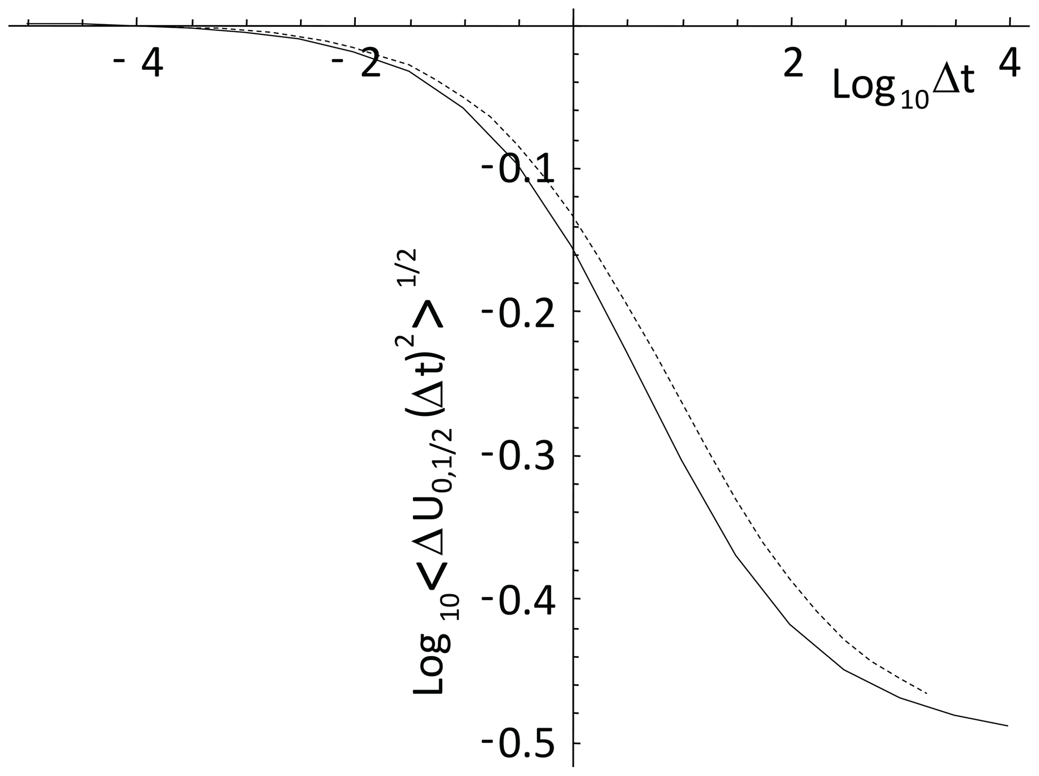
Figure B2The logarithmic derivative of the rms Haar fluctuations of (solid) in Fig. B1 compared to a regression estimate over 2 orders of magnitude in scale (dashed; factors of 10 smaller and 10 larger than the indicated scale were used). This plot underlines the gradualness of the transition from slopes 0 to −0.5 corresponding to apparent H=0 to scaling. Over a range of 100 or so in scale there is approximate scaling but with exponents that depend on the range of scales covered by the data. If data were available only over a factor of 100 in scale, the rms Haar fluctuations could have any slope in the fGn range 0 to , with only small deviations.
Mathematica code for generating sample fRn and fRm processes is available on request to the author. Analysis and simulation software is available from http://www.physics.mcgill.ca/~gang/software/doc/mathematicasoftware.17.9.14.nb.zip (last access: 14 February 2022; Lovejoy, 2014).
No data sets were used in this article.
The author is a member of the editorial board of Nonlinear Processes in Geophysics. The peer-review process was guided by an independent editor, and the author also has no other competing interests to declare.
Publisher's note: Copernicus Publications remains neutral with regard to jurisdictional claims in published maps and institutional affiliations.
This article is part of the special issue “Centennial issue on nonlinear geophysics: accomplishments of the past, challenges of the future”. It is not associated with a conference.
I thank Lenin Del Rio Amador, Roman Procyk, Raphaël Hébert, Cécile Penland, and Nicholas Watkins for discussions. We are also grateful for an exchange with Kristoffer Rypdal. We thank anonymous referees for suggestions, including the fifth referee for encouraging comments on the Fourier approach. This work was unfunded, and there were no conflicts of interest.
This paper was edited by Daniel Schertzer and reviewed by five anonymous referees.
Atanackovic, M., Pilipovic, S., Stankovic, B., and Zorica, D.: Fractional Calculus with applications in mechanics: variations and diffusion processes, Wiley, 313 pp., 2014.
Babenko, Y. I.: Heat and Mass Transfer, Khimiya, Leningrad, 1986 (in Russian).
Bender, C. M. and Orszag, S. A.: Advanced mathematical methods for scientists and engineers, Mc Graw Hill, 1978.
Biagini, F., Hu, Y., Øksendal, B., and Zhang, T.: Stochastic Calculus for Fractional Brownian Motion and Applications, Springer-Verlag, https://doi.org/10.1007/978-1-84628-797-8, 2008.
Budyko, M. I.: The effect of solar radiation variations on the climate of the earth, Tellus, 21, 611–619, 1969.
Buizza, R., Miller, M., and Palmer, T. N.: Stochastic representation of model uncertainties in the ECMWF Ensemble Prediction System, Q. J. Roy. Meteor. Soc., 125, 2887–2908, 1999.
Chekroun, M. D., Simonnet, E., and Ghil, M.: Stochastic Climate Dynamics: Random Attractors and Time-dependent Invariant Measures, Physica D, 240, 1685–1700, 2010.
Coffey, W. T., Kalmykov, Y. P., and Titov, S. V.: Characteristic times of anomalous diffusion in a potential, in: Fractional Dynamics: Recent Advances, edited by: Klafter, J., Lim, S., and Metzler, R., World Scientific, 51–76, 2012.
Del Rio Amador, L. and Lovejoy, S.: Predicting the global temperature with the Stochastic Seasonal to Interannual Prediction System (StocSIPS), Clim. Dynam., 53, 4373–4411, https://doi.org/10.1007/s00382-019-04791-4, 2019.
Del Rio Amador, L. and Lovejoy, S.: Using regional scaling for temperature forecasts with the Stochastic Seasonal to Interannual Prediction System (StocSIPS), Clim. Dynam., 57, 727–756, https://doi.org/10.1007/s00382-021-05737-5, 2021a.
Del Rio Amador, L. and Lovejoy, S.: Long-range Forecasting as a Past Value Problem: Untangling Correlations and Causality with scaling, Geophys. Res. Lett., 48, e2020GL092147, 2021b.
Dijkstra, H.: Nonlinear Climate Dynamics, Cambridge University Press, 357 pp., https://doi.org/10.1017/CBO9781139034135, 2013.
Franzke, C. and O'Kane, T. (Eds.): Nonlinear and Stochastic Climate Dynamics, Cambridge University Press, Cambridge, https://doi.org/10.1017/9781316339251, 2017.
Gripenberg, G. and Norros, I.: On the Prediction of Fractional Brownian Motion, J. Appl. Probab., 33, 400–410, 1996.
Hasselmann, K.: Stochastic Climate models, part I: Theory, Tellus, 28, 473–485, 1976.
Hébert, R.: A Scaling Model for the Forced Climate Variability in the Anthropocene, MSc thesis, McGill University, Montreal, 2017.
Hébert, R. and Lovejoy, S.: The runaway Green's function effect: Interactive comment on “Global warming projections derived from an observation-based minimal model” by K. Rypdal, Earth System Dyn. Disc., 6, C944–C953, 2015.
Hébert, R., Lovejoy, S., and Tremblay, B.: An Observation-based Scaling Model for Climate Sensitivity Estimates and Global Projections to 2100, Clim. Dynam., 56, 1105–1129 https://doi.org/10.1007/s00382-020-05521-x, 2021.
Herrmann, R.: Fractional Calculus: an Introduction for Physicists, World Scientific, ISBN: 139789814340243, 2011.
Hilfer, R. (Ed.): Applications of Fractional Calculus in Physics, World Scientific, ISBN: 9810234570, 2000.
Hipel, K. W. and McLeod, A. I.: Time series modelling of water resources and environmental systems, 1st edn., Elsevier, ISBN: 9780080870366, 1994.
IPCC: Climate Change 2013: The Physical Science Basis. Contribution of Working Group I to the Fifth Assessment Report of the Intergovernmental Panel on Climate Change, Cambridge University Press, Cambridge, ISBN: 9781107661820, 2013.
Jumarie, G.: Stochastic differential equations with fractional Brownian motion inputs, Int. J. Syst. Sci., 24, 1113–1131, 1993.
Karczewska, A. and Lizama, C.: Solutions to stochastic fractional relaxation equations, Phys. Scripta, T136, 7 pp., https://doi.org/10.1088/0031-8949/2009/T136/014030, 2009.
Kou, S. C. and Sunney Xie, X.: Generalized Langevin Equation with Fractional Gaussian Noise: Subdiffusion within a Single Protein Molecule, Phys. Rev. Lett., 93, 4, https://doi.org/10.1103/PhysRevLett.93.180603, 2004.
Lovejoy, S.: What is climate?, EOS, 94, 1–2, 2013.
Lovejoy, S.: Mathematica software for simulation and analysis of scaling and multifractals, Department of Physics, McGill University, http://www.physics.mcgill.ca/~gang/software/doc/mathematicasoftware.17.9.14.nb.zip (last access: 14 February 2022), 2014.
Lovejoy, S.: A voyage through scales, a missing quadrillion and why the climate is not what you expect, Clim. Dynam., 44, 3187–3210, https://doi.org/10.1007/s00382-014-2324-0, 2015a.
Lovejoy, S.: Using scaling for macroweather forecasting including the pause, Geophys. Res. Lett., 42, 7148–7155, https://doi.org/10.1002/2015GL065665, 2015b.
Lovejoy, S.: The spectra, intermittency and extremes of weather, macroweather and climate, Nature Scientific Reports, 8, 1–13, https://doi.org/10.1038/s41598-018-30829-4, 2018.
Lovejoy, S.: Weather, Macroweather and Climate: our random yet predictable atmosphere, Oxford University Press, 334 pp., ISBN: 978-0-19-086421-7, 2019.
Lovejoy, S.: The half-order energy balance equation – Part 1: The homogeneous HEBE and long memories, Earth Syst. Dynam., 12, 469–487, https://doi.org/10.5194/esd-12-469-2021, 2021a.
Lovejoy, S.: The half-order energy balance equation – Part 2: The inhomogeneous HEBE and 2D energy balance models, Earth Syst. Dynam., 12, 489–511, https://doi.org/10.5194/esd-12-489-2021, 2021b.
Lovejoy, S. and Schertzer, D.: The Weather and Climate: Emergent Laws and Multifractal Cascades, Cambridge University Press, 496 pp., ISBN: 978-1-107-01898-3, 2013.
Lovejoy, S., Del Rio Amador, L., and Hébert, R.: Harnessing butterflies: theory and practice of the Stochastic Seasonal to Interannual Prediction System (StocSIPS), in: Nonlinear Advances in Geosciences, edited by: Tsonis, A. A., Springer Nature, 305–355, https://doi.org/10.1007/978-3-319-58895-7_17, 2017.
Lovejoy, S., del Rio Amador, L., and Hébert, R.: The ScaLIng Macroweather Model (SLIMM): using scaling to forecast global-scale macroweather from months to decades, Earth Syst. Dynam., 6, 637–658, https://doi.org/10.5194/esd-6-637-2015, 2015.
Lovejoy, S., Procyk, R., Hébert, R., and del Rio Amador, L.: The Fractional Energy Balance Equation, Q. J. Roy. Meteor. Soc., 1–25, https://doi.org/10.1002/qj.4005, 2021.
Lutz, E.: Fractional Langevin equation, Phys. Rev. E, 64, 4, https://doi.org/10.1103/PhysRevE.64.051106, 2001.
Magin, R., Sagher, Y., and Boregowda, S.: Application of fractional calculus in modeling and solving the bioheat equation, in: Design and Nature II, edited by: Collins, M. W. and Brebbia, C. A., WIT Press, 207–216, ISBN: 1-85312-721-3, 2004.
Mainardi, F. and Pironi, P.: The Fractional Langevin Equation: Brownian Motion Revisited, Extracta Mathematicae, 10, 140–154, 1996.
Mandelbrot, B. B.: The Fractal Geometry of Nature, Freeman, ISBN-10.0716711869, 1982.
Mandelbrot, B. B. and Van Ness, J. W.: Fractional Brownian motions, fractional noises and applications, SIAM Rev., 10, 422–450, 1968.
Mandelbrot, B. B. and Wallis, J. R.: Computer Experiments with fractional gaussian noises: part 3, mathematical appendix, Water Resour. Res., 5, 260–267, https://doi.org/10.1029/WR005i001p00260, 1969.
Mathews, J. and Walker, R. L.: Mathematical methods of Physics, W. A. Benjamin, ISBN: 8053-7002-1, 1973.
Metzler, R. and Klafter, J.: The Random Walks Guide To Anomalous Diffusion: A Fractional Dynamics Approach, Phys. Rep., 339, 1–77, 2000.
Newman, M.: An Empirical Benchmark for Decadal Forecasts of Global Surface Temperature Anomalies, J. Climate, 26, 5260–5269, https://doi.org/10.1175/JCLI-D-12-00590.1, 2013.
Nonnenmacher, T. F. and Metzler, R.: Applications of fractional calculus techniques to problems in biophysics, in: Fractional Calculus in Physics, edited by: Hilfer, R., World Scientific, 377–427, ISBN: 9810234570, 2000.
North, G. R. and Kim, K. Y.: Energy Balance Climate Models, Wiley-VCH, 369 pp., ISBN: 978-3-527-41132-0, 2017.
Oldham, K. B.: Diffusive transport to planar, cylindrical and spherical electrodes, J. Electroanal. Chem. Interfacial Electrochem., 41, 351–358, 1973.
Oldham, K. B. and Spanier, J.: A general solution of the diffusion equation for semi infinite geometries, J. Math. Anal. Appl., 39, 665–669, 1972.
Palma, W.: Long-memory time series, Wiley, ISBN: 9780470114025, 2007.
Palmer, T. N. and Williams, P. (Eds.): Stochastic physics and Climate models, Cambridge University Press, Cambridge, 480 pp., ISBN: 9780521761055, 2010.
Papoulis, A.: Probability, Random Variables and Stochastic Processes, Mc Graw Hill, ISBN-10: 0070484481, 1965.
Penland, C.: A stochastic model of IndoPacific sea surface temperature anomalies, Phys. D, 98, 534–558, 1996.
Penland, C. and Magorian, T.: Prediction of Nino 3 sea surface temperatures using linear inverse modeling, J. Climate, 6, 1067–1076, 1993.
Podlubny, I.: Fractional Differential Equations, Academic Press, 340 pp., ISBN 9780125588409, 1999.
Procyk, R.: The Fractional Energy Balance Equation: the Unification of Externally Forced and Internal Variability, MSc thesis, McGill University, Montreal, Canada, 111 pp., 2021.
Procyk, R., Lovejoy, S., and Hébert, R.: The fractional energy balance equation for climate projections through 2100, Earth Syst. Dynam., 13, 81–107, https://doi.org/10.5194/esd-13-81-2022, 2020.
Procyk, R., Lovejoy, S., and Hébert, R.: The fractional energy balance equation for climate projections through 2100, Earth Syst. Dynam., 13, 81–107, https://doi.org/10.5194/esd-13-81-2022, 2022.
Rypdal, K.: Global temperature response to radiative forcing: Solar cycle versus volcanic eruptions, J. Geophys. Res., 117, D06115, https://doi.org/10.1029/2011JD017283, 2012.
Rypdal, K.: Global warming projections derived from an observation-based minimal model, Earth Syst. Dynam., 7, 51–70, https://doi.org/10.5194/esd-7-51-2016, 2016.
Sardeshmukh, P., Compo, G. P., and Penland, C.: Changes in probability assoicated with El Nino, J. Climate, 13, 4268–4286, 2000.
Sardeshmukh, P. D. and Sura, P.: Reconciling non-gaussian climate statistics with linear dynamics, J. Climate, 22, 1193–1207, 2009.
Schertzer, D., Larchevíque, M., Duan, J., Yanovsky, V. V., and Lovejoy, S.: Fractional Fokker-Planck equation for nonlinear stochastic differential equation driven by non-Gaussian Levy stable noises, J. Math. Phys., 42, 200–212, 2001.
Schiessel, H., Friedrich, C., and Blumen, A.: Applications to problems in polymer physics and rheology, in: Fractional Calculus in physics, edited by: Hilfer, R., World Scientific, 331–376, ISBN: 9810234570, 2000.
Sellers, W. D.: A global climate model based on the energy balance of the earth-atmosphere system, J. Appl. Meteorol., 8, 392–400, 1969.
Sierociuk, D., Dzielinski, A., Sarwas, G., Petras, I., Podlubny, I., and Skovranek, T.: Modelling heat transfer in heterogeneous media using fractional calculus, Philos. T. R. Soc. A, 371, 20120146, https://doi.org/10.1098/rsta.2012.0146, 2013.
van Hateren, J. H.: A fractal climate response function can simulate global average temperature trends of the modern era and the past millennium, Clim. Dynam., 40, 2651, https://doi.org/10.1007/s00382-012-1375-3, 2013.
Vojta, T., Skinner, S., and Metzler, R.: Probability density of the fractional Langevin equation with reflecting walls, Phys. Rev. E, 100, 042142, https://doi.org/10.1103/PhysRevE.100.042142, 2019.
Watkins, N.: Fractional Stochastic Models for Heavy Tailed, and Long-Range Dependent, Fluctuations in Physical Systems, in: Nonlinear and Stochastic Climate Dynamics, edited by: Franzke, C. and O'Kane, T., Cambridge University Press, 340–368, ISBN: 9781316339251, 2017.
Watkins, N., Chapman, S., Klages, R., Chechkin, A., Ford, I., and Stainforth, D.: Generalised Langevin Equations and the Climate Response Problem, Earth and Space Science Open Archive, https://doi.org/10.1002/essoar.10501367.1, 2019.
Watkins, N. W., Chapman, S. C., Chechkin, A., Ford, I., Klages, R., and Stainforth, D. A.: On Generalized Langevin Dynamics and the Modelling of Global Mean Temperature, arXiv [preprint], arXiv:2007.06464v1, 4 December 2020.
West, B. J., Bologna, M., and Grigolini, P.: Physics of Fractal Operators, Springer, 354 pp., ISBN: 0-387-95554-2, 2003.
Ziegler, E. and Rehfeld, K.: TransEBM v. 1.0: description, tuning, and validation of a transient model of the Earth's energy balance in two dimensions, Geosci. Model Dev., 14, 2843–2866, https://doi.org/10.5194/gmd-14-2843-2021, 2021.
- Abstract
- Introduction
- The fractional relaxation equation
- Application to fBm, fGn, fRm, and fRn
- Prediction
- Conclusions
- Appendix A: The small- and large-scale fRn and fRm statistics
- Appendix B: The special case
- Code availability
- Data availability
- Competing interests
- Disclaimer
- Special issue statement
- Acknowledgements
- Review statement
- References